UT-14-23

Construction of Gaiotto states with fundamental multiplets
through Degenerate DAHA
Yutaka Matsuo^∗, Chaiho Rim^† and Hong Zhang^†
∗ Department of Physics, The University of Tokyo, Bunkyo-ku, Tokyo, Japan

^† Department of Physics and Center for Quantum Spacetime (CQUeST)
Sogang University, Seoul 121-742, Korea

We construct Gaiotto states with fundamental multiplets in $SU(N)$ gauge theories, in terms of the orthonormal basis of spherical degenerate double affine Hecke algebra (SH in short), the representations of which are equivalent to those of $W_{n}$ algebra with additional $U(1)$ current. The generalized Whittaker conditions are demonstrated under the action of SH, and further rewritten in terms of $W_{n}$ algebra. Our approach not only consists with the existing literature but also holds for general $SU(N)$ case.

1 Introduction

The instanton Nekrasov partition function[1, 2, 3] for 4 dimensional ${\cal N}=2$ supersymmetric $SU(2)$ quiver gauge theory has the remarkable correspondence with 2 dimensional Liouville conformal field theories, so called AGT conjecture [4]. And the correspondence was generalized into $SU(N)$ quiver gauge theories in [5, 6] .

There are various proofs for the AGT conjecture [7, 8, 9, 10, 11]. In most cases, the Virasoro and W algebras play the essential role. In contrast, spherical degenerate double affine Hecke algebra (spherical DDAHA or SH) [12, 13, 14, 15, 16] turns out to be another useful tool to prove the AGT conjecture. DDAHA is generated by $2N$ operators, $z_{i}$ and $\mathcal{D}_{i}$ ($i=1,\cdots,N$) where

$$\mathcal{D}_{i}=z_{i}\nabla_{i}+\sum_{j<i}\sigma_{ij},\quad\nabla_{i}=\frac{\partial}{\partial z_{i}}+\beta\sum_{j(\neq i)}\frac{1}{z_{i}-z_{j}}(1-\sigma_{ij})\,.$$ (1)

and permutation operators. Here $\nabla_{i}$ is the Dunkl operator which plays a fundamental role in Calogero-Sutherland system and $\sigma_{ij}$ is the transposition of variables, $z_{i}\sigma_{ij}=\sigma_{ij}z_{j}$. The operators $z_{i}$ and $\mathcal{D}_{i}$ satisfies the following commutation relations,

$$[z_{i},z_{j}]=0,\qquad[\mathcal{D}_{i},\mathcal{D}_{j}]=0\,,$$ (2)

$$[\mathcal{D}_{i},z_{j}]=\left\{\begin{array}[]{ll}-\beta z_{i}\sigma_{ij}&i<j\\ z_{i}+\beta\Big{(}\sum_{k<i}z_{k}\sigma_{ik}+\sum_{k>i}z_{i}\sigma_{ik}\Big{)}&i=j\\ -\beta z_{j}\sigma_{ij}&i>j\,.\end{array}\right.$$ (6)

DDAHA is the algebra freely generated by $z_{i},D_{i}$ and $\sigma\in S_{N}$. Spherical DDAHA (SH) is obtained by the restriction to the symmetric part. For the special value of $\beta=1$, SH reduces to $\mathcal{W}_{1+\infty}$ algebra which is described by free fermions.

Recently it was found that some representations of SH are equivalent to those of $W_{n}$ algebra with additional $U(1)$ current [15]. It is known that SH has a natural action on the equivariant cohomology class of the instanton moduli space while $W_{n}$ algebra describes the symmetry of Toda field theory. This correspondence was used to prove the AGT conjecture. For example, in [15] such mechanism was applied to the pure $SU(N)$ super Yang-Mills theory, and the representative of the cohomology class is mapped to the orthogonal basis in the Hilbert space of $W_{n}$ algebra. In this way, the Gaiotto state [17] is constructed to arbitrary order through the conditions on the action of the generators of SH. Later in [16], such correspondence was applied to quiver type gauge theories. The action of SH on the basis appears as the recursion relation for the Nekrasov partition function, which is then interpreted as the Ward identities associated with the $W_{n}$-algebra.

Here we apply the similar trick to construct explicit Gaiotto states with fundamental multiplets in $SU(N)$ gauge theories. The computation is in parallel with those in [15]. Note that the Gaiotto state appears as an irregular module of Virasoro and $W_{n}$ algebra. There were already a few attempts to construct the irregular states algebraically in [17, 18, 19]. Our construction is not limited to $SU(3)$ but is extended to $SU(N)$ with $N_{f}<N$.

It is also noted that the Gaiotto state construction was proposed but in a different manner, which uses the coherent state approach in [20, 21]. Some of irregular state was constructed explicitly using random matrix formalism in connection with $SU(2)$ quiver gauge theories [22]. Thus, our construction will be instructive and complementary to understand the Gaiotto state in different approaches.

This paper is organizes as follows. In section 2 we define the Gaiotto states with fundamental multiplets in terms of the orthonormal basis of SH. In section 3, we briefly review the algebra SH and the relation with $W_{n}$ algebra. In section 4, we give the explicit correspondence between SH and $W_{n}$ generators through the use of free boson fields. In section 5 we show that the states satisfy generalized Whittaker condition in terms of SH. Finally in section 6 we rewrite the conditions in terms of the generators of $W_{n}$ algebra and confirm the consistency with the existing literature [18, 19, 20].

In the appendix, we derive the Ward identities for the Virasoro operator $L_{\pm 2}$. Though this is not directly relevant to the main claim of this paper, we include it since the analysis is technically very close and also it completes the analysis of [16].

2 Construction of Gaiotto States

For the pure super Yang-Mills theory where the fundamental multiplet is absent, $N_{f}=0$, the instanton part of the partition function has the form,

$$Z(\vec{a})=\sum_{\vec{Y}}\Lambda^{4|\vec{Y}|}Z_{\text{vect}}(\vec{a},\vec{Y}),$$ (7)

with

$$Z_{\text{vect}}(\vec{a},\vec{Y}):=f(\vec{a},\vec{Y}):=\prod_{p,q}\frac{1}{g_{Y_{p}Y_{q}}(a_{p}-a_{q})}$$ (8)

where $\Lambda$ is the dynamical scale, $\vec{a}\in\mathbf{C}^{n}$ is the VEV for an adjoint scalar field in the vector multiplet and $\vec{Y}=(Y_{1},\cdots,Y_{N})$ is a set of Young tableaux characterizing fixed points of localization in the instanton moduli space. And

$$g_{Y,W}(x) = \prod_{(i,j)\in Y}(x+\beta(Y^{\prime}_{j}-i+1)+W_{i}-j)\prod_{(i,j)\in W}(-x+\beta(W^{\prime}_{j}-i)+Y_{i}-j+1)\,,$$ (9)

where $Y_{i}$ is the $i$th column of $Y$, and $Y^{\prime}$ stands for the transposed Young tableaux. $\beta$ is related to $\Omega$-deformation parameters by $\beta=-\epsilon_{1}/\epsilon_{2}$.

According to AGT conjecture, we may put the partition function as the inner product of two Gaiotto states $Z(\vec{a})=\langle\tilde{G}|G\rangle$. It is a nontrivial issue to realize $|G\rangle$ in the Hilbert space of W-algebra. On the other hand, in SH, we know the orthonormal basis and the action of generators which will be reviewed in the next section. The Gaiotto state takes the form,

$$|G\rangle = \sum_{\vec{Y}}\Lambda^{2|\vec{Y}|}(Z_{\text{vect}}(\vec{a},\vec{Y}))^{1/2}|\vec{a},\vec{Y}\rangle\,.$$ (10)

Here $|\vec{a},\vec{Y}\rangle$ is introduced in [16] as an basis of a Hilbert space $\mathcal{H}_{\vec{a}}$. The dual basis $\langle\vec{a},\vec{Y}|$ is defined such that $\langle\vec{a},\vec{Y}|\vec{a},\vec{W}\rangle=\delta_{\vec{Y},\vec{W}}\,.$ It is trivial to confirm that it has the desired inner product due to the orthonormal property of the basis. However, it is nontrivial to confirm that it satisfies the condition for generalized Whittaker condition as given in [15].

One may proceed likewise for $N_{f}=2$. The partition function has extra contributions from the fundamental multiplets with masses $m_{i}$,

$$Z^{N_{f}=2}(\vec{a},m_{1},m_{2},\Lambda)=\sum_{\vec{Y}}\Lambda^{2|\vec{Y}|}Z_{\text{vect}}(\vec{a},\vec{Y})Z_{\text{fund}}(\vec{a},\vec{Y},m_{1})Z_{\text{fund}}(\vec{a},\vec{Y},m_{2})$$ (11)

where

$$Z_{\text{fund}}(\vec{a},\vec{Y},m)=\prod_{p=1}^{N}\prod_{(i,j)\in Y_{p}}(a_{p}+\beta i-j-m)$$ (12)

Noting that

$$Z^{N_{f}=2}(\vec{a},m_{1},m_{2},\Lambda)=\langle G,m_{2}|G,m_{1}\rangle$$ (13)

one may have the Gaiotto state with one additional parameter $m$

$$|G,m\rangle = \sum_{\vec{Y}}\Lambda^{|\vec{Y}|}(Z_{\text{vect}}(\vec{a},\vec{Y}))^{1/2}Z_{\text{fund}}(\vec{a},\vec{Y},m)\,|\vec{a},\vec{Y}\rangle\,.$$ (14)

In this way, it is straightforward to generalize it to additional $k<N$ parameters $m_{1},m_{2},\cdots,m_{k}$, namely,

$$|G,m_{1},\cdots,m_{k}\rangle = \sum_{\vec{Y}}\Lambda^{|\vec{Y}|}(Z_{\text{vect}}(\vec{a},\vec{Y}))^{1/2}\prod_{A=1}^{k}(Z_{\text{fund}}(\vec{a},\vec{Y},m_{A}))|\vec{a},\vec{Y}\rangle\,.$$ (15)

One may easily confirm that the inner product of two Gaiotto states with $k$ parameters will give the instanton partition function with $N_{f}=2k$. The nontrivial part is to confirm the Whittaker vector conditions. The case for $N_{f}=0$ was given by [15]. The proof for additional fundamental multiplets is new. Our task is to find the generalized Whittaker conditions using SH generators and rewrite them in terms of $W_{n}$ generators.

3 Brief introduction of SH

The generators of Spherical DDAHA (SH) are obtained by symmetrizing those of DDAHA by $\mathcal{S}=\frac{1}{N!}\sum_{\sigma\in S_{N}}\sigma$, $\mathcal{S}\mathcal{O}\mathcal{S}$ where $\mathcal{O}\in\mbox{DDAHA}$. Such generators act naturally on the ring of symmetric functions of $z_{i}$. The independent generators of SH is given by $D_{nm}\sim\mathcal{S}\sum_{i=1}^{N}(z_{i})^{n}(\mathcal{D}_{i})^{m}\mathcal{S}$ ($n\in\mathbf{Z}$, $m\in\mathbf{Z}_{\geq 0}$) in $N\rightarrow\infty$ limit. The definition of $D_{nm}$ is only sketchy here and will be more carefully defined later. For a special value for $\beta=1$, SH reduces to $\mathcal{W}_{1+\infty}$ algebra which is described by free fermions.

In large $N$ limit, one may introduce free boson description of SH in terms of power sum polynomial $p_{n}=\sum_{i=1}^{\infty}(z_{i})^{n}$. We identify,

$$p_{n}:=\alpha_{-n},\quad n\frac{\partial}{\partial p_{n}}:=\alpha_{n},\quad n\in\mbox{Z}_{\geq 0}\,$$ (16)

which satisfies the standard commutation relation $[\alpha_{n},\alpha_{m}]=n\delta_{n+m,0}$. The space of symmetric functions is described by the Fock space ${\mathcal{F}}$ of the free boson.

The Hilbert of $W_{n}$-algebra shows up when we take coproduct of $n$ representations of ${\mathcal{F}}$ and make some restriction on the representation (taking the ‘symmetric part’ which is referred as $[1^{n}]$ representation in [15]). After taking such coproduct it has nontrivial central charges given below. To distinguish the algebra with central extensions from others, we will denote the algebra SH^c. It has generators $D_{r,s}$ with $r\in\mathbf{Z}$ and $s\in\mathbf{Z}_{\geq 0}$. The commutation relations for degree $\pm 1,0$ generators are defined by,

$$\left[D_{0,l},D_{1,k}\right] = D_{1,l+k-1},\;\;\;l\geq 1\,,$$ (17)

$$\left[D_{0,l},D_{-1,k}\right] = -D_{-1,l+k-1},\;\;\;l\geq 1\,,$$ (18)

$$\left[D_{-1,k},D_{1,l}\right] = E_{k+l}\;\;\;l,k\geq 0\,,$$ (19)

$$\left[D_{0,l},D_{0,k}\right] = 0\,,\,\,k,l\geq 0\,,$$ (20)

where $E_{k}$ is a nonlinear combination of $D_{0,k}$ determined in the form of a generating function,

$$1+(1-\beta)\sum_{l\geq 0}E_{l}s^{l+1}=\exp(\sum_{l\geq 0}(-1)^{l+1}c_{l}\pi_{l}(s))\exp(\sum_{l\geq 0}D_{0,l+1}\omega_{l}(s))\,,$$ (21)

with

$$\pi_{l}(s)=s^{l}G_{l}(1+(1-\beta)s)\,,$$ (22)

$$\omega_{l}(s)=\sum_{q=1,-\beta,\beta-1}s^{l}(G_{l}(1-qs)-G_{l}(1+qs))\,,$$ (23)

$$G_{0}(s)=-\log(s),\;\;\;G_{l}(s)=(s^{-l}-1)/l\;\;\;l\geq 1\,.$$ (24)

The parameters $c_{l}$ ($l\geq 0$) are central charges. Other generators are defined recursively by,

$$D_{l+1,0}=\frac{1}{l}\left[D_{1,1},D_{l,0}\right], D_{-l-1,0}=\frac{1}{l}\left[D_{-l,0},D_{-1,1}\right]\,,$$ (25)

$$D_{r,l}=\left[D_{0,l+1},D_{r,0}\right]\;\;\; D_{-r,l}=\left[D_{-r,0},D_{0,l+1}\right]\,.$$ (26)

for $l\geq 0,r>0$ .

There is an explicit form of the action on the orthonormal basis $|\vec{a},\vec{Y}\rangle$,

$$D_{-1,l}|\vec{a},\vec{Y}\rangle = (-1)^{l}\sum_{q=1}^{N}\sum_{t=1}^{{f_{q}}}(a_{q}+B_{t}(Y_{q}))^{l}\Lambda^{(t,-)}_{q}(\vec{Y})|\vec{a},\vec{Y}^{(t,-),q}\rangle\,,$$ (27)

$$D_{1,l}|\vec{a},\vec{Y}\rangle = (-1)^{l}\sum_{q=1}^{N}\sum_{t=1}^{{f_{q}}+1}(a_{q}+A_{t}(Y_{q}))^{l}\Lambda^{(t,+)}_{q}(\vec{Y})|\vec{a},\vec{Y}^{(t,+),q}\rangle\,,$$ (28)

$$D_{0,l+1}|\vec{a},\vec{Y}\rangle = (-1)^{l}\sum_{q=1}^{N}\sum_{\mu\in Y_{q}}(a_{q}+c(\mu))^{l}|\vec{a},\vec{Y}\rangle\,.$$ (29)

where $c(\mu)=\beta i-j\mbox{ for }\mu=(i,j).$

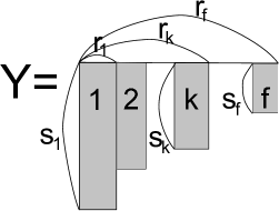
Figure 1: Decomposition of Young diagram by rectangles

The factor $\Lambda^{(t,-)}_{q}(\vec{a},\vec{Y})$ is defined by

$$\Lambda^{(k,+)}_{p}(\vec{a},\vec{Y}) = \left(\prod_{q=1}^{N}\left(\prod_{\ell=1}^{f_{q}}\frac{a_{p}-a_{q}+A_{k}(Y_{p})-B_{\ell}(Y_{q})+\xi}{a_{p}-a_{q}+A_{k}(Y_{p})-B_{\ell}(Y_{q})}{\prod}_{\ell=1}^{\prime f_{q}+1}\frac{a_{p}-a_{q}+A_{k}(Y_{p})-A_{\ell}(Y_{q})-\xi}{a_{p}-a_{q}+A_{k}(Y_{p})-A_{\ell}(Y_{q})}\right)\right)^{1/2}\,,$$ (30)

$$\Lambda^{(k,-)}_{p}(\vec{a},\vec{Y}) = \left(\prod_{q=1}^{N}\left(\prod_{\ell=1}^{f_{q}+1}\frac{a_{p}-a_{q}+B_{k}(Y_{p})-A_{\ell}(Y_{q})-\xi}{a_{p}-a_{q}+B_{k}(Y_{p})-A_{\ell}(Y_{q})}{\prod}_{\ell=1}^{\prime f_{q}}\frac{a_{p}-a_{q}+B_{k}(Y_{p})-B_{\ell}(Y_{q})+\xi}{a_{p}-a_{q}+B_{k}(Y_{p})-B_{\ell}(Y_{q})}\right)\right)^{1/2}\,.$$ (31)

We decompose $Y$ into rectangles $Y=(r_{1},\cdots,r_{f};s_{1},\cdots,s_{f})$ (with $0<r_{1}<\cdots<r_{f}$, $s_{1}>\cdots>s_{f}>0$, see Figure 1 for the parametrization). We use $f_{p}$ (resp. $\bar{f}_{p}$) to represent the number of rectangles of $Y_{p}$ (resp $W_{p}$). The factors $A_{k}(Y_{p})$, $B_{\ell}(Y_{q})$ are

$$A_{k}(Y) = \beta r_{k-1}-s_{k}-\xi,\quad(k=1,\cdots,f+1)\,,$$ (32)

$$B_{k}(Y) = \beta r_{k}-s_{k},\quad(k=1,\cdots,f)\,,$$ (33)

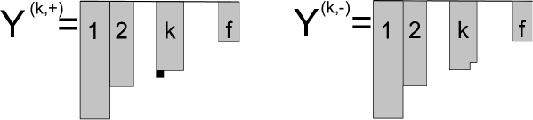
Figure 2: Locations of boxes

where $\xi:=1-\beta$. $A_{k}(Y)$ (resp. $B_{k}(Y)$) represents the $k^{\mathrm{th}}$ location where a box may be added to (resp. deleted from) the Young diagram $Y$ composed with a map from location to $\mathbf{C}$.

We denote $Y^{(k,+)}$ (resp. $Y^{(k,-)}$) as the Young diagram obtained from $Y$ by adding (resp. deleting) a box at $(r_{k-1}+1,s_{k}+1)$ (resp. $(r_{k},s_{k})$). Similarly we use the notation $\vec{Y}^{(k\pm),p}=(Y_{1},\cdots,Y_{p}^{(k,\pm)},\cdots,Y_{N})$ to represent the variation of one Young diagram in a set of Young tables $\vec{Y}$. For more detail of the notation, we refer [16].

4 The relation between SH^c and $W$-algebra

SH^c and $W_{n}$-algebra look very different but the Hilbert space of both algebras are identical for $[1^{n}]$ representation of SH^c. The content of this section is a brief summary of [15].

The generators of $W_{n}$-algebra are defined through the quantum Miura transformation,

$$-:\prod_{j=1}^{n}(Q\partial_{z}+\vec{h}_{j}\cdot\partial\vec{\varphi}):=\sum_{d=0}^{n}W^{(d)}(z)(Q\partial_{z})^{n-d}\,.$$ (34)

where $\vec{h}_{i}=\vec{e}_{i}-\frac{1}{n}\sum_{i=1}^{n}\vec{e}_{i}$ and $\vec{e}_{i}$ is the $i$-th orthonormal basis of $\mathbf{R}^{n}$. $\partial\vec{\varphi}=(\partial\varphi_{1},\cdots,\partial\varphi_{n})$ is $n$ free bosons with the standard OPE,

$$\partial\varphi_{i}(z)\partial\varphi_{j}(0)\sim\frac{\delta_{ij}}{z^{2}}\,,\quad\partial\varphi_{i}(z)=\sum_{r\in\mathbf{Z}}\alpha_{r}^{(i)}z^{-r-1}\,.$$ (35)

We introduce $\mathcal{J}(z)=\sum_{i=1}^{n}\partial\varphi_{i}(z)$ to describe the $U(1)$ factor.

Expansion of (34) gives,

$$W^{(0)}(z) = -1,$$ (36)

$$W^{(1)}(z) = 0,$$ (37)

$$W^{(2)}(z) = \frac{1}{2}(\partial\vec{\varphi})^{2}-\frac{1}{2n}:\mathcal{J}^{2}(z):+Q\vec{\rho}\cdot\partial^{2}\vec{\varphi},$$ (38)

with $\vec{\rho}=(-\frac{n-1}{2},-\frac{n-3}{2},\cdots,\frac{n-1}{2})$. $W^{(2)}$ is the standard form of Virasoro generators with the central charge, $c=(n-1)(1-Q^{2}n(n+1))$. The higher generators are in general complicated but the part with highest power of $\partial\varphi$ is written in a relatively simple way,

$$W^{(d)} = -\sum_{j_{1}<\cdots<j_{d}}:(\vec{h}_{j_{1}}\cdot\partial\vec{\varphi})\cdots(\vec{h}_{j_{d}}\cdot\partial\vec{\varphi}):+\mbox{ lower terms}$$ (41)

$$= -\sum_{s=0}^{d}(-n)^{s-d}\left(\begin{array}[]{c}n-s\\ n-d\end{array}\right)\sum_{j_{1}<\cdots<j_{s}}:\mathcal{J}(z)^{d-s}\partial\varphi_{j_{1}}(z)\cdots\partial\varphi_{j_{s}}(z)+\mbox{ lower terms}\,.$$

Meanwhile, SH^c is given in free boson representation, obtained from the expression for $D_{\pm 1,0}$ and $D_{0,2}$. For $[1^{n}]$ representation, they are

$$D_{\pm 1,0} = -\sum_{i=1}^{n}\alpha_{\mp 1}^{(i)}\,,$$ (42)

$$D_{0,2} = \sum_{i}^{n}\left\{\frac{\sqrt{\beta}}{6}\sum_{r,s\in\mathbf{Z}}(:\alpha^{(i)}_{r}\alpha^{(i)}_{s}\alpha^{(i)}_{-r-s}:)+\frac{\xi}{2}\sum_{r>0}(r+1-2i)\alpha^{(i)}_{-r}\alpha^{(i)}_{r}\right\}+\xi\sum_{i<j}^{n}\sum_{r>0}r\alpha^{(i)}_{-r}\alpha^{(j)}_{r}\,.$$ (43)

While $D_{\pm 1,0}$ is diagonal with respect to the sum over $i$, there exist off-diagonal term in $D_{0,2}$ which represents the nontrivial twist in the coproduct. $D_{0,2}$ for $n=1$ case is identical to the Hamiltonian of Calogero-Sutherland [23].

Generators of Heisenberg ($J_{l}$) and Virasoro algebras ($L_{l}$) are embedded in SH^c as [15],

$$J_{l}=(-\sqrt{\beta})^{-l}D_{-l,0},\quad J_{-l}=(-\sqrt{\beta})^{-l}D_{l,0},\quad J_{0}=E_{1}/\beta,$$ (44)

$$L_{l}=(-\sqrt{\beta})^{-l}D_{-l,1}/l+(1-l)c_{0}\xi J_{l}/2\,,\quad$$

$$L_{-l}=(-\sqrt{\beta})^{-l}D_{l,1}/l+(1-l)c_{0}\xi J_{-l}/2\,,$$

$$L_{0}=[L_{1},L_{-1}]/2=D_{0,1}+\frac{1}{2\beta}\left(c_{2}+c_{1}(1-c_{0})\xi+\frac{\xi^{2}}{6}c_{0}(c_{0}-1)(c_{0}-2)\right)\,,$$ (45)

where $c_{l}=\sum_{p=1}^{N}(a_{p}-\xi)^{l}$ when act on $|\vec{a},\vec{Y}\rangle$. The elements $D_{l,1}$ are obtained from the commutation relation, $D_{\pm r,1}=\pm[D_{0,2},D_{\pm r,0}]\,.$ Here $J(z)=\frac{1}{\sqrt{\beta}}\sum_{i=1}^{n}\partial\varphi_{i}(z)$, and one may evaluate the Virasoro generator as,

$$L_{n} = \frac{1}{2}\sum_{i}\sum_{m}:\alpha^{(i)}_{n+m}\alpha^{(i)}_{-m}:+Q\sum_{i}n\rho_{i}\alpha^{(i)}_{n}\,.$$ (46)

This agrees with the Virasoro generator in (38) (with the contribution from $U(1)$ factor). It implies that the Hilbert space of the $W_{n}$ algebra with $U(1)$ factor coincides with the $[1^{n}]$ representation of SH^c.

In the following, we derive the explicit form of the some generators of SH which are used in the next sections. The relation between higher generators can be similarly obtained using the commutators. The procedure is simplified once we compare the terms with highest generators. For such purpose it is more convenient to introduce a new set of elements $Y_{l,d}$ which are defined inductively starting from $Y_{\pm 1,d}=D_{\pm 1,d}$. For $l\geq 2$ and $d\geq 1$,

$$Y_{l,d}=\begin{cases}[D_{1,1},Y_{l-1,d}]&\text{if}\;l-1\neq d\\ [D_{1,0},Y_{l-1,d+1}]&\text{if}\;l-1=d,\end{cases}\qquad Y_{-l,d}=\begin{cases}[D_{-1,1},Y_{1-l,d}]&\text{if}\;l-1\neq d\\ [D_{-1,0},Y_{1-l,d+1}]&\text{if}\;l-1=d,\end{cases}$$ (47)

There exists a constant $c(l,d)\neq 0$ such that

$$Y_{l,d}\equiv c(l,d)\sum_{i=1}^{r}\,\,\sum_{l_{0}+\ldots+l_{d}=-l}:\alpha^{(i)}_{l_{0}}\cdots\alpha^{(i)}_{l_{d}}:+\mbox{ lower order terms}.$$ (48)

In particular,

$$c(0,d)=\frac{\sqrt{\beta}^{d-1}}{d(d+1)},$$ (49)

and

$$c(1,d)=-\sqrt{\beta}^{d}/(d+1),\qquad c(-1,d)=-\sqrt{\beta}^{d}/(d+1).$$ (50)

The other coefficients are determined recursively.

Here we introduce a notation which is useful later. Let $f(z_{1},\ldots,z_{n})=\sum_{\underline{i}}a_{\underline{i}}z_{1}^{i_{1}}\cdots z_{r}^{i_{n}}$ is a symmetric polynomial with respect to $n$ variables $z_{1},\cdots,z_{n}$. We will also denote the n-powers of bosonic fields with coefficients $a_{i}$ by

$$:\!f(\underline{z})\!:=\sum_{\underline{i}}a_{\underline{i}}:(\partial\varphi_{1}(z))^{i_{1}}\cdots(\partial\varphi_{n}(z))^{i_{n}}\!:$$ (51)

Furthermore we use a notation $\big{(}u(z)\big{)}_{i}=u_{i}$ when $u(z)$ with conformal dimension $d$ has the expansion $u(z)=\sum_{i}u_{i}z^{-i-d}$. With this preparation, we use the power sum polynomial $p_{l}(z)=\sum_{i}(z_{i})^{l}$ to represent the first few generators in a compact form,

$$D_{-1,d}\sim\frac{-\sqrt{\beta}^{d}}{d+1}\big{(}:\!p_{d+1}(\underline{z})\!:\big{)}_{1},\qquad D_{0,d}\sim\frac{\sqrt{\beta}^{d-1}}{d(d+1)}\big{(}:\!p_{d+1}(\underline{z})\!:\big{)}_{0}.$$ (52)

Here $\sim$ is used to imply that we neglect lower powers of $\partial\varphi$. The next generator $D_{-2,d}$has the form:

$$D_{-2,d}\sim\frac{2\sqrt{\beta}^{d+1}}{d+1}\big{(}:\!p_{d+1}(\underline{z})\!:\big{)}_{2}$$ (53)

which will be used in the next sections. Here is an explicit proof of (53). We start with

$$D_{-1,d}\sim c(-1,d)\sum_{i=1}^{r}\,\,\sum_{l_{0}+\ldots+l_{d}=1}:\alpha^{(i)}_{l_{0}}\cdots\alpha^{(i)}_{l_{d}}:.$$ (54)

By $[\alpha_{n},\alpha_{m}]=n\delta_{n+m}$, we obtain

$$[D_{-1,1},D_{-1,d}]=Y_{-2,d}\sim c(-1,1)\,c(-1,d)\times 2(d-1)\sum_{i=1}^{r}\,\,\sum_{l_{0}+\ldots+l_{d}=2}:\alpha^{(i)}_{l_{0}}\cdots\alpha^{(i)}_{l_{d}}:\,.$$ (55)

Compare this with (48), it follows that

$$c(-2,d)=c(-1,1)\,c(-1,d)\times 2(d-1)=\sqrt{\beta}^{d+1}(d-1)/(d+1)\,.$$ (56)

Similarly,

$$[D_{-1,0},D_{-1,d+1}]\sim c(-1,0)\,c(-1,d+1)\times(d+2)\sum_{i=1}^{r}\,\,\sum_{l_{0}+\ldots+l_{d}=2}:\alpha^{(i)}_{l_{0}}\cdots\alpha^{(i)}_{l_{d}}:$$

$$=\sqrt{\beta}^{d+1}\sum_{i=1}^{r}\,\,\sum_{l_{0}+\ldots+l_{d}=2}:\alpha^{(i)}_{l_{0}}\cdots\alpha^{(i)}_{l_{d}}:\,.$$ (57)

Therefore, we have

$$D_{-2,d}=\left[D_{-1,0}\,,\,D_{-1,d+1}\right]-\left[D_{-1,1}\,,\,D_{-1,d}\right]\sim 2\sqrt{\beta}^{d+1}/(d+1)\sum_{i=1}^{r}\,\,\sum_{l_{0}+\ldots+l_{d}=2}:\alpha^{(i)}_{l_{0}}\cdots\alpha^{(i)}_{l_{d}}:$$

$$=\frac{2\sqrt{\beta}^{d+1}}{d+1}\big{(}:\!p_{d+1}(\underline{z})\!:\big{)}_{2}\,.$$ (58)

Some of the explicit expressions of $W$-algebra in terms of SH^c are given in the end of section 6.

5 Whittaker conditions in terms of SH^c

5.1 $N_{f}$=0 case

In order to prepare the generalization for $N_{f}\neq 0$, we present the Whittaker condition for $N_{f}=0$ using our notation. In the following, we demonstrate,

$$D_{-1,d}|G\rangle=\kappa_{d}|G\rangle\quad 0\leq d\leq N$$ (59)

with

$$\kappa_{d}=\left\{\begin{array}[]{ll}0&d<N-1\\ (-1)^{N-1}\frac{1}{\sqrt{\beta}}\Lambda^{2}&d=N-1\\ (-1)^{N}\frac{1}{\sqrt{\beta}}\sum_{p}^{N}(a_{p}-\xi)\Lambda^{2}&d=N\,.\end{array}\right.$$ (63)

Proof:

Set the coefficients in the Gaiotto state as,

$$u_{\vec{W}}:=\Lambda^{2|\vec{W}|}(Z_{\mathrm{vect}}(\vec{a},\vec{W}))\,.$$ (64)

Considering the action of SH operator given in (27) and (28), one has that for the Gaiotto state

$$D_{-1,d}|G\rangle = (-1)^{d}\sum_{\vec{W}}\sum_{q=1}^{N}\sum_{t=1}^{\tilde{f_{q}}}(a_{q}+B_{t}(W_{q}))^{l}\Lambda^{(t,-)}_{q}(\vec{W})u_{\vec{W}}|\vec{a},\vec{W}^{(t,-),q}\rangle.$$ (65)

If the Gaiotto state satisfies the Whittaker condition in (59), the following relation should hold:

$$(-1)^{d}\sum_{\vec{W}(\supset\vec{Y})}(a_{q}+B_{t}(W_{q}))^{l}\Lambda^{(t,-)}_{q}(\vec{W})\frac{u_{\vec{W}}}{u_{\vec{Y}}}=\kappa_{d},$$ (66)

where $\vec{Y}$ is obtained from $\vec{W}$ by removing one box: $W_{q}^{(t,-)}=Y_{q}$, i.e., $W_{q}=Y_{q}^{(t,+)}$. We note that $\frac{\Lambda^{2|\vec{W}|}}{\Lambda^{2|\vec{Y}|}}=\Lambda^{2}\,.$

For a Young diagram with one box removed or added (see Figure 2), we find $A_{t}(Y)$, $B_{t}(Y)$ (defined in (32) and (33)) in terms of their counterparts of the original Young diagram $W$:

$$\begin{array}[]{ll}A_{t}(W^{(k,-)})=\left\{\begin{array}[]{ll}A_{t}(W)&1\leq t\leq k\\ B_{k}(W)&t=k+1\\ A_{t-1}(W)&k+2\leq t\leq\tilde{f}+2\end{array}\right.\,,&B_{t}(W^{(k,-)})=\left\{\begin{array}[]{ll}B_{t}(W)&1\leq t\leq k-1\\ B_{k}(W)-\beta&t=k\\ B_{k}(W)+1&t=k+1\\ B_{t-1}(W)&k+2\leq t\leq\tilde{f}+1\end{array}\right.\end{array}\,,$$ (75)

$$\begin{array}[]{ll}A_{s}(W^{(k,+)})=\left\{\begin{array}[]{ll}A_{s}(W)&1\leq s\leq k-1\\ A_{k}(W)-1&s=k\\ A_{k}(W)+\beta&s=k+1\\ A_{s-1}(W)&k+2\leq s\leq\tilde{f}+2\end{array}\right.\,,&B_{s}(W^{(k,+)})=\left\{\begin{array}[]{ll}B_{s}(W)&1\leq s\leq k-1\\ A_{k}(W)&s=k\\ B_{s-1}(W)&k+1\leq t\leq\tilde{f}+1\end{array}\right.\end{array}\,.$$ (84)

Using the above relations, after some lengthy computation referring to the appendix A.2 of [16], we arrive at

$$\frac{u_{\vec{W}}}{u_{\vec{Y}}}=\frac{u_{\vec{Y}^{(t,+),q}}}{u_{\vec{Y}}}$$ (85)

$$=\left(\frac{1}{\beta}\prod_{p=1}^{N}\left(\frac{{\prod}_{\ell=1}^{f_{p}}(a_{q}-a_{p}+A_{t}(Y_{q})-B_{\ell}(Y_{p})+\xi)(a_{q}-a_{p}+A_{t}(Y_{q})-B_{\ell}(Y_{p}))}{{\prod}_{\ell=1}^{\prime f_{p}+1}(a_{q}-a_{p}+A_{t}(Y_{q})-A_{\ell}(Y_{p})-\xi)(a_{q}-a_{p}+A_{t}(Y_{q})-A_{\ell}(Y_{p}))}\right)\right)^{1/2}\Lambda^{2}\,.$$

Therefore,

$$\kappa_{d}=(-1)^{d}\frac{1}{\sqrt{\beta}}\sum_{q=1}^{N}\sum_{t=1}^{\tilde{f_{q}}}(a_{q}+A_{t}(Y_{q}))^{d}\prod_{p=1}^{N}\left(\frac{{\prod}_{\ell=1}^{f_{p}}(a_{q}-a_{p}+A_{t}(Y_{q})-B_{\ell}(Y_{p})+\xi)}{{\prod}_{\ell=1}^{\prime f_{p}+1}(a_{q}-a_{p}+A_{t}(Y_{q})-A_{\ell}(Y_{p}))}\right)\Lambda^{2}\,.$$

Setting

$$\begin{cases}x_{I}=\{a_{p}+A_{k}(Y_{p})\}&1\leq I\leq\sum_{p=1}^{N}(f_{p}+1)=\mathcal{N}\\ y_{J}=\{a_{p}+B_{\ell}(Y_{p})-\xi\}&1\leq J\leq\sum_{p=1}^{N}f_{p}=\mathcal{M}\end{cases}$$ (86)

where $\mathcal{N}-\mathcal{M}=N$, we have $\kappa_{d}$ in a simplified form

$$\kappa_{d}=\Lambda^{2}(-1)^{d}\frac{1}{\sqrt{\beta}}\sum_{I=1}^{\mathcal{N}}(x_{I})^{d}\frac{\prod_{J=1}^{\mathcal{M}}(x_{I}-y_{J})}{\prod_{J(\neq I)}^{\mathcal{N}}(x_{I}-x_{J})}\,.$$ (87)

According to the formula used in [16]:

$$\sum_{I=1}^{\mathcal{N}}(x_{I})^{m}\frac{\prod_{J=1}^{\mathcal{M}}(x_{I}-y_{J})}{\prod_{J(\neq I)}^{\mathcal{N}}(x_{I}-x_{J})}=\sum_{n=0}^{m+1+{\mathcal{M}}-{\mathcal{N}}}f_{m-n+1+{\mathcal{M}}-{\mathcal{N}}}(-y)b_{n}(x),$$ (88)

where $f_{n}(x)=\sum_{I_{1}<\cdots<I_{n}}x_{I_{1}}\cdots x_{I_{n}}$ , and $b_{n}(x)=\sum_{I_{1}\leq\cdots\leq I_{n}}x_{I_{1}}\cdots x_{I_{n}}\,,$ we conclude that $\kappa_{d}$ in (87) equals zero when $d<N-1$, reduces to constant values in (63) when $d=N-1,N$, but depends explicitly on $Y$ when $d>N$.

5.2 $N_{f}=k$ case

In the following, we demonstrate that for $k<N$,

$$I:\qquad D_{-1,d}|G,m_{1},\dots,m_{k}\rangle=\lambda_{d}|G,m_{1},\dots,m_{k}\rangle\quad 0\leq d\leq N-k$$ (89)

$$II:\qquad D_{-2,d}|G,m_{1},\dots,m_{k}\rangle=\lambda^{\prime}_{d}|G,m_{1},\dots,m_{k}\rangle\quad 0\leq d\leq 2N-2k$$ (90)

with

$$\lambda_{d}=\left\{\begin{array}[]{ll}0&d<N-k-1\\ (-1)^{N-k-1}\frac{1}{\sqrt{\beta}}\Lambda&d=N-k-1\\ (-1)^{N-k}\frac{1}{\sqrt{\beta}}\bigg{(}\sum_{p}^{N}(a_{p}-\xi)-\sum_{i=1}^{k}m_{i}\bigg{)}\Lambda&d=N-k\end{array}\right.$$ (94)

$$\lambda^{\prime}_{d}=\left\{\begin{array}[]{ll}0&d<2N-2k-1\\ \Lambda^{2}&d=2N-2k-1\\ -2\bigg{(}\sum_{p}^{N}(a_{p}-\xi)-\sum_{i=1}^{k}m_{i}\bigg{)}\Lambda^{2}&d=2N-2k\end{array}\right.$$ (98)

The above expressions still hold for $k=0$ case, but with the replacements $\Lambda\to\Lambda^{2}$. Notice that $\lambda_{N-k+1}$ is not an eigenvalue but an operator which contains derivative of $\Lambda$:
$\lambda_{N-k+1}=(-1)^{N-k+1}\frac{1}{\sqrt{\beta}}\bigg{(}\beta\Lambda\frac{\partial}{\partial\Lambda}+\frac{1}{2}\sum_{p}^{N}(a_{p}-\xi)^{2}+\frac{1}{2}\big{(}\sum_{p}^{N}(a_{p}-\xi)\big{)}^{2}+\sum_{i<j}^{k}m_{i}m_{j}-(\sum_{i=1}^{k}m_{i})\sum_{p}^{N}(a_{p}-\xi)\bigg{)}\Lambda$.
We include this expression for later convenience.

Proof of I:

Our proposal for the Gaiotto state takes the following form,

$$|G,m_{1},\dots,m_{k}\rangle = \sum_{\vec{Y}}\Lambda^{|\vec{Y}|}(Z_{\text{vect}})^{1/2}\prod_{i=1}^{k}Z_{\text{fund}}(\vec{a},\vec{Y},m_{i})|\vec{a},\vec{Y}\rangle\,.$$ (99)

Since

$$\frac{Z_{\text{fund}}(\vec{a},\vec{Y}^{(t,+),q},m_{1})}{Z_{\text{fund}}(\vec{a},\vec{Y},m_{1})} = a_{q}+B_{t}(W_{q})-m_{1}=a_{q}+A_{t}(Y_{q})-m_{1},$$

we find the action of $D_{-1,l}$ results to the similar form as the one (66) of the $N_{f}=0$ case, and $\lambda_{d}$ is the generalized form of $\kappa_{d}$ in (87):

$$\lambda_{d}=\Lambda(-1)^{d}\frac{1}{\sqrt{\beta}}\sum_{I=1}^{\mathcal{N}}(x_{I})^{d}\frac{\prod_{i=1}^{k}(x_{I}-m_{i})\prod_{J=1}^{\mathcal{M}}(x_{I}-y_{J})}{\prod_{J(\neq I)}^{\mathcal{N}}(x_{I}-x_{J})}\,.$$ (100)

Again using (88), we find that $\lambda_{d}$ reduces to (94).

Proof of II:

To evaluate the action of $D_{-2,l}$ , we use the following commutation relations,

$$D_{-2,0} = \left[D_{-1,0}\,,\,D_{-1,1}\right]$$ (101)

$$D_{-2,1} = \left[D_{-1,0}\,,\,D_{-1,2}\right]$$ (102)

$$D_{-2,d} = \left[D_{-1,0}\,,\,D_{-1,d+1}\right]-\left[D_{-1,1}\,,\,D_{-1,d}\right]\,.$$ (103)

Let us write the Gaiotto state as the following,

$$|G,m_{1},\dots,m_{k}\rangle = \sum_{\vec{W}}c_{\vec{W}}|\vec{a},\vec{W}\rangle,\qquad c_{\vec{W}}:=\Lambda^{|\vec{W}|}(Z_{\text{vect}})^{1/2}\prod_{i=1}^{k}Z_{\text{fund}}(\vec{a},\vec{Y},m_{i})\,.$$ (104)

The action of $D_{-2,d}$ on the Gaiotto state is evaluated as

$$(-1)^{d+1}D_{-2,d}|G,m_{1}\rangle$$

$$=\sum_{q=1}^{N}\sum_{\ell=1}^{f_{q}}\beta\big{(}(a_{q}+B_{\ell}(W_{q}))^{d}+(a_{q}+B_{\ell}(W_{q})-\beta)^{d}\big{)}\Lambda_{q}^{(\ell,-2H)}(\vec{W})c_{\vec{W}}|\vec{a},\vec{W}^{(\ell,-2H),q}\rangle$$

$$\qquad\qquad\quad-\big{(}(a_{q}+B_{\ell}(W_{q}))^{d}+(a_{q}+B_{\ell}(W_{q})+1)^{d}\big{)}\Lambda_{q}^{(\ell,-2V)}(\vec{W})c_{\vec{W}}|\vec{a},\vec{W}^{(\ell,-2V),q}\rangle$$

$$-\sum_{q=1}^{N}\sum_{u<\ell}^{f_{q}}\big{(}(B_{u}(W_{q})-B_{\ell}(W_{q}))\{(a_{q}+B_{u}(W_{q}))^{d}+(a_{q}+B_{\ell}(W_{q}))^{d}\}\big{)}\Lambda_{q}^{(\ell,-)}(\vec{W})\Lambda_{q}^{(u,-)}(\vec{W}^{(\ell,-),q})c_{\vec{W}}|\vec{a},\vec{W}^{(\ell,-;u,-),q}\rangle$$

$$-\sum_{q=1}^{N}\sum_{u<\ell}^{f_{q}}\big{(}B_{\ell}(W_{q})-(B_{u}(W_{q}))\{(a_{q}+B_{u}(W_{q}))^{d}+(a_{q}+B_{\ell}(W_{q}))^{d}\}\big{)}\Lambda_{q}^{(u,-)}(\vec{W})\Lambda_{q}^{(\ell+1,-)}(\vec{W}^{(u,-),q})c_{\vec{W}}|\vec{a},\vec{W}^{(\ell,-;u,-),q}\rangle$$

$$=\lambda^{\prime}_{d}\sum_{\vec{Y}}c_{\vec{Y}}|\vec{a},\vec{Y}\rangle$$

where $Y^{(k,+2H)}$, $Y^{(k,+2V)}$ and $Y^{(k,+;u,+)}$ (resp. $Y^{(k,-2H)}$, $Y^{(k,-2V)}$ and $Y^{(k,-;u,-)}$) stand for the Young diagrams obtained from adding (resp. deleting) two boxes horizontally, vertically and two different places, respectively.
$\Lambda_{q}^{(\ell,-2H)}$ etc. are defined in A.3.
The relations between $A_{t}(W)$, $B_{t}(W)$ and their counterparts of the original Young diagram $Y$ are

$$\begin{array}[]{ll}A_{k}(W)=A_{k}(Y^{(l,+2H)})=\left\{\begin{array}[]{ll}A_{k}(Y)&1\leq k\leq l-1\\ A_{l}(Y)-1&k=l\\ A_{l}(Y)+2\beta&k=l+1\\ A_{k-1}(Y)&l+2\leq k\leq\tilde{f}+2\end{array}\right.,&B_{k}(Y)=B_{k}(Y^{(l,+2H)})=\left\{\begin{array}[]{ll}B_{k}(Y)&1\leq k\leq l-1\\ A_{l}(Y)+\beta&k=l\\ B_{k-1}(Y)&l+1\leq k\leq\tilde{f}+1\end{array}\right.\end{array}.$$ (114)

Again, after lengthy computations, we evaluate the four terms on the right hand side of (5.2) as below:

$$\Lambda_{q}^{(\ell,-2H)}(\vec{W})\bigg{(}\frac{Z_{\text{vect}}(\vec{W})}{Z_{\text{vect}}(\vec{Y})}\bigg{)}^{1/2} = \frac{1}{\beta(1+\beta)}\sum_{I=1}^{N}\frac{\prod_{I=1}^{M}(x_{I}-y_{J})}{\prod_{J(\neq I)}^{N}(x_{I}-x_{J})}\frac{\prod_{I=1}^{M}(x_{I}-y_{J}+\beta)}{\prod_{J(\neq I)}^{N}(x_{I}-x_{J}+\beta)}\,,$$ (115)

$$\Lambda_{q}^{(\ell,-2V)}(\vec{W})\bigg{(}\frac{Z_{\text{vect}}(\vec{W})}{Z_{\text{vect}}(\vec{Y})}\bigg{)}^{1/2} = \frac{1}{1+\beta}\sum_{I=1}^{N}\frac{\prod_{I=1}^{M}(x_{I}-y_{J})}{\prod_{J(\neq I)}^{N}(x_{I}-x_{J})}\frac{\prod_{I=1}^{M}(x_{I}-y_{J}-1)}{\prod_{J(\neq I)}^{N}(x_{I}-x_{J}-1)}\,,$$

$$\Lambda_{q}^{(\ell,-)}(\vec{W})\Lambda_{q}^{(u,-)}(\vec{W}^{(\ell,-),q})\bigg{(}\frac{Z_{\text{vect}}(\vec{W})}{Z_{\text{vect}}(\vec{Y})}\bigg{)}^{1/2} = \frac{1}{2\beta}\sum_{I=1}^{\mathcal{N}}\frac{\prod_{J=1}^{\mathcal{M}}(x_{I}-y_{J})}{\prod^{\mathcal{N}}_{J\neq I}(x_{I}-x_{J})}\sum_{K\neq I}^{\mathcal{N}}\frac{\prod_{J=1}^{\mathcal{M}}(x_{K}-y_{J})}{\prod^{\mathcal{N}}_{J\neq K}(x_{K}-x_{J})}\times\frac{(x_{K}-x_{I})(x_{K}-x_{I}+1-\beta)}{(x_{K}-x_{I}+1)(x_{K}-x_{I}-\beta)}\,,$$

$$\Lambda_{q}^{(u,-)}(\vec{W})\Lambda_{q}^{(\ell+1,-)}(\vec{W}^{(u,-),q})\bigg{(}\frac{Z_{\text{vect}}(\vec{W})}{Z_{\text{vect}}(\vec{Y})}\bigg{)}^{1/2} = \frac{1}{2\beta}\sum_{I=1}^{\mathcal{N}}\frac{\prod_{J=1}^{\mathcal{M}}(x_{I}-y_{J})}{\prod^{\mathcal{N}}_{J\neq I}(x_{I}-x_{J})}\sum_{K\neq I}^{\mathcal{N}}\frac{\prod_{J=1}^{\mathcal{M}}(x_{K}-y_{J})}{\prod^{\mathcal{N}}_{J\neq K}(x_{K}-x_{J})}\times\frac{(x_{K}-x_{I})(x_{K}-x_{I}-1+\beta)}{(x_{K}-x_{I}-1)(x_{K}-x_{I}+\beta)}\,,$$

where the redefinition of variables as in (86) are made.

As a result, $\lambda^{\prime}_{d}$ has the form,

$$(-1)^{d+1}\lambda^{\prime}_{d}$$ (116)

$$=\frac{\Lambda^{2}}{1+\beta}\sum_{I=1}^{\mathcal{N}}\frac{\prod_{I=1}^{\mathcal{M}}(x_{I}-y_{J})}{\prod_{J(\neq I)}^{\mathcal{N}}(x_{I}-x_{J})}\frac{\prod_{I=1}^{\mathcal{M}}(x_{I}-y_{J}+\beta)}{\prod_{J(\neq I)}^{\mathcal{N}}(x_{I}-x_{J}+\beta)}\times\big{(}x_{I}^{d}+(x_{I}+\beta)^{d}\big{)}\times\prod_{i=1}^{k}\big{(}(x_{I}-m_{i})(x_{I}+\beta-m_{i})\big{)}$$

$$-\frac{\Lambda^{2}}{1+\beta}\sum_{I=1}^{\mathcal{N}}\frac{\prod_{I=1}^{\mathcal{M}}(x_{I}-y_{J})}{\prod_{J(\neq I)}^{\mathcal{N}}(x_{I}-x_{J})}\frac{\prod_{I=1}^{\mathcal{M}}(x_{I}-y_{J}-1)}{\prod_{J(\neq I)}^{\mathcal{N}}(x_{I}-x_{J}-1)}\times\big{(}x_{I}^{d}+(x_{I}-1)^{d}\big{)}\times\prod_{i=1}^{k}\big{(}(x_{I}-m_{i})(x_{I}-1-m_{i})\big{)}$$

$$+\frac{\Lambda^{2}}{2\beta}\sum_{I=1}^{\mathcal{N}}\frac{\prod_{J=1}^{\mathcal{M}}(x_{I}-y_{J})}{\prod^{\mathcal{N}}_{J\neq I}(x_{I}-x_{J})}\sum_{K\neq I}^{\mathcal{N}}\frac{\prod_{J=1}^{\mathcal{M}}(x_{K}-y_{J})}{\prod^{\mathcal{N}}_{J\neq K}(x_{K}-x_{J})}\times\frac{(x_{K}-x_{I})^{2}(x_{K}-x_{I}+1-\beta)}{(x_{K}-x_{I}+1)(x_{K}-x_{I}-\beta)}\times\big{(}x_{K}^{d}+x_{I}^{d}\big{)}\times\prod_{i=1}^{k}\big{(}(x_{K}-m_{i})(x_{I}-m_{i})\big{)}$$

$$-\frac{\Lambda^{2}}{2\beta}\sum_{I=1}^{\mathcal{N}}\frac{\prod_{J=1}^{\mathcal{M}}(x_{I}-y_{J})}{\prod^{\mathcal{N}}_{J\neq I}(x_{I}-x_{J})}\sum_{K\neq I}^{\mathcal{N}}\frac{\prod_{J=1}^{\mathcal{M}}(x_{K}-y_{J})}{\prod^{\mathcal{N}}_{J\neq K}(x_{K}-x_{J})}\times\frac{(x_{K}-x_{I})^{2}(x_{K}-x_{I}-1+\beta)}{(x_{K}-x_{I}-1)(x_{K}-x_{I}+\beta)}\times\big{(}x_{K}^{d}+x_{I}^{d}\big{)}\times\prod_{i=1}^{k}\big{(}(x_{K}-m_{i})(x_{I}-m_{i})\big{)}\,.$$

We note that a similar computation appears in the recursion formula with bifundamental multiplet (LABEL:l2sum). After some algebra, it is simplified to

$$(-1)^{d+1}\lambda^{\prime}_{d}$$ (117)

$$=\frac{\Lambda^{2}}{2(1+\beta)}\sum_{I=1}^{\mathcal{N}}\frac{\prod_{I=1}^{\mathcal{M}}(x_{I}-y_{J})}{\prod_{J(\neq I)}^{\mathcal{N}}(x_{I}-x_{J})}\frac{\prod_{I=1}^{\mathcal{M}}(x_{I}-y_{J}+\beta)}{\prod_{J(\neq I)}^{\mathcal{N}}(x_{I}-x_{J}+\beta)}\times\big{(}x_{I}^{d}+(x_{I}+\beta)^{d}\big{)}\times\prod_{i=1}^{k}\big{(}(x_{I}-m_{i})(x_{I}+\beta-m_{i})\big{)}$$

$$-\frac{\Lambda^{2}}{2(1+\beta)}\sum_{I=1}^{\mathcal{N}}\frac{\prod_{I=1}^{\mathcal{M}}(x_{I}-y_{J})}{\prod_{J(\neq I)}^{N}(x_{I}-x_{J})}\frac{\prod_{I=1}^{\mathcal{M}}(x_{I}-y_{J}-\beta)}{\prod_{J(\neq I)}^{\mathcal{N}}(x_{I}-x_{J}-\beta)}\times\big{(}x_{I}^{d}+(x_{I}-\beta)^{d}\big{)}\times\prod_{i=1}^{k}\big{(}(x_{I}-m_{i})(x_{I}-\beta-m_{i})\big{)}$$

$$-\frac{\Lambda^{2}}{2(1+\beta)}\sum_{I=1}^{\mathcal{N}}\frac{\prod_{I=1}^{\mathcal{M}}(x_{I}-y_{J})}{\prod_{J(\neq I)}^{N}(x_{I}-x_{J})}\frac{\prod_{I=1}^{\mathcal{M}}(x_{I}-y_{J}-1)}{\prod_{J(\neq I)}^{\mathcal{N}}(x_{I}-x_{J}-1)}\times\big{(}x_{I}^{d}+(x_{I}-1)^{d}\big{)}\times\prod_{i=1}^{k}\big{(}(x_{I}-m_{i})(x_{I}-1-m_{i})\big{)}$$

$$+\frac{\Lambda^{2}}{2(1+\beta)}\sum_{I=1}^{\mathcal{N}}\frac{\prod_{I=1}^{\mathcal{M}}(x_{I}-y_{J})}{\prod_{J(\neq I)}^{\mathcal{N}}(x_{I}-x_{J})}\frac{\prod_{I=1}^{\mathcal{M}}(x_{I}-y_{J}+1)}{\prod_{J(\neq I)}^{\mathcal{N}}(x_{I}-x_{J}+1)}\times\big{(}x_{I}^{d}+(x_{I}+1)^{d}\big{)}\times\prod_{i=1}^{k}\big{(}(x_{I}-m_{i})(x_{I}+1-m_{i})\big{)}\,,$$

with $\mathcal{N}-\mathcal{M}=N$ . In this form, one may use the trick (88) to arrive at (98) .

6 Whittaker conditions in terms of $W$-algebra

In this section, we rewrite the generalized Whittaker conditions obtained in the previous section in terms of $W$-algebra $W^{(d)}(z)=\sum_{i}W^{(d)}_{i}\,\,z^{-i-d}$. Theorem 2 in the following is the main claim of the paper.

Theorem 1

For $N_{f}=0$ case [15],

$$W^{(d)}_{1}|G\rangle=\lambda^{(d)}_{1}|G\rangle\quad 0\leq d\leq N+1$$ (118)

with

$$\lambda^{(d)}_{1}=\left\{\begin{array}[]{ll}0&d<N\\ (\sqrt{\beta})^{-N}\Lambda^{2}&d=N\\ (\sqrt{\beta})^{-N-1}\bigg{(}\frac{1}{N+1}\sum_{p}^{N}(a_{p}-\xi)+\frac{(N-1)N^{2}\xi}{2(N+1)}\bigg{)}\Lambda^{2}&d=N+1\end{array}\right.,$$ (122)

and

$$W^{(d)}_{2}|G\rangle=0\quad 0\leq d\leq 2N$$ (123)

Actually, for $SU(N)$ case we only have to consider up to $W^{(N)}$. From the commutation relations, it is obvious that $W^{(d)}_{m}|G\rangle=0$ for $m\geq 2$ and $0\leq d\leq N$.

Theorem 2

For the Gaiotto state with $k$ fundamentals, one has

$$W^{(d)}_{1}|G,m_{1},\dots,m_{k}\rangle=\lambda^{(d)}_{1}|G,m_{1},\dots,m_{k}\rangle\quad 0\leq d\leq N-k+1,$$ (124)

$$W^{(d)}_{2}|G,m_{1},\dots,m_{k}\rangle=\lambda^{(d)}_{2}|G,m_{1},\dots,m_{k}\rangle\quad 0\leq d\leq 2N-2k+1.$$ (125)

When $N-k>1$,

$$\lambda^{(d)}_{1}=\left\{\begin{array}[]{ll}0&d<N-k\\ (\sqrt{\beta})^{k-N}\Lambda&d=N-k\\ (\sqrt{\beta})^{k-N-1}\bigg{(}\frac{1}{N-k+1}\sum_{p}^{N}(a_{p}-\xi)-\sum_{i=1}^{k}m_{i}+\frac{(N-k)(N-1)N\xi}{2(N-k+1)}\bigg{)}\Lambda&d=N-k+1\end{array}\right.,$$ (129)

and

$$\lambda^{(d)}_{2}=0\quad d<2N-2k+2.$$ (130)

When $N-k=1$,

$$\lambda^{(1)}_{1}=-\frac{1}{\beta}\Lambda,\quad\lambda^{(2)}_{1}=\frac{1}{\beta}\bigg{(}\sum_{p}^{N}(a_{p}-\xi)-\sum_{i=1}^{k}m_{i}\bigg{)}\Lambda,$$ (131)

$$\lambda^{(2)}_{2}=\frac{1}{2\beta}\Lambda^{2},\quad\lambda^{(3)}_{2}=\frac{1}{3\sqrt{\beta}\beta}\bigg{(}\sum_{p}^{N}(a_{p}-\xi)-\sum_{i=1}^{k}m_{i}\bigg{)}\Lambda^{2}.$$ (132)

Before giving the proof of theorems, we give some comments.

Comments on the other generators:

1. The action of $\lambda^{(N-k+2)}_{1}$ becomes an operator involving the derivative of $\Lambda$ as we show later in (152), and we see that

   $$W^{(N-k+2)}_{1}|G,m_{1},\cdots,m_{k}\rangle\sim(\frac{1}{\sqrt{\beta}}\Lambda\frac{\partial}{\partial\Lambda}+const)\Lambda|G,m_{1},\cdots,m_{k}\rangle.$$ (133)

   On the other hand, referring to [16] we have

   $$J_{0}|G,m_{1},\dots,m_{k}\rangle=\frac{1}{\beta}\left(-\sum_{p}^{N}(a_{p}-\xi)+\frac{\xi N(N-1)}{2}\right)|G,m_{1},\dots,m_{k}\rangle,$$ (134)

   $$L_{0}|G,m_{1},\dots,m_{k}\rangle$$

   $$~{}~{}~{}~{}~{}=\left(\Lambda\frac{\partial}{\partial\Lambda}+\frac{1}{2\beta}\left(\sum_{p}^{N}(a_{p}-\xi)^{2}+(1-N)\xi\sum_{p}^{N}(a_{p}-\xi)+\frac{\xi^{2}}{6}N(N-1)(N-2)\right)\right)|G,m_{1},\dots,m_{k}\rangle\,$$ (135)

   Compare to (135), we find in the action of $(W^{(N-k+2)}_{1}-\frac{1}{\sqrt{\beta}}\Lambda L_{0})$, the derivative of $\Lambda$ cancels.

2. $W^{(d)}_{3}$ and higher can be generated by commutators of $W^{(r)}_{2}$, $W^{(r)}_{1}$ and $W^{(r)}_{0}$, with $r\leq d$, more precisely speaking, with the help of (47). For example, when the action of both $L_{n-1}$ and $(W^{(N-k+2)}_{1}-\frac{1}{\sqrt{\beta}}\Lambda L_{0})$ on the Gaiotto state are constant, we have $W^{(3)}_{n}=\frac{1}{2n-3}[L_{n-1},W^{(3)}_{1}]\sim\frac{1}{2n-3}[L_{n-1},\frac{1}{\sqrt{\beta}}\Lambda L_{0}]$, so

   $$W^{(3)}_{n}|G,m_{1},\dots,m_{k}\rangle=\frac{1}{2n-3}[L_{n-1},\frac{1}{\sqrt{\beta}}\Lambda L_{0}]|G,m_{1},\dots,m_{k}\rangle=\frac{(n-1)\Lambda}{(2n-3)\sqrt{\beta}}L_{n-1}|G,m_{1},\dots,m_{k}\rangle$$ (136)

Examples

Here we give some simple cases of our theorem which match with the known results in the literature.

• $SU(2)$ case

  $$L_{1}|G\rangle = \frac{1}{\beta}\Lambda^{2}|G\rangle,$$ (137)

  $$L_{1}|G,m\rangle = \frac{1}{\beta}\bigg{(}\sum_{p}^{2}(a_{p}-\xi)-m\bigg{)}\Lambda|G,m\rangle,$$ (138)

  $$L_{2}|G,m\rangle = \frac{1}{2\beta}\Lambda^{2}|G,m\rangle.$$ (139)

  All higher $L_{n}$ have eigenvalue $0$.

• $SU(3)$ case

  $$L_{1}|G,m\rangle = \frac{1}{\beta}\Lambda|G,m\rangle\,,$$ (140)

  $$W^{(3)}_{1}|G,m\rangle = \frac{1}{\sqrt{\beta}\beta}\bigg{(}\frac{1}{3}\sum_{p}^{3}(a_{p}-\xi)-m+2\xi\bigg{)}\Lambda^{2}|G,m\rangle\,,$$ (141)

  $$L_{1}|G,m_{1},m_{2}\rangle = \frac{1}{\beta}\bigg{(}\sum_{p}^{3}(a_{p}-\xi)-(m_{1}+m_{2})\bigg{)}\Lambda|G,m_{1},m_{2}\rangle\,,$$ (142)

  $$L_{2}|G,m_{1},m_{2}\rangle = \frac{1}{2\beta}\Lambda^{2}|G,m_{1},m_{2}\rangle\,,$$ (143)

  $$W^{(3)}_{1}|G,m_{1},m_{2}\rangle = \frac{1}{\sqrt{\beta}\beta}\bigg{\{}\beta\Lambda\frac{\partial}{\partial\Lambda}+\frac{1}{2}\sum_{p}^{3}(a_{p}-\xi)^{2}+\frac{1}{6}\big{(}\sum_{p}^{3}(a_{p}-\xi)\big{)}^{2}+m_{1}m_{2}$$

  $$+ 2\xi(m_{1}+m_{2})-\frac{1}{3}(m_{1}+m_{2})\sum_{p}^{3}(a_{p}-\xi)+3\xi^{2}\bigg{\}}\Lambda|G,m_{1},m_{2}\rangle\,,$$

  $$W^{(3)}_{2}|G,m_{1},m_{2}\rangle = \frac{1}{3\sqrt{\beta}\beta}\bigg{(}\sum_{p}^{3}(a_{p}-\xi)-(m_{1}+m_{2})\bigg{)}\Lambda^{2}|G,m_{1},m_{2}\rangle\,,$$ (145)

  $$W^{(3)}_{3}|G,m_{1},m_{2}\rangle = \frac{1}{3\sqrt{\beta}\beta}\Lambda^{3}|G,m_{1},m_{2}\rangle\,.$$ (146)

  All higher $L_{n}$, $W_{n}$ have eigenvalue $0$. Since $\sum_{p}^{N}(a_{p}-\xi)$ can take arbitrary value, after set it to be zero we find the above equations are in agreement with the known results[17, 18, 19], up to overall constant coefficients. In order to compare with the result of [19] , we have to remove the U(1) factor $\mathcal{J}(z)=\sum_{i=1}^{n}\partial\varphi_{i}(z)=:\!p_{1}(\underline{z})\!:$. Then we have $L^{\prime}_{1}=L_{1}-\frac{1}{N}\big{(}:\!p_{1}(\underline{z})\!:\big{)}_{0}\big{(}:\!p_{1}(\underline{z})\!:\big{)}_{1}=L_{1}+\frac{1}{N}D_{-1,0}\sqrt{\beta}J_{0}$, and $L^{\prime}_{2}=L_{2}-\frac{1}{2N}\big{(}:\!p_{1}(\underline{z})\!:\big{)}^{2}_{1}=L_{2}-\frac{1}{2N}(D_{-1,0})^{2}$ , thus

  $$L^{\prime}_{1}|G,m_{1},m_{2}\rangle = \frac{1}{\beta}\bigg{(}\frac{2}{3}\sum_{p}^{3}(a_{p})-\xi-(m_{1}+m_{2})\bigg{)}\Lambda|G,m_{1},m_{2}\rangle\,,$$ (147)

  $$L^{\prime}_{2}|G,m_{1},m_{2}\rangle = \frac{1}{3\beta}\Lambda^{2}|G,m_{1},m_{2}\rangle\,,$$ (148)

  which are consistent with those in [19] by setting $\sum_{p}^{N}(a_{p})=0$ .

Proof of the theorems

Up to terms of order $d-1$, the generators of W-algebra has the form

$$W^{(d)}(z)\sim-\sum_{s=0}^{d}(-d)^{s-d}:\!p_{1}(\underline{z})^{d-s}e_{s}(\underline{z})\!:$$ (149)

where $e_{l}=\sum_{i_{1}<\cdots<i_{l}}z_{i_{1}}\cdots z_{i_{l}}$ is the elementary symmetric polynomial. Then using the expansion

$$e_{n}=-(-1)^{n}\frac{1}{n}p_{n}+\frac{1}{2}\sum_{r+s=n,r,s\geq 1}(-1)^{n}\frac{1}{rs}p_{r}p_{s}-\frac{1}{6}\sum_{r+s+t=n,r,s,t\geq 1}(-1)^{n}\frac{1}{rst}p_{r}p_{s}p_{t}+\cdots,$$ (150)

it is deduced that, up to terms of order $d-1$,

$$W^{(d)}_{1}=(-1)^{d-1}(\sqrt{\beta})^{1-d}D_{-1,d-1}+u$$ (151)

where $u$ is a linear combination of monomials $(D_{0,r_{1}}\cdots D_{0,r_{s}}D_{-1,r})$ with $r<d-1$, most of which vanish when operate on the Gaiotto states. Take into consideration of (94), (98), we find explicit correspondence between the generators. In the following “$\equiv$” means equivalent up to terms which vanish when operate on the Gaiotto states).

Firstly for $W_{1}^{(d)}$ generators,

• For $N-k>1$,

  $$\begin{split}W^{(N-k+2)}_{1}\equiv&(-1)^{N-k+1}(\sqrt{\beta})^{k-N-1}D_{-1,N-k+1}-(-1)^{N-k+1}\frac{N-k+1}{N-k+2}(\sqrt{\beta})^{k-N+1}J_{0}D_{-1,N-k}\\ &+(-1)^{N-k+1}\frac{(N-k+2)^{2}-2(N-k+2)-2}{2(N-k+2)^{2}}(\sqrt{\beta})^{k-N+3}J_{0}^{2}D_{-1,(N-k-1)}\,,\end{split}$$ (152)

  $$W^{(N-k+1)}_{1}\equiv(-1)^{N-k}(\sqrt{\beta})^{k-N}D_{-1,N-k}-(-1)^{N-k}\frac{N-k}{N-k+1}(\sqrt{\beta})^{2+k-N}J_{0}D_{-1,N-k-1}\,,$$ (153)

  $$W^{(N-k)}_{1}\equiv(-1)^{N-k-1}(\sqrt{\beta})^{1+k-N}D_{-1,N-k-1}\,.$$ (154)

• For $N-k=1$,

  $$W^{(3)}_{1}\equiv\frac{1}{\beta}D_{-1,2}-\frac{2}{3}J_{0}D_{-1,1}+\frac{1}{3}\beta J_{0}^{2}D_{-1,0}\,,$$ (155)

  $$W^{(2)}_{1}=L_{1}\equiv(-\sqrt{\beta})^{-1}D_{-1,1}\,,$$ (156)

  $$W^{(1)}_{1}=J_{1}\equiv(-\sqrt{\beta})^{-1}D_{-1,0}\,.$$ (157)

Secondly for $W^{(d)}_{2}$ generators are related to SH as,

$$W^{(d)}_{2}=\frac{1}{2\sqrt{\beta}^{d}}(-1)^{d}D_{-2,d-1}+u^{\prime}$$ (158)

This time $u^{\prime}$ is a linear combination of monomials $(D_{0,r_{1}}\cdots D_{0,r_{s}}D_{-1,r}D_{-2,r})$ with $r<d-1$, again most of which vanish when operate on the Gaiotto states. Explicitly,

• For $N-k>1$,

  $$\begin{split}W^{(2N-2k+1)}_{2}&\equiv-\frac{1}{2\sqrt{\beta}\beta^{N-k}}D_{-2,2N-2k}+\frac{N-k}{2N-2k+1}\frac{\sqrt{\beta}}{\beta^{N-k}}J_{0}D_{-2,2N-2k-1}\\ &+\frac{1}{\sqrt{\beta}\beta^{N-k-1}}D_{-1,N-k-1}D_{-1,N-k}-\frac{N-k}{2N-2k+1}\frac{\sqrt{\beta}}{\beta^{N-k-1}}J_{0}(D_{-1,N-k-1})^{2},\end{split}$$ (159)

  $$W^{(2N-2k)}_{2}\equiv\frac{1}{2\beta^{N-k}}D_{-2,2N-2k-1}-\frac{1}{2\beta^{N-k-1}}(D_{-1,N-k-1})^{2}.$$ (160)

• For $N-k=1$,

  $$W^{(3)}_{2}\equiv-\frac{1}{2\sqrt{\beta}\beta}D_{-2,2}+\frac{2}{3\sqrt{\beta}}D_{-1,0}D_{-1,1}+\frac{1}{3\sqrt{\beta}}J_{0}D_{-2,1}-\frac{\sqrt{\beta}}{3}J_{0}(D_{-1,0})^{2},$$ (161)

  $$W^{(2)}_{2}=L_{2}\equiv\frac{1}{2\beta}D_{-2,1}\,.$$ (162)

Combining with (63), (94)and (98), the above equations lead straightforwardly to (122), (129) and (130) in the beginning of this section.

7 Conclusion

Inspired by AGT conjecture, we construct Gaiotto states with fundamental multiplets in $SU(N)$ gauge theories by splitting the corresponding Nekrasov partition function in a proper way, and prove that they satisfy the requirements of Whittaker vectors. We make use of a useful algebra SH. Though SH is complicated in form, it has nice properties when acts on the Hilbert space. Also by clarifying its relation with $W_{n}$ algebra, we are able to obtain the eigenvalues of higher spin $W_{n}$ generators for general SU$(N)$ case, extending the current methods limited to SU$(3)$. For the future work we will construct Gaiotto states for linear quiver theory, and compare with another type of Gaiotto state arising from the colliding limit [20, 21]. In this way, it would be interesting to find the explicit connection between this result and the coherent state approach found in [22].

As another application of SH we complete the discussion of Virasoro constraint for Nekrasov partition function’s recursion relation, by calculating the $L_{\pm 2}$ constraints directly. Combined with the $J_{\pm 1}$and $L_{\pm 1}$ constraints showed in [16], this non-trivial relation gives a strong support for SU$(N)$ AGT conjecture of linear quiver type. Especially for SU$(2)$ case, Virasoro constraint is enough to serve as a proof of AGT conjecture. An interesting extension to W algebra constraint is now made more accessible since we can easily write down the explicit relation between SH and $W_{n}$ algebra.

Acknowledgments

YM thanks Hiroshi Itoyama, Hiroaki Kanno and Yasuhiko Yamada for the discussion on DAHA and Gaiotto states. YM is supported in part by KAKENHI (#25400246). HZ thanks the former members of the particle physics group in Chuo University for helpful discussions, and owes special thanks to Takeo Inami for his instructions and kind support. This work is partially supported by the National Research Foundation of Korea (NRF) (NRF-2013K1A3A1A39073412) (CR), and (NRF-2014R1A2A2A01004951) (CR and HZ).

Appendix A Derivation of $L_{\pm 2}$ constraints on the bifundamental multiplets

In this appendix, we derive a proof of Ward identities for $L_{\pm 2}$ which was not given in [16]. While this is extremely technical, it is important to show the Nekrasov partition function for the bifundamental matter has the invariance with respect to Virasoro generators $L_{n}$. This section in general follows the same construction as [16].

The instanton partition function for linear quiver gauge theories is decomposed into matrix like product with a factor $Z_{\vec{Y},\vec{W}}$ which depends on two sets of Young diagrams. Here the Young diagrams $\vec{Y}=(Y_{1},\cdots,Y_{N})$ represent the fixed points of $U(N)$ instanton moduli space under localization. $Z_{\vec{Y},\vec{W}}$ consists of contributions from one bifundamental hypermultiplet and vectormultiplets. We find that the building block $Z_{\vec{Y},\vec{W}}$ satisfies an infinite series of recursion relations,

$$\delta_{\pm m,n}Z_{\vec{Y},\vec{W}}-U_{\pm m,n}Z_{\vec{Y},\vec{W}}=0\,,$$ (163)

where $\delta_{\pm m,n}Z_{\vec{Y},\vec{W}}$ represents a sum of the Nekrasov partition function with instanton number larger or less than $Z_{\vec{Y},\vec{W}}$ by $m$ with appropriate coefficients, and $U_{\pm m,n}$ are polynomials of parameters such as the mass of bifundamental matter or the VEV of gauge multilets. The subscript $m$ takes arbitrary integer values and $n$ takes any non-negative integer values. We observe that AGT conjecture can be proved once we prove the relation

$$Z(\vec{a},\vec{Y};\vec{b},\vec{W};\mu)=\langle\vec{a}+\nu\vec{e},\vec{Y}|V(1)|\vec{b}+(\xi+\nu+\mu)\vec{e},\vec{W}\rangle,$$ (164)

A.1 Modified vertex operator for $U(1)$ factor

The free boson field which describes the $U(1)$ part is given by the operators $J_{n}$ defined in the previous section. We modify the vertex operator $\tilde{V}^{H}$ for the $U(1)$ factor as,

$$V^{H}_{\kappa}(z)=e^{\frac{1}{\sqrt{N}}(NQ-\kappa)\phi_{-}}e^{\frac{-1}{\sqrt{N}}\kappa\phi_{+}}\,,$$ (165)

$$\phi_{+}=\alpha_{0}\log z-\sum_{n=1}^{\infty}\frac{\alpha_{n}}{n}z^{-n}\,,\quad\phi_{-}=q+\sum_{n=1}^{\infty}\frac{\alpha_{-n}}{n}z^{n}\,.$$ (166)

The general commutator $\left[L_{n},V_{\kappa}(z)\right]$ is given in [16] , here we write the special cases $n=\pm 2$ for the convenience of later calculation.

$$\left[L_{2},V_{\kappa}(z)\right]$$ (167)

$$=z^{3}\partial_{z}V_{\kappa}(z)+\frac{3(NQ-\kappa)^{2}}{2N}z^{2}V_{\kappa}(z)+\sqrt{N}Qz^{2}V_{\kappa}(z)\alpha_{0}+\sqrt{N}QzV_{\kappa}(z)\alpha_{1}+\sqrt{N}QV_{\kappa}(z)\alpha_{2}+3z^{2}\Delta_{W}V_{\kappa}(z)\,,$$

$$\left[L_{-2},V_{\kappa}(z)\right] = z^{-1}\partial_{z}V_{\kappa}(z)-\frac{\kappa^{2}}{2N}z^{-2}V_{\kappa}(z)-\sqrt{N}Qz^{-1}\alpha_{-1}V_{\kappa}(z)-z^{-2}\Delta_{W}V_{\kappa}(z)\,.$$ (168)

where $\Delta_{W}=\frac{\kappa(\kappa-Q(N-1))}{2}-\frac{\kappa^{2}}{2N}$ is the conformal dimension of $W_{N}$ vertex operator $V^{W}_{\kappa}$ with Toda momenta $\vec{p}=-\kappa(\vec{e}_{N}-\frac{\vec{e}}{N})$.

A.2 Ward identities for $J_{\pm 1}$ and $L_{\pm 1}$

These analysis have already been performed in [16] , and we obtained the following:
The Ward identity for $J_{1}$ is proved since it is identified with the recursion formula $\delta_{-1,0}Z_{\vec{Y},\vec{W}}-U_{-1,0}Z_{\vec{Y},\vec{W}}=0$.
It shows the equivalence between the recursion formula $\delta_{1,0}Z_{\vec{Y},\vec{W}}-U_{1,0}Z_{\vec{Y},\vec{W}}=0$ and the Ward identity for $J_{-1}$.
The Ward identity for $L_{1}$ is reduced to the recursion relation $\delta_{-1,1}Z_{\vec{Y},\vec{W}}-U_{-1,1}Z_{\vec{Y},\vec{W}}=0$. In the same way, for $L_{-1}$, the recursion formula $\delta_{1,1}Z_{\vec{Y},\vec{W}}-U_{1,1}Z_{\vec{Y},\vec{W}}=0$ can be identified with the Ward identity. These consistency conditions are highly nontrivial and strongly suggest that the identify (163) are a part of the Ward identities for the extended conformal symmetry.

A.3 Ward identities for $L_{\pm 2}$

Our goal is to show the recursion formula $\delta_{\pm 2,1}Z_{\vec{Y},\vec{W}}-U_{\pm 2,1}Z_{\vec{Y},\vec{W}}=0$. From the definition of $L_{n}$(45),

$$\begin{split}L_{2}=\frac{(-\sqrt{\beta})^{-2}}{2}D_{-2,1}-\frac{N\xi}{2}J_{2}=\frac{1}{2\beta}[D_{-1,0},D_{-1,2}]-\frac{1}{2\beta}N\xi[D_{-1,0},D_{-1,1}]\end{split}$$ (169)

The action of the commutator on the basis reads,

$$\langle\vec{a}+\nu\vec{e},\vec{Y}|\frac{1}{\beta}[D_{-1,0},D_{-1,2}]$$

$$=\frac{1}{\beta}\sum_{p=1}^{N}\sum_{k=1}^{f_{p}}\langle\vec{a}+\nu\vec{e},\vec{Y}^{(k,+2H),p}|\beta(2a_{p}+2\nu+2A_{k}(Y_{p})+\beta)\Lambda_{p}^{(k,+2H)}(\vec{Y})$$

$$\qquad\qquad\quad-\langle\vec{a}+\nu\vec{e},\vec{Y}^{(k,+2V),p}|(2a_{p}+2\nu+2A_{k}(Y_{p})-1)\Lambda_{p}^{(k,+2V)}(\vec{Y})$$ (170)

$$+\frac{-1}{\beta}\sum_{p=1}^{N}\sum_{u<k}^{f_{p}+1}\langle\vec{a}+\nu\vec{e},\vec{Y}^{(k,+;u,+),p}|\Lambda_{p}^{(k,+)}(\vec{Y})\Lambda_{p}^{(u,+)}(\vec{Y}^{(k,+),p})\bigg{(}(A_{u}(Y_{p})-A_{k}(Y_{p}))(2a_{p}+2\nu+A_{k}(Y_{p})+A_{u}(Y_{p}))\bigg{)}$$

$$+\frac{-1}{\beta}\sum_{p=1}^{N}\sum_{u<k}^{f_{p}+1}\langle\vec{a}+\nu\vec{e},\vec{Y}^{(k,+;u,+),p}|\Lambda_{p}^{(u,+)}(\vec{Y})\Lambda_{p}^{(k+1,+)}(\vec{Y}^{(u,+),p})\bigg{(}A_{k}((Y_{p})-A_{u}(Y_{p})(2a_{p}+2\nu+A_{k}(Y_{p})+A_{u}(Y_{p}))\bigg{)}$$

$$\frac{1}{\beta}[D_{-1,0},D_{-1,2}]|\vec{b}+(\xi+\nu+\mu)\vec{e},\vec{W}\rangle$$

$$=\frac{1}{\beta}\sum_{q=1}^{N}\sum_{\ell=1}^{f_{q}}\beta(2b_{q}+2\nu+2\mu+2B_{\ell}(W_{q})+2\xi-\beta)\Lambda_{q}^{(\ell,-2H)}(\vec{W})|\vec{b}+(\xi+\nu+\mu)\vec{e},\vec{W}^{(\ell,-2H),q}\rangle$$

$$\qquad\qquad\quad-(2b_{q}+2\nu+2\mu+2B_{\ell}(W_{q})+2\xi+1)\Lambda_{q}^{(\ell,-2V)}(\vec{W})|\vec{b}+(\xi+\nu+\mu)\vec{e},\vec{W}^{(\ell,-2V),q}\rangle$$ (171)

$$-\frac{1}{\beta}\sum_{q=1}^{N}\sum_{u<\ell}^{f_{q}}\big{(}(B_{u}(W_{q})-B_{\ell}(W_{q}))(2b_{q}+2\nu+2\mu+B_{u}(W_{q})+B_{\ell}(W_{q}))\big{)}\Lambda_{q}^{(\ell,-)}(\vec{W})\Lambda_{q}^{(u,-)}(\vec{W}^{(\ell,-),q})|\vec{b}+(\xi+\nu+\mu)\vec{e},\vec{W}^{(\ell,-;u,-),q}\rangle$$

$$-\frac{1}{\beta}\sum_{q=1}^{N}\sum_{u<\ell}^{f_{q}}\big{(}B_{\ell}(W_{q})-(B_{u}(W_{q}))(2b_{q}+2\nu+2\mu+B_{u}(W_{q})+B_{\ell}(W_{q}))\big{)}\Lambda_{q}^{(u,-)}(\vec{W})\Lambda_{q}^{(\ell+1,-)}(\vec{W}^{(u,-),q})|\vec{b}+(\xi+\nu+\mu)\vec{e},\vec{W}^{(\ell,-;u,-),q}\rangle$$

In the two above equations, we have used the relation (75) and (84) , and

$$\Lambda_{q}^{(\ell,-2H)}(\vec{W}) = \Biggl{\{}\frac{2}{\beta+1}\prod_{p=1}^{N}\Biggl{(}\prod_{k=1}^{\tilde{f}_{p}+1}\frac{(b_{q}-b_{p}+B_{l}(W_{q})-A_{k}(W_{p})-\xi)(b_{q}-b_{p}+B_{l}(W_{q})-A_{k}(W_{p})-\xi-\beta)}{(b_{q}-b_{p}+B_{l}(W_{q})-A_{k}(W_{p}))(b_{q}-b_{p}+B_{l}(W_{q})-A_{k}(W_{p})-\beta)}$$ (172)

$${\prod}_{k=1}^{\prime\tilde{f}_{p}}\frac{(b_{q}-b_{p}+B_{l}(W_{q})-B_{k}(W_{p})+\xi)(b_{q}-b_{p}+B_{l}(W_{q})-B_{k}(W_{p})+\xi-\beta)}{(b_{q}-b_{p}+B_{l}(W_{q})-B_{k}(W_{p}))(b_{q}-b_{p}+B_{l}(W_{q})-B_{k}(W_{p})-\beta)}\Biggl{)}\Biggl{\}}^{1/2}$$

$$\Lambda^{(\ell,-2V),q}(\vec{W}) = \Biggl{\{}\frac{2\beta}{\beta+1}\prod_{p=1}^{N}\Biggl{(}\prod_{k=1}^{\tilde{f}_{p}+1}\frac{(b_{q}-b_{p}+B_{l}(W_{q})-A_{k}(W_{p})-\xi)(b_{q}-b_{p}+B_{l}(W_{q})-A_{k}(W_{p})-\xi+1)}{(b_{q}-b_{p}+B_{l}(W_{q})-A_{k}(W_{p}))(b_{q}-b_{p}+B_{l}(W_{q})-A_{k}(W_{p})+1)}$$ (173)

$${\prod}_{k=1}^{\prime\tilde{f}_{p}}\frac{(b_{q}-b_{p}+B_{l}(W_{q})-B_{k}(W_{p})+\xi)(b_{q}-b_{p}+B_{l}(W_{q})-B_{k}(W_{p})+\xi+1)}{(b_{q}-b_{p}+B_{l}(W_{q})-B_{k}(W_{p}))(b_{q}-b_{p}+B_{l}(W_{q})-B_{k}(W_{p})+1)}\Biggl{)}\Biggl{\}}^{1/2}.$$

$$\Lambda^{(k,+2H),p}(\vec{Y}) = \Biggl{\{}\frac{2}{\beta+1}\prod_{q=1}^{N}\Biggl{(}\prod_{\ell=1}^{f_{q}}\frac{(a_{p}-a_{q}+A_{k}(Y_{p})-B_{\ell}(Y_{q})+\xi)(a_{p}-a_{q}+A_{k}(Y_{p})-B_{\ell}(Y_{q})+\xi+\beta)}{(a_{p}-a_{q}+A_{k}(Y_{p})-B_{\ell}(Y_{q}))(a_{p}-a_{q}+A_{k}(Y_{p})-B_{\ell}(Y_{q})+\beta)}$$ (174)

$${\prod}_{\ell=1}^{\prime\tilde{f}_{q}}\frac{(a_{p}-a_{q}+A_{k}(Y_{p})-A_{\ell}(Y_{q})-\xi)(a_{p}-a_{q}+A_{k}(Y_{p})-A_{\ell}(Y_{q})-\xi+\beta)}{(a_{p}-a_{q}+A_{k}(Y_{p})-A_{\ell}(Y_{q}))(a_{p}-a_{q}+A_{k}(Y_{p})-A_{\ell}(Y_{q})+\beta)}\Biggl{)}\Biggl{\}}^{1/2}$$

$$\Lambda^{(k,+2V),p}(\vec{Y}) = \Biggl{\{}\frac{2\beta}{\beta+1}\prod_{p=1}^{N}\Biggl{(}\prod_{k=1}^{\tilde{f}_{p}+1}\frac{(a_{p}-a_{q}+A_{k}(Y_{p})-B_{\ell}(Y_{q})+\xi)(a_{p}-a_{q}+A_{k}(Y_{p})-B_{\ell}(Y_{q})+\xi-1)}{(a_{p}-a_{q}+A_{k}(Y_{p})-B_{\ell}(Y_{q}))(a_{p}-a_{q}+A_{k}(Y_{p})-B_{\ell}(Y_{q})-1)}$$ (175)

$${\prod}_{k=1}^{\prime\tilde{f}_{p}}\frac{(a_{p}-a_{q}+A_{k}(Y_{p})-A_{\ell}(Y_{q})-\xi)(a_{p}-a_{q}+A_{k}(Y_{p})-A_{\ell}(Y_{q})-\xi-1)}{(a_{p}-a_{q}+A_{k}(Y_{p})-A_{\ell}(Y_{q}))(a_{p}-a_{q}+A_{k}(Y_{p})-A_{\ell}(Y_{q})-1)}\Biggl{)}\Biggl{\}}^{1/2}.$$

For $u<k$,

$$\Lambda_{p}^{(u,+)}(\vec{Y}^{(k,+),p})$$

$$=\Lambda_{p}^{(u,+)}(\vec{Y})\times\frac{A_{u}(Y_{p})-A_{k}(Y_{p})+\xi}{A_{u}(Y_{p})-A_{k}(Y_{p})}\times\frac{A_{u}(Y_{p})-A_{k}(Y_{p})+\beta}{A_{u}(Y_{p})-A_{k}(Y_{p})+1}\times\frac{A_{u}(Y_{p})-A_{k}(Y_{p})-1}{A_{u}(Y_{p})-A_{k}(Y_{p})-\beta}\times\frac{A_{u}(Y_{p})-A_{k}(Y_{p})}{A_{u}(Y_{p})-A_{k}(Y_{p})-\xi}$$ (176)

$$\Lambda_{p}^{(k+1,+)}(\vec{Y}^{(u,+),p})$$

$$=\Lambda_{p}^{(k,+)}(\vec{Y})\times\frac{A_{k}(Y_{p})-A_{u}(Y_{p})+\xi}{A_{k}(Y_{p})-A_{u}(Y_{p})}\times\frac{A_{k}(Y_{p})-A_{u}(Y_{p})+\beta}{A_{k}(Y_{p})-A_{u}(Y_{p})+1}\times\frac{A_{k}(Y_{p})-A_{u}(Y_{p})-1}{A_{k}(Y_{p})-A_{u}(Y_{p})-\beta}\times\frac{A_{k}(Y_{p})-A_{u}(Y_{p})}{A_{k}(Y_{p})-A_{u}(Y_{p})-\xi}$$ (177)

For convenience, we set (this convention is only used in this appendix, different from (86))
$x_{I}=\begin{cases}\{a_{p}+\nu+A_{k}(Y_{p})\}&1\leq I\leq\mathcal{N}\\ \{b_{p}+\nu+\mu+B_{k}(W_{p})\}&\mathcal{N}+1\leq I\leq\mathcal{N}+\mathcal{M}\end{cases}$

$y_{I}=\begin{cases}\{a_{p}+\nu+B_{k}(Y_{p})-\xi\}&1\leq I\leq\mathcal{N}-N\\ \{b_{p}+\nu+\mu+A_{k}(W_{p})+\xi\}&\mathcal{N}-N+1\leq I\leq\mathcal{N}+\mathcal{M}.\end{cases}$

Like the $L_{1}$ case performed in [16] , anomalous terms arise both from the the action on the ket basis and the modified vertex operator, and again cancels with each other: $2\xi$ terms exactly cancel with the contribution of $\sqrt{N}QV_{\kappa}(z)\alpha_{2}$, and the rest has the following form

$$\begin{split}&\frac{\langle\vec{a}+\nu\vec{e},\vec{Y}|L_{2}V_{\kappa}(1)|\vec{b}+(\xi+\nu+\mu)\vec{e},\vec{W}\rangle}{\langle\vec{a}+\nu\vec{e},\vec{Y}|V_{\kappa}(1)|\vec{b}+(\xi+\nu+\mu)\vec{e},\vec{W}\rangle}-\frac{\langle\vec{a}+\nu\vec{e},\vec{Y}|V_{\kappa}(1)L_{2}|\vec{b}+(\xi+\nu+\mu)\vec{e},\vec{W}\rangle}{\langle\vec{a}+\nu\vec{e},\vec{Y}|V_{\kappa}(1)|\vec{b}+(\xi+\nu+\mu)\vec{e},\vec{W}\rangle}\\ &+\frac{N\xi}{2}\frac{\langle\vec{a}+\nu\vec{e},\vec{Y}|[J_{2},V_{\kappa}(1)]|\vec{b}+(\xi+\nu+\mu)\vec{e},\vec{W}\rangle}{\langle\vec{a}+\nu\vec{e},\vec{Y}|V_{\kappa}(1)|\vec{b}+(\xi+\nu+\mu)\vec{e},\vec{W}\rangle}\\ &-{\sqrt{\beta}}Q\frac{\langle\vec{a}+\nu\vec{e},\vec{Y}|V_{\kappa}(1)J_{1}|\vec{b}+(\xi+\nu+\mu)\vec{e},\vec{W}\rangle}{\langle\vec{a}+\nu\vec{e},\vec{Y}|V_{\kappa}(1)|\vec{b}+(\xi+\nu+\mu)\vec{e},\vec{W}\rangle}-{\sqrt{\beta}}Q\frac{\langle\vec{a}+\nu\vec{e},\vec{Y}|V_{\kappa}(1)J_{2}|\vec{b}+(\xi+\nu+\mu)\vec{e},\vec{W}\rangle}{\langle\vec{a}+\nu\vec{e},\vec{Y}|V_{\kappa}(1)|\vec{b}+(\xi+\nu+\mu)\vec{e},\vec{W}\rangle}\\ &=-\frac{1}{2\beta(\beta+1)}\sum_{I=1}^{\mathcal{N}}\frac{\prod_{J=1}^{\mathcal{N}+\mathcal{M}}(x_{I}-y_{J})}{\prod^{\mathcal{N}+\mathcal{M}}_{J\neq I}(x_{I}-x_{J})}\frac{\prod_{J=1}^{\mathcal{N}+\mathcal{M}}(x_{I}-y_{J}-1)}{\prod^{\mathcal{N}+\mathcal{M}}_{J\neq I}(x_{I}-x_{J}-1)}\times(2x_{I}-1)\\ &-\frac{1}{2\beta(\beta+1)}\sum_{I=\mathcal{N}+1}^{\mathcal{N}+\mathcal{M}}\frac{\prod_{J=1}^{\mathcal{N}+\mathcal{M}}(x_{I}-y_{J})}{\prod^{\mathcal{N}+\mathcal{M}}_{J\neq I}(x_{I}-x_{J})}\frac{\prod_{J=1}^{\mathcal{N}+\mathcal{M}}(x_{I}-y_{J}-\beta)}{\prod^{\mathcal{N}+\mathcal{M}}_{J\neq I}(x_{I}-x_{J}-\beta)}\times(2x_{I}-\beta)\\ &+\frac{1}{2\beta(\beta+1)}\sum_{I=1}^{\mathcal{N}}\frac{\prod_{J=1}^{\mathcal{N}+\mathcal{M}}(x_{I}-y_{J})}{\prod^{\mathcal{N}+\mathcal{M}}_{J\neq I}(x_{I}-x_{J})}\frac{\prod_{J=1}^{\mathcal{N}+\mathcal{M}}(x_{I}-y_{J}+\beta)}{\prod^{\mathcal{N}+\mathcal{M}}_{J\neq I}(x_{I}-x_{J}+\beta)}\times(2x_{I}+\beta)\\ &+\frac{1}{2\beta(\beta+1)}\sum_{I=\mathcal{N}+1}^{\mathcal{N}+\mathcal{M}}\frac{\prod_{J=1}^{\mathcal{N}+\mathcal{M}}(x_{I}-y_{J})}{\prod^{\mathcal{N}+\mathcal{M}}_{J\neq I}(x_{I}-x_{J})}\frac{\prod_{J=1}^{\mathcal{N}+\mathcal{M}}(x_{I}-y_{J}+1)}{\prod^{\mathcal{N}+\mathcal{M}}_{J\neq I}(x_{I}-x_{J}+1)}\times(2x_{I}+1)\\ &+\frac{1}{4\beta^{2}}\sum_{I=1}^{\mathcal{N}}\frac{\prod_{J=1}^{\mathcal{N}+\mathcal{M}}(x_{I}-y_{J})}{\prod^{\mathcal{N}+\mathcal{M}}_{J\neq I}(x_{I}-x_{J})}\sum_{K\neq I}^{\mathcal{N}}\frac{\prod_{J=1}^{\mathcal{N}+\mathcal{M}}(x_{K}-y_{J})}{\prod^{\mathcal{N}+\mathcal{M}}_{J\neq K}(x_{K}-x_{J})}\times\frac{(x_{K}-x_{I})^{2}(x_{K}-x_{I}+1-\beta)}{(x_{K}-x_{I}+1)(x_{K}-x_{I}-\beta)}\times(x_{K}+x_{I})\\ &-\frac{1}{4\beta^{2}}\sum_{I=1}^{\mathcal{N}}\frac{\prod_{J=1}^{\mathcal{N}+\mathcal{M}}(x_{I}-y_{J})}{\prod^{\mathcal{N}+\mathcal{M}}_{J\neq I}(x_{I}-x_{J})}\sum_{K\neq I}^{\mathcal{N}}\frac{\prod_{J=1}^{\mathcal{N}+\mathcal{M}}(x_{K}-y_{J})}{\prod^{\mathcal{N}+\mathcal{M}}_{J\neq K}(x_{K}-x_{J})}\times\frac{(x_{K}-x_{I})^{2}(x_{K}-x_{I}-1+\beta)}{(x_{K}-x_{I}-1)(x_{K}-x_{I}+\beta)}\times(x_{K}+x_{I})\\ &-\frac{1}{4\beta^{2}}\sum_{I=\mathcal{N}+1}^{\mathcal{N}+\mathcal{M}}\frac{\prod_{J=1}^{\mathcal{N}+\mathcal{M}}(x_{I}-y_{J})}{\prod^{\mathcal{N}+\mathcal{M}}_{J\neq I}(x_{I}-x_{J})}\sum_{K=\mathcal{N}+1,K\neq I}^{\mathcal{N}+\mathcal{M}}\frac{\prod_{J=1}^{\mathcal{N}+\mathcal{M}}(x_{K}-y_{J})}{\prod^{\mathcal{N}+\mathcal{M}}_{J\neq K}(x_{K}-x_{J})}\times\frac{(x_{K}-x_{I})^{2}(x_{K}-x_{I}+1-\beta)}{(x_{K}-x_{I}+1)(x_{K}-x_{I}-\beta)}\times(x_{K}+x_{I})\\ &+\frac{1}{4\beta^{2}}\sum_{I=\mathcal{N}+1}^{\mathcal{N}+\mathcal{M}}\frac{\prod_{J=1}^{\mathcal{N}+\mathcal{M}}(x_{I}-y_{J})}{\prod^{\mathcal{N}+\mathcal{M}}_{J\neq I}(x_{I}-x_{J})}\sum_{K=\mathcal{N}+1,K\neq I}^{\mathcal{N}+\mathcal{M}}\frac{\prod_{J=1}^{\mathcal{N}+\mathcal{M}}(x_{K}-y_{J})}{\prod^{\mathcal{N}+\mathcal{M}}_{J\neq K}(x_{K}-x_{J})}\times\frac{(x_{K}-x_{I})^{2}(x_{K}-x_{I}-1+\beta)}{(x_{K}-x_{I}-1)(x_{K}-x_{I}+\beta)}\times(x_{K}+x_{I})\\ &-\frac{1-\beta}{\beta}\sum_{I=\mathcal{N}+1}^{\mathcal{N}+\mathcal{M}}\frac{\prod_{J=1}^{\mathcal{N}+\mathcal{M}}(x_{I}-y_{J})}{\prod^{\mathcal{N}+\mathcal{M}}_{J\neq I}(x_{I}-x_{J})}.\end{split}$$ (178)

Using some tricks like redefining $x^{\prime}_{I}=x_{1},x_{2},\dots,x_{I-1},x_{I+1},\dots,x_{\mathcal{N}+\mathcal{M}}$ plus $x_{I}-1,x_{I}+\beta$, and $y^{\prime}_{I}=y_{1},y_{2},\dots,y_{\mathcal{N}+\mathcal{M}}$ plus $x_{I}-1+\beta$, the above can be evaluated by (88), and finally reduces to

$$\sqrt{\beta}^{-1}\frac{\delta_{-2,1}Z(\vec{a},\vec{Y};\vec{b},\vec{W};\mu)}{Z(\vec{a},\vec{Y};\vec{b},\vec{W};\mu)}+\sqrt{\beta}^{-1}\frac{N\xi}{2}\frac{\delta_{-2,0}Z(\vec{a},\vec{Y};\vec{b},\vec{W};\mu)}{Z(\vec{a},\vec{Y};\vec{b},\vec{W};\mu)}\,.$$

On the other hand, the commutator part becomes

$$\begin{split}&\langle\vec{a}+\nu\vec{e},\vec{Y}|[L_{2},V_{\kappa}(1)]|\vec{b}+(\xi+\nu+\mu)\vec{e},\vec{W}\rangle+\frac{N\xi}{2}\langle\vec{a}+\nu\vec{e},\vec{Y}|[J_{2},V_{\kappa}(1)]|\vec{b}+(\xi+\nu+\mu)\vec{e},\vec{W}\rangle\\ &=\bigg{\{}\Delta\left(-\frac{\vec{a}+\nu\vec{e}}{\sqrt{\beta}}-Q\vec{\rho}+Q\frac{N+1}{2}\vec{e}\right)+|\vec{Y}|-\Delta\left(-\frac{\vec{b}+(\nu+\mu)\vec{e}}{\sqrt{\beta}}-Q\vec{\rho}+Q\frac{N+1}{2}\vec{e}\right)-|\vec{W}|\\ &+\frac{(NQ-\kappa)^{2}}{N}+{\kappa(\kappa-Q(N-1))}-\frac{\kappa^{2}}{N}\bigg{\}}Z(\vec{a},\vec{Y};\vec{b},\vec{W};\mu)\\ &+{\sqrt{\beta}}Q\langle\vec{a}+\nu\vec{e},\vec{Y}|V_{\kappa}(1)J_{1}|\vec{b}+(\xi+\nu+\mu)\vec{e},\vec{W}\rangle+{\sqrt{\beta}}Q\langle\vec{a}+\nu\vec{e},\vec{Y}|V_{\kappa}(1)J_{2}|\vec{b}+(\xi+\nu+\mu)\vec{e},\vec{W}\rangle\\ &+\sqrt{\beta}^{-1}\frac{N\xi}{2}U_{-2,0}Z(\vec{a},\vec{Y};\vec{b},\vec{W};\mu)\\ &=\sqrt{\beta}^{-1}U_{-2,1}Z(\vec{a},\vec{Y};\vec{b},\vec{W};\mu)+\sqrt{\beta}^{-1}\frac{N\xi}{2}U_{-2,0}Z(\vec{a},\vec{Y};\vec{b},\vec{W};\mu)\\ &+{\sqrt{\beta}}Q\langle\vec{a}+\nu\vec{e},\vec{Y}|V_{\kappa}(1)J_{1}|\vec{b}+(\xi+\nu+\mu)\vec{e},\vec{W}\rangle+{\sqrt{\beta}}Q\langle\vec{a}+\nu\vec{e},\vec{Y}|V_{\kappa}(1)J_{2}|\vec{b}+(\xi+\nu+\mu)\vec{e},\vec{W}\rangle\end{split}$$ (179)

Compare the above two equations, the Ward identity for $L_{2}$ is obtained since it is identified with the recursion formula $\delta_{-2,1}Z_{\vec{Y},\vec{W}}-U_{-2,1}Z_{\vec{Y},\vec{W}}=0$. $L_{-2}$ totally follows the same discussion.

References

• [1] N. A. Nekrasov, “Seiberg-Witten prepotential from instanton counting,” Adv. Theor. Math. Phys.  7, 831 (2004) [hep-th/0206161];
• [2] N. Nekrasov and A. Okounkov, “Seiberg-Witten theory and random partitions,” arXiv:hep-th/0306238.
• [3] Hiraku Nakajima and Kota Yoshioka, “Instanton counting on blowup. I. 4-dimensional pure gauge theory”, Invent. Math. 162, 313-355 (2005).
• [4] L. F. Alday, D. Gaiotto and Y. Tachikawa, “Liouville Correlation Functions from Four-dimensional Gauge Theories,” arXiv:0906.3219 [hep-th].
• [5] N. Wyllard, “A(N-1) conformal Toda field theory correlation functions from conformal N = 2 SU(N) quiver gauge theories,” JHEP 0911, 002 (2009) [arXiv:0907.2189 [hep-th]].
• [6] A. Mironov and A. Morozov, “On AGT relation in the case of U(3),” Nucl. Phys. B 825, 1 (2010) [arXiv:0908.2569 [hep-th]].
• [7] H. Awata, B. Feigin, A. Hoshino, M. Kanai, J. Shiraishi and S. Yanagida, “Notes on Ding-Iohara algebra and AGT conjecture,” arXiv:1106.4088 [math-ph].
• [8] A. Morozov and A. Smirnov, “Finalizing the proof of AGT relations with the help of the generalized Jack polynomials,” Letters in Mathematical Physics: Volume 104, Issue 5 (2014), Page 585-612 [arXiv:1307.2576 [hep-th]].
• [9] H. Itoyama, T. Oota and R. Yoshioka, “2d-4d Connection between $q$-Virasoro/W Block at Root of Unity Limit and Instanton Partition Function on ALE Space,” Nucl. Phys. B 877, 506 (2013) [arXiv:1308.2068 [hep-th]].
• [10] V. A. Alba, V. A. Fateev, A. V. Litvinov and G. M. Tarnopolskiy, “On combinatorial expansion of the conformal blocks arising from AGT conjecture,” Lett. Math. Phys.  98, 33 (2011) [arXiv:1012.1312 [hep-th]].
• [11] V. A. Fateev and A. V. Litvinov, “Integrable structure, W-symmetry and AGT relation,” JHEP 1201, 051 (2012) [arXiv:1109.4042 [hep-th]].
• [12] I. Cherednik, “Double affine Hecke algebras”, London Mathematical Society Lecture Note Series, 319, Cambridge University Press, (Cambridge 2005);
D. Bernard, M. Gaudin, F. D. M. Haldane and V. Pasquier, “Yang-Baxter equation in long range interacting system,” J. Phys. A 26, 5219 (1993).
• [13] D. Maulik and A. Okounkov, “Quantum Groups and Quantum Cohomology,” arXiv:1211.1287 [math.AG].
• [14] A. Smirnov, “On the Instanton R-matrix,” arXiv:1302.0799 [math.AG].
• [15] O. Schiffmann and E. Vasserot, “Cherednik algebras, W algebras and the equivariant cohomology of the moduli space of instantons on $A^{2}$,” arXiv:1202.2756.
• [16] S. Kanno, Y. Matsuo and H. Zhang, “Extended Conformal Symmetry and Recursion Formulae for Nekrasov Partition Function,” JHEP 1308, 028 (2013) [arXiv:1306.1523 [hep-th]]:
See also S. Kanno, Y. Matsuo and H. Zhang, “Virasoro constraint for Nekrasov instanton partition function,” JHEP 1210, 097 (2012) [arXiv:1207.5658 [hep-th]].
• [17] D. Gaiotto, “Asymptotically free N=2 theories and irregular conformal blocks,” [arXiv:0908.0307 [hep-th]];
• [18] A. Marshakov, A. Mironov and A. Morozov, On non-conformal limit of the AGT relations, Phys.Lett.B682 (2009) 125; [arXiv:0909.2052 [hep-th]] ; Ewa Felinska, Zbigniew Jaskolski and Michal Kosztolowicz, Whittaker pairs for the Virasoro algebra and the Gaiotto - BMT states [arXiv:1112.4453 [math-ph]].
• [19] H. Kanno and M. Taki, “Generalized Whittaker states for instanton counting with fundamental hypermultiplets,” [arXiv:1203.1427[hep-th]].
• [20] D. Gaiotto and J. Techner, Irregular singularities in Liouville theory, [arXiv:1203.1052 [hep-th]]
• [21] H. Kanno, K. Maruyoshi, S. Shiba, and M. Taki, “W3 irregular states and isolated N=2 superconformal field theories,” JHEP 1303 (2013) 147, arXiv:1301.0721 [hep-th].
• [22] T. Nishinaka and C. Rim, Matrix models for irregular conformal blocks and Argyres-Douglas theories, JHEP 1210 (2012) 138 [arXiv:1207.4480 [hep-th]]; S.-K. Choi and C. Rim, Parametric dependence of irregular conformal block, JHEP 04 (2014) 106 [arXiv:1312.5535 [hep-th]]
• [23] H. Awata, Y. Matsuo, S. Odake and J. Shiraishi, “Collective field theory, Calogero-Sutherland model and generalized matrix models,” Phys. Lett. B 347, 49 (1995) [hep-th/9411053];
K. Mimachi and Y. Yamada, “Singular vectors of the Virasoro algebra in terms of Jack symmetric polynomial”, Commun. Math. Phys. 174, 447 (1995);
H. Awata, Y. Matsuo, S. Odake and J. ’i. Shiraishi, “Excited states of Calogero-Sutherland model and singular vectors of the W(N) algebra,” Nucl. Phys. B 449, 347 (1995) [hep-th/9503043].