Supersymmetry in the Majorana Cooper-Pair Box

Abstract

Over the years, supersymmetric quantum mechanics has evolved from a toy model of high energy physics to a field of its own. Although various examples of supersymmetric quantum mechanics have been found, systems that have a natural realization are scarce. Here, we show that the extension of the conventional Cooper-pair box by a $4\pi$-periodic Majorana-Josephson coupling realizes supersymmetry for certain values of the ratio between the conventional Josephson and the Majorana-Josephson coupling strength. The supersymmetry we find is a “hidden” minimally bosonized supersymmetry that provides a non-trivial generalization of the supersymmetry of the free particle and relies crucially on the presence of an anomalous Josephson junction in the system. We show that the resulting degeneracy of the energy levels can be probed directly in a tunneling experiment and discuss the various transport signatures. An observation of the predicted level degeneracy would provide clear evidence for the presence of the anomalous Josephson coupling.

I Introduction

Supersymmetric quantum mechanics in its conventional form describes systems that consist of two sectors (dubbed “fermionic” and “bosonic” sector) where, apart from the ground state, each state has a partner state at equal energy in the other sector.witten:81 ; cooper:83 Thus, the supersymmetry leads to a degeneracy of the eigenstates that cannot be explained in the conventional framework of continuous symmetries and their respective higher-dimensional irreducible representations. In the condensed matter context, the main focus has been on a technical usage of supersymmetric quantum mechanics allowing, for example, the algebraic construction of the spectra of non-supersymmetric Hamiltonianscooper:95 or partially analytic approaches to (supersymmetric) lattice models like the ferromagnetic $t-J$ modelfendley:03b , the XXZ chainfendley:03 ; beccaria:05 or quantum-critical systemshuijse:08 . The supersymmetries discussed in these works do not necessarily involve a degeneracy of the eigenstates on a physical level as the authors invoke supersymmetry for providing an additional structure which helps in understanding the (exact) solution of the problem. Level degeneracies due to a supersymmetry have been investigated in the context of the hydrogen atomtangerman:93 and their experimental signatures have been discussed for cold gases implementing high-energy physics inspired modelssnoek:05 ; yu:08 . In this paper, we show that adding a Majorana-Josephson junction of the right coupling strength to a Cooper-pair box leads to a degeneracy of all excited energy levels due to supersymmetry. The supersymmetry we find is a “hidden” minimally bosonized supersymmetryplyushchay:96 and realizes a non-trivial generalization of the supersymmetry of the free particle in one dimensionrau:04 to the presence of a potential. Moreover, we show that the supersymmetry can be directly probed in a tunneling experiment giving access to spectral properties of the system.

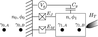
Figure 1: Setup corresponding to the model Hamiltonian Eq. (II), describing a superconducting island with charge $n$, superconducting phase $\phi_{1}$ and Majorana bound states $\gamma_{1,A/B}$ coupled to a ground superconductor with charge $n_{0}$, superconducting phase $\phi_{0}$ and Majorana bound states $\gamma_{0,A/B}$. The coupling is realized through a Josephson junction (depicted by a boxed cross) with Josephson energy $E_{J}$ and a Majorana-Josephson junction (depicted as a half-cross) between bound states $\gamma_{0,B}$ and $\gamma_{1,A}$ with coupling strength $E_{M}$. The island is coupled via a capacitance $C_{g}$ to a gate voltage $V_{g}$. The tunnel Hamiltonian $H_{T}$ denotes the possibility to couple the bound state $\gamma_{1,B}$ to a normalconducting tunneling tip.

Majorana fermions have attracted a lot of attention in the last years alicea:12 ; beenakker:13 due to their potential for quantum computation nayak:08 . At first sight, superconducting systems hosting Majorana fermions appear to be prime candidates for the realization of supersymmetry since they involve both bosonic (Cooper-pair condensate) and fermionic (Majorana fermions) degrees of freedom. Indeed, a supersymmetry in space-time has recently been shown to arise at an interface of two topological superconductors in two dimensions tsvelik:12 as well as at the quantum phase transition between a trivial and a topological superconductor in arbitrary dimensions grover:13 . In contrast, here we want to focus on a realization of supersymmetric quantum mechanics and its associated level degeneracies with the help of Majorana fermions that does not rely on their fermionic properties, but only on the simultaneous presence of an anomalous $4\pi$-periodic Josephson coupling and a normal one.

In Sec. II, we introduce our system of interest, the Majorana Cooper-pair box. In Sec. III, we give a short outline of supersymmetric quantum mechanics and show that the Majorana Cooper-pair box is supersymmetric for a certain ratio of Josephson to Majorana-Josephson coupling strength. In Sec. IV, we discuss a tunneling experiment for a direct probe of the level degeneracy predicted by the supersymmetry before we conclude by summarizing our main findings and discussing possible experimental realizations.

II Majorana Cooper-pair box

The system of interest is depicted in Fig. 1. It is based on the well-known Cooper-pair box, which consists of a superconducting island (with phase $\phi_{1}$) that is coupled to a ground superconductor (with phase $\phi_{0}$) via a gate voltage $V_{g}$ with capacitance $C_{g}$ and a Josephson junction with Josephson energy $E_{J}$. The Cooper-pair box is extended by a $4\pi$-periodic Josephson junction with coupling strength $E_{M}$ which is characteristic for topological superconductors. The $4\pi$-periodic Josephson effect comes along with one Majorana zero mode denoted by $\gamma_{0,B}$ and $\gamma_{1,A}$ on either side of the junction. Exchange of single electrons leads to the hybridization energy $iE_{M}\gamma_{0,B}\gamma_{1,A}\cos(\phi/2)$ where $\phi=\phi_{1}-\phi_{0}$ is the superconducting phase difference. Due to topological constraints, there are always an even number of Majorana zero modes on each superconducting island. Thus, we have to take into account two additional Majorana bound states $\gamma_{0,A}$ and $\gamma_{1,B}$. We assume that the Majorana modes on the same superconductor are sufficiently separated such that we can neglect the exponentially small energy splitting. In a specific realization of our proposed system, the Majorana bound states could be hosted, for example, at the ends of semiconductor nanowires placed on top of a conventional s-wave superconductor.oreg:10 ; lutchyn:10 However, our discussion is independent from the specific way the Majorana bound states are realized.

The total Hamiltonian of the system reads

$$H_{\gamma}=E_{C}(n-n_{g})^{2}+E_{J}\big{(}1-\cos\phi)$$

$$+iE_{M}\gamma_{0,B}\gamma_{1,A}\cos(\phi/2);$$ (1)

the last term is the Majorana Josephson coupling explained in details above. The first term is associated with the electrostatic charging energy $E_{C}=e^{2}/2C_{g}$ of having $n$ electrons on the superconducting island and $n_{g}=C_{g}V_{g}/e$ is the preferred electron number (with $e>0$ the elementary charge) on the island set by the gate voltage. The second term proportional to $E_{J}=\hbar I_{c}/2e$ arises due to the conventional Josephson coupling exchanging Cooper-pairs with a critical current $I_{c}$. In deriving the Hamiltonian, we have assumed a large ground superconductor such that there is no charging energy associated with it. As a result, the superconducting phase $\phi_{0}$ of the ground superconductor has no dynamics and we can choose a gauge with $\phi_{0}=0$. The number of electrons $n\in\mathbb{Z}$ and the phase $\phi_{1}=\phi$ of the superconducting island are conjugate variables and obey the angular-momentum algebra

$$[n,e^{\pm i\phi/2}]=\pm e^{\pm i\phi/2},$$ (2)

such that $e^{\pm i\phi/2}$ corresponds to addition/removal of a single electron. The Majorana operators obey the Clifford algebra

$$\{\gamma_{k},\gamma_{l}\}=\gamma_{k}\gamma_{l}+\gamma_{l}\gamma_{k}=2\delta_{kl}.$$ (3)

Assuming that the temperature is below the superconducting gap and that apart from the Majorana modes there are no additional Andreev states, an occupation of the (non-local) fermionic mode spanned by the Majorana bound states $\gamma_{1,A},\gamma_{1,B}$ must correspond to the presence of an odd number of electrons on the superconducting island. Consequently, we have the fermion parity constraintfu:10

$$i\gamma_{1,A}\gamma_{1,B}=(-1)^{n}$$ (4)

for the island and an analogous constraint for the ground superconductor. For each superconductor with a pair of Majorana bound states, the fermion parity constraint reduces the Hilbert space dimension by a factor of two, and consequently, the Hilbert space of the system (II) is four times smaller than one would naively expect. Since the Majorana degrees of freedom are slaved to the number operator $n$, they can be explicitly removed via a unitary transformation $U$, see App. A for details.heck:11 ; zazunov:11 We obtain

$$H=E_{C}(n-n_{g})^{2}+E_{J}(1-\cos\phi)+E_{M}\cos(\phi/2),$$ (5)

where $H$ is the projection of the transformed Hamiltonian $UH_{\gamma}U^{\dagger}$ onto the constraint surface. As the Hamiltonian is $4\pi$-periodic in $\phi$, the charge offsets $n_{g}$ are only defined modulo 1. Thus, we restrict ourselves to $n_{g}\in[-\tfrac{1}{2},\tfrac{1}{2}]$ and adjust $n$ accordingly. For the important situation with $n_{g}=0$, $n$ simply counts the number of excess charges. We will show that at this particular point the Hamiltonian (5) is supersymmetric with a level degeneracy due to the symmetry provided that $E_{M}=\sqrt{2E_{J}E_{C}}$.

III Supersymmetry

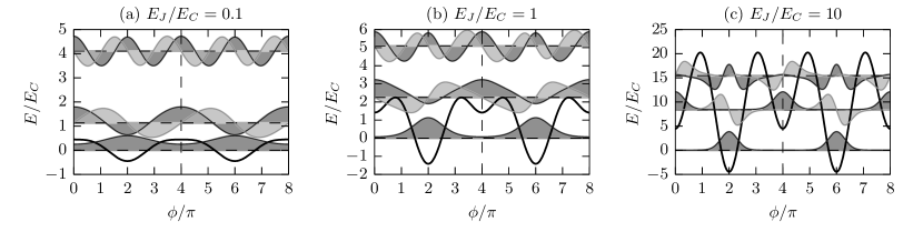
Figure 2: Numerically calculated wave functions $\psi_{n,\pm}(\phi)$ of the Hamiltonian Eq. (5) for $n=0,1,2$ at the supersymmetric point $n_{g}=0$, $E_{M}=\sqrt{2E_{J}E_{C}}$ for different values of $E_{J}/E_{C}$ (and thus $\alpha=\sqrt{2E_{J}/E_{C}}$). The wave functions are chosen real and are aligned at their corresponding eigenenergies. States $\psi_{n,+}(\phi)$ in the even parity sector of the superconducting phase are plotted in dark gray while the states $\psi_{n,-}(\phi)$ in the odd parity sector are plotted in light gray. The black line represents the underlying potential. Both the potential and the states are $4\pi$ periodic. We note that due to the supersymmetry, all levels with $n>0$ are doubly degenerate.

A supersymmetric Hamiltonian $H_{Q}$ decomposes into a direct sum of two terms that share the same spectrum up to a possibly missing ground state. The structure behind the $N=1$ supersymmetry in quantum mechanics is generated by a Hermitian supercharge $Q$ and Hermitian operator $K$ squaring to 1 which distinguishes the “bosonic” and “fermionic” sectors.combescure:04 In particular, these operators implement the algebra

$$\{Q,Q\} =2H_{Q}, \{Q,K\} =0,$$ (6)

which implies the conservation of $K$, $[H_{Q},K]=0$. The Hamiltonian decomposes into the eigenspaces of $K$ according to

$$H_{Q} =P_{+}H_{Q}P_{+}+P_{-}H_{Q}P_{-}, P_{\pm} =\tfrac{1}{2}(1\pm K).$$ (7)

Since the Hamiltonian is given by the square of a Hermitian operator, the eigenenergies are positive $E_{n}\geq 0$. Given an eigenstate $|n,+\rangle$ from the “bosonic” sector with eigenvalue $E_{n}>0$, the state $|n,-\rangle=Q|n,+\rangle/\sqrt{E_{n}}$ is an eigenvector of the “fermionic” sector with the same eigenvalue $E_{n}$.Note1

Showing that our system (5) is supersymmetric amounts to finding a supercharge $Q$ and an involution $K$ realizing the algebra Eq. (6). The first hunch that a potential supersymmetry might be related to the parity of the actual number of electrons on the superconducting island does not work due to the parity constraint (4), see App. B. However, the Majorana Cooper-pair box has a “hidden” supersymmetry as we will show in the following.

In order to show the supersymmetry of the Hamiltonian $H$ in the sense of Eq. (6), we have to define an operator $K$ characterizing the sectors which commutes with the Hamiltonian. For the special case $n_{g}=0$, such an operator is given by the parity $K:\phi\mapsto-\phi$ of the superconducting phase difference. We define the superchargeNote2

$$Q =\sqrt{E_{C}}\bigl{[}n-i\alpha\sin(\phi/2)\bigr{]}(-1)^{n}$$ (8)

$$=\sqrt{E_{C}}\{n(-1)^{n}+\tfrac{i\alpha}{2}[(-1)^{n}\sin(\tfrac{1}{2}\phi)-\sin(\tfrac{1}{2}\phi)(-1)^{n}]\},$$

where $\alpha$ is a free parameter and $(-1)^{n}$ is the fermion parity on the superconducting island. It is straightforward to check that $[(-1)^{n},K]=0$ and $\{n-i\alpha\sin(\phi/2),K\}=0$ such that $Q$ anticommutes with $K$.

Using the trigonometric relation $2\sin^{2}(\phi/2)=1-\cos\phi$, one obtains the supersymmetric Hamiltonian

$$H_{Q}=E_{C}\{n^{2}+\alpha\cos(\phi/2)+\tfrac{1}{2}\alpha^{2}[1-\cos(\phi)]\}$$ (9)

which for $\alpha=\sqrt{2E_{J}/E_{C}}$ is equal to the Hamiltonian (5) at the point

$$E_{M} =\sqrt{2E_{J}E_{C}}, n_{g} =0.$$ (10)

The supersymmetry leads to a degeneracy of the spectrum (apart from the ground state) which holds even in the nonperturbative regime of arbitrary $E_{J}/E_{C}$. While the supersymmetry presented here does not depend on the presence of fermionic degrees of freedom in the system, it relies crucially on the presence of an anomalous Josephson junction in addition to a conventional Josephson junction. In this sense it provides a clear signature of the Majorana-induced $4\pi$-periodic Josephson relation.

The supersymmetric structure of the Hamiltonian allows us to obtain the ground state(s) to the energy eigenvalue zero by solving the first-order differential equation $QP_{\pm}\psi_{0}(\phi)=0$ in the two sectors. In the present case, there is no solution to $QP_{-}\psi_{0}(\phi)=0$ since solutions to $Q\psi(\phi)=0$ are always even with respect to the parity $K$ of the superconducting phase difference. We obtain that the non-degenerate ground state at the supersymmetric point Eq. (10) is given by the function

$$\psi_{0}(\phi)=[4\pi I_{0}(2\alpha)]^{-1/2}\exp[-\alpha\cos(\phi/2)]$$ (11)

in the “bosonic” sector with the modified Bessel function $I_{0}(x)=\int_{0}^{2\pi}\!dt\,\exp(x\cos t)/2\pi$. All the excited states are doubly degenerate due to the supersymmetry. The algebraic construction of the higher energy levels and states is unfortunately not possible, since the potential is self-isospectral, that is identical in both sectors of the Hamiltonian, and the algebraic construction works only for potentials that differ in at least one parameter in the two sectors.cooper

Despite the lack of a general analytic solution for the degenerate excited states, we can still understand the degeneracy in the perturbative regimes. In particular, in the limit $\alpha\to 0$ we recover the supersymmetry of the free particle in one dimension as discussed by Ref. rau:04, . In this case the spectrum is given by $E_{n}=E_{C}n^{2}$ with the excess number of electrons $n\in\mathbb{Z}$; the ground state corresponds to $n=0$, and the level degeneracies are due to the two states $n$ and $-n$ at the same energy for $n\geq 1$.Note3 It is an instructive exercise to check that the level degeneracies persist when performing perturbation theory in $\alpha$. What can be observed is that each term in order $N$ involving $E_{J}$ cancels against a term in order $2N$ in $E_{M}$ appearing with opposite sign. Thus, the level degeneracy between $n$ and $-n$ persists to arbitrary order in $\alpha$, see Fig. 2. It is this particular cancellation of terms in the perturbation theory for which supersymmetry as a non-perturbative structure has been initially designed in the high-energy context.weinberg

In the semiclassical regime with $\alpha\to\infty$, the states are well localized close to the minima at $\phi\in 2\pi\mathbb{Z}$ where the potential $V=E_{M}\cos(\phi/2)+E_{J}(1-\cos\phi)$ can be expanded in quadratic order, see Fig. 2(c). Close to $\phi=2\pi$, we have $V_{2\pi}\approx-E_{M}+\tfrac{1}{2}E_{J}(\phi-2\pi)^{2}$ with the spectrum $E_{2\pi,n}=-E_{M}+\sqrt{8E_{C}E_{J}}(n+\tfrac{1}{2})$. In the second mimimum, at $\phi$ close to zero, we have $V_{0}\approx E_{M}+\tfrac{1}{2}E_{J}\phi^{2}$ which leads to the approximate spectrum $E_{0,n}=E_{M}+\sqrt{8E_{C}E_{J}}(n+\tfrac{1}{2})$. At the supersymmetric point (10), we observe the degeneracy $E_{2\pi,n+1}=E_{0,n}$ valid for $n\geq 0$. So the structure is again a single ground state $E_{2\pi,0}$ with degenerate levels above it. It is a highly nontrivial fact that the degeneracy found in the analysis above valid for $\alpha\to\infty$ remains intact for finite $\alpha$ where next order terms in the expansion of $V$ as well as tunneling events described by instantons have to been taken into account.

In the following, we will show that the degeneracies of the whole spectrum (except for the ground state) arising in the model (5) at the supersymmetric point can be directly probed by a tunneling experiment.

IV Tunneling current

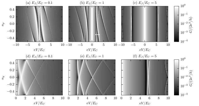
Figure 3: The differential tunneling conductance $G$ Eq. (15) at zero temperature at the special point $E_{M}=\sqrt{2E_{J}E_{C}}$ where the Hamiltonian of the system is supersymmetric for $n_{g}=0$. The conductances are plotted as a function of bias voltage $V$ and offset charge $n_{g}$ for different ratios $E_{J}/E_{C}$ of Josephson energy energy to the charging energy. It is calculated from the exact bare Green’s function $G^{R}_{0,\varepsilon}$ of the system computed by exact diagonalization and incorporating the leads via the Dyson equation (19) with a tunnel coupling $\Gamma=0.2E_{C}$. The upper panel displays the conductance $G(V)$ discriminating between electron and hole processes. The strong bias asymmetry at low $E_{J}/E_{C}$ reflects the transition from the charge basis to the phase basis as elaborated in the main text. The lower panel shows the symmetrized conductance $\tfrac{1}{2}[G(V)+G(-V)]$ which is easier to interpret. In the symmetrized conductance, the crossing of all the levels at $n_{g}=0$ is clearly visible. The white horizontal line in the upper panel (b) between $eV/E_{C}=1.2$ and $eV/E_{C}=3.5$ at $n_{g}=-0.3$ indicates the position of the line cut shown in Fig. 4.

To model the tunneling experiment depicted in Fig. 1, we assume that the system is coupled via the Hamiltonian

$$H_{T}=\sum_{p}w^{*}c_{p}^{\dagger}e^{-i\phi/2}\gamma_{1,B}+\text{H.c.},$$ (12)

to an effective noninteracting lead of spinless electrons described by the Hamiltonian $H_{L}=\sum_{p}\epsilon_{p}c_{p}^{\dagger}c_{p}$ with the fermionic annihilation operators $c_{p}$;Note4 here, $w$ is the tunneling matrix element and the presence of the operators $e^{\pm i\phi/2}$ account for the transfer of charge to the superconductor. For this setup, we derive in the App. C the exact expression

$$I=\frac{e\Gamma}{h}\int\!d\varepsilon\,(-\mathop{\rm Im}G^{R}_{\varepsilon})\left(2f_{\varepsilon-eV}-1\right)$$ (13)

for the tunneling current, see also Ref. hutzen:12, ; here, $f_{\varepsilon}=[1+\exp(\varepsilon/k_{B}T)]^{-1}$ is the Fermi distribution with respect to the chemical potential of the superconducting island and, consequently, $f_{\varepsilon-eV}$ is the distribution of the electrons in the lead. The tunnel coupling $\Gamma=2\pi|w|^{2}\rho_{0}$ is given in the wide-band limit where the electrons in the lead have the constant density of state $\rho_{0}$. The Majorana Green’s function in the presence of the leads is defined as

$$G^{R}_{\varepsilon}=-i\int_{0}^{\infty}\!dt\,e^{i\varepsilon t}\big{\langle}\bigl{\{}\tilde{\gamma}(t),\,\tilde{\gamma}^{\dagger}\bigr{\}}\big{\rangle},$$ (14)

with $\tilde{\gamma}=\gamma_{1,B}e^{-i\phi/2}$ evolving with respect to the full Hamiltonian $H_{\text{tot}}=H_{\gamma}+H_{L}+H_{T}$. From Eq. (13), the differential conductance $G(V)=dI/dV$ is obtained in the limit of low temperatures ($T\to 0$) where we can approximate $df_{\varepsilon}/d\varepsilon\approx-\delta(\varepsilon)$ as

$$G(V)=\frac{dI}{dV}=-\frac{2e^{2}\Gamma}{h}\mathop{\rm Im}G^{R}_{eV}.$$ (15)

Our goal is to evaluate the differential conductances in the tunneling limit $E_{J},E_{C}\gg\Gamma$. To this end, we need to relate the Majorana Green’s function $G^{R}_{\varepsilon}$ in presence of the leads to the Majorana Green’s function $G^{R}_{0,\varepsilon}$ without the leads ($w=0$) which can be evaluated by exact diagonalization.

In the non-interacting case ($E_{C}=0$), the retarded Majorana Green’s function obeys a Dyson equation in Nambu space,flensberg:10b which can be written as

$$\check{G}^{R}_{\varepsilon}=\check{G}_{0,\varepsilon}^{R}+\check{G}_{0,\varepsilon}^{R}\check{\Sigma}^{R}_{\varepsilon}\check{G}^{R}_{\varepsilon},$$ (16)

and where $\check{G}_{\varepsilon}$ is given by

$$\check{G}^{R}_{\varepsilon}=-i\int_{0}^{\infty}\!\!dt\,e^{i\varepsilon t}\Bigl{\langle}\begin{pmatrix}\{\tilde{\gamma}(t),\tilde{\gamma}^{\dagger}\}&\{\tilde{\gamma}(t),\tilde{\gamma}\}\\ \{\tilde{\gamma}^{\dagger}(t),\tilde{\gamma}^{\dagger}\}&\{\tilde{\gamma}^{\dagger}(t),\tilde{\gamma}\}\end{pmatrix}\Bigr{\rangle},$$ (17)

and

$$\check{\Sigma}^{R}_{\varepsilon} =|w|^{2}\sum_{p}\begin{pmatrix}(\varepsilon-\epsilon_{p}+i0^{+})^{-1}&0\\ 0&(\varepsilon+\epsilon_{p}+i0^{+})^{-1}\end{pmatrix}$$

$$=-\frac{i\Gamma}{2}\begin{pmatrix}1&0\\ 0&1\end{pmatrix}$$ (18)

is the self energy due to the lead. In the non-interacting limit ($E_{C}=0)$, the superconducting phase $\phi$ is constant, $\phi(t)=\phi(0)$, and thus all the four entries of the Green’s function $\check{G}^{R}_{\varepsilon}$ are equal. As a consequence, the Dyson equation becomes the scalar equation

$$G^{R}_{\varepsilon}=G_{0,\varepsilon}^{R}+G_{0,\varepsilon}^{R}\Sigma_{\varepsilon}^{R}G_{\varepsilon}^{R},$$ (19)

with the self energy $\Sigma^{R}_{\varepsilon}$ given by the sum of two processes corresponding to transitions of electron and holes to the lead,

$$\Sigma^{R}_{\varepsilon}=\mathop{\rm tr}(\check{\Sigma}^{R}_{\varepsilon})=-i\Gamma.$$ (20)

In the following, we assume that the scalar Dyson equation (19) remains applicable also in the interacting case. This corresponds to a decoupling at the sequential tunneling level and an inclusion of the leads through the self-energy (20). We thus neglect a potential difference in the dynamics between electrons and holes when tunneling to the lead.Note5 As explained in the App. D, the Green’s function $G_{0,\varepsilon}^{R}$ at $w=0$ can be expressed in the Lehmann representation as

$$G^{R}_{0,\varepsilon}=\sum_{k,\sigma}\frac{a_{k}^{\sigma}}{\varepsilon-\sigma E_{k0}+i0^{+}}$$ (21)

with the transition probabilities $a_{k}^{\sigma}=|\langle k|e^{i\sigma\phi/2}|0\rangle|^{2}$ to the exact eigenstate $|k\rangle$ of the Hamiltonian $H$ by adding ($\sigma=+$) or removing ($\sigma=-$) a single electron, where $E_{kl}=E_{k}-E_{l}$ are differences of the corresponding eigenenergies. The full retarded Green’s function $G^{R}_{\varepsilon}$ is obtained via the Dyson equation (19). The effect of the leads incorporated via the Dyson equation (19) is to provide a state-dependent broadening of the levels of the isolated system.

To get a feeling for the formulas, we first consider the simple situation where due to a large level separation only a single level $|k\rangle$ is close to resonance $eV\approx E_{k0}>0$. In this case, we can approximate $G_{0,\varepsilon}^{R}\approx a_{k}^{+}/(\varepsilon-E_{k0}+i0^{+})$. Resolving the Dyson equation and plugging the resulting expresssion for $G_{\varepsilon}^{R}$ into (15) yields

$$G(V)\approx\frac{2e^{2}}{h}\frac{(a_{k}^{+}\Gamma)^{2}}{(eV-E_{k0})^{2}+(a_{k}^{+}\Gamma)^{2}},$$ (22)

which describes a Lorentzian peak around the resonance energy $E_{k0}$ with level-dependent broadening $a_{k}^{+}\Gamma$ proportional to the probability of injecting an electron from the lead.

As a peak in the conductance is associated with the resonance condition $eV=E_{k0}$, we expect that the level degeneracy due to the supersymmetry is visible as a merging of two peaks when approaching the supersymmetric point. To test this hypothesis, we have numerically calculated the conductance by determining $G^{R}_{0,\varepsilon}$ via exact diagonalization of $H$ and subsequently resolving the Dyson equation (19). The resulting differential conductance Eq. (15) is displayed in Fig. 3 as a function of bias voltage and offset charge $n_{g}$. As was to be expected from the approximate expression Eq. (22), the conductance peaks with a value equal to the conductance quantum $2e^{2}/h$ when the bias voltage is tuned such that the chemical potential of the lead is in resonance with the eigenstates of the isolated system and resonant Andreev reflection occurs. The conductance plots exhibit the symmetry $G(V,n_{g})=G(-V,-n_{g})$ which is exact to our level of approximation. For the Hamiltonian $H$, a sign flip of the offset charge $n_{g}$ is equivalent to a sign flip of the superconducting phase under action of the parity operator $K:\phi\mapsto-\phi$. It is easily checked from the Lehmann representation Eq. (21) that $G_{0,\varepsilon}^{R}\mapsto-G_{0,-\varepsilon}^{A}$ under the operation of $K$ which due to the strucure of the Dyson equation (19) translates into $G(V)\mapsto G(-V)$. An intuitive reason for the symmetry $G(V,n_{g})=G(-V,-n_{g})$ is that the sign of $n_{g}$ favors an excess or defect number of electrons whereas the sign of $V$ corresponds to the lead preferably adding or removing electrons. As we have shown in Sec. III, the supersymmetry at small $E_{J}/E_{C}$ corresponds to a different sign of excess electrons. Thus the two levels that cross appear in the tunneling conductance at opposite bias. In order to remedy the problem that the crossing is not directly visible in the conductance as it appears at different bias, we plot the symmetrized conductance $\tfrac{1}{2}[G(V)+G(-V)]$ in the lower panel of Fig. 3 where the crossing of the levels at $n_{g}=0$ is visible for all ratios of $E_{J}$ to $E_{C}$. Due to the symmetry mentioned above, the plots of the symmetrized conductances are symmetric under $n_{g}\leftrightarrow-n_{g}$.

A striking feature which is especially visible in the unsymmetrized conductance plots is the coincidence of peaks in the conductances with regions of suppressed conductance. In Fig. 4, we have shown a linecut of the conductance as a function bias voltage $V$ at the point $E_{J}/E_{C}=1$, $E_{M}=\sqrt{2E_{J}E_{C}}$ and $n_{g}=-0.3$ for $\Gamma=0.2E_{C}$. It shows a sequence of two conductance peaks with their associated minima to the left of them. Each of the conductance maxima-minima pair has been fitted to a Fano resonances of the form

$$G_{\text{Fano}}(V)=\frac{2e^{2}}{h}\frac{(\beta\gamma/2+\varepsilon-\varepsilon_{0})^{2}}{(1+\beta^{2})[(\varepsilon-\varepsilon_{0})^{2}+\gamma^{2}/4]}$$ (23)

indicated by the dashed lines; here, $\beta\in\mathbb{R}$ is the asymmetry parameter, $\gamma$ is the line-width of the resonance, and $\varepsilon_{0}$ the position of the resonance. In the limit $|\beta|\rightarrow\infty$, the Fano resonance approaches the usual Breit-Wigner resonance. It is clear from Fig. 4 that the Fano-resonance behavior captures the behavior of the conductance close to the maximum.

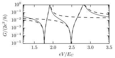
Figure 4: Solid line: Line cut through the tunneling conductance $G(V)$ shown in Fig. 3 for $E_{J}/E_{C}=1$, $E_{M}=\sqrt{2E_{J}E_{C}}$, $\Gamma=0.2E_{C}$ and $n_{g}=-0.3$ as a function of bias voltage $V$. Dashed lines: fits of Fano peaks of the form Eq. (23) with parameters $\beta=7.5$, $\gamma/E_{C}\approx 0.04$, $\varepsilon_{0}/E_{C}\approx 1.91$ for the resonance on the left and $\beta=6$, $\gamma/E_{C}\approx 0.11$, $\omega_{0}/E_{C}\approx 2.81$ for the resonance on the right.

.

In order to understand the microscopic origin of the Fano-like resonances, we study a simplified model with $E_{M}=0$ in the regime $E_{C}\gg E_{J}\gg\Gamma$. In this case, we can evaluate the Hamiltonian Eq. (5) in the charge basis and truncate to charge states $|n=0\rangle,|n=\pm 1\rangle$ which yields the effective three-level Hamiltonian

$$H\approx E_{J}+\begin{pmatrix}E_{C}(1+n_{g})^{2}&0&-E_{J}/2\\ 0&E_{C}n_{g}^{2}&0\\ -E_{J}/2&0&E_{C}(1-n_{g})^{2}\end{pmatrix}$$ (24)

with ground state $|0\rangle=|n=0\rangle$ at eigenenergy $E_{0}=E_{J}+E_{C}n_{g}^{2}$ (which is exact for all $E_{J}/E_{C}$ and $n_{g}$ due to the fact that we have set $E_{M}=0$) and excited states $|1,2\rangle$ with eigenenergies $E_{1,2}$.

Due to the algebra Eq. (2), we find $a^{\sigma}_{0}=|\langle 0|e^{\sigma i\phi/2}|0\rangle|^{2}=0$. The completeness relation leads to $a_{1}^{\sigma}+a_{2}^{\sigma}=1$. At the particle-hole symmetric point $n_{g}=0$, we have that $a_{1}^{\sigma}=a_{2}^{\sigma}=\tfrac{1}{2}$. For $n_{g}\neq 0$, the particle-hole symmetry is broken and thus $a_{1}^{\sigma}\neq a_{2}^{\sigma}$. The bare Green’s function $G_{0,\varepsilon}^{R}$ of the effective three-level system follows from the Lehmann representation Eq. (21). We consider the case of $V>0$ such that the main contribution arises from the terms with $\sigma=+$. Solving the Dyson equation for $G^{R}_{\omega}$, we obtain the expression

$$G(V)\approx\frac{2e^{2}}{h}\frac{(x-a_{1}^{+})^{2}}{(x-a_{1}^{+})^{2}+E_{21}^{2}x^{2}(1-x)^{2}/\Gamma^{2}}$$ (25)

for the conductance, where we have replaced the voltage by the dimensionless variable $x=(eV-E_{10})/E_{21}$ that is centered around the resonance at $eV=E_{10}$.Note6 Note that in the limit of large level-separation $x\to 0$, we recover the single-level conductance Eq. (22).

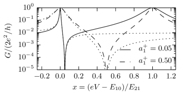
Figure 5: Differential tunneling conductance Eq. (25) into the effective three-level system Eq. (24) for $E_{21}/\Gamma=10$ and different values of the transition probability $a_{1}^{+}$ into the state $|1\rangle$. Dotted lines in the vicinity to the actual curves show the approximate Fano-resonance form Eq. (23) valid for $x=(\varepsilon-E_{10})/E_{21}\ll 1$ that is parametrized by $\beta=-E_{21}/\Gamma$, $\varepsilon_{0}=E_{10}+a_{1}^{+}E_{21}/(1+\beta^{2})$ and $\gamma=2a_{1}^{+}\Gamma\beta^{2}/(1+\beta^{2})$.

The new feature brought by the inclusion of the second level is a zero in the conductance for $\varepsilon$ between $E_{10}$ and $E_{20}$ at the position $x=a^{+}_{1}$.Note7 The zero in the conductance arises due to the competition of the processes of tunneling an electron into level $|1\rangle$ and level $|2\rangle$ leading to an interference. The interference can be traced back to the fact that the process happens at an energy $eV>E_{10}$ which is above the resonance at $E_{10}$ and thus is approximately phase shifted by $\pi$ with respect to the second level where $eV<E_{20}$. To see that the expression (25) of the differential conductance is of the Fano form close to the resonance at $x=0$, we expand $x$ to second order in the denominator and obtain $G_{\text{Fano}}(V)$ for the conductance around the resonance $E_{10}$, where $-\beta=E_{21}/\Gamma\gg 1$, $\gamma\approx 2a^{+}_{1}\Gamma$, and $\omega_{0}\approx E_{k0}$. Note that the asymmetry parameter $\beta$ is negative in accord with the fact that the root in the conductance occurs to the right of the resonance position $E_{10}$ and that $\gamma$ and $\omega_{0}$ fit the single level result (22). Since $\beta\gg 1$ in the tunneling regime, the zero is at a position where the conductance is already polynomially suppressed, but the dip in the conductance still clearly shows up in a logarithmic scale, cf. Fig. 4. For $E_{C}\gg E_{J}$, we have $a^{+}_{2}\rightarrow 0$ and we find a very sharp resonance at $E_{20}$ with dip in the conductance in close vicinity to $E_{20}$ (as compared to the peak separation $E_{21}$) whereas the resonance at $E_{10}$ assumes its usual Breit-Wigner form, see Fig. 5. It is interesting to note that similar interference effects are known from transport through molecules when multiple transport channels are available.guedon:12 ; geranton:13

V Conclusions

We have shown that the extension of the usual Cooper-pair box by a Majorana-Josephson junction features a degeneracy in its spectrum for $n_{g}=0$ and $E_{M}=\sqrt{2E_{J}E_{C}}$ that is due to a “hidden” bosonic supersymmetry generalizing the supersymmetry of the free particle. The supersymmetry crucially relies on the presence of the anomalous Josephson junction and an observation of the predicted level crossings of all excited states at the supersymmetric point provides a clear indication of the presence of a Majorana-induced anomalous Josephson junction.

We have shown that the supersymmetry can be probed directly in a tunneling experiment by varying the bias voltage $V$ and the offset charge $n_{g}$. In the tunneling regime, when the bias voltage is tuned such that the Fermi level of the lead coincides with the eigenenergies of the isolated system, resonant Andreev reflection with a peak conductance equal to the conductance quantum $2e^{2}/h$ occurs for the whole range of $E_{J}/E_{C}$ values. The crossing of all excited eigenstates of the system as the supersymmetric point is approached can thus clearly be observed in conductance maps obtained by varying the offset charge $n_{g}$ and gate voltage $V$. The conductance features suppressed conductance close to the resonances that are due to interference. We have explained that the interference is due the presence of several channels for single-electron tunneling which exist since the island charge is not a sharp observable by considering a simple analytic model in the regime $E_{J}/E_{C}\ll 1$.

Interestingly, the supersymmetry presented here could also be found in Josephson Rhombi chains allowing tunneling of pairs of Cooper pairsdoucot:02 in addition to conventional Cooper-pair tunneling that are constructed in conventional Josephson junction arrays and have recently been realized experimentally.bell:13 However, in this case the Hilbert space only involves the superconducting condensate and the states and potential degeneracies of the system cannot be simply probed by tunneling spectroscopy as proposed in this paper. It is an interesting question for future work, if there is a simple experimental signature of supersymmetry in this setup.

Appendix A Bosonization of the Hamiltonian

Bosonizing the Majorana operators of the Hamiltonian Eq. (II) via a Jordan-Wigner transformation as

$$\gamma_{k,A} =\Big{(}\prod_{l<k}\,\sigma_{l}^{z}\Big{)}\sigma_{k}^{x} \gamma_{k,B} =-\Big{(}\prod_{l<k}\,\sigma_{l}^{z}\Big{)}\sigma_{k}^{y},$$ (26)

where $\sigma_{k}^{x,y,z}$ are independent sets of Pauli-matrices for each index $k$, brings the Majorana tunneling term to the form

$$E_{M}\sigma_{0}^{x}\sigma_{1}^{x}\cos(\phi/2)=E_{M}\cos((\phi+\pi\sigma_{0}^{x}-\pi\sigma_{1}^{x})/2).$$ (27)

Performing a unitary transformation $U=\prod_{k=0,1}U_{k}$ with

$$U_{k}=e^{-i\pi\sigma_{k}^{x}n_{k}/2}=\cos(\pi n_{k}/2)-i\sigma_{k}^{x}\sin(\pi n_{k}/2),$$ (28)

which links the transfer of one electron to a flip of the fermion parity and where we use the notation $n_{1}=n$, the transformed Hamiltonian assumes the form

$$UH_{\gamma}U^{\dagger}=\Big{\{}E_{C}(n-n_{g})^{2}+E_{J}(1-\cos\phi)$$

$$+E_{M}\cos(\phi/2)\Big{\}}I,$$ (29)

while the fermion parity constraint Eq. (4) is transformed into

$$\cos(\pi n_{k})\sigma_{k}^{z}-\sin(\pi n_{k})\sigma_{k}^{y}=(-1)^{n_{k}}.$$ (30)

In Eq. (29), we have made explicit the trivial remaining spin-structure of the Hamiltonian. On the other hand, the transformed constraint fixes integer charges $n_{k}\in\mathbb{Z}$ and enforces spin-up eigenstates of $\sigma_{k}^{z}$. The fermion-parity constraint is thus resolved in the transformed Hamiltonian Eq. (29) by considering just one spin-component and demanding a $4\pi$ periodicity of the eigenstates, leading to the Hamiltonian Eq. (5) given in the main text.

Appendix B Supersymmetry without the fermion parity constraint

In a theory not bound by the fermion parity constraint Eq. (4), the fermion parity $K^{\prime}=i\gamma_{0,B}\gamma_{1,A}$ across the Majorana junction is easily seen to be conserved in the original Hamiltonian $H_{\gamma}$ from Eq. (II). The natural choice for the supercharge $Q^{\prime}$ is then given by

$$Q^{\prime}=\sqrt{E_{C}}\bigl{[}(n-n_{g})\,\gamma_{0,B}-\alpha^{\prime}\sin(\phi/2)\gamma_{1,A}\bigr{]},$$ (31)

where $\alpha^{\prime}$ is a free parameter. The charge $Q^{\prime}$ anticommutes with the fermion parity $K^{\prime}$ across the junction. One verifies that $Q^{\prime 2}=H_{\gamma}$ for the parameters Eq. (10) given in the main text and $\alpha^{\prime}=\alpha=\sqrt{2E_{J}/E_{C}}$. The supersymmetry described above corresponds to a supersymmetry between bosonic and fermionic sectors, which cannot be realized in our system since the Majoranas are no longer an independent degree of freedom due to the fermion parity constraint Eq. (4) and only the bosonized “hidden” supersymmetry given in the main text remains.

Appendix C Derivation of the current

Let us define a generic tunneling Hamiltonian

$$H_{T}=\sum_{ilp}w_{lpi}^{*}c_{lp}^{\dagger}e^{-i\phi_{i}/2}\gamma_{k}+w_{lpi}\gamma_{i}e^{i\phi_{i}/2}c_{lp},$$ (32)

describing the tunneling with tunneling matrix elements $w_{lpi}$ between electrons of momentum $p$ in lead $l$ with creation/annihilation operators $c_{lp}^{\dagger},c_{lp}$ into Majorana bound states $\gamma_{i}$ with associated superconducting phases $\phi_{i}$ ($\phi_{i}=\phi_{j}$ for Majoranas on the same superconductor). The leads are free with Hamiltonian

$$H_{L}=\sum_{l}\sum_{p}\epsilon_{lp}c_{lp}^{\dagger}c_{lp}.$$ (33)

Defining operators $\tilde{\gamma}_{i}=e^{-i\phi_{i}/2}\gamma_{i}$, the tunneling Hamiltonian has the appearance of a standard fermionic tunneling Hamiltonian. It is well-known [][; Chap.12.4;]haug; *[][; Chap.8.9]datta that the expression for the steady-state current $I_{l}$ through lead $l$, given a system with a tunneling Hamiltonian of the form Eq. (12) and non-interacting leads, can always be cast in the form

$$I_{l}=\frac{e}{\hbar}\int\frac{d\varepsilon}{2\pi}\mathop{\rm tr}\big{[}(iG_{\varepsilon}^{>})\Gamma_{\varepsilon}^{l}f^{l}_{\varepsilon}-(-iG_{\varepsilon}^{<})\Gamma_{\varepsilon}^{l}(1-f_{\varepsilon}^{l})\big{]},$$ (34)

where only the non-interaction of the leads has been exploited and

$$(G^{<}_{\varepsilon})_{ij} =i\int dt\,e^{i\varepsilon t}\,\big{\langle}\tilde{\gamma}_{j}^{\dagger}\tilde{\gamma}_{i}(t)\big{\rangle}$$ (35)

$$(G^{>}_{\varepsilon})_{ij} =-i\int dt\,e^{i\varepsilon t}\,\big{\langle}\tilde{\gamma}_{i}(t)\tilde{\gamma}_{j}^{\dagger}\big{\rangle}$$ (36)

are the lesser/greater Majorana Green’s functions in presence of the leads in the steady state limit, $f^{l}_{\varepsilon}$ is the equilibrium Fermi distribution of lead $l$ and $(\Gamma_{\varepsilon}^{l})_{ij}=2\pi\sum_{p}w_{lpi}w_{lpj}^{*}\delta(\varepsilon-\epsilon_{lp})$ is the lead coupling matrix. The current expression Eq. (34) has a straight-forward interpretation: the contribution to the current through lead $l$ at energy $\varepsilon$ is given by the rate $\Gamma_{\varepsilon}^{l}f_{\varepsilon}^{l}$ of electron tunneling into the system through lead $l$ at energy $\varepsilon$ times the number $iG^{>}_{\varepsilon}$ of available states at this energy minus the rate $\Gamma_{\varepsilon}^{l}(1-f_{\varepsilon}^{l})$ of electrons tunneling out of the system into lead $l$ times the number $-iG^{<}_{\varepsilon}$ of occupied states.[][; Chap.8.9]datta With the Keldysh Green’s function $G^{K}=G^{>}+G^{<}$ and the relation $G^{R}-G^{A}=G^{>}-G^{<}$, one can rewrite the expression Eq. (34) in the form

$$I_{l} =\frac{e}{\hbar}\int\frac{d\varepsilon}{2\pi}\mathop{\rm tr}\Big{\{}\big{[}i(G_{\varepsilon}^{R}-G_{\varepsilon}^{A})+iG^{K}_{\varepsilon}\big{]}\Gamma_{\varepsilon}^{l}f_{\varepsilon}^{l}$$

$$\qquad-\big{[}i(G_{\varepsilon}^{R}-G_{\varepsilon}^{A})-iG^{K}_{\varepsilon}\big{]}\Gamma_{\varepsilon}^{l}(1-f_{\varepsilon}^{l})\Big{\}}$$ (37)

$$=\frac{e}{\hbar}\int\frac{d\varepsilon}{2\pi}\mathop{\rm tr}\Big{\{}i(G_{\varepsilon}^{R}-G_{\varepsilon}^{A})\Gamma_{\varepsilon}^{l}(2f^{l}_{\varepsilon}-1)$$

$$\qquad+\frac{i}{2}G^{K}_{\varepsilon}\Gamma_{\varepsilon}^{l}\Big{\}}.$$ (38)

The key observation from Ref. hutzen:12, is that the $G_{\varepsilon}^{K}$ expression vanishes when working with a wide band, $\Gamma^{l}_{\varepsilon}=\Gamma^{l}$, and assuming coupling to just one Majorana $\gamma_{k}$, $(\Gamma^{l})_{ij}=(\Gamma^{l})_{kk}\delta_{ik}\delta_{jk}$, i.e.,

$$0=\int\frac{d\varepsilon}{2\pi}\mathop{\rm tr}[G_{\varepsilon}^{K}\Gamma_{\varepsilon}^{l}]=(\Gamma^{l})_{kk}G^{K}(t=0)_{kk}$$ (39)

since $G^{K}(t=0)_{kk}=-i\big{\langle}[\tilde{\gamma}_{k},\tilde{\gamma}_{k}^{\dagger}]\big{\rangle}=0$. Thus, in the wide-band limit with coupling to just one Majorana $\gamma_{k}$, one obtains the expression

$$I_{l}=\frac{e}{\hbar}\int\frac{d\varepsilon}{2\pi}\big{(}-\mathop{\rm Im}G_{\varepsilon}^{R}\big{)}_{kk}(\Gamma^{l})_{kk}(2f^{l}_{\varepsilon}-1),$$ (40)

valid both in non-interacting and interacting setups. The very cumbersome feature brought by the Majoranas is that even in the interacting case the current expression remains completely independent from the occupation state of the system and depends only on spectral properties. This can be seen as yet another reflection of the fact that a single Majorana mode does not have a well-defined occupation number.

Appendix D Evaluation of transition probabilities

The eigenstates $|k_{\gamma}\rangle$ of the Hamiltonian $H_{\gamma}$ from Eq. (II) are related to the eigenstates $|k\rangle$ of the bosonized Hamiltonian $H$ from Eq. (5) via the unitary transformation Eq. (28) as $|n\rangle=U|n_{\gamma}\rangle$. The Majorana $\gamma_{1,B}$ is in the bosonized form expressed as $\gamma_{1,B}=-\sigma_{0}^{z}\sigma_{1}^{y}$. Using $U\sigma_{k}^{y}U^{\dagger}=(-1)^{n_{k}}\sigma_{k}^{y}$, $U\sigma_{k}^{z}U^{\dagger}=(-1)^{n_{k}}\sigma_{k}^{z}$ and $Ue^{\pm i\phi_{k}/2}U^{\dagger}=\mp i\sigma_{k}^{x}e^{\pm i\sigma_{k}^{x}/2}$, where we again identify $n_{1}=n$, one finds

$$U\gamma_{1,B}e^{\pm i\phi/2}U^{\dagger}=\mp\sigma_{0}^{z}\sigma_{1}^{z}e^{\pm i\phi/2}(-1)^{n_{0}+n}.$$ (41)

Since $n_{0}+n$ and $\sigma_{k}^{z}$ are conserved quantities of the Hamiltonian Eq. (29), one obtains for the transition probabilites $|\langle k_{\gamma}|\gamma_{1,B}e^{\pm i\phi/2}|l_{\gamma}\rangle|^{2}$ the result

$$|\langle k_{\gamma}|\gamma_{1,B}e^{\pm i\phi/2}|l_{\gamma}\rangle|^{2}=|\langle k|e^{\pm i\phi/2}|l\rangle|^{2}$$ (42)

employed in the main text.

References

- (1) E. Witten, Nucl. Phys. B 188 (3), 513 (1981).
- (2) F. Cooper and B. Freedman, Ann. Phys. (NY) 146 (2), 262 (1983).
- (3) F. Cooper, A. Khare, and U. Sukhatme, Phys. Rep. 251 (5-6), 267 (1995).
- (4) P. Fendley, B. Nienhuis, and K. Schoutens, J. Phys. A 36, 12399 (2003).
- (5) P. Fendley, K. Schoutens, and J. de Boer, Phys. Rev. Lett. 90, 120402 (2003).
- (6) M. Beccaria and G. F. De Angelis, Phys. Rev. Lett. 94, 100401 (2005).
- (7) L. Huijse, J. Halverson, P. Fendley, and K. Schoutens, Phys. Rev. Lett. 101, 146406 (2008).
- (8) R. D. Tangerman and J. A. Tjon, Phys. Rev. A 48, 1089 (1993).
- (9) M. Snoek, M. Haque, S. Vandoren, and H. T. C. Stoof, Phys. Rev. Lett. 95, 250401 (2005).
- (10) Y. Yu and K. Yang, Phys. Rev. Lett. 100, 090404 (2008).
- (11) M. S. Plyushchay, Mod. Phys. Lett. A 11, 397 (1996).
- (12) A. R. P. Rau, J. Phys. A 37, 10421 (2004).
- (13) J. Alicea, Rep. Prog. Phys. 75, 076501 (2012).
- (14) C. W. J. Beenakker, Annu. Rev. Con. Mat. Phys. 4, 113 (2013).
- (15) C. Nayak, S. H. Simon, A. Stern, M. Freedman, and S. Das Sarma, Rev. Mod. Phys. 80, 1083 (2008).
- (16) A. M. Tsvelik, Europhys. Lett. 97, 17011 (2012).
- (17) T. Grover, D. N. Sheng, and A. Vishwanath, arXiv:1301.7449 (2013).
- (18) Y. Oreg, G. Refael, and F. von Oppen, Phys. Rev. Lett. 105, 177002 (2010).
- (19) R. M. Lutchyn, J. D. Sau, and S. Das Sarma, Phys. Rev. Lett. 105, 077001 (2010).
- (20) L. Fu, Phys. Rev. Lett. 104, 056402 (2010).
- (21) B. van Heck, F. Hassler, A. R. Akhmerov, and C. W. J. Beenakker, Phys. Rev. B 84, 180502(R) (2011).
- (22) A. Zazunov, A. L. Yeyati, and R. Egger, Phys. Rev. B 84, 165440 (2011).
- (23) M. Combescure, F. Gieres, and M. Kibler, J. Phys. A 37, 10385 (2004).
- (24) Note that only when the sign of corresponds to the parity of physical fermions in the system, the resulting structure is a true supersymmetry between bosons and fermions. In general, the symmetry of the Hamiltonian is not in any way related to actual fermions or bosons present in the system.
- (25) In going from the first to the second line, we have used the fact that anticommutes with as the latter creates transitions between different fermion parity states.
- (26) F. Cooper, A. Khare, and U. Sukhatme, Supersymmetry in Quantum Mechanics (World Scientific, 2001).
- (27) We obtain the free particle spectrum by the relation with the mass of the particle and the length of of the system.
- (28) S. Weinberg, The Quantum Theory of Fields: Supersymmetry, The Quantum Theory of Fields (Cambridge University Press, 2000).
- (29) If the leads are spin-degenerate, only one of the Kramers’ partners is coupled to the Majorana mode while the other is completely reflected and thus our results remain valid in this case.
- (30) R. Hützen, A. Zazunov, B. Braunecker, A. L. Yeyati, and R. Egger, Phys. Rev. Lett. 109, 166403 (2012).
- (31) K. Flensberg, Phys. Rev. B 82, 180516(R) (2010).
- (32) Alternatively, one could work with the Nambu-Dyson equation (16), which contains the different dynamics through the anomalous Green’s functions of type , . We have checked that this does not qualitatively alter the results and thus we proceed with the simpler approach, i.e., the decoupling given in the main text.
- (33) The conductance can also be expressed as a function of centered around the second resonance at through the symmetry and which can be used for the analysis of the expression close to .
- (34) That the conductance is exactly zero is an artifact of the restricted Hilbert space. In general, the zero is replaced by a suppression of the conductance.
- (35) C. M. Guédon, H. Valkenier, T. Markussen, K. S. Thygesen, J. C. Hummelen, and S. J. van der Molen, Nat. Nanotech. 7 (5), 305 (2012).
- (36) G. Géranton, C. Seiler, A. Bagrets, L. Venkataraman, and F. Evers, J. Chem. Phys. 139 (23), 234701 (2013).
- (37) B. Doucot and J. Vidal, Phys. Rev. Lett. 88, 227005 (2002).
- (38) M. T. Bell, J. Paramanandam, L. B. Ioffe, and M. E. Gershenson, arXiv:1311.6521 (2013).
- (39) H. Haug and A. Jauho, Quantum Kinetics in Transport and Optics of Semiconductors, Solid-State Sciences (Springer, 2007).
- (40) S. Datta, Electronic Transport in Mesoscopic Systems (Cambridge University Press, Cambridge, 1995).