Magnetic field distribution and characteristic fields of the vortex lattice for a clean superconducting niobium sample in an external field applied along a three-fold axis

Abstract

The field distribution in the vortex lattice of a pure niobium single crystal with an external field applied along a three-fold axis has been investigated by the transverse-field muon-spin-rotation (TF-$\mu$SR) technique over a wide range of temperatures and fields. The experimental data have been analyzed with the Delrieu’s solution for the form factor supplemented by phenomenological formulas for the parameters. This has enabled us to experimentally establish the temperatures and fields for the Delrieu’s, Ginzburg-Landau’s, and Klein’s regions of the vortex lattice. Using the numerical solution of the quasiclassical Eilenberger’s equation the experimental results have been reasonably understood. They should apply to all clean BCS superconductors. The analytical Delrieu’s model supplemented by phenomenological formulas for its parameters is found to be reliable for analyzing TF-$\mu$SR experimental data for a substantial part of the mixed phase. The Abrikosov’s limit is contained in it.

I Introduction

The physical properties of superconductors are usually described by the phenomenological Ginzburg-Landau (GL) theory.Tinkham (1996); Ketterson and Song (1999) For a type-II superconductor it predicts a mixed phase with a periodic variation of the magnetic induction in the form of a vortex lattice (VL), as first derived by Abrikosov.Abrikosov (1957) For a simple superconductor the VL is characterized by three fields: the minimum field, the field at the saddle point of the field map, and the maximum field which is found in the vortex cores. The minimum field lies at the centre of the equilateral triangle formed by three nearest neighbor vortex cores. This simple picture is believed to be valid, although the GL’s theory is theoretically justified only in the vicinity of $T_{\rm c0}$,Gor’kov (1959) the critical temperature at low field. However, because of its simplicity, it serves as a basis for data analysis of experiments performed in the whole mixed phase.Sonier et al. (2000); Sonier (2007)

Using an approximate solution of the microscopic BCS-Gor’kov’s equation,Gor’kov (1959) Delrieu discovered the minimum field in the vicinity of the upper critical field $B_{\rm c2}$ at low temperature to be at the midpoint between two vortex cores.Delrieu (1972) Later on, solving numerically the Eilenberger’s equation Eilenberger (1968) — an analytical approximation to the BCS-Gor’kov’s equation involving an integration over the magnitude of the electron wave vector — Klein found two field minima in the VL unit cell at intermediate temperature.Klein (1987) Consistent with Klein’s results, nuclear magnetic resonance (NMR) experiments by Kung Kung (1970) on vanadium have detected a linear temperature dependence of the vortex-core field in a large temperature range towards zero temperature.

Here we present an exhaustive study of the field distribution in the VL of a pure niobium single crystal with the magnetic field ${\bf B}_{\rm ext}$ applied along a crystallographic $\langle 111\rangle$ direction. The measurements have been done using the transverse-field positive-muon-rotation (TF-$\mu$SR) technique.Dalmas de Réotier and Yaouanc (1997); Yaouanc and Dalmas de Réotier (2011) We have recently published a report which focuses on the $B_{\rm c2}$ vicinity.Maisuradze et al. (2013) The present data have been analyzed with an expression for the form factor derived analytically by Delrieu. Notice that the form factor of Abrikosov is a limiting case of the former expression. Combining experimental and theoretical results, we have established the VL characteristics predicted by Abrikosov, Delrieu and Klein in the proper parameter ranges. Our findings have been explained semi quantitatively using results obtained by solving numerically the Eilenberger’s equation assuming a cylindrical Fermi surface.

The organization of this paper is as follows. Section II introduces theoretical models for the VL field distribution. In Sec. III the sample is described, as well as the experimental conditions and the data analysis. Section IV displays typically measured field distributions. The following section (Sec. V) discusses the VL characteristics derived from the present experimental and theoretical studies. We summarize the results obtained in this work in Section VI. Possible improvements of the data analysis and experimental conditions are mentioned. Some conclusions and perspectives are presented in Sec. VII.

The reader only interested by the characteristics of the VL for niobium derived from our measurements and their analysis will jump directly to Sec. V. We stress that they are expected to be found for all clean BCS superconductors.

II Theoretical background on the field distribution in the VL of niobium

We shall first shortly describe the theories used to fit the $\mu$SR asymmetry time spectra. Then we shall present some computed field distributions.

We recall that a conventional triangular VL is observed when ${\bf B}_{\rm ext}$ is applied along a three-fold axis as revealed by small-angle neutron scattering (SANS).Schelten et al. (1971); Kahn and Parette (1973); Forgan et al. (2002); Mühlbauer et al. (2009) In contrast to expectation, the VL field distribution is not described by the GL theory for $B_{\rm ext}$ in the $B_{\rm c2}$ vicinity at low temperature.Herlach et al. (1990); Maisuradze et al. (2013) On the other hand, the approximate Delrieu’s solution of the BCS-Gor’kov equation explains the measured distribution, but only above 0.6 K.Maisuradze et al. (2013) This is a temperature much lower than the zero field critical temperature $T_{\rm c0}=9.25$ K.

II.1 Description of the available theories

We illustrate in Fig. 1 an equilateral triangular VL.

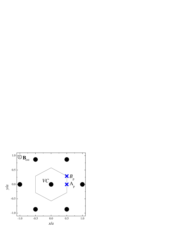
Figure 1: (color online). A triangular vortex lattice in the direct space. The external field ${\bf B}_{\rm ext}$ is applied perpendicular to the vortex plane. The bullets illustrate vortex core coordinates and the crosses two positions of particular interest in a unit cell, $A_{\rm p}$ and $B_{\rm p}$. In addition, we specify the position of one of the vortex core center with $VC$ nearby. The thin solid line represents the Wigner-Seitz cell. The position coordinates are scaled by the VL parameter $a$.

Three positions of special interest have been defined: the midpoint between two consecutive vortex cores, i.e. $A_{\rm p}$, and the centre of an equilateral triangle formed by three nearest neighbor vortex cores, i.e. $B_{\rm p}$. In addition, a vortex-core position is labeled as $VC$.

The TF-$\mu$SR technique gives access to the component field distribution along the ${\bf B}_{\rm ext}$ direction if $B_{\rm ext}$ is sufficiently large.Yaouanc and Dalmas de Réotier (2011) This is the case here. Labeling this direction as $Z$, ${\tilde{D}}_{\rm c}(B^{Z})$ is measured. It can be computed from the real space field map $B^{Z}({\bf r})$ of the two-dimensional VL:

$${\tilde{D}}_{\rm c}(B^{Z})=\int_{\rm u.c.}\delta(B^{Z}({\bf r})-B^{Z}){\rm d}^{2}{\bf r},$$ (1)

where the integral extends over the VL unit cell. In terms of its Fourier components $B^{Z}_{{\bf K}_{m,n}}$, we have for the field map

$$B^{Z}({\bf r})=\sum_{{\bf K}_{m,n}}B^{Z}_{{\bf K}_{m,n}}\exp(i{{\bf K}_{m,n}}\cdot{\bf r}),$$ (2)

where the sum is over the reciprocal space of the VL.

We need an expression for $B^{Z}_{{\bf K}_{m,n}}$ which is usually called the form factor in the SANS literature.

First of all we note that our sample is in the clean limit.Maisuradze et al. (2013) So we do not need to consider the effect of impurities. We shall use two theories for the computation of $B^{Z}_{{\bf K}_{m,n}}$ that are approximations to the BCS-Gor’kov theory. Two types of approximations are to be considered: the ones common and the ones particular to a theory. Common is the semiclassical approximation. Here the hypothesis is made that the spacing between the Landau levels is small in comparison to the sum of their thermal and collision broadenings.Werthamer (1969) This is expected to be valid for niobium down to $\approx 0.04$ K.Maisuradze and Yaouanc (2013) To get quantitative predictions to compare with experimental data, we need a simple, but still realistic, Fermi surface. The Delrieu’s solution of the BCS-Gor’kov equation assumes a spherical Fermi surface. For an extensive numerical study of the Eilenberger’s equation such as presented here, a cylindrical Fermi surface is a natural choice. This is partly because of computational convenience and is believed to be enough for the present purpose to constructing the phase diagram. Its essential features and other properties in this paper do not change when a 3-dimensional Fermi surface model is used, merely changing the $\kappa_{\rm GL}$ value. We can translate and interpret the $\kappa_{\rm GL}$ values between the 2-dimensional and 3-dimensional cases. As for more realistic Fermi surface models, some of us have an experience to use a realistic 3-dimensional Fermi surface model calculated by band theory for niobium.Adachi et al. (2011) In order to evaluate the subtle vortex lattice orientational changes for ${\bf B}_{\rm ext}\parallel\langle 001\rangle$ it is definitely needed to have a realistic Fermi surface model. For the present purposes the cylindrical Fermi surface model is believed to be enough.

Next, for completeness we summarize the work of Delrieu. He neglected the spatial dependence of the order parameter $\Delta({\bf r})$. While this approximation is reasonable in the vicinity of $B_{\rm c2}$, it should break down when approaching the lower critical field. He derived $B^{Z}_{{\bf K}_{m,n}}=f_{m,h}({\tilde{a}},{\tilde{b}},{\tilde{c}})$. The function $f_{m,h}$ can be found elsewhere.Delrieu (1972); Maisuradze and Yaouanc (2013) Here ${\tilde{a}}$ has the dimension of a field:

$${\tilde{a}}=-{\mu_{0}N_{0}\Delta^{2}_{0}\over 2{\overline{B^{Z}}}}{\tilde{c}}.$$ (3)

In the region of validity of the Delrieu’s approximation, $\overline{B^{Z}({\bf r})}\equiv\overline{B^{Z}}\simeq B_{\rm ext}$. The parameter ${\tilde{a}}$ does not influence the shape of $B^{Z}_{{\bf K}_{m,n}}$ and therefore ${\tilde{D}}_{\rm c}(B^{Z})$. It only gives its scale. It is proportional to the density of state at the Fermi level in the normal metal $N_{0}$ (per spin, volume, and energy), the quantity $\Delta^{2}_{0}=\overline{|\Delta({\bf r})|^{2}}$ ($\overline{|\Delta({\bf r})|^{2}}$ is the spacial average of $|\Delta({\bf r})|^{2}$), and is inversely proportional to the average field $\overline{B^{Z}}$. The dimensionless parameters ${\tilde{b}}$ and ${\tilde{c}}$ determine the ${\tilde{D}}_{\rm c}(B^{Z})$ shape and are expressed in terms of the ratios of three length scales: ${\tilde{b}}=[\Lambda/(\pi\xi^{B})]^{2}$ and ${\tilde{c}}=\Lambda/\xi^{T}$. Here, $\Lambda=[\Phi_{0}/(2\pi\overline{B^{z}}]^{1/2}$ is a length parameter proportional to the intervortex distance. The field and temperature dependent length scale $\xi^{B}=\hbar v_{\rm F}/(\pi\Delta_{0})$ diverges near $B_{\rm c2}$, while $\xi^{T}=\hbar v_{\rm F}/(2\pi k_{\rm B}T)$. We have introduced the Fermi velocity $v_{\rm F}$. It is easily found that

$${\tilde{b}}={1\over\pi^{2}}{\xi^{2}_{\rm GL}(T)\over\xi^{2}_{0}(T)}{1-b\over b},$$ (4)

where $b=B_{\rm ext}/B_{c2}(T)$ is the reduced field, $\xi_{\rm GL}$ the GL coherence length, and $\xi_{0}$ Pippard-BCS coherence length.Maisuradze and Yaouanc (2013) To derive Eq. 4 two phenomelogical formulas expected to be valid for conventional superconductors have been used:

$$\Delta_{0}=\Delta_{0}(0)\sqrt{1-b}\sqrt{1-\tau^{2}},$$ (5)

and

$$B_{\rm c2}(T)=B_{\rm c2}(0)(1-\tau^{2}),$$ (6)

where $\tau=T/T_{\rm c0}$. Since ${\xi^{2}_{\rm GL}(T)\over\xi^{2}_{0}(T)}={\xi^{2}_{\rm GL}(0)\over\xi^{2}_{0}(0)}$ and ${\xi_{\rm GL}(0)\simeq\xi_{0}(0)/0.96}$ in the clean limit,Tinkham (1996)

$${\tilde{b}}=0.110{1-b\over b}.$$ (7)

Hence, ${\tilde{b}}$ only depends on $b$. The parameter ${\tilde{c}}$ can be expressed in terms of $v_{\rm F}$:Maisuradze and Yaouanc (2013)

$${\tilde{c}}={\sqrt{\Phi_{0}2\pi}k_{\rm B}T\over\sqrt{\overline{B^{Z}}}\hbar v_{\rm F}},$$ (8)

where $\Phi_{0}$ is the magnetic flux quantum. Interestingly, $N_{0}\Delta_{0}^{2}$ in Eq. 3 is the condensation energy $E_{\rm c}$.Maisuradze et al. (2013) Hence, according to Eq. 5,

$$E_{\rm c}=E_{\rm c}(0)(1-b)(1-\tau^{2}).$$ (9)

This means that $B^{Z}_{{\bf K}_{m,n}}$ from the Delrieu’s solution supplemented by phenomelogical formulas for the parameters depends on two material parameters: $v_{\rm F}$ and $E_{\rm c}(0)$, the second parameter being only involved in the scaling of the field. Introducing the unitless field

$$b_{\rm N}^{Z}={B^{Z}-B_{\rm sad}\over B_{\rm vc}-B_{\rm sad}},$$ (10)

where $B_{\rm sad}$ and $B_{\rm vc}$ are the saddle point and vortex core fields discussed at length in Sec II.2. While $B_{\rm vc}$ is always the field at a vortex-core center, the position of $B_{\rm sad}$ may change as described in Sec. V.2. The unitless component field distribution $D_{\rm c}(b^{Z}_{\rm N})$ only depends on $v_{\rm F}$. However, for the computation of a measured TF-$\mu$SR asymmetry time spectrum we need ${\tilde{D}}_{\rm c}(B^{Z})$ rather than $D_{\rm c}(b^{Z}_{\rm N})$. Since $D_{\rm c}(b^{Z}_{\rm N}){\rm d}b^{Z}_{\rm N}={\tilde{D}}_{\rm c}(B^{Z}){\rm d}B^{Z}$,

$${\tilde{D}}_{\rm c}(B^{Z})={1\over B_{\rm vc}-B_{\rm sad}}D_{\rm c}(b^{Z}_{\rm N}).$$ (11)

Hence, as expected, ${\tilde{D}}_{\rm c}(B^{Z})$ depends on two materials parameters, namely $v_{\rm F}$ and $E_{\rm c}(0)$, and $D_{\rm c}(b^{Z}_{\rm N})$ only on $v_{\rm F}$.

Since the $B^{Z}_{{\bf K}_{m,n}}$ analytical Delrieu’s solution derives from an approximation to the BCS-Gor’kov theory supposed to be valid only in the $B_{\rm c2}$ vicinity, we need a method to compute $B^{Z}_{{\bf K}_{m,n}}$ for the whole VL. In addition, if possible, it would be nice not to rely on phenomenological formulas for the physical parameters. The Eilenberger’s equation for the thermal Green’s functions fit our purpose. Eilenberger introduced Green’s functions that result from the Gor’kov’s functions integrated over the magnitude of the electron wave vector.Eilenberger (1968) These former functions follow transport-like equations suitable for numerical calculations as first shown by Klein.Klein (1987) Supplemented by the self-consistent equations for the gap function and vector potential, here we have directly computed $B^{Z}({\bf r})$ normalized by $B_{\rm c2}(0)$, a quantity directly observable.

The integration over the magnitude of the wave vector introduces an approximation which is valid when $k_{\rm F}\xi_{0}\gg 1$, where $k_{\rm F}$ is the Fermi wave vector. Since $1/k_{\rm F}$ is of the order of the niobium lattice parameter and $\xi_{0}\simeq 27$nm,Maisuradze and Yaouanc (2013) the condition $k_{\rm F}\xi_{0}\gg 1$ is clearly fulfilled. Following Brandt’s method for solving the GL’s equations,Brandt (1997) the Eilenberger’s equation are nowadays solved taking advantage of the periodicity of the VL.Miranović and Machida (2003) Nicely enough, $B^{Z}({\bf r})/B_{\rm c2}(0)$ depends only on one single material parameter: the GL parameter $\kappa_{\rm GL}=\lambda/\xi_{\rm GL}$, where $\lambda$ is the london penetration depth. This is to be compared to $B^{Z}_{{\bf K}_{m,n}}/{\tilde{a}}$ from Delrieu which also depends on one single parameter, but $v_{\rm F}$ rather than $\kappa_{\rm GL}$. These two parameters are related.Klein (1987)

II.2 Characteristics of field distributions

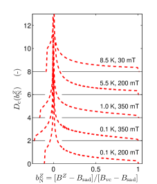
Figure 2: (color online). Component field distributions $D_{\rm c}(b^{Z}_{\rm N})$ computed with the Delrieu’s model assuming $v_{\rm F}=2.0\times 10^{5}$ m/s. Five cases are considered: from top to bottom, in the $B_{\rm c2}(T)$ vicinity at four temperatures, i.e. $T=8.5$, $5.5$, $1.0$ and $0.1$ K, and at low temperature and field but still in the mixed phase, i.e. $T=0.1$ K with $B_{\rm ext}=200$ mT.

We compare $D_{\rm c}(b^{Z}_{\rm N})$ for some selected $(T,B_{\rm ext})$ values computed from the analytical Delrieu’s theory in Fig. 2. We take the material parameter valid for our niobium sample:Maisuradze et al. (2013) $v_{\rm F}=2.0\times 10^{5}$ m/s. We recall that unitless $D_{\rm c}(b^{Z}_{\rm N})$ only depends on $v_{\rm F}$. We recall that $T_{\rm c0}=9.25$ K and $B_{\rm c2}(0)=0.43$ T. As expected and clearly seen in Fig. 2, a distribution is characterized by three fields: its minimum field $B_{\rm min}$, a saddle point field $B_{\rm sad}$ in the field map for which $D_{\rm c}(b^{Z}_{\rm N})$ displays a maximum, and $B_{\rm vc}$ which is the field in the center of a vortex core, i.e. the maximum field in $D_{\rm c}(b^{Z}_{\rm N})$. Note that two features of a distribution are strongly dependent on the $(T,B_{\rm ext})$ values: the shape of the high-field tail and the distance between $B_{\rm min}$ and $B_{\rm sad}$. As shown previously,Maisuradze et al. (2013) the observation of a linear high-field tail for large $B_{\rm ext}$ and low $T$ — clearly seen for the fourth distribution from the top — is a signature in those experimental conditions of the pronounced conical shape of the field variation around the vortex cores. This results from the partial Cooper pair diffraction on the vortex cores. We find it convenient to measure the distance between $B_{\rm min}$ and $B_{\rm sad}$ with the following unitless normalized ratio:

$$\delta B^{\rm n}_{\rm sad,min}=-{B_{\rm min}-B_{\rm sad}\over B_{\rm vc}-B_{\rm sad}}.$$ (12)

The first three distributions from the top of Fig. 2 concern $D_{\rm c}(b^{Z}_{\rm N})$ with $B_{\rm ext}$ in the $B_{\rm c2}(T)$ vicinity. A $\delta B^{\rm n}_{\rm sad,min}$ minimum is predicted around $T=5.5$ K. This should easily be observed experimentally. Although, because of the Gaussian smearing discussed in the next section (Sec. III), $\delta B^{\rm n}_{\rm sad,min}$ is not expected to be as small as predicted. We postpone the discussion of its physical meaning to Sect. V. A close look at the last two $D_{\rm c}(b^{Z}_{\rm N})$ from the top of Fig. 2 illustrates the effect of the field intensity at low temperature. An exotic $D_{\rm c}(b^{Z}_{\rm N})$ is only predicted for a sufficiently large $B_{\rm ext}$.

III Experimental

Here the sample is described, as well as the experimental conditions and the data analysis.

The TF-$\mu$SR measurements reported here have been performed on the single crystal described in Ref. Maisuradze et al., 2013. The small $B_{\rm c2}=430\,(2)$ mT testifies of its high quality and purity, as well as the lack of difference between the distributions measured with the zero-field-cooled or field-cooled procedures at 1.5 K under $B_{\rm ext}=360$ mT.

The new TF-$\mu$SR measurements described here have again been performed at the Swiss Muon Source (S$\mu$S), Paul Scherrer Institute (PSI), Switzerland, using the general purpose spectrometer (GPS) and Dolly spectrometers for $T\geq 1.6$ K. Measurements for $T<1.6$ K have been conducted on the low temperature facility (LTF) spectrometer.

Our niobium sample is a single crystal disk of 13 mm diameter and 2 mm thickness with a three-fold axis oriented normal to the disk. In Fig. 3

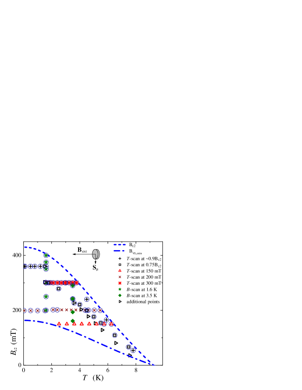
Figure 3: (color online). Temperatures and fields at which measurements have been performed on the niobium single crystal. The geometry for a measurement is depicted by the pictogram: the directions of ${\bf B}_{\rm ext}\parallel\langle 111\rangle$ and of the initial muon beam polarization ${\bf S}_{\mu}$ are given. The $B_{\rm VL,min}(T)$ and $B_{\rm c2}(T)$ lines have been determined as explained in the main text. The points at which the form factor from Delrieu provides a proper description of the experimental $\mu$SR data are encircled.

we specify the values of the temperatures and fields for which measurements have been done. Five temperature scans have been performed at $B_{\rm ext}=$ 300, 200 and 150 mT, and at $0.75B_{\rm c2}$ and $\sim 0.9B_{\rm c2}$. In addition, we report two field scans at 1.6 and 3.5 K. The $B_{\rm c2}(T)$ line has been determined previously.Maisuradze et al. (2013) In addition to the traditional VL and Meissner phases, one needs to consider the intermediate state.Laver et al. (2006) The VL phase is characterized by a single damped oscillation centered around zero as seen for $T=7.3$ and $6.8$ K in Fig. 4.

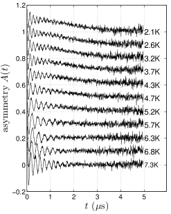
Figure 4: Some asymmetry time spectra for our niobium single crystal with ${\bf B}_{\rm ext}\parallel\langle 111\rangle$ as a function of temperature at $B_{\rm ext}=50$ mT.

The amplitude of the oscillating signal at time $t=0$ is proportional to the fraction of the niobium sample in the VL state. When cooling down to 5.7 K the oscillation is no longer centered around zero and its amplitude is reduced. The signals below 5.7 K represent the sum of an oscillating and Kubo-Toyabe type components. This indicates that the sample has left the mixed phase and part of it is in a zero field condition due to Meissner screening. Performing a few series of measurements as reported in Fig. 4 we have determined the $B_{\rm VL,min}(T)$ line shown in Fig. 3. For $B_{\rm ext}>B_{\rm VL,min}(T)$ the sample is certainly in the mixed phase. We shall use this conservative estimate.

The analysis of the asymmetry time spectra has been done following the method explained in Ref. Maisuradze et al., 2013. Here we would like to stress three points. We do fit the time spectra and not the component field distributions which are only computed for display purpose. Such a distribution is denoted as ${\tilde{D}}^{\rm exp}_{\rm c}(B^{Z})$. The difference between ${\tilde{D}}^{\rm exp}_{\rm c}(B^{Z})$ and ${\tilde{D}}_{\rm c}(B^{Z})$ arises from the contributions of the nuclear ⁹³Nb magnetic moments and the VL disorder to the field distribution at the muon site. These contributions are taken into account in the fits by a single Gaussian function.Brandt (1974) This leads to a Gaussian smearing of ${\tilde{D}}_{\rm c}(B^{Z})$. The influence of disorder is relatively modest in the high-field part of a distribution.Maisuradze et al. (2009) Finally, it has been shown previously that no effect of the muon diffusion on the measured ${\tilde{D}}^{\rm exp}_{\rm c}(B^{Z})$ is expected.Maisuradze et al. (2013)

Data analysis with the Delrieu’s model is exceedingly time consuming. The computation of ${\tilde{D}}_{\rm c}(B^{Z})$ may take few minutes. Since a large number of iterations are needed for fitting a single asymmetry spectrum, an analysis would take many hours. In order to accelerate the analysis we have first computed ${B}^{Z}_{{\bf K}_{m,h}}(\tilde{b}_{i},\tilde{c}_{j})$ setting $\tilde{a}=1$ since it is only a multiplicative factor. We have taken $-30\leq m\leq 30$ and $-30\leq h\leq 30$ and a discrete set of $\tilde{b}_{i}$ and $\tilde{c}_{j}$ parameters, i.e. $\tilde{b}_{i}=10^{n_{i}}$ and $\tilde{c}_{j}=10^{n_{j}}$, with $n_{\alpha}=-3+0.05\times(\alpha-1)$ ($\alpha$ stands for $i$ or $j$). The indicies $i=1,\,2,\,...,\,81$ and $j=1,\,2,\,...,\,101$ correspond to $0.001\leq\tilde{b}\leq 10$ and $0.001\leq\tilde{c}\leq 100$. Because ${B}^{Z}_{{\bf K}_{m,h}}$ is a continuous function of its variables, in the fitting procedure the actual values of ${B}^{Z}_{{\bf K}_{m,h}}(\tilde{a},\tilde{b},\tilde{c})$ were evaluated by interpolation from the precalculated values of $\tilde{a}\times{B}^{Z}_{{\bf K}_{m,h}}(\tilde{b}_{i},\tilde{c}_{j})$ (four-dimensional matrix). A quadratic interpolation has been used to avoid zero second order derivatives during the $\chi^{2}$ minimization. With this method an evaluation of asymmetry time spectrum or ${\tilde{D}}_{\rm c}(B^{Z})$ can be performed within a fraction of second.

IV Typical measured field distributions

In this section typical measured field distributions $D^{\rm exp}_{\rm c}(b^{Z}_{\rm N})$ are displayed. The curves result from a combined fit of the measured asymmetry time spectra to the Delrieu’s theory with $v_{\rm F}$ as a global fitting parameter. The parameters extracted from it are discussed in the next section (Sec. V).

We start by considering the $0.75B_{\rm c2}(T)$ temperature scan. As seen from Fig. 3, it probes the VL from near $T_{\rm c0}$ down to low temperature, i.e. from 7.5 to 1.77 K. Figure 5

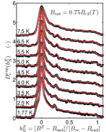
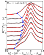
Figure 5: (color online). Some $D_{\rm c}^{\rm exp}(b^{Z}_{\rm N})$ distributions as a function of temperature for $B_{\rm ext}=0.75B_{\rm c2}(T)$. The data and curves have been shifted vertically for better visualization. For each $D_{\rm c}^{\rm exp}(b^{Z}_{\rm N})$ the weak intensity peak for $b^{Z}_{\rm N}$ slightly larger than $0.2$ arises from the contribution of the background — sample holder and cryostat walls — to the distribution. The right panel focuses on the low field regime. The solid lines result from fits to the Delrieu’s theory as described in Sect. II. The dashed line links the $B_{\rm min}$ values.

illustrates some $D^{\rm exp}_{\rm c}(b^{Z}_{\rm N})$. The Delrieu’s theory provides a good description. This is notified in Fig. 3 by encircling the symbols which specify the temperatures and fields of the scan. The determination of $B_{\rm min}$ at high temperature is not very precise due to Gaussian smearing. However, from Fig. 5 it is quite clear that $\delta B^{\rm n}_{\rm sad,min}$ is minimum around $5.0-5.5$ K.

Some $D^{\rm exp}_{\rm c}(b^{Z}_{\rm N})$ from the field

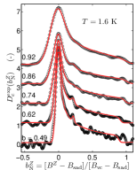
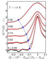
Figure 6: (color online). A selection of $D_{\rm c}^{\rm exp}(b^{Z}_{\rm N})$ distributions as a function of the reduced field $b=B_{\rm ext}/B_{\rm c2}(1.6~{}{\rm K})$. The data and curves have been shifted vertically for better visualization. For each $D_{\rm c}^{\rm exp}(b^{Z}_{\rm N})$ the weak intensity peak for $b^{Z}_{\rm N}\simeq 0.2$ arises from the contribution of the background — sample holder and cryostat walls — to the distribution. The limited statistic for the $b=0.49$ distribution explains its rather noisy nature. The right panel focuses on the low field regime. The solid lines result from fits to the Delrieu’s theory as described in Sect. II. The dashed line links the $B_{\rm min}$ values.

scan at 1.6 K are shown in Fig. 6. Here a smooth $\delta B^{\rm n}_{\rm sad,min}$ increase is observed as $B_{\rm c2}$ is approached. Again, Delrieu provides a good description.

Two $D^{\rm exp}_{\rm c}(b^{Z}_{\rm N})$ are displayed in Fig. 7 for $T\simeq 6.5$ K.

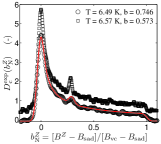
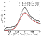
Figure 7: (color online). Two $D_{\rm c}^{\rm exp}(b^{Z}_{\rm N})$ distributions for $T\simeq 6.5$ K at two different fields. The data and curves have been shifted vertically for better visualization. The peaks around $b^{Z}_{\rm N}\simeq 0.3$ arise from the contributions of the background — sample holder and cryostat walls — to the distributions. The right panel focuses on the low field regime. The value of the reduced field $b=B_{\rm ext}/B_{\rm c2}(1.6~{}{\rm K})$ is indicated for each $D_{\rm c}^{\rm exp}(b^{Z}_{\rm N})$. A larger contribution of the VL disorder to the higher field distribution is seen by the reduction of the probability at $B_{\rm sad}$. The solid lines result from fits to the Delrieu’s theory as described in Sect. II for $T=6.49$ K and $b=0.746$. That theory does not fit the data for $T=6.57$ K and $b=0.573$.

The remarkable feature here is that $\delta B^{\rm n}_{\rm sad,min}$ is about the same for the two distributions although the reduced field $b$ is clearly different. This is in contrast to the two previous sets of distributions for which $\delta B^{\rm n}_{\rm sad,min}$ is changing as a function of field or temperature. The Delrieu’s model is unable to account for the data at the lowest $B_{\rm ext}$ value.

V Characteristics of the mixed phase of niobium

Here the physical properties of niobium and its VL deduced from our measured $\mu$SR data are discussed. We shall first consider the parameters extracted from the global fit of the asymmetry time spectra with the Delrieu’s approximation for the form factor. The validity regime of the approximation will be determined. Then the properties of the three characteristic fields of the VL will be analyzed with the numerical solution of the Eilenberger’s theory. Finally, combining our experimental results and the Eilenberger’s theory, the field map of the VL will be established.

V.1 VL parameters and region of validity of the Delrieu’s approximation

We have recorded TF-$\mu$SR asymmetry time spectra for the VL of niobium for a large range of $(T,B_{\rm ext})$ values. From a global fit of the spectra with the Delrieu’s approximation for the form factor we deduce $v_{\rm F}=2.0\,(2)\times 10^{5}$ m/s, in agreement with our previous estimate.Maisuradze et al. (2013) From the measured $\tilde{a}$ and $\tilde{c}$ parameters and Eq. 3 the condensation energy $E_{\rm c}=N_{0}\Delta_{0}^{2}$ is determined. As an example, in Fig. 8

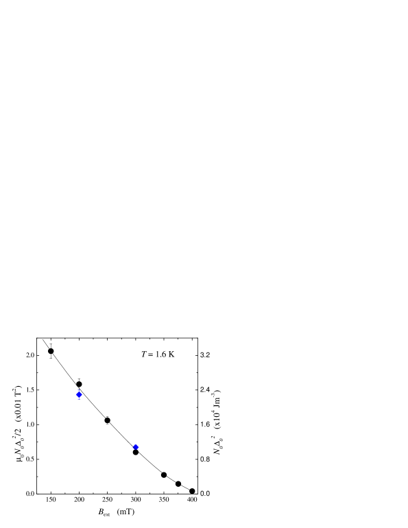
Figure 8: (Color online) Condensation energy $E_{\rm c}=N_{0}\Delta_{0}^{2}$ and $\mu_{0}N_{0}\Delta_{0}^{2}/2$ as a function of $B_{\rm ext}$. The values extracted from the field scan at $1.6$ K are represented as bullets, while diamonds correspond to the two temperature scans at $200$ and $300$ mT. The solid line is a guide to the eyes.

we show the field dependence of $E_{\rm c}=-2\overline{B^{Z}}\tilde{a}/\mu_{0}\tilde{c}$ at $T=1.6$ K. The linear field dependence of $\Delta^{2}_{0}$ given by Eq. 5 is found to be a reasonable approximation. This is again consistent with the results of our analysis of spectra previously taken in the $B_{\rm c2}(T)$ vicinity.

From the analysis of a asymmetry time spectrum recorded near $T_{\rm c0}$ with the GL’s theory we recall that $\kappa_{\rm GL}=0.89\,(1)$.Maisuradze and Yaouanc (2013)

From a close look at Fig. 3 we infer that the Delrieu’s solution for the form factor has a relatively large validity range for niobium, i.e. it is not only valid in the immediate $B_{\rm c2}(T)$ vicinity but also for $0.6\leq T\leq 2.5$ K with $0.2\,{\rm T}\leq B_{\rm ext}<B_{\rm c2}$. The lower temperature bound was previously given.Maisuradze et al. (2013) Since this solution also includes the Abrikosov’s result and it is numerically feasible to use it in a fit procedure, it should be seriously considered for the analysis of TF-$\mu$SR data as a reliable alternative to a pure GL fit for clean s-wave superconductors.Brandt (1997); Yaouanc et al. (1997)

V.2 VL characteristic fields, field distributions and physical origins

Having finished the analysis of the experimental data for various fields and temperatures with the Delrieu’s theory, we now consider those from the Eilenberger’s theory viewpoint. Hence, we can discuss the whole mixed phase, and not only the $B_{\rm c2}(T)$ vicinity. As already mentioned, Klein first calculated the detailed field profiles in the mixed state of niobium by solving the Eilenberger’s equation.Klein (1987) Here based on a numerical algorithm explained in Refs. [Ichioka et al., 1997, 1999a, 1999b; Miranović and Machida, 2003; Nakai et al., 2006], we have calculated $B^{Z}({\bf r})$ within a VL unit cell under periodic boundary conditions for various $B_{\rm ext}$ and $T$ appropriate for the present experimental situations. It will turn out later that $\kappa_{\rm GL}$=1.8 best describes the experimental data, thus all the following computations have been performed using this value. From this information a variety of physical quantities directly related to the present experiments can be deduced, that is, the field distribution ${\tilde{D}}_{\rm c}(B^{Z})$ and therefore the characteristic three field values $B_{\rm min}$, $B_{\rm sad}$, and $B_{\rm vc}$ and their locations within a unit cell.

In order to understand the three possible field patterns, namely as predicted by Ginzburg-Landau (GL), Klein (KL), and Delrieu (DL) which we will identify through the analysis, we first show related field profiles for the three cases in Fig. 9.

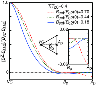
Figure 9: (color online). Results from the Eilenberger’s theory for three field profiles along the vortex-core-$A_{\rm p}$ path, i.e. along $VC-A_{\rm p}$, via $B_{\rm p}$ in the direct space. The ratio value $B_{\rm ext}/B_{\rm c2}(0)=0.18$ corresponds to GL, $B_{\rm ext}/B_{\rm c2}(0)=0.44$ to KL, and $B_{\rm ext}/B_{\rm c2}(0)=0.70$ to DL. We have chosen $T/T_{\rm c0}=0.4$. One of the insert recalls the definition of positions of interest in the unit cell and the other insert magnifies the field profiles between $B_{\rm p}$ and $A_{\rm p}$.

It is seen that

(1) GL field profile for $B_{\rm ext}/B_{\rm c2}(0)=0.18$: $B_{\rm min}$ is located at $B_{\rm p}$ point and $B_{\rm sad}$ at $A_{\rm p}$ in the unit cell. The lowest edge of ${\tilde{D}}_{\rm c}(B^{Z})$ occurs at $B_{\rm p}$.

(2) DL field profile for $B_{\rm ext}/B_{\rm c2}(0)=0.70$: $B_{\rm min}$ is located at $A_{\rm p}$ point while $B_{\rm sad}$ is located at $B_{\rm p}$ point in the unit cell. The lowest edge of ${\tilde{D}}_{\rm c}(B^{Z})$ occurs at $A_{\rm p}$.

(3) KL field profile for $B_{\rm ext}/B_{\rm c2}(0)=0.44$: $A_{\rm p}$ is not saddle any more, but a local minimum. $B_{\rm p}$ is at the absolute minimum where the lowest edge of ${\tilde{D}}_{\rm c}(B^{Z})$ occurs. The saddle points are located in between $A_{\rm p}$ and $B_{\rm p}$. Those features are also seen from Fig. 17 in Ref. Klein, 1987 where the contour plots for the three types of distributions are displayed.

Let us now discuss the physical origins of those three kinds of field profiles. In Fig. 10

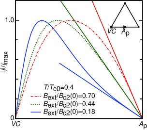
Figure 10: (color online). Three current profiles along the $VC-A_{\rm p}$ path in the direct space. The parameters are the same as in Fig. 9. The currents are normalized to their maximum values. Note the changes of the slope at $A_{\rm p}$ and of the maximum positions for the three profiles.

we show the current profiles around the vortex core along the path from $VC-A_{\rm p}$ where each curve corresponds to that in Fig. 9. In GL ($B_{\rm ext}/B_{\rm c2}(0)=0.18$) the current maximum appears relatively near $VC$ and its amplitude quickly decays towards $A_{\rm p}$. Thus the current curve approaches $A_{\rm p}$ from above to its tangential slope there, implying that the neighboring vortex cores are far apart and the vortex cores are not overlapped. This means that the farthest $B_{\rm p}$ point from the neighboring vortex cores in a unit cell is a $B_{\rm min}$ location. In contrast, the DL case shows that the current maximum moves towards $A_{\rm p}$, with the tangent of the current amplitude being largest among the three profiles. This means that the neighboring vortex cores are densely packed with the vortex cores overlapped, causing $B_{\rm p}$ not to be the minimum field location in a unit cell. The field profile is quite different from that in GL, making $A_{\rm p}$ the minimum field location. In the KL limit those features are in between the GL and DL cases.

Figure 11

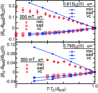
Figure 11: (color online). The three characteristic fields $B_{\alpha}$ ($\alpha=$ minimum, saddle and vortex core) versus the normalized temperature $T/T_{\rm c}(B_{\rm ext})$ for two values of $B_{\rm ext}$. The computed values are shown by filled symbols linked by line segments. We have measured $T_{\rm c}(B_{\rm ext})=5.6$ K and $T_{\rm c}(B_{\rm ext})=3.95$ K for $B_{\rm ext}=200$ and $300$ mT, respectively.

shows the comparison between the theoretical calculations and the experimental data of the $T$-dependence of $B_{\rm min}$, $B_{\rm sad}$ and $B_{\rm vc}$ at two $B_{\rm ext}$ values. The theoretical calculation has been done by varying the $\kappa_{\rm GL}$ value to best fit those three values near $T/T_{\rm c}(B_{\rm ext})=1$. It turns out that the best fitting is achieved for $\kappa_{\rm GL}$=1.8. This value is twice as large as the nominal value $\kappa_{\rm GL}=0.89\,(1)$ of the present sample mentioned before. We notice that the three types of field distributions, namely for the GL, KL and DL cases, are always present irrespective of the choice of $\kappa_{\rm GL}$. It is seen from Fig. 11 that

(1) The initial slopes of the three characteristic fields near $T/T_{\rm c}(B_{\rm ext})=1$ are nicely reproduced for the two $B_{\rm ext}$ values.

(2) Those nice fittings continue to lower temperatures for $B_{\rm min}$ and $B_{\rm sad}$.

(3) In contrast, $B_{\rm vc}$ starts to deviate towards lower temperatures. While the theoretical curves keep increasing linearly with large slopes, the temperature dependence of the experimental data is much weaker.

According to a previous calculation $B_{\rm vc}$ is expected to keep increasing towards zero temperature in the clean limit Miranović and Machida (2003) because of the so-called Kramer-Pesch effect.Pesch and Kramer (1974) As already noticed, a previous NMR experiment by Kung Kung (1970) on vanadium shows the expected linear temperature dependence of $B_{\rm vc}$ in a large temperature range towards zero temperature. Clearly it would be of much interest to perform TF-$\mu$SR measurements on a very clean vanadium sample to confirm Kung’s result, and to extend it to very low temperature.

We show the field dependences of the three characteristic fields in Fig. 12.

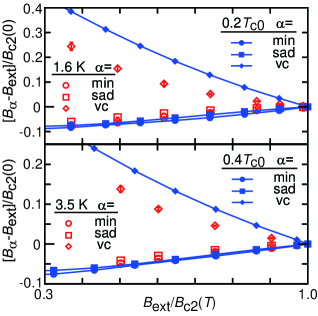
Figure 12: (color online). The three characteristic fields $B_{\alpha}$ ($\alpha=$ minimum, saddle, and vortex core) versus the normalized field $B_{\rm ext}/B_{\rm c2}(T)$ at two temperatures. The computed values are shown by the filled symbols linked by line segments. Experimentally, $B_{\rm c2}=405$ and $321$ mT for $T=1.6$ and $3.5$ K, respectively.

It is seen that the theoretical predictions for $B_{\rm min}$ and $B_{\rm sad}$ follow nicely the experimental results, and the qualitative field dependence of $B_{\rm vc}$ is explained, but quantitatively deviates because in those low temperatures the Kramer-Pesch effect is partially suppressed as mentioned above. Since $B_{\rm vc}$ reflects the spatial structure around a vortex core, the partially suppressed Kramer-Pesch effect implies that the conical shape structure of $B^{Z}({\bf r})$ at the vortex core position is rounded relative to theoretical expectation. However, the linear field tail of the distribution at high field, a signature of the conical feature, is nicely observed at low temperature.Maisuradze et al. (2013)

V.3 VL field map and contour plot

We have previously established the Delrieu’s approximation to be reliable for a large part of the mixed phase.

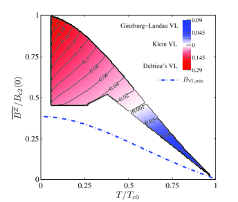
Figure 13: (color online). Contour map of $\delta B^{\rm n}_{\rm sad,min}$ for niobium with ${\bf B}_{\rm ext}\parallel\langle 111\rangle$ computed with the Delrieu’s solution for the form factor. We have restricted the map to the temperature and field regimes properly described by that solution. We specify the regimes consistent with Delrieu, Klein and Ginzburg-Landau. The dashed-dotted line displays $B_{\rm VL,min}(T)$.

The computed $\delta B^{\rm n}_{\rm sad,min}$ map displayed in Fig. 13 visualizes the region of the mixed phase where the approximation is reliable for the analysis of our niobium data. Remarkably, the $(T,B_{\rm ext})$ points close to $B_{\rm c2}$ at which $\delta B^{\rm n}_{\rm sad,min}=0$ effectively correspond in Fig. 5 to the temperature where the measured $\delta B^{\rm n}_{\rm sad,min}$ is minimum. This occurs around $5.5$ K. It is because of the Gaussian smearing that $\delta B^{\rm n}_{\rm sad,min}$ does not vanish experimentally.

From Delrieu, $\delta B^{\rm n}_{\rm sad,min}=0$ at the border between the DL and GL VL region. This border belongs to the Klein’s regime that we discuss now.

In order to examine the diagram obtained experimentally in Fig. 13, we have done extensive computations to construct the corresponding diagram whose results are displayed in Fig. 14. The overall features in Figs. 13 and 14 coincide, namely, DL occupies the higher field region while GL is located at lower field. The KL region is in the middle. However, the KL regime is no longer limited to the border between the DL and GL regions: it has an appreciable extension. This is a key result obtained from the Eilenberger’s solution. The Delrieu’s approximation is too rough to capture the subtilities in $B^{Z}({\bf r})$ in the KL regime; see Fig. 9. In addition, while in the vicinity of $B_{\rm c2}(T)$ the values of $\delta B^{\rm n}_{{\rm sad},{\min}}$ in Figs. 13 and 14 strikingly correspond for a given field and temperature, outside that regime deviations between the results in the two figures are clearly found: a given $\delta B^{\rm n}_{{\rm sad},{\min}}$ value in the DL region is only weakly temperature dependent in Fig. 14, in contrast to the results presented in Fig. 13. Before going further in comparing the experimentally deduced and the theoretical diagram, some comments are in order.

Figure 13 considers $\overline{B^{Z}}$ rather than $B_{\rm ext}$ because it is this parameter which enters into the Delrieu’s theory. However, in pratice $\overline{B^{Z}}\simeq B_{\rm ext}$. Because the lower field border of the measured phase is dependent on the experimental conditions, for the sake of completeness, we have extended the theoretical diagram in Fig. 14 to lower fields and temperatures than in Fig. 13. We stress that while the Delrieu’s formula does not describe the low temperature region of the mixed phase as seen in Fig. 13, the numerical solution of the Eilenberger’s equation is expected to provide a proper description.

The data set shown in Fig. 6 corresponds to scanning the field at a fixed low temperature in Fig. 14.

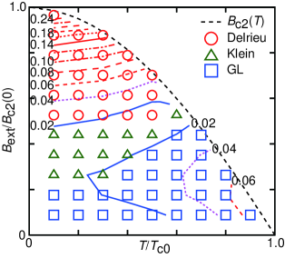
Figure 14: (color online). Contour map of $\delta B^{\rm n}_{\rm sad,min}$ for niobium with ${\bf B}_{\rm ext}\parallel\langle 111\rangle$ computed with the Eilenberger’s equation. In the Klein’s region two minimal field positions exist; see the insert on the right in Fig. 9. The data in Fig. 6 (Fig. 7) correspond to scanning vertically at low (high) temperature. For the data in Fig. 5 scanning is done parallel to the $B_{\rm c2}(T)$ line.

As this map implies, $\delta B^{\rm n}_{\rm sad,min}$ increases as $B_{\rm ext}$ increases. In fact, as seen from Fig. 15

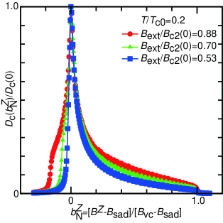
Figure 15: (color online). The normalized field distributions $D_{\rm c}(b^{Z}_{\rm N})/D_{\rm c}(0)$ for three field values at $T/T_{\rm c0}=0.2$ corresponding to the data in the right hand panel of Fig. 6. Those are traversing the map in Fig. 14 vertically.

where we show the computed normalized field distributions $D_{\rm c}(b^{Z}_{\rm N})/D_{\rm c}(0)$ under a fixed temperature ($T/T_{\rm c0}=0.2$) for three field values, as $B_{\rm ext}$ increases, $B_{\rm min}$ moves to the lower field side, i.e. to the left of the field scale. This explains the fact in Fig. 6 that $B_{\rm min}$ increases in absolute value as $B_{\rm ext}$ increases.

As for Fig. 5 where the scanning path is taken parallel to the $B_{\rm c2}(T)$ line, it is seen from Fig. 14 that $\delta B^{\rm n}_{\rm sad,min}$ decreases first and then increases towards lower temperatures, coinciding with the data in Fig. 5.

Finally as for GL, Fig. 7 shows that the two distributions are hardly distinguishable because the two distributions are both inside the GL region in Fig. 14 where the GL distribution is universal and scaled.

Those various scanning data throughout the $B_{\rm ext}-T$ plane demonstrate precise correspondence between Eilenberger’s theory and experiment, supporting the existence of the three distinct characteristic field distributions, i.e. the GL, KL and DL distributions.

VI Summary of the results obtained in this study; possible improvements of the analysis and data recording

In summary, combining TF-$\mu$SR measurements analyzed with the Delrieu’s analytical solution for the form factor — supplemented with conventional phenomenological formulas for the physical parameters — and the numerical solutions of the quasiclassical Eilenberger’s equation to get $B^{Z}({\bf r})$, we have established that the VL of niobium with ${\bf B}_{\rm ext}$ applied along a three-fold axis is characterized by three successive regions as the sample is cooled down from $T_{\rm c0}$. Hence, our work supports the predictions of Abrikosov, Klein, and Delrieu, respectively. It seems that it has never been done previously.

The experimental data, notably the three regions in the mixed phase, are explained by the Eilenberger’s theory taking the Fermi surface cylindrical, but the field and temperature dependences of $B_{\rm vc}$. Disturbing, a $\kappa_{\rm GL}$ parameter twice as large as the measured value has to be assumed. We know of two sources for possible explanations of the discrepancies.

(1) Our numerical solution of the Eilenberger’s equation does not take into account the Fermi velocity anisotropy and gap anisotropy known to exist as seen in the $B_{\rm c2}$ anisotropy.Williamson and Valby (1970); Williamson (1970) In particular the Fermi velocity anisotropy generally increases $B_{\rm c2}$ value, thus causing the estimate of $\kappa_{\rm GL}$ to change.

(2) We are regarding $\kappa_{\rm GL}$ as an effective parameter because the theory assumes the clean limit. Although our sample is extremely clean,Maisuradze et al. (2013) it is known that defects and impurities act to increase $\kappa_{\rm GL}$ from the nominal value.

We have to deal with three sources of field distributions at the muon site: the nuclear ⁹³Nb magnetic moments, the VL itself and the effect of the VL disorder. To a good approximation, the component field distribution from the nuclear moments in a TF-$\mu$SR experiment is Gaussian.Yaouanc and Dalmas de Réotier (2011) We have just discussed how the description of the distribution from the VL itself can be improved. It is known that modeling the effect of the VL disorder with a Gaussian field function as done in this report is a rough approximation. A close look at Fig. 2 of Ref. Maisuradze et al., 2013 shows it definitively, in particular in the vicinity of the low-field tail. In fact, the translational correlations of the vortex cores are neglected in the Gaussian approximation.Yaouanc et al. (2013) To progress we need to recognize that the VL is not a two-dimensional lattice, but a three-dimensional lattice, i.e. we are dealing with the flux-line lattice (FLL). As for any lattice, disorder has to be considered. In the FLL case we need to remember that the collective behaviour matters.Feigel’man et al. (1989) In the absence of dislocations, if disorder is not too strong the FLL is periodic, as clearly demonstrated by SANS measurements, but the FLL translational order decays only algebraically rather than exponentially,Klein et al. (2001); Laver et al. (2008) as expected theoretically.Nattermann (1990) In fact, a so-called Bragg glass state is expected,Giamarchi and Doussal (1995) and observed.Klein et al. (2001); Laver et al. (2008) However, we stress that it was found for samples with appreciable disorder. It is still a challenge to observe it for a clean sample such as ours. A numerical method to account for the Bragg-glass state has been devised for the analysis of SANS measurements.Laver et al. (2008) This has yet to be done for the $\mu$SR counterpart.

Neither the Delrieu’s analytical solution, nor the numerical solution of the Eilenberger’s equation describes the measured distributions below 0.6 K.Maisuradze et al. (2013) A proper account of the vortex-lattice residual disorder may round up the predicted sharp conical field shape at the VL vortex cores and explain the measurements below $0.6$ K.

Up to now we have discussed possible improvements of the data analysis. But the experimental conditions themselves could also be optimized. All the TF-$\mu$SR asymmetry time spectra have been recorded on a single crystal disk with ${\bf B}_{\rm ext}$ parallel to the disk axis; see pictogram in Fig. 3. In this geometry inhomogeneities due to the demagnetization field near the sample boundaries may have to be considered. An improved experimental setup would require ${\bf B}_{\rm ext}$ to be applied perpendicular to the disk axis. However, for the needed high $B_{\rm ext}$ values this is not possible since the positive muon is a charge particle, and as such would be deflected from its trajectory according to the Lorentz force. Hence, ${\bf B}_{\rm ext}$ should be kept into the direction we have chosen. Therefore to improve on the experimental conditions, an elliptical single sample would have to be used.

The form factors of a vortex lattice can be studied by the SANS technique. It is well known that the exact solution of GL theory gives some $K_{m,n}$ form factors of opposite sign relative to those predicted by analytical approximations of GL theory or the London model; See Ref. Brandt, 1997 for a discussion. Regarding Delrieu’s solution, the signs of the form factors are the same as is in the Abrikosov’s solution and are given by the factor $(-1)^{mh}$.Maisuradze and Yaouanc (2013) Only the magnitude of the form factors varies with the values of the parameters $\tilde{b}$ and $\tilde{c}$. The signs of the form factors at high order from the Eilenberger solution have still to be evaluated. This requires to get the solution accurate enough to extract those higher order harmonics because those become extremely small numbers.

VII Conclusions and perspectives

In conclusion, combining the TF-$\mu$SR experimental technique with the Delrieu’s analytical solution and numerical solutions of the quasiclassical Eilenberger’s equation, we have observed the theoretically expected three regions in the mixed phase of niobium with ${\bf B}_{\rm ext}$ applied along a three-fold axis. We do not know of any previous experimental observation of the three regions. Our results should apply to any clean s-wave superconductor with a triangular vortex lattice.

The experimental data have been recorded at high statistics and the analysis has been done with advances methods. Possible improvements of the data analysis and experimental conditions have been pointed out. We hope that our work will motivate people to analyze TF-$\mu$SR asymmetry time spectra for other s-wave superconductors with the framework presented here. An obvious candidate is vanadium, the sample of which should be in the extremely clean limit.

References

- Tinkham (1996) M. Tinkham, Introduction to Superconductivity (McGraw-Hill, New York, 1996).
- Ketterson and Song (1999) J. B. Ketterson and S. N. Song, Superconductivity (Cambridge University Press, Cambridge, 1999).
- Abrikosov (1957) A. A. Abrikosov, Sov. Phys. JETP 5, 1174 (1957).
- Gor’kov (1959) L. P. Gor’kov, Sov. Phys. JETP 9, 1364 (1959).
- Sonier et al. (2000) J. E. Sonier, J. H. Brewer, and R. F. Kiefl, Rev. Mod. Phys. 72, 769 (2000).
- Sonier (2007) J. E. Sonier, Reports Prog. in Phys. 70, 1717 (2007).
- Delrieu (1972) J. M. Delrieu, J. Low Temp. Phys. 6, 197 (1972).
- Eilenberger (1968) G. Eilenberger, Z. Phys. 214, 195 (1968).
- Klein (1987) U. Klein, J. Low Temp. Phys. 69, 1 (1987).
- Kung (1970) A. Kung, Phys. Rev. Lett. 25, 1006 (1970).
- Dalmas de Réotier and Yaouanc (1997) P. Dalmas de Réotier and A. Yaouanc, J. Phys.: Condens. Matter 9, 9113 (1997).
- Yaouanc and Dalmas de Réotier (2011) A. Yaouanc and P. Dalmas de Réotier, Muon Spin Rotation, Relaxation, and Resonance: Applications to Condensed Matter, International Series of Monographs on Physiscs 147 (Oxford University Press, Oxford, 2011).
- Maisuradze et al. (2013) A. Maisuradze, A. Yaouanc, R. Khasanov, A. Amato, C. Baines, D. Herlach, R. Henes, P. Keppler, and H. Keller, Phys. Rev. B 88, 140509 (2013).
- Schelten et al. (1971) J. Schelten, H. Ullmaier, and W. Schmatz, Phys. Status Solidi B 48, 619 (1971).
- Kahn and Parette (1973) R. Kahn and G. Parette, Solid State Commun. 13, 1839 (1973).
- Forgan et al. (2002) E. M. Forgan, S. J. Levett, P. G. Kealey, R. Cubitt, C. D. Dewhurst, and D. Fort, Phys. Rev. Lett. 88, 167003 (2002).
- Mühlbauer et al. (2009) S. Mühlbauer, C. Pfleiderer, P. Böni, M. Laver, E. M. Forgan, D. Fort, U. Keiderling, and G. Behr, Phys. Rev. Lett. 102, 136408 (2009).
- Herlach et al. (1990) D. Herlach, G. Majer, J. Major, J. Rosenkranz, M. Schmolz, W. Schwarz, A. Seeger, W. Templ, E. H. Brandt, U. Essmann, K. Fürderer, and M. Gladisch, Hyperfine Interactions 63, 41 (1990).
- Werthamer (1969) N. R. Werthamer, in Superconductivity, Vol. 1, edited by R. D. Parks (Marcel Dekker, New York, 1969).
- Maisuradze and Yaouanc (2013) A. Maisuradze and A. Yaouanc, Phys. Rev. B 87, 134508 (2013).
- Adachi et al. (2011) H. M. Adachi, M. Ishikawa, T. Hirano, M. Ichioka, and K. Machida, J. Phys. Soc. Jpn. 80, 113702 (2011).
- Brandt (1997) E. H. Brandt, Phys. Rev. Lett. 78, 2208 (1997).
- Miranović and Machida (2003) P. Miranović and K. Machida, Phys. Rev. B 67, 092506 (2003).
- Laver et al. (2006) M. Laver, E. M. Forgan, S. P. Brown, D. Charalambous, D. Fort, C. Bowell, S. Ramos, R. J. Lycett, D. K. Christen, J. Kohlbrecher, C. D. Dewhurst, and R. Cubitt, Phys. Rev. Lett. 96, 167002 (2006).
- Brandt (1974) E. H. Brandt, Phys. Stat. Sol. B 65, 469 (1974).
- Maisuradze et al. (2009) A. Maisuradze, R. Khasanov, A. Shengelaya, and H. Keller, J. Phys.: Condens. Matter 21, 075701 (2009).
- Yaouanc et al. (1997) A. Yaouanc, P. Dalmas de Réotier, and E. H. Brandt, Phys. Rev. B 55, 11107 (1997).
- Ichioka et al. (1997) M. Ichioka, N. Hayashi, and K. Machida, Phys. Rev. B 55, 6565 (1997).
- Ichioka et al. (1999a) M. Ichioka, A. Hasegawa, and K. Machida, Phys. Rev. B 59, 8902 (1999a).
- Ichioka et al. (1999b) M. Ichioka, A. Hasegawa, and K. Machida, Phys. Rev. B 59, 184 (1999b).
- Nakai et al. (2006) N. Nakai, P. Miranović, M. Ichioka, and K. Machida, Phys. Rev. B 73, 172501 (2006).
- Pesch and Kramer (1974) W. Pesch and L. Kramer, J. Low Temp. Phys. 15, 367 (1974).
- Williamson and Valby (1970) S. J. Williamson and L. E. Valby, Phys. Rev. Lett. 24, 1061 (1970).
- Williamson (1970) S. J. Williamson, Phys. Rev. B 2, 3545 (1970).
- Yaouanc et al. (2013) A. Yaouanc, A. Maisuradze, and P. Dalmas de Réotier, Phys. Rev. B 87, 134405 (2013).
- Feigel’man et al. (1989) M. V. Feigel’man, V. B. Geshkenbein, A. I. Larkin, and V. M. Vinokur, Phys. Rev. Lett. 63, 2303 (1989).
- Klein et al. (2001) T. Klein, I. Joumard, S. Blanchard, J. Marcus, R. Cubitt, T. Giamarchi, and P. L. Doussal, Nature 413, 404 (2001).
- Laver et al. (2008) M. Laver, E. M. Forgan, A. B. Abrahansen, C. Bowell, T. Geue, and R. Cubitt, Phys. Rev. Lett. 100, 107001 (2008).
- Nattermann (1990) T. Nattermann, Phys. Rev. Lett. 64, 2454 (1990).
- Giamarchi and Doussal (1995) T. Giamarchi and P. L. Doussal, Phys. Rev. B 52, 1242 (1995).