Advanced Finite-Temperature Lanczos Method for anisotropic spin systems

Abstract

It is virtually impossible to evaluate the magnetic properties of large anisotropic magnetic molecules numerically exactly due to the huge Hilbert space dimensions as well as due to the absence of symmetries. Here we propose to advance the Finite-Temperature Lanczos Method (FTLM) to the case of single-ion anisotropy. The main obstacle, namely the loss of the spin rotational symmetry about the field axis, can be overcome by choosing symmetry related random vectors for the approximate evaluation of the partition function. We demonstrate that now thermodynamic functions for anisotropic magnetic molecules of unprecedented size can be evaluated.

I Introduction

The magnetism of anisotropic spin systems in particular magnetic molecules is very rich and leads to interesting phenomena such as bistability and quantum tunneling, both related to the anisotropy barrier Gatteschi et al. (2006). Nevertheless many Single Molecule Magnets (SMM) such as Mn₁₂ acetate Lis (1980); Sessoli et al. (1993a, b); Thomas et al. (1996); Gomes et al. (1998); Cornia et al. (2001); Gatteschi and Sessoli (2003) constitute a massive challenge for theoretical investigations since the underlying Hilbert space of the molecular many-spin system is orders of magnitude too big for an exact and complete matrix diagonalization. In cases such as that of Mn₁₂ the lowest zero-field split multiplet is largely separated from the rest of the energy spectrum so that it can approximately be treated as a single giant spin for low-enough temperatures.

For molecules where such a separation is impossible one would like the investigate the full spectrum in order to understand their magnetic properties. The largest species where such a procedure was possible are the Mn${}_{6}^{\text{III}}$ of Euan Brechin’s group Milios et al. (2007); Carretta et al. (2008) as well as the Mn${}_{6}^{\text{III}}$M molecules of Thorsten Glaser’s group Glaser et al. (2009); Glaser (2011); Hoeke et al. (2012a, b, 2013, 2014). The numerically most demanding member of the latter family, Mn${}_{6}^{\text{III}}$Cr${}^{\text{III}}$, possesses a Hilbert space dimension of 62.500, which thanks to inversion symmetry can be reduced to half the size. Nevertheless, a single calculation for one external magnetic field value including a powder average over 25 directions needs about a week on an 8 core workstation, not to mention the necessary 46 GB of RAM. Exact calculations for larger magnetic molecules are thus virtually impossible. It would therefore be very appealing to have a reliable approximation at one’s disposal.

In the realm of spin systems that are described by the Heisenberg model the Finite-Temperature Lanczos Method (FTLM) Jaklic and Prelovsek (1994, 2000); Manthe and Huarte-Larranaga (2001); Long et al. (2003); Aichhorn et al. (2003), which is a so-called trace estimator, was successfully applied to temperature and field dependent magnetic observables for lattice systems Shannon et al. (2004); Zerec et al. (2006); Schmidt et al. (2007); Siahatgar et al. (2012), to optical conductivities Jaklič and Prelovšek (1994) and a variety of molecules Schnack and Wendland (2010); Schnack and Heesing (2013) up to very large Hilbert spaces with dimensions of the order of $10^{10}$ Zheng et al. (2013). Although the underlying Lanczos method Lanczos (1950) is not restricted to isotropic spin models and has also been used to determine low-lying eigenstates of Mn₁₂ acetate Regnault et al. (2002); Chaboussant et al. (2004), the accuracy of FTLM largely increases if symmetries of the Hamiltonian can be exploited. In anisotropic spin systems the spin-rotational, i.e. SU(2) symmetry or even the simpler $\!\hbox{}\mathop{\vphantom{S}\smash{S}}\limits_{\sim}\!{}^{z}$-symmetry are lost. Therefore, a straight forward extension of FTLM appears doubtful.

In this article we demonstrate that by restoring time-reversal invariance in the set of initial random vectors used for FTLM the accuracy of magnetic observables can be drastically improved compared to a naive ansatz. Interestingly, this mainly concerns high-temperature quantities such as $\chi T$ vs. $T$ or $\mu_{\text{eff}}$ vs. $T$, which without restoring symmetry tend to systematically deviate from the correct result, i.e. the paramagnetic limit. We show with a few examples that FTLM yields results that are virtually indistinguishable from the exact ones and that one can now treat systems of unprecedented size, which is exemplarily demonstrated for a fictitious Mn${}_{12}^{\text{III}}$ molecule.

The article is organized as follows. In Section II basics of the Finite-Temperature Lanczos method are repeated. Section III discusses the problem of reduced symmetries. Section IV discusses the performance of the method for large molecules. The article closes with summary and outlook.

II Recapitulation of the Finite-Temperature Lanczos Method

The exact partition function $Z$ depending on temperature $T$ and magnetic field $B$ is given by a trace

$$Z(T,B) = \sum_{\nu}\;\langle\,{\nu}\,|\,e^{-\beta\!\hbox{}\mathop{\vphantom{H}\smash{H}}\limits_{\sim}\hbox{}\!}\,|\,{\nu}\,\rangle\ ,$$ (1)

where $\{\,|\,{\nu}\,\rangle\}$ denotes an orthonormal basis of the respective Hilbert space. Following the ideas of Refs. Jaklic and Prelovsek (1994, 2000) the unknown matrix elements are approximated as

$$\langle\,{\nu}\,|\,e^{-\beta\!\hbox{}\mathop{\vphantom{H}\smash{H}}\limits_{\sim}\hbox{}\!}\,|\,{\nu}\,\rangle \approx \sum_{n=1}^{N_{L}}\;\langle\,{\nu}\,|\,{n(\nu)}\,\rangle e^{-\beta\epsilon_{n}^{(\nu)}}\langle\,{n(\nu)}\,|\,{\nu}\,\rangle\ .$$ (2)

For the evaluation of the right hand side of Eq. (2) $\,|\,{\nu}\,\rangle$ is taken as the initial vector of a Lanczos iteration of $N_{L}$ steps, which generates a respective Krylov space. As common for the Lanczos method the Hamiltonian is diagonalized in this Krylow space, which yields the $N_{L}$ Lanczos eigenvectors $\,|\,{n(\nu)}\,\rangle$ as well as the associated Lanczos energies $\epsilon_{n}^{(\nu)}$, where $n=1,\dots,N_{L}$. The notation $n(\nu)$ reminds one that the $\,|\,{n(\nu)}\,\rangle$ belong to the Krylov space derived from the original state $\,|\,{\nu}\,\rangle$.

The parameter $N_{L}$ needs to be large enough to reach the extremal energy eigenvalues but should not be too large in order not to run into problems of numerical accuracy. $N_{L}\approx 100$ is a typical and good value.

In addition, the complete and thus very large sum over all states $\,|\,{\nu}\,\rangle$ is replaced by a summation over a set of $R$ random vectors. The partition function is thus approximated by

$$Z(T,B) \approx \frac{\text{dim}({\mathcal{H}})}{R}\sum_{\nu=1}^{R}\;\sum_{n=1}^{N_{L}}\;e^{-\beta\epsilon_{n}^{(\nu)}}|\langle\,{n(\nu)}\,|\,{\nu}\,\rangle|^{2}\ .$$ (3)

Symmetries can be taken into account by applying the procedure for every orthogonal subspace ${\mathcal{H}}(\Gamma)$, i.e.

$$Z(T,B) \approx \sum_{\Gamma}\;\frac{\text{dim}({\mathcal{H}}(\Gamma))}{R_{\Gamma}}\sum_{\nu=1}^{R_{\Gamma}}\;\sum_{n=1}^{N_{L}}\;$$ (4)

$$\times e^{-\beta\epsilon_{n}^{(\nu,\Gamma)}}|\langle\,{n(\nu,\Gamma)}\,|\,{\nu,\Gamma}\,\rangle|^{2}\ .$$

$\Gamma$ denotes the irreducible representations of the symmetry group. Observables are then evaluated as

$$O(T,B) \approx \frac{1}{Z(T,B)}\sum_{\Gamma}\;\frac{\text{dim}({\mathcal{H}}(\Gamma))}{R_{\Gamma}}\sum_{\nu=1}^{R_{\Gamma}}\;\sum_{n=1}^{N_{L}}\;e^{-\beta\epsilon_{n}^{(\nu,\Gamma)}}$$ (5)

$$\times\langle\,{n(\nu,\Gamma)}\,|\,\!\hbox{}\mathop{\vphantom{O}\smash{O}}\limits_{\sim}\hbox{}\!\,|\,{\nu,\Gamma}\,\rangle\langle\,{\nu,\Gamma}\,|\,{n(\nu,\Gamma)}\,\rangle\ .$$

The very positive experience is that even for large problems the number of random starting vectors as well as the number of Lanczos steps can be chosen rather small, e.g. $R\approx 100,N_{L}\approx 100$ Schnack and Wendland (2010); Schnack and Heesing (2013). Since Lanczos iterations consist of matrix vector multiplications they can be parallelized by penMP directives. In ur programs this is further accelerated by an analytical state coding and an evaluation of matrix elements of the Hamiltonian “on the fly” Schnack et al. (2008).

III The problem of anisotropic spin systems

For the anisotropic spin systems considered in this publication the complete Hamiltonian of the spin system is given by the Heisenberg term, the single-ion anisotropy, and the Zeeman term, i. e.

$$\!\hbox{}\mathop{\vphantom{H}\smash{H}}\limits_{\sim}\hbox{}\! = -2\;\sum_{i<j}\;{J}_{ij}\!\hbox{}\mathop{\vphantom{\vec{s}}\smash{\vec{s}}}\limits_{\sim}\!{}_{i}\cdot\!\hbox{}\mathop{\vphantom{\vec{s}}\smash{\vec{s}}}\limits_{\sim}\!{}_{j}+\sum_{i}\;\!\hbox{}\mathop{\vphantom{\vec{s}}\smash{\vec{s}}}\limits_{\sim}\!{}_{i}\cdot{\mathbf{D}}_{i}\cdot\!\hbox{}\mathop{\vphantom{\vec{s}}\smash{\vec{s}}}\limits_{\sim}\!{}_{i}$$

$$+\mu_{B}\,B\,\sum_{i}\;g_{i}\!\hbox{}\mathop{\vphantom{s}\smash{s}}\limits_{\sim}\!{}^{z}_{i}\ .$$

${J}_{ij}$ is the exchange parameter between spins at sites $i$ and $j$. A negative ${J}_{ij}$ corresponds to an antiferromagnetic interaction, a positive one to a ferromagnetic interaction. For the sake of simplicity it is assumed that the $g_{i}$ are numbers. ${\mathbf{D}}_{i}$ denotes the single-ion anisotropy tensor, which in its eigensystem $\vec{e}_{i}^{\,1}$, $\vec{e}_{i}^{\,2}$, $\vec{e}_{i}^{\,3}$, can be decomposed as

$${\mathbf{D}}_{i} = D_{i}\vec{e}_{i}^{\,3}\otimes\vec{e}_{i}^{\,3}+E_{i}\left\{\vec{e}_{i}^{\,1}\otimes\vec{e}_{i}^{\,1}-\vec{e}_{i}^{\,2}\otimes\vec{e}_{i}^{\,2}\right\}\ .$$ (7)

The magnetization can be derived from the thermodynamic potential $G(T,\vec{B})$

$$\vec{{\mathcal{M}}}(T,\vec{B}) = -\frac{\partial\,{}}{\partial\,{\vec{B}}}\;\,G(T,\vec{B})$$ (8)

$$G(T,\vec{B}) = -k_{B}T\ \text{ln}\left[Z(T,\vec{B})\right]\ .$$ (9)

In the following we consider only the spatial component of $\vec{{\mathcal{M}}}$ that is parallel to the field direction. To avoid the very costly evaluation of eigenvectors we approximate the derivative in (8), equivalently the evaluation of the magnetization according to (5), by a difference quotient.

The major problem of a straight forward application of FTLM is the general loss of symmetries, and in view of the magnetization the loss of the $\!\hbox{}\mathop{\vphantom{S}\smash{S}}\limits_{\sim}\!{}^{z}$-symmetry. To understand this aspect better we would like to repeat the benefits of an $\!\hbox{}\mathop{\vphantom{S}\smash{S}}\limits_{\sim}\!{}^{z}$-symmetry. This symmetry means that the complete Hilbert space can be decomposed into mutually orthogonal subspaces ${\mathcal{H}}(M)$ for each total magnetic quantum number $M$. For each energy eigenvalue in ${\mathcal{H}}(M)$ there exists a degenerate eigenvalue in ${\mathcal{H}}(-M)$. Therefore, with a Lanczos procedure one would only generate the approximate levels for non-negative $M$ and take those for negative $M$ as copies, which automatically preserves the $\!\hbox{}\mathop{\vphantom{S}\smash{S}}\limits_{\sim}\!{}^{z}$-symmetry in the pseudo spectrum. In terms of the magnetization this guarantees the very general symmetry

$$\vec{{\mathcal{M}}}(T,-\vec{B}) = -\vec{{\mathcal{M}}}(T,\vec{B})\ .$$ (10)

It is also related to the properties of magnetic observables at high temperatures since these rely on trace formulas such as

$$\mbox{Tr}\left(\!\hbox{}\mathop{\vphantom{S}\smash{S}}\limits_{\sim}\!{}^{z}\right) = 0\ ,$$ (11)

as can be seen in high-temperature expansions Schmidt et al. (2001); Thuesen et al. (2010); Schmidt et al. (2011); Lohmann et al. (2014). If a relation such as (11) is violated in an approximation the high-temperature limit of the magnetization (or susceptibility) does not correspond to the correct paramagnetic limit.

In an approximation which rests on random states, as FTLM does, a symmetry that is broken by every random vector, is only restored in the limit of very large sets of random realizations (central limit theorem). A scheme such as outlined above, where one duplicates every Lanczos energy eigenvalue for the subspace with negative magnetic quantum number, restores the $\!\hbox{}\mathop{\vphantom{S}\smash{S}}\limits_{\sim}\!{}^{z}$-symmetry even for small numbers of random vectors. For anisotropic spin systems such a scheme is not applicable, because the simple $\!\hbox{}\mathop{\vphantom{S}\smash{S}}\limits_{\sim}\!{}^{z}$-symmetry does no longer apply. But the very general symmetry (10), that goes back to time reversal invariance of Hamiltonian (III) when the magnetic field is inverted simultaneously, still applies. It means, that every Lanczos energy eigenvector that is evaluated for a certain field $\vec{B}$ has a time-symmetric counterpart that is the respective eigenvector for $-\vec{B}$. Taking $\vec{B}$ as the quantization direction, i.e. $\vec{B}=B\vec{e}_{z}$, this yields for a Lanczos energy eigenvector

$$\,|\,{n(\nu)}\,\rangle = \sum_{\vec{m}}\,c_{\vec{m}}\,|\,{\vec{m}}\,\rangle$$ (12)

the following vector as symmetry-related counterpart

$$\,|\,{\tilde{n}(\nu)}\,\rangle = \sum_{\vec{m}}\,c_{\vec{m}}^{*}\,|\,{-\vec{m}}\,\rangle\ .$$ (13)

Here $\,|\,{\vec{m}}\,\rangle$ is a state of the product basis (where each single-spin state is an eigenstate of the single $\!\hbox{}\mathop{\vphantom{s}\smash{s}}\limits_{\sim}\!{}_{i}^{z}$ operator), while $\,|\,{-\vec{m}}\,\rangle$ denotes the basis state, where all single magnetic quantum numbers $m_{i}$ are inverted compared to $\,|\,{\vec{m}}\,\rangle$. The coefficients $c_{\vec{m}}^{*}$ are complex conjugated with respect to $c_{\vec{m}}$. It is very important to note, that the two states are not degenerate. $\,|\,{n(\nu)}\,\rangle$ is an eigenstate of (III) for $B$ with magnetization ${\mathcal{M}}_{n}=\langle\,{n(\nu)}\,|\,\mu_{B}\sum_{i}g_{i}\!\hbox{}\mathop{\vphantom{s}\smash{s}}\limits_{\sim}\!{}^{z}_{i}\,|\,{n(\nu)}\,\rangle$, whereas $\,|\,{\tilde{n}(\nu)}\,\rangle$ is an eigenstate for $-B$, but then indeed with the same energy and opposite magnetization, i.e. $-{\mathcal{M}}_{n}$.

It turns out that the application of such a procedure would be very costly, since all eigenstates (12) would be needed in order to construct the symmetry-related states (13), for which the energy expectation value (at negative $B$) would have to be evaluated. We therefore propose the following simplification. For every random starting vector $\,|\,{\nu}\,\rangle$ of our Lanczos procedure we also take its symmetry-related counterpart as a random starting vector. This does not exactly guarantee (11), but comes close to a rather high precision.

IV Application to large spin systems

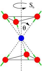
Figure 1: Structure of the S₆-symmetric molecules M1 and M2 investigated in this section, compare also Ref. Glaser (2011). M1: 6 spins in two triangles without central spin; M2: like M1 but with seventh, central spin. The thick short bars denote easy axes.

In the following we demonstrate the potential of the method. In the first part we choose model systems that can also be treated exactly since this allows to estimate the numerical accuracy qualitatively without having to care about experimental uncertainties or inappropriate parameters of the model. Model system M1 is inspired by Mn${}_{6}^{\text{III}}$ molecules Glaser et al. (2010) with 6 spins $s=2$ arranged in two uncoupled equilateral triangles. We choose a fictitious nearest neighbor exchange interaction $J=\pm 0.314$ cm^-1 and single-ion anisotropy tensors with $D_{i}=-5.0$ cm^-1, $E_{i}=0$ and an angle of $\Theta=40^{\circ}$ of the local easy axis to the S₆-symmetry axis of the molecule. The polar angles differ by $\Delta\phi=120^{\circ}$ between neighbors according to the S₆-symmetry, compare Fig. 1 without central ion.

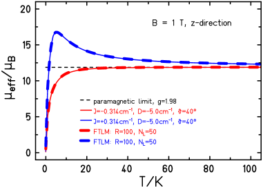
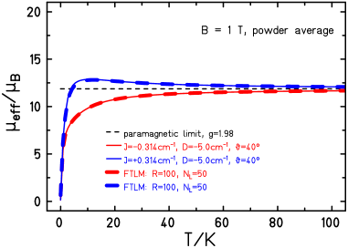
Figure 2: Effective magnetic moment of model system M1: moment along $z$-direction (top), powder averaged moment (bottom). The solid curves show the result of full matrix diagonalization, the dashed ones the result of FTLM.

Figure 2 shows the effective magnetic moment of model system M1 along $z$-direction (top) and as a powder average (bottom). The solid curves show the result of full matrix diagonalization, the dashed ones the result of FTLM. The powder average was performed using a Lebedev-Laikov grid of 50 orientations Lebedev and Laikov (1999). For the FTLM we used 100 random vectors together with their respective symmetry-related counterparts and just 50 Lanczos steps. As was observed in other FTLM simulations the results are very good, only sometimes a tiny deviation is observed for temperatures of the order of typical parameters of the Hamiltonian. Note that the low-temperature properties are bound to be very accurate since low-lying states are approached exponentially fast with the number of Lanczos steps. For this reason the low-temperature magnetization is not shown in this section.

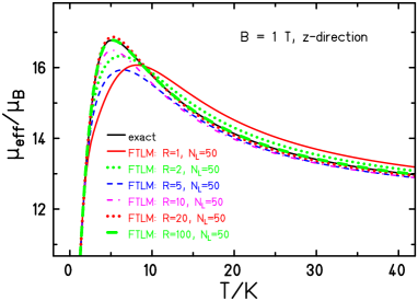
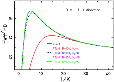
Figure 3: Effective magnetic moment of model system M1: The solid curves show the result of full matrix diagonalization, the broken curves show results of FTLM with reduced numbers of random vectors (top) and Lanczos steps (bottom).

In order to gain some insight into the influence of the two parameters $R$ and $N_{L}$ of the approximation, we performed simulations with a few different values. Figure 3 (top) shows how the approximation approaches the exact result as a function of $R$ for fixed $N_{L}=50$. One notices that even for a small number of random vectors low- and high-temperature part are already rather accurate, and that for an overall convergence $R\gtrsim 20$ (plus symmetry-related states) is already sufficient. The approximation for $R=100$ is indistinguishable from the exact result. The bottom part of Fig. 3 displays FTLM approximations for a few $N_{L}$ with fixed number of random vectors $R=100$. It is amazing how quickly the approximation approaches the exact result: for $N_{L}\gtrsim 15$ no deviation is visible any more.

Model system M2 is inspired by Mn${}_{6}^{\text{III}}$Cr${}^{\text{III}}$ molecules Hoeke et al. (2012b), where 6 spins $s=2$ are arranged in two equilateral triangles with fictitious nearest neighbor exchange interaction $J_{1}=\pm 0.314$ cm^-1 and a seventh central ion with $s=3/2$ connected with $J_{2}=-6.0$ cm^-1 to all other spins. The single-ion anisotropy tensors with $D_{i}=-5.0$ cm^-1, $E_{i}=0$ for the Mn spins are the same as in M1, compare Fig. 1; for chromium we choose $D_{7}=E_{7}=0$. The size of the Hilbert space is 62.500. The exact evaluation of a powder average with 25 orientations for just one field value needs about a week, thereby gobbling up 46 GB of RAM. The corresponding FTLM simulations need less than one hour on a simple notebook. Figure 4 displays again the effective magnetic moment along $z$-direction (top) and as a powder average (bottom). The solid curves show the result of full matrix diagonalization, the dashed ones the result of FTLM. Again, the accuracy is astonishing.

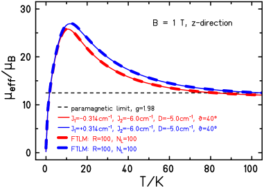
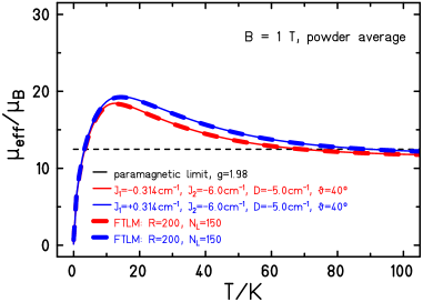
Figure 4: Effective magnetic moment of model system M2: moment along $z$-direction (top), powder averaged moment (bottom). The solid curves show the result of full matrix diagonalization, the dashed ones the result of FTLM.

This success is very encouraging for two reasons: With a numerically exact diagonalization it is virtually impossible to perform large parameter searches for molecules as big as M2, while using FTLM it becomes feasible. In addition, one can now numerically investigate much larger anisotropic spin systems both as function of temperature and field with high accuracy. This will be demonstrated in the following.

Several of the most interesting molecular magnets, i.e. magnetic molecules possessing a magnetic hysteresis, are of bigger size. The famous Mn₁₂-acetate molecules contain 12 manganese ions of two valencies (8 Mn³⁺ ions with $s=2$ and 4 Mn⁴⁺ ions with $s=3/2$) Lis (1980); Sessoli et al. (1993a, b); Thomas et al. (1996); Lionti et al. (1997); Thomas and Barbara (1998); Chiorescu et al. (2000). The resulting dimension of the Hilbert space assumes exactly 100,000,000. It was so far impossible to treat such a molecule on the basis of a full spin Hamiltonian including single-ion anisotropy. First attempts have been made using Lanczos procedures for low-lying states as well as high-temperature series expansions Regnault et al. (2002); Chaboussant et al. (2004). Other spin systems of similar size are the mixed valent Mn₁₂ ring of Christou Sessoli et al. (1993a) as well as the mono-valent Mn${}_{12}^{\text{III}}$ ring of Brechin Sanz et al. (2014).

Since it is our aim to demonstrate that the extension of FTLM towards anisotropic spin systems works we consider a fictitious Mn${}_{12}^{\text{III}}$ ring with uniaxial anisotropy. This has the advantage that at least for magnetic fields along the anisotropy axis we can compare FTLM codes employing $\!\hbox{}\mathop{\vphantom{S}\smash{S}}\limits_{\sim}\!{}^{z}$ symmetry with the new method. The Hamiltonian thus can be written as

$$\!\hbox{}\mathop{\vphantom{H}\smash{H}}\limits_{\sim}\hbox{}\! = -2\;J\;\sum_{i}\;\!\hbox{}\mathop{\vphantom{\vec{s}}\smash{\vec{s}}}\limits_{\sim}\!{}_{i}\cdot\!\hbox{}\mathop{\vphantom{\vec{s}}\smash{\vec{s}}}\limits_{\sim}\!{}_{i+1}+D\;\sum_{i}\;\left(\!\hbox{}\mathop{\vphantom{\vec{s}}\smash{\vec{s}}}\limits_{\sim}\!{}_{i}^{z}\right)^{2}$$

$$+g\,\mu_{B}\,\vec{B}\cdot\!\hbox{}\mathop{\vphantom{\vec{S}}\smash{\vec{S}}}\limits_{\sim}\hbox{}\!\ .$$

We investigated magnetic observables for several orientations of the external magnetic field for the following parameters of the spin system: $J=\pm 3.0$ cm^-1, $D=-1.8$ cm^-1, and $g=1.98$. The dimension of the Hilbert space is 244,140,625.

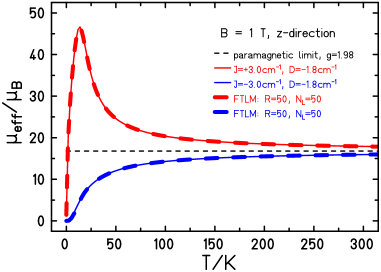
Figure 5: Effective magnetic moment of a fictitious Mn${}_{12}^{\text{III}}$: The solid curves are produced with a FTLM code employing spin rotational symmetry about the $z$-axis ($R=20,N_{L}=120$), whereas the broken curves are calculated with the method proposed in this article.

The case where the applied field points along the uniaxial anisotropies can be treated with a FTLM code where the Hilbert space is decomposed into subspaces ${\mathcal{H}}(M)$, compare Schnack and Wendland (2010); Schnack and Heesing (2013). The resulting effective magnetic moment is depicted by solid curves in Fig. 5. The effective moment for a ferromagnetic coupling shows the typical maximum, whereas for the antiferromagnetic case, the effective moment simply rises with increasing temperature. The dashed curves present the results of our proposed FTLM. The agreement is again very good.

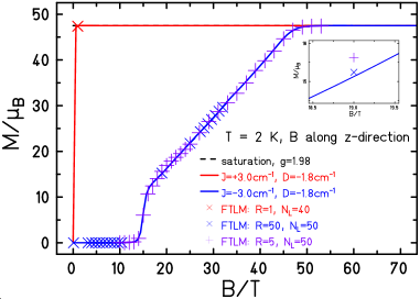
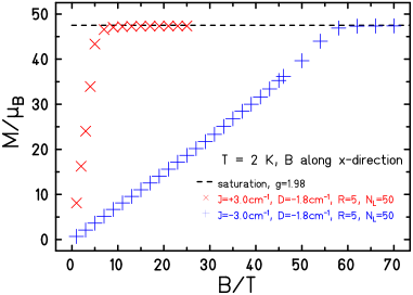
Figure 6: Magnetization of a fictitious Mn${}_{12}^{\text{III}}$: $B$ along $z$-direction (top), $B$ along $x$-direction (bottom). The solid curves are produced with a FTLM code employing spin rotational symmetry about the $z$-axis ($R=100,N_{L}=120$). The symbols depict the magnetization calculated with the method proposed in this article for various numbers of random vectors. The inset shows for a single data point with larger deviation how the numerical result improves when using 50 instead of 5 random vectors.

The magnetization is shown in Fig. 6 for $B$ pointing along $z$- and $x$-direction. In the ferromagnetic case the magnetization for a field along $z$-direction closely follows the Brillouin function of a total spin $S=24$, and thus immidiately jumps to saturation. In the antiferromagnetic case the staircase bahavior of a pure Heisenberg ring is smeared out due to anisotropy (and temperature). Both functions are rather well reproduced by the proposed FTLM. Nevertheless, now the evaluations need some time: a single data point with $R=5$ and $N_{L}=50$ needs about eight hours on 128 cores of our local SMP machine. Therefore, we evaluated only one data point for the ferromagnetic case, but several for the antiferromagnetic case, compare Fig. 6 (top). For the antiferromagnetic case we again investigated the influence of the number of random vectors $R$. We find that for $T=2$ K, which is of the order of the parameters of the Hamiltonian, five random vectors (and their symmetry related counterparts) are sufficient for most of the curve. Only around $B=20$ T, where we observe a small deviation, we find that an increased number of random vectors ($R=50$) is necessary to yield a good approximation, compare inset of Fig. 6 (top). As expected for a Monte-Carlo-type procedure the deviations are about $1/\sqrt{10}$ times smaller for 10 times more random vectors.

In the case where the external field is applied perpendicular to the easy axes, Fig. 6 (bottom), the magnetization rises more slowly both in the ferromagnetic as well as in the antiferromagnetic case. Observable such as this one cannot be evaluated with any other method (with the same accuracy).

V Summary and Outlook

After countless efforts to develop numerical strategies that rest on the symmetries of a quantum spin problem Delfs et al. (1993); Borras-Almenar et al. (1999); Waldmann (2000); Bostrem et al. (2006); Schnalle and Schnack (2009, 2010), nowadays approximate methods such as Quantum Monte Carlo Sandvik and Kurkijärvi (1991); Sandvik (1999); Engelhardt and Luban (2006), Density Matrix Renormalization Group Methods White (1993); Schollwöck (2005) and in particular Krylov space based methods such as FTLM produce approximate results of unprecedented accuracy. The latter is in particlar encouraging since Lanczos methods are very easy to program whereas irreducible representations of SU(2) combined with point groups have been mastered by only a rather small group of experts. In addition they don’t suffer from restrictions such as the negative sign problem that Quantum Monte Carlo faces for frustrated spin systems.

We thus hope that we could convince the reader that the Finite-Temperature Lanczos Method is capable of evaluating the thermal properties of large quantum spin systems even if they lack the $\!\hbox{}\mathop{\vphantom{S}\smash{S}}\limits_{\sim}\!{}^{z}$ symmetry.

References

- Gatteschi et al. (2006) D. Gatteschi, R. Sessoli, and J. Villain, Molecular Nanomagnets, Mesoscopic Physics and Nanotechnology (Oxford University Press, Oxford, 2006).
- Lis (1980) T. Lis, Acta Chrytallogr. B 36, 2042 (1980), URL http://dx.doi.org/10.1140/epjb/e2010-00028-3.
- Sessoli et al. (1993a) R. Sessoli, H. L. Tsai, A. R. Schake, S. Wang, J. B. Vincent, K. Folting, D. Gatteschi, G. Christou, and D. N. Hendrickson, J. Am. Chem. Soc. 115, 1804 (1993a), URL http://pubs.acs.org/doi/abs/10.1021/ja00058a027.
- Sessoli et al. (1993b) R. Sessoli, D. Gatteschi, A. Caneschi, and M. A. Novak, Nature 365, 141 (1993b), URL http://dx.doi.org/10.1038/365141a0.
- Thomas et al. (1996) L. Thomas, F. Lionti, R. Ballou, D. Gatteschi, R. Sessoli, and B. Barbara, Nature 383, 145 (1996), URL http://dx.doi.org/10.1038/383145a0.
- Gomes et al. (1998) A. Gomes, M. Novak, R. Sessoli, A. Caneschi, and D. Gatteschi, Phys. Rev. B 57, 5021 (1998), URL http://link.aps.org/doi/10.1103/PhysRevB.57.5021.
- Cornia et al. (2001) A. Cornia, M. Affronte, A. C. D. T. Gatteschi, A. G. M. Jansen, A. Caneschi, and R. Sessoli, J. Magn. Magn. Mater. 226, 2012 (2001), URL http://dx.doi.org/10.1016/S0304-8853(00)01093-3.
- Gatteschi and Sessoli (2003) D. Gatteschi and R. Sessoli, Angew. Chem., Int. Edit. 42, 268 (2003), URL http://dx.doi.org/10.1002/anie.200390099.
- Milios et al. (2007) C. J. Milios, A. Vinslava, W. Wernsdorfer, S. Moggach, S. Parsons, S. P. Perlepes, G. Christou, and E. K. Brechin, J. Am. Chem. Soc. 129, 2754 (2007), URL http://dx.doi.org/10.1021/ja068961m.
- Carretta et al. (2008) S. Carretta, T. Guidi, P. Santini, G. Amoretti, O. Pieper, B. Lake, J. van Slageren, F. E. Hallak, W. Wernsdorfer, H. Mutka, et al., Phys. Rev. Lett. 100, 157203 (2008), URL http://link.aps.org/abstract/PRL/v100/e157203.
- Glaser et al. (2009) T. Glaser, M. Heidemeier, E. Krickemeyer, H. Bögge, A. Stammler, R. Fröhlich, E. Bill, and J. Schnack, Inorg. Chem. 48, 607 (2009), URL http://pubs.acs.org/doi/abs/10.1021/ic8016529.
- Glaser (2011) T. Glaser, Chem. Commun. 47, 116 (2011), URL http://dx.doi.org/10.1039/C0CC02259D.
- Hoeke et al. (2012a) V. Hoeke, M. Heidemeier, E. Krickemeyer, A. Stammler, H. Bögge, J. Schnack, and T. Glaser, Dalton Trans. 41, 12942 (2012a), URL http://dx.doi.org/10.1039/C2DT31590D.
- Hoeke et al. (2012b) V. Hoeke, M. Heidemeier, E. Krickemeyer, A. Stammler, H. Bögge, J. Schnack, A. Postnikov, and T. Glaser, Inorg. Chem. 51, 10929 (2012b), URL http://pubs.acs.org/doi/abs/10.1021/ic301406j.
- Hoeke et al. (2013) V. Hoeke, E. Krickemeyer, M. Heidemeier, H. Theil, A. Stammler, H. Bögge, T. Weyhermüller, J. Schnack, and T. Glaser, Eur. J. of Inorg. Chem. 2013, 4398 (2013), URL http://dx.doi.org/10.1002/ejic.201300400.
- Hoeke et al. (2014) V. Hoeke, A. Stammler, H. Bögge, J. Schnack, and T. Glaser, Inorg. Chem. 53, 257 (2014), URL http://pubs.acs.org/doi/abs/10.1021/ic4022068.
- Jaklic and Prelovsek (1994) J. Jaklic and P. Prelovsek, Phys. Rev. B 49, 5065 (1994), URL http://dx.doi.org/10.1103/PhysRevB.49.5065.
- Jaklic and Prelovsek (2000) J. Jaklic and P. Prelovsek, Adv. Phys. 49, 1 (2000), URL http://dx.doi.org/10.1080/000187300243381.
- Manthe and Huarte-Larranaga (2001) U. Manthe and F. Huarte-Larranaga, Chem. Phys. Lett. 349, 321 (2001), URL http://www.sciencedirect.com/science/article/pii/S00092614010%12076.
- Long et al. (2003) M. W. Long, P. Prelovšek, S. El Shawish, J. Karadamoglou, and X. Zotos, Phys. Rev. B 68, 235106 (2003), URL http://link.aps.org/doi/10.1103/PhysRevB.68.235106.
- Aichhorn et al. (2003) M. Aichhorn, M. Daghofer, H. G. Evertz, and W. von der Linden, Phys. Rev. B 67, 161103 (2003), URL http://dx.doi.org/10.1103/PhysRevB.67.161103.
- Shannon et al. (2004) N. Shannon, B. Schmidt, K. Penc, and P. Thalmeier, Eur. Phys. J. B 38, 599 (2004), URL http://dx.doi.org/10.1140/epjb/e2004-00156-3.
- Zerec et al. (2006) I. Zerec, B. Schmidt, and P. Thalmeier, Phys. Rev. B 73, 245108 (2006), URL http://link.aps.org/abstract/PRB/v73/e245108.
- Schmidt et al. (2007) B. Schmidt, P. Thalmeier, and N. Shannon, Phys. Rev. B 76, 125113 (2007), URL http://dx.doi.org/10.1103/PhysRevB.76.125113.
- Siahatgar et al. (2012) M. Siahatgar, B. Schmidt, G. Zwicknagl, and P. Thalmeier, New J. Phys. 14, 103005 (2012), URL http://dx.doi.org/10.1088/1367-2630/14/10/103005.
- Jaklič and Prelovšek (1994) J. Jaklič and P. Prelovšek, Phys. Rev. B 50, 7129 (1994), URL http://link.aps.org/doi/10.1103/PhysRevB.50.7129.
- Schnack and Wendland (2010) J. Schnack and O. Wendland, Eur. Phys. J. B 78, 535 (2010), URL http://dx.doi.org/10.1007/BF01609348.
- Schnack and Heesing (2013) J. Schnack and C. Heesing, Eur. Phys. J. B 86, 46 (2013), URL http://dx.doi.org/10.1140/epjb/e2012-30546-7.
- Zheng et al. (2013) Y. Zheng, Q.-C. Zhang, L.-S. Long, R.-B. Huang, A. Müller, J. Schnack, L.-S. Zheng, and Z. Zheng, Chem. Commun. 49, 36 (2013), URL http://dx.doi.org/10.1039/C2CC36530H.
- Lanczos (1950) C. Lanczos, J. Res. Nat. Bur. Stand. 45, 255 (1950), URL http://dx.doi.org/10.6028/jres.045.026.
- Regnault et al. (2002) N. Regnault, T. Jolicœur, R. Sessoli, D. Gatteschi, and M. Verdaguer, Phys. Rev. B 66, 054409 (2002), URL http://link.aps.org/doi/10.1103/PhysRevB.66.054409.
- Chaboussant et al. (2004) G. Chaboussant, A. Sieber, S. Ochsenbein, H.-U. Güdel, M. Murrie, A. Honecker, N. Fukushima, and B. Normand, Phys. Rev. B 70, 104422 (2004), URL http://link.aps.org/doi/10.1103/PhysRevB.70.104422.
- Schnack et al. (2008) J. Schnack, P. Hage, and H.-J. Schmidt, J. Comput. Phys. 227, 4512 (2008), URL http://dx.doi.org/10.1016/j.jcp.2008.01.027.
- Schmidt et al. (2001) H.-J. Schmidt, J. Schnack, and M. Luban, Phys. Rev. B 64, 224415 (2001), URL http://dx.doi.org/10.1103/PhysRevB.64.224415.
- Thuesen et al. (2010) C. A. Thuesen, H. Weihe, J. Bendix, S. Piligkos, and O. Monsted, Dalton Trans. 39, 4882 (2010), URL http://dx.doi.org/10.1039/B925254A.
- Schmidt et al. (2011) H.-J. Schmidt, A. Lohmann, and J. Richter, Phys. Rev. B 84, 104443 (2011), URL http://link.aps.org/doi/10.1103/PhysRevB.84.104443.
- Lohmann et al. (2014) A. Lohmann, H.-J. Schmidt, and J. Richter, Phys. Rev. B 89, 014415 (2014), URL http://link.aps.org/doi/10.1103/PhysRevB.89.014415.
- Glaser et al. (2010) T. Glaser, M. Heidemeier, H. Theil, A. Stammler, H. Bögge, and J. Schnack, Dalton Trans. 39, 192 (2010), URL http://dx.doi.org/10.1039/b912593k.
- Lebedev and Laikov (1999) V. I. Lebedev and D. N. Laikov, Dokl. Akad. Nauk 366, 741 (1999).
- Lionti et al. (1997) F. Lionti, L. Thomas, R. Ballou, B. Barbara, A. Sulpice, R. Sessoli, and D. Gatteschi, J. Appl. Phys. 81, 4608 (1997), URL http://dx.doi.org/10.1063/1.365177.
- Thomas and Barbara (1998) L. Thomas and B. Barbara, J. Low Temp. Phys. 113, 1055 (1998), URL http://dx.doi.org/10.1023/A:1022516703754.
- Chiorescu et al. (2000) I. Chiorescu, R. Giraud, A. G. M. Jansen, A. Caneschi, and B. Barbara, Phys. Rev. Lett. 85, 4807 (2000), URL http://link.aps.org/doi/10.1103/PhysRevLett.85.4807.
- Sanz et al. (2014) S. Sanz, J. M. Frost, T. Rajeshkumar, S. J. Dalgarno, G. Rajaraman, W. Wernsdorfer, J. Schnack, P. J. Lusby, and E. K. Brechin, Chem. Eur. J. 20, 3010 (2014), URL http://dx.doi.org/10.1002/chem.201304740.
- Delfs et al. (1993) C. Delfs, D. Gatteschi, L. Pardi, R. Sessoli, K. Wieghardt, and D. Hanke, Inorg. Chem. 32, 3099 (1993), URL http://pubs.acs.org/doi/abs/10.1021/ic00066a022.
- Borras-Almenar et al. (1999) J. J. Borras-Almenar, J. M. Clemente-Juan, E. Coronado, and B. S. Tsukerblat, Inorg. Chem. 38, 6081 (1999), URL http://dx.doi.org/10.1021/ic990915i.
- Waldmann (2000) O. Waldmann, Phys. Rev. B 61, 6138 (2000), URL http://link.aps.org/doi/10.1103/PhysRevB.61.6138.
- Bostrem et al. (2006) I. G. Bostrem, A. S. Ovchinnikov, and V. E. Sinitsyn, Theor. Math. Phys. 149, 1527 (2006).
- Schnalle and Schnack (2009) R. Schnalle and J. Schnack, Phys. Rev. B 79, 104419 (2009), URL http://link.aps.org/abstract/PRB/v79/e104419.
- Schnalle and Schnack (2010) R. Schnalle and J. Schnack, Int. Rev. Phys. Chem. 29, 403 (2010), URL http://dx.doi.org/10.1080/0144235X.2010.485755.
- Sandvik and Kurkijärvi (1991) A. W. Sandvik and J. Kurkijärvi, Phys. Rev. B 43, 5950 (1991), URL http://link.aps.org/doi/10.1103/PhysRevB.43.5950.
- Sandvik (1999) A. W. Sandvik, 59, R14157 (1999), URL http://link.aps.org/doi/10.1103/PhysRevB.59.R14157.
- Engelhardt and Luban (2006) L. Engelhardt and M. Luban, Phys. Rev. B 73, 054430 (2006), URL http://link.aps.org/doi/10.1103/PhysRevB.73.054430.
- White (1993) S. R. White, Phys. Rev. B 48, 10345 (1993), URL http://link.aps.org/doi/10.1103/PhysRevB.48.10345.
- Schollwöck (2005) U. Schollwöck, Rev. Mod. Phys. 77, 259 (2005), URL http://link.aps.org/doi/10.1103/RevModPhys.77.259.