Characterizing the Topography of Multi-dimensional Energy Landscapes

Abstract

A basic issue in optimization, inverse theory, neural networks, computational chemistry and many other problems is the geometrical characterization of high dimensional functions. In inverse calculations one aims to characterize the set of models that fit the data (among other constraints). If the data misfit function is unimodal then one can find its peak by local optimization methods and characterize its width (related to the range of data-fitting models) by estimating derivatives at this peak. On the other hand, if there are local extrema, then a number of interesting and difficult problems arise. Are the local extrema important compared to the global or can they be eliminated (e.g., by smoothing) without significant loss of information? Is there a sufficiently small number of local extrema that they can be enumerated via local optimization? What are the basins of attraction of these local extrama? Can two extrema be joined by a path that never goes uphill? Can the whole problem be reduced to one of enumerating the local extrema and their basins of attraction? For locally ill-conditioned functions, premature convergence of local optimization can be confused with the presense of local extrema. Addressing any of these issues requires topographic information about the functions under study. But in many applications these functions may have hundreds or thousands of variables and can only be evaluated pointwise (by some numerical method for instance). In this paper we describe systematic (but generic) methods of analysing the topography of high dimensional functions using local optimization methods applied to randomly chosen starting models. We provide a number of quantitative measures of function topography that have proven to be useful in practical problems along with error estimates.

I What Makes an Optimization Problem Hard?

We consider the problem of optimizing a function $F$ (the objective or cost function) mapping ${\cal M}\subset{\bf R}^{N}$ into ${\cal Y}\subset{\bf R}$. We refer to ${\cal M}$ as the model space, and each point in the model space, ${\bf m}$, is a model. Depending on the application, the goal may be to find the global extremum of $F$, a single local extremum, or a collection of local extrema. In this paper we will assume that optimization refers to minimization, whether local or global.

There is no generally agreed upon characterization of what makes an optimization problem hard. Hardness has to do partly with our goals — do we need a global extremum or will a good local extremum do; partly with the structure of the function — does it have lots of local extrema, how broad are the basins associated with these extrema; and partly with the dimensionality of the problem — exhaustive search will be infeasible except for low-dimensional problems.

In many applications, however, the function $F$ cannot be expressed in closed form in terms of elementary functions, but can only be evaluated point-wise by computer programs. Such problems arise in many fields. Some of the most widely studied include the spin-glass problem, the traveling-salesman problem (TSP), and the residual statics problem of exploration seismology.

I.1 Global Search Strategies

If the structure of function $F$ is unknown, optimization is fundamentally a matter of search in the model space. In order to be able to treat such a broad variety of situations, we begin with an abstract statement of a search algorithm. Here, we use the notation ${\bf{\vec{m}}}^{t}$ to represent a population of candidate models at the time step $t$.

Algorithm 1

General Search (GS) ${\bf{\vec{m}}}={\mathit{G}S}(F,P,{\bf T},S)$
Let $F:{\cal M}\subset{\bf R}^{N}\rightarrow{\cal Y}\subset{\bf R}$, $P\equiv{\bf{\vec{m}}}^{0}=\{{\bf m}^{0}_{k}\}_{k=1,\cdots,K}$ be an initial population of models, where ${\bf m}^{0}_{k}\in{\cal M}$ and $K\geq 1$, ${\bf T}$ a transition operator, and $S$ a stopping criterion.

1. Iteratively apply the transition operator to generate a new population of models at each iteration, so that ${\bf{\vec{m}}}^{t}={\bf T}\,{\bf{\vec{m}}}^{t-1};$

2. Repeat (1) until $S$ is satisfied. The final set of models ${\bf{\vec{m}}}$ are the output of the search.

Any searching process can be considered as an evolution of a population of models (possibly a single model) in the $N$-dimensional model space. The transition operator ${\bf T}$ is the rule that determines to which models the population evolves from the previous population. Here, we assume that the transition operator ${\bf T}$ is independent of the time step $t$, which is the case in most algorithms. Different optimization algorithms differ by the strategies in choosing the initial population $P$ and the rules of transition from one population of models to another, ${\bf T}$.

Among the searching methods defined via Algorithm 1, there are two extreme strategies, hill-climbing (HC) and uniform Monte Carlo (UMC). HC search is a local descent search applied to a single model (population size $K=1$). An initial model $P={\bf m}^{0}$ is selected (possibly at random) and the transition operators ${\bf T}={\bf T}_{local}$ are deterministic operators, such as conjugate gradient, quasi-Newton, or downhill simplex, which follow a path downhill as far as possible. For objective functions containing more than one local extremum (multi-modal), the result of HC strongly depends on the choice of the initial model ${\bf m}^{0}$. UMC, on the other hand, selects points with uniform probability in the model space. The transition operation ${\bf T}$ is simply the selection of new points at random and therefore makes no use of information from previous generations. Thus, if there are $N$ parameters and each of them can take $m$ possible values, the probability of finding a particular model is proportional to $m^{-N}$ for each function evaluation using UMC.

Search strategies have been developed that yield a compromise between these two extremes; almost all of these incorporates stochastic elements, especially in the construction of transition operators. It is important for the success of global searches that the transition operators make the best use of information provided by the current samples while avoiding being trapped in local extrema. Among all these strategies, the most widely used are Simulated Annealing (SA) kirkpatrick , Genetic Algorithms (GA) holland and random hill-climbing (RHC), to be defined shortly.

SA and GA searching strategies use stochastic transition operators ${\bf T}$ that are biased towards good samples from the previous generations. Many variations of SA and GA can be found in the literature aarts:book ; vanlaarhoven ; goldberg:book . Although the asymptotic convergence results are known for both SA hajek and GA davis_principe these results are hardly useful in practice.

RHC searches, on the other hand, apply deterministic transition operations ${\bf T}$ to a randomly chosen population $P$. Hence RHC explores locally in multiple areas of objective functions, and the resulting samples are a set of local/global extrema. This search algorithm can be described as

Algorithm 2

Random Hill Climbing ${\bf{\vec{m}}}={\mathit{R}HC}(F,K,\epsilon,cmax)$
Let the randomly chosen initial population size be $K$. Let the stopping criterion $S$ be that either gradients of all samples are reduced to the tolerance $\epsilon$ or the number of iterations reaches a maximum $cmax$. Let ${\bf T}_{local}$ be a local descent search operator.

1. Choose initial models $P=\{{\bf m}^{0}_{k}\}_{k=1,\cdots,K}\in{\cal M}$ uniformly at random, where $K\gg 1$;

2. Apply Algorithm 1, ${\bf{\vec{m}}}={\mathit{G}S}(F,P,{\bf T}_{local},S)$.

The final population contains $n$ distinct models, ${\bf{\vec{m}}}=\{{\bf m}_{k}\}_{k=1,\cdots,n}$.

By uniformly random we mean that each components of the initial models are chosen randomly with uniformly probability between the maximum and minimum possible values. In this paper, all RHC numerical results use non-linear Conjugate Gradient as transition operators coool .

I.2 Landscape of Objective Functions

Chavent curvature2 developed sufficient conditions for an objective function to be locally convex. These conditions are based on the distance $\times$ curvature induced by the objective function on trajectories. In principle, this local convexity criterion could be generalized to global samples of an objective function, to provide a global measure of complexity.

On the other hand, imagine the surface of an objective function being a high-dimensional landscape with hills and basins of different depths and widths scattered on the surface. Performance of searching algorithms depends to a large extent on topographical features on this landscape.

For SA and GAs, this situation is summarized heuristically by Kaufmann kaufmann2 :

“Annealing works well only in landscapes in which deep energy wells also drain wide basins. It does not work well on either a random landscape or a “golf course” potential, which is flat everywhere except for a unique “hole”. In the latter case, the landscape offers no clue to guide search.

Recombination (in GAs) is useless on uncorrelated landscapes but useful under two conditions (1) when the high peaks are near one another and hence carry mutual information about their joint locations in genotype space and (2) when parts of the evolving system are quasi-independent of one another and hence can be interchanged with modest chances that the recombined system had the advantage of both parents.”

In addition, since RHC uses local-descent transition operators, its performance will also be strongly influenced by topography.

It has been proposed that functions can be characterized by their spatial correlation properties weinberger ; stadler2 . Several typical combinatorial optimization problems have been investigated by studying the correlation in landscapes: the TSP stadler4 , graph-bipartitioning problem stadler1 , and the $NK$ model problems, a spin-glass like problem in biology kaufmannweinberger . Using correlation features of the objective function’s landscape as a criterion, these authors study the effectiveness of particular global algorithms for certain types of landscapes.

In addition, analyzing the topography of high-dimensional energy functions is important in physics and chemistry. Berry and Breitengraser-Kunz prl_topo studied topography and dynamics of multidimensional inter-atomic potential surfaces by analyzing a population of local minima, each of which has two saddle points connected to it. By connecting these samples in a certain order, the high-dimensional function surface is represented by a series of one-dimensional lines. By looking at these one-dimensional plots, the topography information is represented by the width and depth of the primary, secondary or tertiary basins of attractions prl_topo .

The structure of high-dimensional Hamiltonians has also been studied by means of entropy prl_entropy . For an $N$-dimensional Hamiltonian, a collection of local extrema are first found by some means. Contributions of these local-minima are represented by a probability distribution $\{p_{i}\}_{i=1,\cdots,n}$ where

$$p_{i}\propto\Delta^{(i)}(N)=\prod_{k=1}^{N}\delta^{i}_{k}.$$ (1)

Here, $\delta^{i}_{k}$ is the estimated width of the $i$th basin of attraction along the $k$th coordinate. The $N$-dimensional surface is then characterized by the following entropy,

$$S(N)=-\sum_{i}p_{i}\ln p_{i}=\left\langle\ln\left(\frac{1}{\Delta(N)}\right)\right\rangle.$$ (2)

In this paper, we use a similar measure. However, we estimate $p_{i}$ by random hill-climbing rather than equation 1. Further, we base our measure not on $p_{i}$ itself, but rather on a related probability that takes into account of the values of the local minima. We also perform a confidence interval analysis. Finally, as a concrete application, we show that this measure can be used to compute the optimal simplification of a multi-resolution analysis (MRA) of highly non-convex seismic optimization problem.

II Measures of Topography

II.1 Definitions

The surface topography of functions is largely associated with the number of local minima, widths of the basin of attractions associated with these minima, and relative depths of these basins. The basin of attraction associated with the $i$th local minimum may be loosely defined as the maximum volume $A_{i}$ in the $N$-dimensional model space within which all models can converge to the $i$th local minima after infinite number of iterations by a local descent search algorithm. Suppose the volume of the entire model space is represented as $M$, then the ratio $p_{i}=\frac{A_{i}}{M}$ is the probability of converging to the $i$th local minimum for a uniformly random model. The following definition serves to introduce three quantitative measures of topography: a probability associated with the relative volumes of the basins of attraction ($p$), a version of $p$ scaled by the estimated depths of the basins of attractions ($q$) and the entropy of $q$.

Definition 1

Entropy-Based Topography
Let $F:{\cal M}\subset{\bf R}^{N}\rightarrow{\cal Y}\subset{\bf R}$ be bounded and have $n$ isolated local minima, where $n$ is finite. Let $\{{\bf m}_{i}\}_{i=1,\cdots,n}$ be these distinct local minima, and $\{y_{i}=F({\bf m}_{i})\}_{i=1,\cdots,n}$ be their corresponding function values. Let $p_{i}$ be the probability that a model chosen with uniform probability in ${\cal M}$ will converge to the $i$th local minimum under the action of an exact local optimization algorithm.

Define $\{q_{i}\}_{i=1,\dots,n}$ to be a probability distribution where

$$q_{i}\propto\begin{cases}p_{i},&\hbox{if}\;\sigma=0;\cr p_{i}\,e^{-\frac{|y_{i}-y_{m}|}{\sigma}},&\hbox{otherwise},\cr\end{cases}$$ (3)

where $i\in[1,n]$, $y_{m}$ is the value at the global minimum, $\sigma=\frac{1}{n}\sum_{j=1}^{n}|y_{j}-y_{m}|$, and $\sum_{i=1}^{n}q_{i}=1$. The entropy is defined to be,

$$C_{e} = -\sum_{i=1}^{n}q_{i}\ln(q_{i})$$ (4)

$$= \left\langle\ln\left(\frac{1}{q_{i}}\right)\right\rangle,$$

where the angle brackets denote the expected value with respect to the probability distribution $\{q_{i}\}_{i=1,\dots,n}$.

For the entropy in Definition 1, it is always the case that $C_{e}\geq 0$. If the function is unimodal (only one extremum), then $C_{e}=0$. On the other hand, if the function has $n$ isolated and equally valued local extrema, then $C_{e}$ is $\ln n$. Therefore, the entropy increases with the number of local extrema $n$.

As a simple example, Figure 1 shows two one-dimensional functions with the same number of local minima and widths of basins of attractions ($A_{i}\propto p_{i}$). However, the difficulty of minimizing these functions is different: the left function has identical basins of attractions, while the one on the right has a dominant global minimum at $x=0$ and decreasingly important local minima away from the center. The entropy of Definition 1 gives a higher $C_{e}$ value to that of the function on the left ($C_{e}=2.2$) than that on the right ($C_{e}=1.5$).

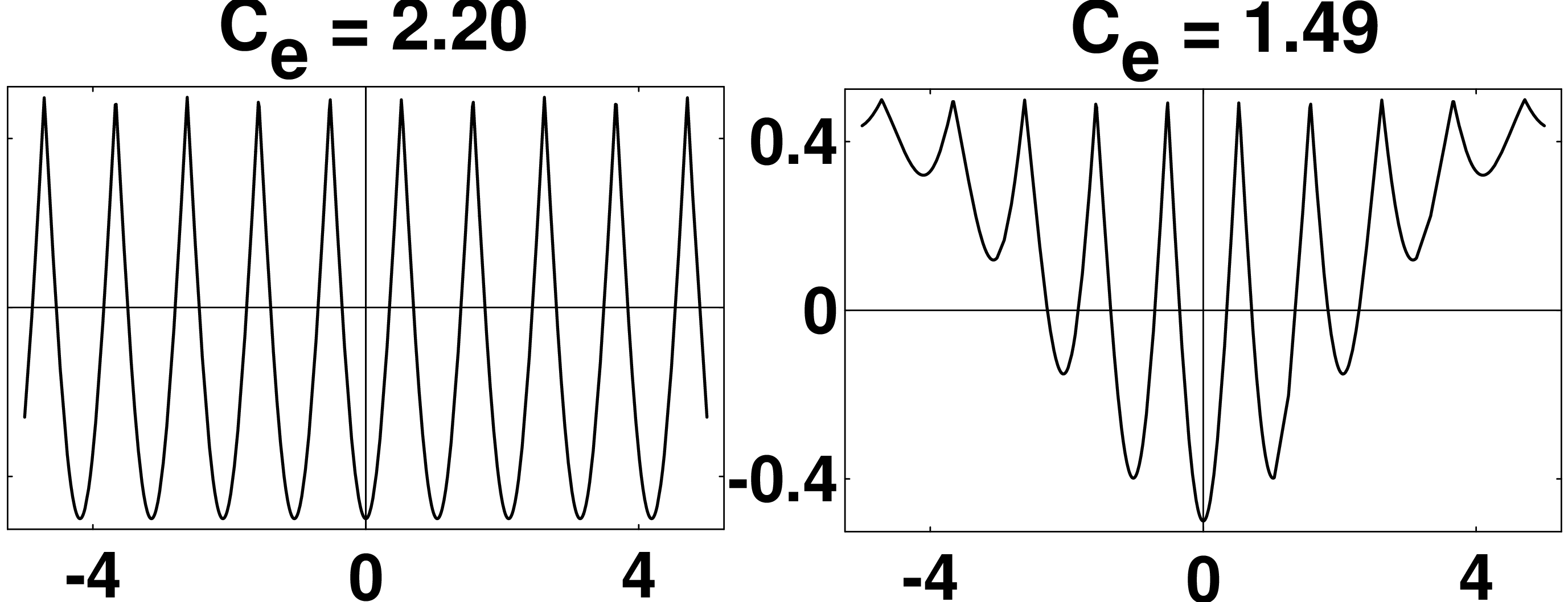
Figure 1: Two one-dimensional functions with the same number and widths of basins of attractions. The function on the left have entropy $C_{e}=2.2$, while the function on the right has $C_{e}=1.5$.

Since the functions we are interested in can usually be evaluated only point-wise, the number of local minima $n$ and $\{p_{i}\}_{i=1.\dots,n}$ are not known. Some degree of global sampling is essential in order to achieve the characterization we seek. As shown in Algorithm 2, RHC explores various regions of the model space and takes initial samples down-hill to the bottom of the basins on the surface of functions. Therefore, a statistical analysis of results of systematic RHC searches can be used to estimate the topographic quantities.

Suppose the local-descent search is ideal, i.e. all initial models converge to exact local minima, the number of models converging to each local minima from $K$ randomly chosen initial models has a multinomial probability distribution. If the initial models are randomly chosen under a uniform probability distribution, the probability of converging to the $i$th local minimum is proportional to the width of the $i$th basin of attraction, $p_{i}$. Let $K_{1},\dots,K_{n}$ be the random variables representing the frequency of models converging to each of the local minima. For the population of $K$, the joint probability density of these random variables is

$$f(k_{1},\dots,k_{n})=\frac{K!}{k_{1}!,\dots,k_{n}!}\;p_{1}^{k_{1}}\dots p_{n}^{k_{n}},$$ (5)

where $\sum_{i=1}^{n}k_{i}=K$. For each $i\in[1,n]$, the mean value of the random variable $k_{i}$ is $E[k_{i}]=K\,p_{i}$. Therefore, the convergence frequency of a RHC of large population can be used to estimate the number of local minima as well as the widths of basin of attractions. Hence, the estimation of the entropy measure in Definition 1 can be defined as follows.

Definition 2

Entropy-Based Estimates
Let $F:{\cal M}\subset{\bf R}^{N}\rightarrow{\cal Y}\subset{\bf R}$ be bounded and have finite number of isolated local minima. Let $\{{\bf m}_{i}\}_{i=1,\cdots,\hat{n}}={\bf RHC}(F,K,\epsilon,cmax)$ be the distinct converged models of RHC searches. Let $\{k_{i}\}_{i=1,\cdots,\hat{n}}$ be the frequency distribution of the final population, and $\{y_{i}=F({\bf m}_{i})\}_{i=1,\cdots,\hat{n}}$ be their corresponding function values.

Define the estimated entropy ${\hat{C}}_{e}$ as

$${\hat{C}}_{e} = -\sum_{i=1}^{\hat{n}}{\hat{q}}_{i}\ln({\hat{q}}_{i})$$ (6)

$$= \left\langle\ln\left(\frac{1}{{\hat{q}}_{i}}\right)\right\rangle,$$

where ${\hat{q}}_{i}$ is normalized to a probability distribution $\sum_{i=1}^{\hat{n}}{\hat{q}}_{i}=1,$ and ${\hat{q}}_{i}\propto x_{i}\,v_{i},$ in which

$$x_{i} \equiv \frac{k_{i}}{K},$$ (7)

and

$$v_{i}\equiv\begin{cases}1,&\hbox{if}\;\sigma=0;\cr\exp(-\frac{|y_{i}-y_{m}|}{\sigma}),&\hbox{otherwise},\cr\end{cases}$$ (8)

where $y_{m}=\min{\{y_{i}\}}$ and $\sigma=\frac{1}{{\hat{n}}}\sum_{j=1}^{\hat{n}}|y_{j}-y_{m}|$.

Definition 2 is a statistical estimation of the entropy in Definition 1. The exact entropy $C_{e}$ characterizes topographical features of objective function, and hence independent of numerical computation and any searching technique. The estimation ${\hat{C}}_{e}$, however, would be influenced by numerical issues. If, for examples, the curvature of the function is nearly zero, which is equivalent to an ill-conditioned Hessian matrix, gradient-based local descent searches may not converge to the exact local minima. The estimated value of ${\hat{C}}_{e}$ in such a situation may be higher than the true complexity $C_{e}$. In practice, however, it is often difficult to distinguish the results of such ill-conditioning from those of multi-modality. Therefore, taking such numerical issues into account can represent an important aspect in the difficulty of optimization.

II.2 Numerical Examples

In this section, we use the entropy ${\hat{C}}_{e}$ to study two commonly used test functions in optimization, the Rosenbrock and Griewank functions.

II.2.1 $N$-dimensional Rosenbrock function

An $N$-dimensional Rosenbrock function can be written as

$$R({\bf x})=\sum_{i=1}^{N-1}\left[100(x_{i}-x_{i-1}^{2})^{2}+(1-x_{i-1})^{2}\right],$$ (9)

where ${\bf x}=(x_{0},\;\dots,\;x_{N})$. Although unimodal, the long and narrow basin is a challenge for searching algorithms. Figure 2 shows the function surface and its contour when $N=2$. When $N\geq 2$, the function is still unimodal, but it is not easy to see how the increase of dimensionality alters the difficulty of optimization.

One way of studying the spatial curvature of functions is by looking at the ratio of largest and smallest eigenvalues (condition number) of the Hessian at a point. The Hessian for equation (9) is a tri-diagonal matrix,

$$\left(\begin{array}[]{ccccc}a_{0}&c_{0}&0&\cdots&0\\ b_{1}&a_{1}&c_{1}&0&\cdots\\ 0&b_{2}&a_{2}&c_{2}&0\\ \vdots&\vdots&\vdots&\vdots&\vdots\\ 0&0&\cdots&b_{N-1}&a_{N-1}\end{array}\right)$$ (15)

where

$$a_{i} = \begin{cases}2+1200\,x_{0}^{2}-400\,x_{1},&\hbox{if}\;i=0;\cr 202+1200x_{i-1}^{2}-400x_{i},&\hbox{if}$0 < i < N-1$;\cr 200,&\hbox{if}i=N-1,\cr\end{cases}$$

$$b_{i} = -400\,x_{i-1},\;\;\;\;0<i\leq N-1,$$

$$c_{i} = -400\,x_{i+1},\;\;\;\;0\leq i<N-1.$$

At the global minimum $(1,\,1,\,\cdots,\,1)$, the tri-diagonal matrix equation (15) becomes Toeplitz except for $a_{0}$ and $a_{N-1}$. The condition number of the Hessian at the global minimum reaches an asymptote with increasing dimension, as shown in Figure 3. Figure 4 shows ${\hat{C}}_{e}$ as a function of the number of dimensions; it shows the same asymptotic trend as does the condition number. Thus the increasing complexity for low dimensions is the result of increasing ill-conditioning of the Hessian and has nothing to do with local minima.

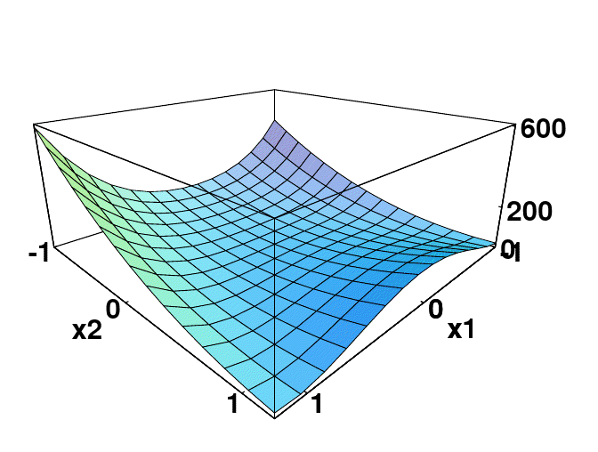
Figure 2: Two-dimensional Rosenbrock function. The figure on the left is a 3-D plot of the function surface, while the one on the right shows the contour plot of the same function.

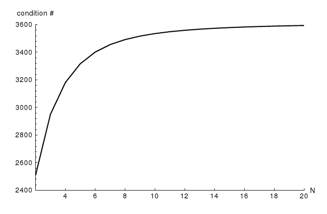
Figure 3: Condition number of the Hessian matrix for the N-dimensional Rosenbrock function at the global minimum.

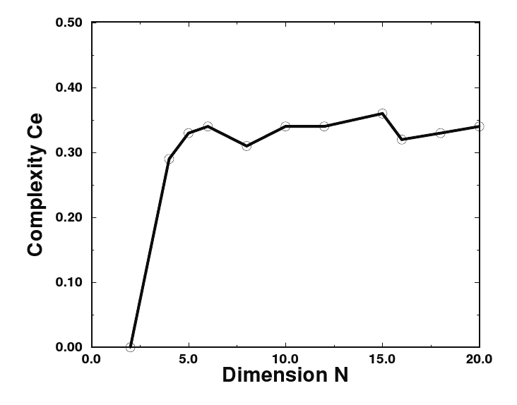
Figure 4: ${\hat{C}}_{e}$ for N-dimensional Rosenbrock functions as a function of $N$.

II.2.2 High-dimensional Griewank functions

The Griewank function is also used to test optimization algorithms whitley_testfcn2 ; torn-zilinska :

$$g({\bf x})=1+\sum_{i=1}^{N}\frac{x_{i}^{2}}{4000}-\prod_{i=1}^{N}\cos\left(\frac{x_{i}}{\sqrt{i}}\right)$$ (16)

The cosine term makes equation (16) multi-modal. Figure 5 shows a one-dimensional slice of the Griewank function along the diagonal of the hypercube for dimensions $1,3,5,9$. Whitley et al. whitley_testfcn2 observed such slices and concluded that “as the dimensionality increases the local optima induced by the cosine decrease in number and complexity”.

However, such pictures can be misleading since they tell us only about low-dimensional projections of the function. Figure 6 shows slices of the same functions when all but one variables are fixed to be $0$. The increasing dimensionality does not change the oscillation around the global minimum at the origin. Therefore, studying the overall performance of high dimensional functions could be tricky. We compute ${\hat{C}}_{e}$ for the Griewank function with a population $500$ and $1000$ models in the hyper-cube of $-10\leq x_{i}\leq 10,\;\;\;i=0,\cdots,N-1$. Figure 7 shows the resulting ${\hat{C}}_{e}$ for dimensions up to $50$ for initial populations of both $500$ and $1000$. Both curves in Figure 7 give us consistent results that the complexity of Griewank function in this range increases till dimension around $9$, then decreases when number of dimension continuous to increase. This result can be verified by the analysis of Griewank function. Therefore, using the entropy we can understand more comprehensively the dimensional-dependence of complexity of certain functions than by simply looking at hyper-planes.

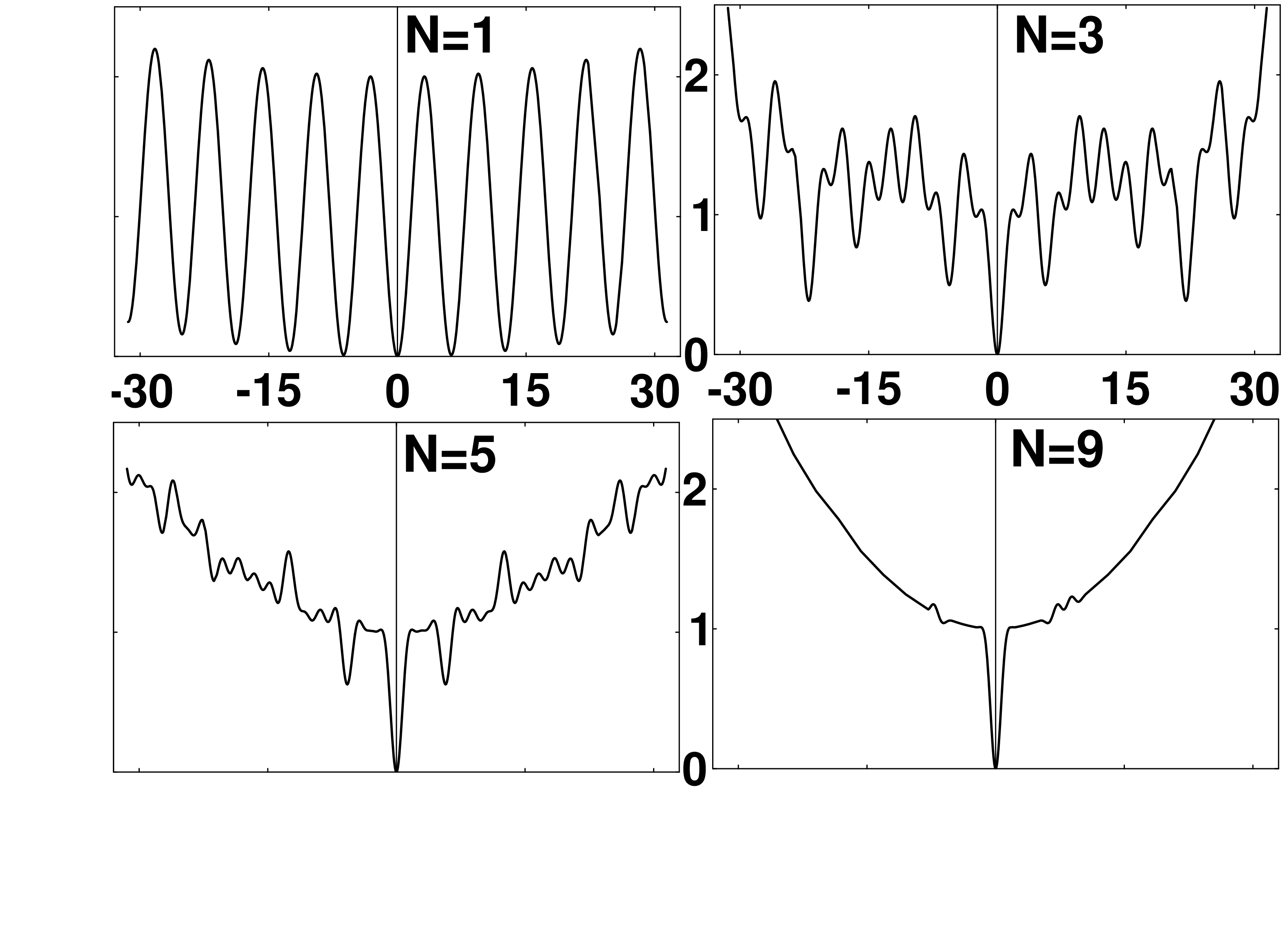
Figure 5: Diagonal slices of $N$-dimensional Griewank functions.

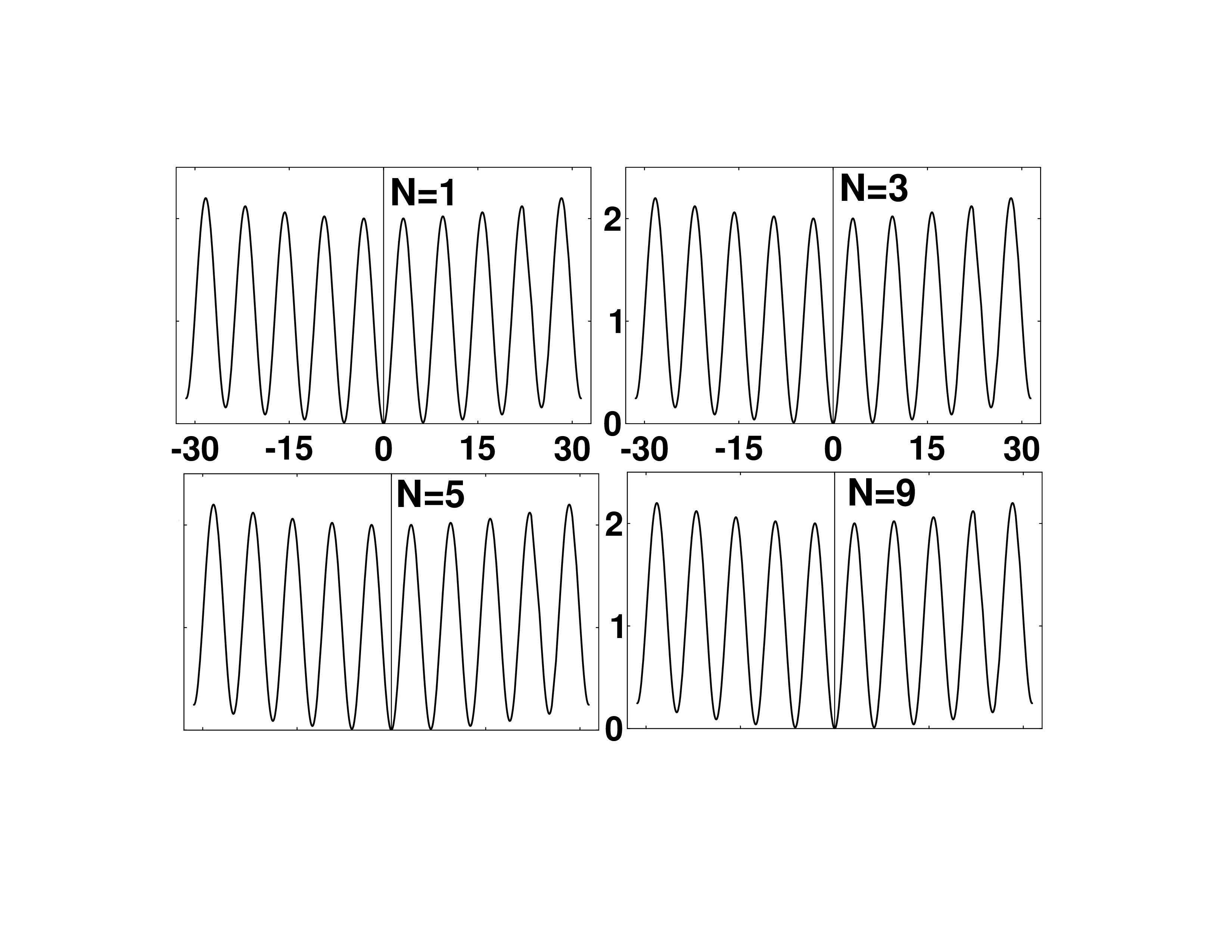
Figure 6: Slices of $N$-dimensional Griewank functions. All variables but one are fixed at $0$.

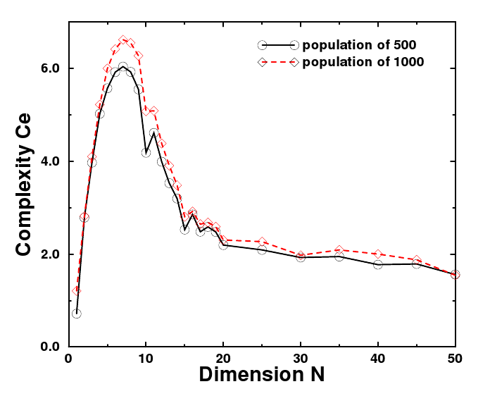
Figure 7: $\hat{C_{e}}$ as a function of dimension $N$ for the Griewank function with populations of $500$ and $1000$.

III Confidence Intervals Analysis

Next we derive confidence intervals on the entropy in Definition 2. The following analysis is based on the assumption of ideal RHC, which is a special case of Algorithm 2 where an infinitely large $cmax$ is allowed and $\epsilon$ is infinitely small. First, it is easy to prove that as long as the population size $K$ is large enough, $x_{i}$ defined in equation (7) would be good approximation to $p_{i}$ for $\forall i\in[1,n]$. We have the following theorem, the proof of which is given in the appendix.

Theorem 1

Let $F:{\cal M}\subset{\bf R}^{N}\rightarrow{\cal Y}\subset{\bf R}$ be bounded and have finite number of isolated local minima. Let $p_{i}$ be the probability of converging to the $i$th local minimum for a starting model chosen with uniform probability on ${\cal M}$. Perform an ideal RHC as defined in Algorithm 2 with an initial population of $K$. Let $\alpha$ and $\beta$ be related by the following equation,

$$Pr(|z|\leq\beta)=1-\alpha,$$ (17)

where $z$ has a standard-normal distribution $N(0,1)$.

Let $x_{i}$ be as defined in equation (7). If the population $K$ is such that $K\,p_{i}\geq 5$ for any $i\in[1,n]$, we have the following,

1. $x_{i}$ has an approximate normal distribution with

   $$E[x_{i}]=p_{i},$$ (18)

   and

   $$var(x_{i})=\frac{p_{i}\,(1-p_{i})}{K}.$$ (19)

2. $x_{i}$ is an unbiased, consistent estimator of $p_{i}$.

3. With confidence of $(1-\alpha)\%$, the error associated with estimating $p_{i}$ from $x_{i}$ is bounded by

   $$\beta\,\sqrt{\frac{x_{i}(1-x_{i})}{K}}.$$ (20)

To get some ideas of the magnitudes of the population size and the confidence interval, here is a simple example.

Example 1

If for a problem as described in Definition 2, we have $p_{i}=0.01$. Then for approximating the binomial distribution with a normal distribution, we need at least $K>500$.

Example 2

For the same problem as stated in Example 1, suppose a population size of $520$ was used in an ideal RHC, and $100$ of the models converged to the $i$th local minimum. Then, $x_{i}\approx 0.192$. If we want to have $90\%$ confidence, then $\beta=1.65$. The error bound for the estimation of $p_{i}$ with $x_{i}$ would be $0.0285$. That is, with $90\%$ confidence, we can say that $0.175\leq p_{i}\leq 0.220$. If, on the other hand, we want to have $95\%$ confidence for this estimation when $\beta=1.96$, then $0.158\leq p_{i}\leq 0.226$.

In the following theorem, we estimate the distribution and error bound of the estimation for the entropy Definition 2. The proof of the following theorem is also given in the appendix.

Theorem 2

Let $F:{\cal M}\subset{\bf R}^{N}\rightarrow{\cal Y}\subset{\bf R}$ be bounded and have finite number of isolated local minima. Let $p=\{p_{i}\}_{i=1,\dots,n}$ be the probability distribution in Definition 1, and $p_{m}=\min\{p_{i}\}$. Let $C_{e}$ be the entropy of $F$ (as in Definition 1) and suppose the RHC of population $K$ is ideal. As a result, the initial population of models converge to different local extrema with a frequency distribution of $\{k_{i}\}_{i=1,\dots,{\hat{n}}}$. Finally, let $x_{i}$ be defined as in equation 7, and ${\hat{C}}(x_{1},x_{2},\dots,x_{\hat{n}})$ the estimated entropy (as in Definition 2). If $\alpha$ and $\beta$ are defined as in equation (17), then we can prove the following statements:

1. ${\hat{C}}_{e}$ has an approximate normal distribution with

   $$E[{\hat{C}}_{e}]=C_{e},$$ (21)

   and

   $$var({\hat{C}}_{e})=\sum_{i=1}^{n}\frac{c\,v_{i}\,(1+\ln q_{i})^{2}}{K}\,q_{i}-\frac{(1-C_{e})^{2}}{K},$$ (22)

   in which

   $$q_{i}=c\,v_{i}\,p_{i},$$ (23)

   for $\forall i\in[1,n]$, $c$ is a scale factor so that $\sum_{i=1}^{n}q_{i}=1$, and $v_{i}$ is as defined in equation (8).

2. ${\hat{C}}_{e}$ is an unbiased, consistent estimator of $C_{e}$.

3. Let ${\hat{q}}_{min}=\min_{i\in[1,{\hat{n}}]}\{{\hat{q}}_{i}\}$. If the population size $K$ is such that $K\,p_{m}\geq 5$, then with confidence of $(1-\alpha)\,100\%$, the estimation error of the complexity is at most $\beta\,\delta$ where $\delta\geq 0$. That is,

   $$|C_{e}-{\hat{C}}_{e}(x_{1},\dots,x_{\hat{n}})|\leq\beta\,\delta,$$

   where

   $$\delta^{2}=\frac{c}{K}(1-(2+\ln{\hat{q}}_{min})\,{\hat{C}}_{e})-\frac{(1-{\hat{C}}_{e})^{2}}{K}>0.$$ (24)

Remark 1

When the number of local minima, $n$, is large, the real $p_{m}$ may very small. Then, an unrealistically large initial population size $K$ may be required to satisfy $K\,p_{m}\,\geq\,5$. Realistically, we have to content ourselves with not being able to find all local minima in such difficult situations. If the smallest basin we found with a $K$-population RHC is ${\hat{p}}_{m}$ and ${\hat{p}}_{m}>p_{m}$, there are some $p_{i}<\{\hat{p}\}_{m}$ which are not found by the RHC. Their corresponding $q_{i}$ would not be accounted for in the complexity estimation. However, the contributions of these narrow basins to the complexity are proportional to $q_{i}\log q_{i}$. Since, $\lim_{q\rightarrow 0}q_{i}\log q_{i}=0$, the error caused by these narrow basins will be small as long as $q_{i}=c\,v_{i}\,p_{i}$ is small. Since $0<v_{i}\leq 1$ for $\forall i\in[0,n]$ by definition, these conditions can be easily satisfied as long as these narrow basins are not global minima.

We conclude this section by showing an example of the evaluation of the confidence interval for the Griewank function. It is important to note that in such an analysis, it is assumed that the RHC algorithms are exact. That is, numerical effects are ignored.

Example 3

We want to evaluate the confidence interval for the complexity calculation of the $9$-dimensional Griewank function shown in equation (16). In Figure 7, we show that the complexity estimation for the population of $K=1000$ is $6.27$. Using the calculated data, $\ln q_{min}=-13.62$, $c=1.86$, and ${\hat{C}}_{e}=6.37$, we can estimate that $\delta\approx 0.33$. So, with $90\%$ confidence, the error bound would be $\pm 0.65$. Therefore, we can say that the true complexity value $C_{e}$ is between $6.9$ and $5.6$.

IV A Geophysical Application

IV.1 Estimating Near-Surface Heterogeneities

In exploration seismology, “statics” are the time shifts in seismic reflection data caused by heterogeneous material properties in the near surface. This causes jitter in the data and degrades processing procedures designed to enhance signal-to-noise, such as averaging. It is possible to formulate an optimization procedure for these static time shifts (the objective function being the power of the averaged data as a function of time shifts), but the resulting optimization problem is highly non-convex rothmana . This is illustrated in Figure 9 with a toy example.

Consider an example where we need to align three otherwise identical traces. Fixing the first trace, we look for time-shifts for the second and third traces, $t_{1},t_{2}$, so that the sum of squares of the stacked traces (stacking-power) is maximized. Figure 9 shows an example of such a two-dimensional objective function, which has hills and basins of attractions scattered on the landscape. In practice, however, the stacking-power objective function is high-dimensional and highly multi-modal. Monte Carlo global optimization have become an important tool for solving large-scale statics problems rothman85 ; rothman86 .

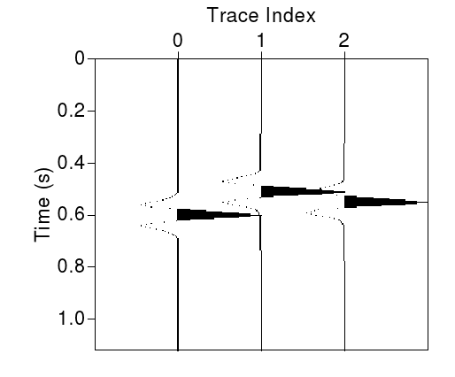
Figure 8: Three synthetic seismic traces that are shifted by random statics.

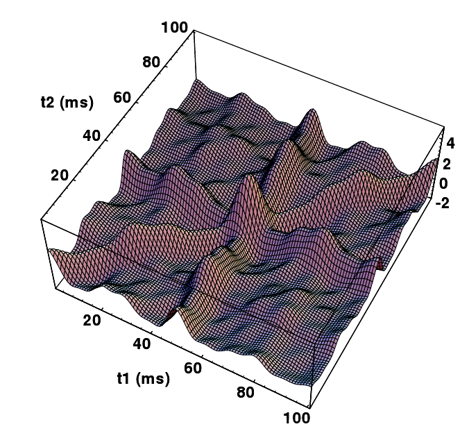
Figure 9: Landscape of a 2-D residual statics objective function.

Figure 9 shows a statics objective function with two unknowns. In practice, however, the time-shifts of the traces are not independent. The statics of each trace are caused by the combined time distortion of near-source and near-receiver heterogeneities (source-statics and receiver-statics). Figure 10 illustrates the similarity of travel paths near each source and each receiver.

Figure 10: A hypothetical model of the Earth’s upper crust showing rays associated with seismic waves propagating down from sources on the surface, reflecting off geologic boundaries and traveling upwards to receivers on the surface. Static-shifts of the seismic traces are caused by the combined time-distortions of near-source and near-receiver heterogeneities in the weathering layer.

The recorded reflection seismic signals are usually sorted into midpoints $y$ (of the source and receiver locations) and offsets $h$ (half distance between the source and receivers). Letting $\bf{s}$ and $\bf{r}$ be unknown vectors of source- and receiver-statics, this optimization problem can be formulated as

$$\max_{\bf{s},\bf{r}}F(\bf{s},\bf{r})=\sum_{y}{\sum_{h_{1}\neq h_{2}}{\Phi^{y}_{h_{1},h_{2}}(\tau(\bf{s},\bf{r}))}},$$ (25)

where $\Phi^{y}_{h_{1},h_{2}}(\tau)$ is the cross-correlation between traces (after a correction for propagation effects known as “normal move-out” has been applied) of offsets $h_{1}$ and $h_{2}$ at midpoint $y$ evaluated at

$$\tau=s_{i(y,h_{1})}+r_{j(y,h_{1})}-s_{i(y,h_{2})}-r_{j(y,h_{2})},$$

and $i(y,h)$ and $j(y,h)$ are the source and receiver indices for midpoint $y$ and offset $h$, respectively. The function $F(\bf{s},\bf{r})$ in equation (25) is called the stacking-power function.

Figure 11 shows the recording geometry of one example synthetic data set. This data set has $20$ sources, $35$ distinct receivers and $320$ traces. All traces are identical except for random source and receiver statics. These are generated by repeatedly shifting a single trace of field data. Thus, the objective function of equation (25) has $55$ unknowns. When there are no statics in the data, the global maximum of the function is at the origin (${\bf s}_{i}={\bf 0},\;{\bf r}_{j}={\bf 0}$). Figure 12 shows an arbitrary 2-D hyper-planes of the stacking-power function along the $10$th source and $20$ receiver statics.

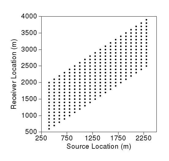
Figure 11: Recording geometry of a synthetic data set. The horizontal axis is the source position and vertical axis the receiver position.

We have analyzed a realistic synthetic statics problem involving some 320 seismic traces and 55 unknown static time shifts. A hyperplane through the objective function for this problem is shown in figure 12. In addition to simply computing the entropy of this function we will show how the entropy might be used to quantitatively address issues related to the topography of functions.

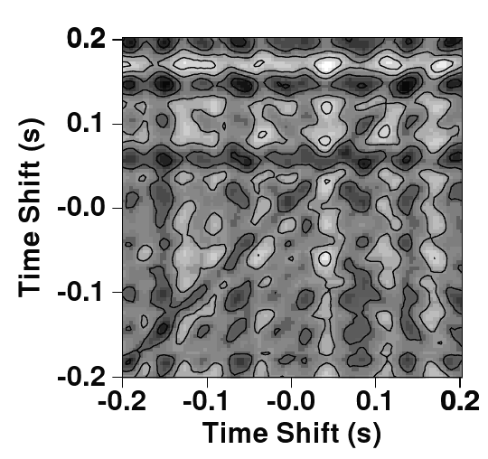
Figure 12: Hyperplane through the stacking-power function for a problem with 55 unknown static time shifts.

IV.2 Behavior of the Multi-Resolution Analysis

Rather than using Monte Carlo global optimization methods to solve the statics problem as in rothman85 ; rothman86 , Deng lydiawavelet has proposed, without proof, simplifying the optimization via a multi-resolution analysis (MRA) of the seismic traces. The idea is to use a wavelet decomposition to generate successively simpler representations of the seismic data, thereby eliminating progressively more local extrema from the objective function. To be precise, let us define a Multi-Resolution RHC algorithm:

Algorithm 3

MRHC $({\bf{\vec{m}}}={\mathit{M}RHC}(F,L,\epsilon,cmax))$
Let $\{{\bf S}_{i}\}_{i=L,\cdots,0}$ be a sequence of decreasingly smooth operators to be defined below, with ${\bf S}_{0}$ an identity operator.

1. Let $f_{L}={\bf S}_{L}\,F$; choose an initial population $\{{\bf m}^{0}_{k}\}_{k=1,\cdots,K}$ with size $K$ at random; apply Algorithm 2, so $\{{\bf m}_{k}\}_{k=1,\cdots,M_{L}}={\mathit{R}HC}(f_{L},K,\epsilon,cmax)$, and $i=L-1$.

2. Let $f_{i}={\bf S}_{i}\,F,\;(L>i\geq 0)$ and ${\bf{\vec{m}}}^{0}=\{{\bf m}_{k}\}_{k=1,\cdots,M_{i-1}}$; run Algorithm 2, $\{{\bf m}_{k}\}_{k=1,\cdots,M_{i}}={\mathit{R}HC}(f_{i},K,\epsilon,cmax)$.

3. Decrease the level index $i$ by $1$, repeat $2$ until $i=0$. The final set of models ${\bf{\vec{m}}}$ is the solution.

The smoothing operators $\{{\bf S}_{i}\}_{i=L,\cdots,0}$ could be a sequence of low-pass filters with increasingly wider pass-band bunks-saleck , or a sequence of increasingly fine wavelet operators lydiawavelet for decomposing the input seismic data. The sequence of smoothing operators should be such that the resulting functions, $\{f_{i}\}_{i=L,\cdots,0}$, have the same global feature as does the objective function $F$ for all levels and have decreasing number of local optima when the level increases, and $f_{0}=F$. Deng lydiawavelet showed that this could be achieved using the shift-invariant wavelet basis of Saito and Beylkin SA-BEY .

We now apply the entropy-based estimation of complexity to study the multi-resolution analysis of the 55 parameter statics problem introduced in the previous section. Figure 13 shows ${\hat{C}}_{e}$ as a function of the wavelet decomposition level using population $K=1000$; the mean and one-standard deviation error bars are obtained from 32 independent calculations. Results are shown for 6 levels of decomposition using a wavelet operator $\{{\bf S}\}_{i=0,...,5}$ where $i=0$ is an identity operator, corresponding to use of the original data. These results indicate that for this particular problem a complexity minimum is achieved for a wavelet decomposition of level 4. Higher levels of decomposition actually increase the complexity; presumably this results from the objective function being too flat for local optimization. Thus, the complexity measure gives us a way of choosing a wavelet decomposition level to achieve optimal simplification of an objective function.

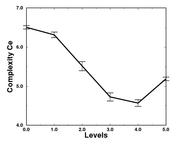
Figure 13: Complexity ${\hat{C}}_{e}$ as a function of the level of wavelet decomposition.

V Conclusions

We have developed a collection of simple tools for analysis of the topographic complexity of functions based on the application of local optimization to randomly chosen starting models. In particular we estimate the number of basins of attractions on the function landscape, the widths and depths of these basins and the entropy of the resulting probabilities.

Assuming local descent searches are ideal, we have computed the confidence intervals for the sampling error associated with this complexity measure. There are, on the other hand, several practical issues that we have neglected in this error analysis. Among them, we can mention the convergence error caused by the finite computing time and the finite precision of the local descent algorithms, the criterion for clustering of converged models, and the size of the assumed smallest basin of attraction, $p_{m}$. These issues can be investigated by a Monte Carlo analysis as shown in Figure 13.

VI Acknowledgments

This work is dedicated to the memory of Albert Tarantola. The authors thank Dr. Bill Navidi for useful discussions and comments on a draft of this work. This work was begun while the authors were at the Center for Wave Phenomena.

Appendix A Proofs of the Confidence Interval Analysis

A.1 Proof of Theorem1

Proof:

Let $K_{1},\dots,K_{n}$ be the random variables that represent the frequency of initial models converging to each local minima. The joint probability density for random variables $K_{i},\;i\in[1,n]$ for population of $K$ is a multinomial distribution. The marginal distribution for each of the random variables is,

$$f(k_{i})=\frac{K!}{k_{i}!(K-k_{i})!}p_{i}^{k_{i}}(1-p_{i})^{K-k_{i}},$$ (26)

and the corresponding statistical quantities are,

$$E[k_{i}]=K\,p_{i},\;\;\;\;var(k_{i})=Kp_{i}(1-p_{i}),$$

for $\forall i\in[1,n]$.

1. For $K$ such that $K\,p_{i}\geq 5$, the above binomial distribution can be approximated by a normal distribution. That is, the random variable,

   $$Z_{i} = \frac{k_{i}-Kp_{i}}{\sqrt{Kp_{i}(1-p_{i})}}$$

   $$= \frac{x_{i}-p_{i}}{\sqrt{p_{i}(1-p_{i})/K}}$$

   approaches to standard normal distributions $N(0,1)$ (Theorem 6.8 of freund ), where $x_{i}$ is defined in equation (7). Therefore, $x_{i}$ has a normal distribution with the mean and variance as in equations (18) and (19).

2. From equation (18), we see that $x_{i}$ is an unbiased estimator of $p_{i}$. Since $var(x_{i})\propto\frac{1}{K}$, we have

   $$\lim_{K\rightarrow\infty}var(x_{i})=0.$$ (27)

   Therefore,

   $$\lim_{K\rightarrow\infty}x_{i}=p_{i}.$$

   $x_{i}$ is also a consistent estimator of $p_{i}$ for each $i\in[1,n]$.

3. Now with confidence of $(1-\alpha)100\%$, we have

   $$|p_{i}-x_{i}|\leq\beta\sqrt{\frac{p_{i}\,(1-p_{i})}{K}},$$ (28)

   where the value of $\beta=z_{\alpha/2}$ can be looked up from a standard normal distribution table.

   However, we do not know $p_{i}$ in advance. Approximating $p_{i}$ by $x_{i}$ when $K$ is large, we have the confidence interval for the true $p_{i}$

   $$|p_{i}-x_{i}|\leq\beta\sqrt{\frac{x_{i}\,(1-x_{i})}{K}}$$ (29)

   for $i\in[1,n]$ (Theorem 11.6 of freund ).

$\Box$

A.2 Proof of Theorem 2

Proof:

From Theorem 1, we know that each random variable $x_{i}$ for $i\in[1,n]$ has an approximate normal distribution $N(p_{i},\frac{p_{i}\,(1-p_{i})}{K})$ when the population $K$ is such that $K\,p_{i}\geq 5$. Since ${\hat{q}}_{i}=cv_{i}x_{i}$, then ${\hat{q}}_{i}$ also has an approximate normal distribution $N(c\,v_{i}\,p_{i},\frac{c^{2}\,v^{2}_{i}\,p_{i}\,(1-p_{i})}{K})$. Since ${\hat{q}}_{i}$ would be very close to $q_{i}$ when $K$ is large, we can make the following approximation,

$${\hat{q}}_{i}\ln{\hat{q}}_{i}\approx q_{i}\ln q_{i}+(1+\ln q_{i})({\hat{q}}_{i}-q_{i}),$$ (30)

which is a linear function of the random variable ${\hat{q}}_{i}$. Therefore, ${\hat{q}}_{i}\ln{\hat{q}}_{i}$ is also approximate normal distribution,

$$E[{\hat{q}}_{i}\ln{\hat{q}}_{i}] = q_{i}\ln q_{i},$$ (31)

$$var({\hat{q}}_{i}\ln{\hat{q}}_{i}) = (1+\ln q_{i})^{2}\frac{c^{2}\,v^{2}_{i}\,p_{i}\,(1-p_{i})}{K}.$$ (32)

1. Since ${\hat{C}}_{e}$ is a linear combination of ${\hat{q}}_{i}\ln{\hat{q}}_{i}$ for $i\in[1,n]$, ${\hat{C}}_{e}$ also has an approximate normal distribution. Then, we have,

   $$E[{\hat{C}}_{e}]=-\sum_{i=1}^{n}E[{\hat{q}}_{i}\ln{\hat{q}}_{i}]=-\sum_{i=1}^{n}q_{i}\ln q_{i}=C_{e},$$

   and

   $$var({\hat{C}}_{e})=\sum_{i=1}^{n}var({\hat{q}}_{i}\ln{\hat{q}}_{i})+\sum_{i\neq j}Cov({\hat{q}}_{i}\ln{\hat{q}}_{i},{\hat{q}}_{j}\ln{\hat{q}}_{j}).$$

   For calculating $Cov({\hat{q}}_{i}\ln{\hat{q}}_{i},{\hat{q}}_{j}\ln{\hat{q}}_{j})$, recall equations (30) and (32),

   $$Cov({\hat{q}}_{i}\ln{\hat{q}}_{i},{\hat{q}}_{j}\ln{\hat{q}}_{j}) = E[({\hat{q}}_{i}\ln{\hat{q}}_{i}-q_{i}\ln q_{i})({\hat{q}}_{j}\ln{\hat{q}}_{j}-q_{j}\ln q_{j})]$$

   $$= (1+\ln q_{i})\,(1+\ln q_{j})Cov({\hat{q}}_{i},{\hat{q}}_{j})$$

   $$= (1+\ln q_{i})\,(1+\ln q_{j})c^{2}v_{i}\,v_{j}\,Cov(x_{i},x_{j}).$$

   We know that for a multinomial distribution,

   $$Cov(x_{i},x_{j})=-\frac{p_{i}\,p_{j}}{K}.$$ (33)

   Therefore,

   $$Cov({\hat{q}}_{i}\ln{\hat{q}}_{i},{\hat{q}}_{j}\ln{\hat{q}}_{j}) = -(1+\ln q_{i})\,(1+\ln q_{j})\,\frac{q_{i}\,q_{j}}{K}.$$ (34)

   So, the variance of ${\hat{C}}_{e}$ is

   $$var({\hat{C}}_{e}) = -\sum_{i=1}^{n}\sum_{j=1}^{n}\,(1+\ln q_{i})\,(1+\ln q_{j})\,\frac{q_{i}\,q_{j}}{K}$$

   $$+\sum_{i=1}^{n}(1+\ln q_{i})^{2}(\frac{c\,v_{i}\,q_{i}}{K}-\frac{q_{i}^{2}}{K})+\sum_{i=1}^{n}(1+\ln q_{i})^{2}\frac{q_{i}^{2}}{K}$$

   $$= -\sum_{i=1}^{n}\sum_{j=1}^{n}(1+\ln q_{i})\,(1+\ln q_{j})\,\frac{q_{i}\,q_{j}}{K}+\sum_{i=1}^{n}(1+\ln q_{i})^{2}\frac{c\,v_{i}\,q_{i}}{K}$$

   $$= -\frac{(1-C_{e})^{2}}{K}+\sum_{i=1}^{n}(1+\ln q_{i})^{2}\frac{c\,v_{i}\,q_{i}}{K}.$$

2. From equation (21), we see that this estimation is unbiased. Since $0<v_{i}\leq 1$ and $q_{i}$ is non-zero for each $i\in[1,n]$, and $var({\hat{C}}_{e})\propto\frac{1}{K}$ in equation (22), we can have

   $$\lim_{K\rightarrow\infty}var({\hat{C}}_{e})=0.$$

   Therefore, we have

   $$\lim_{K\rightarrow\infty}{\hat{C}}_{e}=C_{e},$$

   and hence ${\hat{C}}_{e}$ is a consistent estimator of $C_{e}$.

3. If the population size is large enough that $K\,p_{m}\geq 5$, then with confidence of $(1-\alpha)100\%$, the estimation error of the complexity ${\hat{C}}_{e}$ is at most $\beta\sigma_{{\hat{C}}_{e}}$, where $\sigma^{2}_{{\hat{C}}_{e}}=var({\hat{C}}_{e})$. That is,

   $$|{\hat{C}}_{e}-C_{e}| \leq \beta\,\sigma_{{\hat{C}}_{e}}.$$

   Replacing $p_{i}$ with the approximation $x_{i}$ in $\sigma_{{\hat{C}}_{e}}$ and considering $0<v_{i}\leq 1$, we have

   $$\sigma_{{\hat{C}}_{e}}^{2} \approx -\frac{(1-{\hat{C}}_{e})^{2}}{K}+\sum_{i=1}^{n}(1+\ln{\hat{q}}_{i})^{2}\frac{c\,v_{i}\,{\hat{q}}_{i}}{K}$$

   $$\leq -\frac{(1-{\hat{C}}_{e})^{2}}{K}+\frac{c}{K}\sum_{i=1}^{n}(1+\ln{\hat{q}}_{i})^{2}{\hat{q}}_{i}$$

   $$\leq -\frac{(1-{\hat{C}}_{e})^{2}}{K}+\frac{c}{K}(1-2{\hat{C}}_{e}-\ln{\hat{q}}_{min}{\hat{C}}_{e})$$

   $$= -\frac{(1-{\hat{C}}_{e})^{2}}{K}+\frac{c}{K}(1-(2+\ln{\hat{q}}_{min}){\hat{C}}_{e})=\delta^{2}.$$

   Since $\sigma_{{\hat{C}}_{e}}^{2}>0$, it is always true that $\delta^{2}\geq 0$. We have the third result of this theorem,

   $$|{\hat{C}}_{e}-C_{e}| \leq \beta\,\delta.$$

$\Box$

References

- (1) E.H.L. Aarts and Jan Korst. Simulated Annealing and Boltzman Machines. Wiley, N.Y, 1989.
- (2) O.M. Becker and M. Karplus. The topography of multidimensional potential energy surfaces: theory and application of peptide structure and kinetics. Journal of Physical Chemistry, 106:1495–1517, 1997.
- (3) R. S. Berry and R. Breitengraser-Kunz. Topography and dynamics of multidimensional interatomic potential surface. Physical Review Letters, 74:3951–3954, 1995.
- (4) C. Bunks, F. M. Saleck, S. Zaleski, and G. Chavent. Multiscale seismic waveform inversion. Geophysics, 60(5):1457–1473, September-October 1995.
- (5) G. Chavent. On the theory and practice of non-linear least-squares. Adv. Water Resources, 14:55–63, 1991.
- (6) T. E. Davis and J. C. Principe. A simulated annealing like convergence theory for the simple genetic algorithm. In R. K. Belew and L.B. Booker, editors, Proceedings of the fourth international conference on genetic algorithms. Morgan Kaufmann Publishers, San Mateo, Calif., 1991.
- (7) H. L. Deng. Using Multi-Resolution Analysis to study the complexity of inverse calculations. preprint, 1995.
- (8) H. L. Deng, W. Gouveia, and J. A. Scales. An object-oriented toolbox for studying optimization problems. In B. H. Jacobsen, K. Moosegard, and P. Sibani, editors, Inverse Methods, Interdisciplinary Elements of Methodology, Computation, and Applications, pages 320–330, Berlin, Germany, 1996. Springer-Verlag.
- (9) J. E. Dennis and R. B. Schnabel. Numerical methods for unconstrained optimization and nonlinear equations. Prentice-Hall Inc., 1987.
- (10) M. Falcioni, U. M. B. Marconi, P. M. Ginanneschi, and A. Vulpiani. Complexity of the minumum engery configurations. Physical Review Letters, 75:637–640, 1995.
- (11) R. Fletcher. Practical Methods of Optimization. John Wiley & Sons, 1987.
- (12) J. E. Freund. Mathematical Statistics. Prentice Hall, Englewood Cliffs, New Jersey, 5 edition, 1992.
- (13) D. E. Goldberg and M. P. Samtani. Engineering optimization via genetic algorithms. In Proceedings of the ninth conference on electronic computation, pages 471–482. 1986.
- (14) B. Hajek. Cooling schedules for optimal annealing. Mathematics of Operations Research, 13:311–329, 1988.
- (15) J. H. Holland. Adaptation in Natural and Artificial Systems. University of Michigan Press, Ann Harbor, MI, 1975.
- (16) S. A. Kauffman and E. D. Weinberger. The NK model of rugged fitness landscapes and its application to maturation of the immune response. Journal of Theoretical Biology, 141(2):211, 1989.
- (17) S. Kaufmann. The Origins of Order: Self-Organization and Selection in Evolution, chapter 2-3, pages 33–117. Oxford University Press, New York, 1993.
- (18) S. Kirkpatrick, C.D. Gelatt, and M.P. Vecchi. Optimization by simulated annealing. Science, 220:671–680, 1983.
- (19) D. H. Rothman. Nonlinear inversion, statistical mechanics, and residual statics estimation. Geophysics, 50:2797–2807, 1985.
- (20) D. H. Rothman. Nonlinear inversion, statistical mechanics, and residual statics estimation. Geophysics, 50:2797–2807, 1985.
- (21) D. H. Rothman. Automatic estimation of large residual statics corrections. Geophysics, 51:332–346, 1986.
- (22) N. Saito and G. Beylkin. Multiresolution representations using the auto-correlation functions of compactly supported wavelets. IEEE Transactions on Signal Processing, 41:3585–3590, 1993.
- (23) P. F. Stadler. Correlation in landscapes of combinatorial optimization problems. Europhysics Letters, 20(6):479–482, Nov 1992.
- (24) P. F. Stadler and R. Happel. Correlation structure of the landscape of the graph-bipartitioning problem. Journal of Physics. A, 25(11):3103–3110, June 1992.
- (25) P. F. Stadler and W. Schnabl. The landscape of the traveling salesman problem. Physics Letters A, 161:337–344, 1992.
- (26) A. A. Törn and A. Žilinskas. Global Optimization. Springer-Verlag, Berlin, Germany, 1989.
- (27) P.J.M. van Laarhoven and E.H.L. Aarts. Simulated Annealing: Theory and Practice. Reidel, Dordrecht, 1987.
- (28) David J. Wales and Janothon P. K. Doye. Global optimization by basin-hopping and the lowest energy structures of lennard-jones clusters containing up to 110 atoms. Journal of Physical Chemistry, pages 5111–5116, 1997.
- (29) David J. Wales, Mark A. Miller, and Tiffany R. Walsh. Archetypcal energy landscapes. Nature, 394:758–760, 1998.
- (30) E. D. Weinberger. Correlated and uncorrelated fitness landscapes and how to tell the difference. Biological Cybernetics, 63:325–336, 1990.
- (31) D. Whitley, K. Mathias, S. Rana, and J. Dzubera. Building better test functions. San Mateo, Calif., 1995. Morgan Kaufmann Publishers.