Wigner formalism for a particle on an infinite lattice: dynamics and spin

Abstract

The recently proposed Wigner function for a particle in an infinite lattice [NJP 14, 103009 (2012)] is extended here to include an internal degree of freedom, as spin. This extension is made by introducing a Wigner matrix. The formalism is developed to account for dynamical processes, with or without decoherence. We show explicit solutions for the case of Hamiltonian evolution under a position-dependent potential, and for evolution governed by a master equation under some simple models of decoherence, for which the Wigner matrix formalism is well suited. Discrete processes are also discussed. Finally we discuss the possibility of introducing a negativity concept for the Wigner function in the case in which the spin degree of freedom is included.

I Introduction

Since its introduction, the Wigner function (WF) PhysRev.40.749 has played an important role in physics. Quantum mechanics can be entirely formulated using this tool, therefore providing an alternative description of quantum phenomena, along with their dynamics. Also from a more experimental perspective, the WF has proven instrumental for tomographic reconstruction of the states prepared in the lab. The WF is in hence completely equivalent to the standard quantum mechanical formalism. Nevertheless, the particular features of the phase space description make it advantageous in some situations, for instance recognizing the quantum features of states, or dealing with decoherence scenarios. In the WF interference effects manifest in a clear way Lee2011 ; PhysRevA.74.042323 ; Hillery1984121 ; citeulike:4313181 . Another interesting property that manifests in the visualization of the WF of some states is the appearance of negative values over the phase space. This fact has been considered as a direct manifestation of the quantum nature of such states, and used to characterize their quantumness kenfack ; mari12 ; PhysRevLett.106.010403 . The relativistic extension of the Wigner function PhysRevD.13.950 has also found applications to a wide variety of problems, ranging from general relativistic kinetic theory and statistical mechanics nla.cat-vn1394639 ; Hakim:1379544 , nuclear matter at high densities and temperatures DiazAlonso:1991hy , electrons in magnetic fields Hakim1982 ; Yuan2010 , the quark-gluon plasma Elze1986 , to neutrino propagation in astrophysical or cosmological scenarios Sirera:1998ia ; YAMAMOTO2003 .

The applications mentioned above make use of a Wigner function defined in continuous space. It is nevertheless possible to introduce also a sensible Wigner function for systems on a discrete space. The definition for the case of a finite dimensional Hilbert space can be traced back to Stratonovich and Agarwal stratonovich ; PhysRevA.24.2889 (see also Varilly1989 ), who introduced a spherical, continuous phase space for a spin particle. A possible generalization was proposed by Wootters in 1987 Wootters1987 for prime dimensional systems, and later generalized to any power of primes in PhysRevA.70.062101 . A different construction was followed in leonhardt95prl ; PhysRevA.53.2998 ; miquel02qc which could cope with any dimension of the Hilbert space at the expense of enlarging the size of the phase space grid (see vourdas04review ; ferrie11review for a review). The discrete WF for a finite dimensional system is furthermore related to quantum information problems galvao05speedup ; ferrie11review ; Bianucci2002 ; miquel02qc ; PhysRevA.72.012309 ; veitch12 ; mari12 .

If the discrete Hilbert space is infinite dimensional, a different extension of the WF is required. In hinarejos12 we proposed a definition of the WF that can be used for such systems, having the correct marginal properties and with the advantage that a closed form can be obtain in some cases, such as the Gaussian states. Notice that, in contrast to the continuous case, where the axiomatic definition of the WF uniquely determines its functional form bertrand87 , in the discrete case different definitions are possible that respect the mathematical conditions enumerated above (see also PhysRevA.49.3255 ; rigas11 for alternative, related definitions, motivated by the study of the angle and angular momentum phase space).

Many of the problems where the continuous WF has found application concern particles with spin, or with spinor descriptions of quantum fields. In order to use the phase space formalism in this scenario, a generalization has to be introduced which combines the spin and spatial degrees of freedom (dof). One of the most common prescriptions in the literature is the use of a matrix valued WF PhysRevA.56.1205 , where the spinor or spin indices give rise to various matrix elements. Indeed, other possibilities exist, such as introducing a phase space for the spin degrees of freedom, which correspond to another discrete, finite dimensional Hilbert space, and construct a real valued WF for the cartesian product of spin and space phase spaces. In the matrix-valued WF, the treatment of space and spin dof is not symmetric. The spatial part is described in terms of a phase space, while the spin is unchanged. Although the treatment is asymmetric, such description has some advantages when dealing with a particle subject to a spin-dependent force, since some effects like the spin precession, or motion that depends on the spin component, are better visualized with respect to a fixed spin basis. Examples of this description are the analysis of the Stern-Gerlach experiment Utz2015 , the study of entangled vibronic quantum states of a trapped atom PhysRevA.56.1205 , or the reconstruction of the full entangled quantum state for the cyclotron and spin degrees of freedom of an electron in a Penning trap Massini2000 .

In this paper, we have extended the definition of the Wigner function introduced in hinarejos12 to incorporate the spin of a particle, using the Wigner matrix formalism for the spin degrees of freedom, and we illustrate the consequences of this definition by analyzing some simple physical situations, such as states involving spatial and spin entanglement or dynamical evolution, as it appears for a particle subject to a spin-dependent force.

The rest of this paper is organized as follows. In Section II we introduce a definition for the Wigner matrix (WM) that incorporates the spin of the particle, and summarize the main properties that are satisfied by this object. To illustrate the structure of this representation, we consider some simple cases in Section III. Section IV contains the main results of our paper, concerning the dynamics obeyed by the WM under the influence of an interacting Hamiltonian that may depend or not on the spin. First, we study the time evolution in continuous time, by deriving the equation of motion for the WM and solving this equation in some simple cases. The situation without spin serves us to consider the special case of a particle on a lattice interacting with a linear potential. We also investigate the interaction that appears for a spin-dependent force to visualize the main differences with the spinless case. Finally, we study the effect of decoherence for the system under consideration. Also in this Section, we show how one can make use of the WM to investigate the dynamics that appear in some discrete-time problems, and consider the particular example of the quantum walk. As before, we show the effect that decoherence may have on such problems.

One of the advantages of a WF description of continuous variable systems is the access to a negativity that measures the non-classicality of states. Although the relation of the negativity to non-classicality is well established, this quantity does not correspond to a physical observable. With a more general definition as the WM and the occurrence of (non-classical) spin degrees of freedom, we may wonder if there is a generalized negativity quantity and whether it retains some physical information. This is discussed in Section V. Section VI presents our main conclusions. The derivation of some formulae has been relegated to the Appendix in order to make our presentation more transparent.

II Particle with spin on a one-dimensional lattice

We are interested in the phase space description of a spin 1/2 particle that is allowed to move on an infinite 1D lattice. A paradigmatic example is the quantum walk (QW) on the line, where a particle moves along the sites of a 1D lattice. In its discrete-time version Aharonov93 , the direction of motion is dictated by the state of an extra two-dimensional Hilbert space (the coin), that can correspond to the internal spin of the moving particle. In fact, during the process the spatial and internal states become entangled, even if the initial state was separable, thus making clear the need for a joint description of both degrees of freedom. Another example is the study of spin dependent transport properties of single atoms in a 1D optical lattice Karski2011 .

We will start with the definition of the WF for a (spinless) particle on a 1D lattice already introduced in hinarejos12 . We consider a lattice with sites $\{na/n\in\mathbb{Z}\}$, where $a$ is the lattice spacing. To these sites one can associate a basis $\{\left|n\right\rangle$}, with $n\in\mathbb{Z}$. By a Fourier transformation we define a quasi-momentum basis, $|q\rangle=\sqrt{\frac{a}{2\pi}}\sum_{n}e^{iqna}|n\rangle$, which can be restricted to the first Brillouin zone, $q\in[-\frac{\pi}{a},\frac{\pi}{a}[$. The phase space is defined by points $(m,k)$, where $m\in\mathbb{Z}$, whereas $k$ is continuous and periodic, taking values in $[-\pi,\pi[$. With these notations, we define the WF as

$$W(m,k)\equiv\mathrm{tr}\left[\rho A(m,k)\right]=\frac{1}{2\pi}\sum_{n}\langle n|\rho|m-n\rangle e^{-i(2n-m)k},$$ (1)

where $\rho$ is the density operator corresponding to the state of the system, and $A(m,k)=\frac{1}{2\pi}\sum_{n}|m-n\rangle\langle n|e^{-i(2n-m)k}$ are the phase point operators for the lattice. It can be checked that the above definition fulfills the necessary requirements to be considered a valid WF. We refer the reader to the above reference for more information about the properties obeyed by (1).

We now would like to incorporate the additional degree of freedom arising from the spin of the particle. As discussed in the Introduction, there are different approaches in the literature to describe finite dimensional Hilbert spaces, such as the spin of a particle. One can combine both degrees of freedom (spin and lattice) by a tensor multiplication of the corresponding point operators, as done in Luis2005 for angular momentum and spin states.

As discussed in the introduction, here we opt for a prescription with ample acceptance in the continuous applications, namely a matrix-valued WF. A similar choice has been used in relativistic and non-relativistic setups with continuous spatial dof. Among the latter we can mention the study of Stern-Gerlach experiment Utz2015 , the analysis of entangled vibronic quantum states of a trapped atom PhysRevA.56.1205 , or the reconstruction of the full entangled quantum state for the cyclotron and spin degrees of freedom of an electron in a Penning trap Massini2000 . The Wigner function defined in this way combines the following properties:

- It keeps a close analogy with the definition of the relativistic Wigner function PhysRevD.13.950 ; nla.cat-vn1394639 ; Hakim:1379544 , thus allowing to describe the transition from the relativistic to the non relativistic regime.

- It appears as a simple and convenient choice to describe the spin motion in some particular cases, like the Stern-Gerlach experiment in continuous space Utz2015 , or the dynamics of a spin 1/2 particle on a lattice under the effect of a spin-dependent force, as described in Sect. IV.

We consider the Hilbert space $\mathcal{H}=\mathcal{H}_{l}\otimes\mathcal{H}_{s}$, where $\mathcal{H}_{l}$ stands for the motion on the lattice, and $\mathcal{H}_{s}$ describes the spin states. The composed Hilbert space is spanned by the basis $\{\left|n,\alpha\right\rangle\equiv\left|n\right\rangle\otimes\left|\alpha\right\rangle\}$ with $n\in\mathbb{Z}$ and $\left|\alpha\right\rangle/\alpha=0,1$ designate the eigenvectors of the $\sigma_{z}$ Pauli matrix (these states might also correspond to the computational basis of a qubit, or to the levels of a two level system). According to the above discussion, we propose the following definition for the WM

$$W_{\alpha\beta}(m,k)\equiv\frac{1}{2\pi}\sum_{n}\langle n,\alpha|\rho|m-n,\beta\rangle e^{-i(2n-m)k}.$$ (2)

We then have a set of four functions $W_{\alpha\beta}(m,k)$, $\alpha,\beta=0,1$ forming a $2\times 2$ matrix. Each function, as before, is defined on the phase space of points $(m,k)$, with $m\in\mathbb{Z}$, and $k$ takes values in $[-\pi,\pi[$. A similar definition can be made for any operator $\mathcal{O}$ acting on $\mathcal{H}$:

$$W_{\alpha\beta}^{\mathcal{O}}(m,k)\equiv\frac{1}{2\pi}\sum_{n}\langle n,\alpha|\mathcal{O}|m-n,\beta\rangle e^{-i(2n-m)k}.$$ (3)

Unlike the spatial variables, where the relationship with phase space points is non trivial, there is a direct correspondence between spin indices in the state of the system and indices in the matrix WF. This implies that operations on the spin space, such as rotations, change of basis or interactions with a spin-dependent force, as studied below, become more transparent using the matrix WF than other kind of representations for the spin. Moreover, the definition Eq. (2) keeps a closer analogy, for pure states, to the relativistic WF used in Quantum Field Theory. For such states one has $\rho=\left|\Psi\right\rangle\left\langle\Psi\right|$ and we can write

$$W_{\alpha\beta}(m,k)\equiv\frac{1}{2\pi}\sum_{n}\Psi_{\alpha}(n)\Psi_{\beta}^{*}(m-n)e^{-i(2n-m)k}$$ (4)

with $\Psi_{\alpha}(n)\equiv\langle n,\alpha\left|\Psi\right\rangle$. In the continuum limit, the functions $\Psi_{\alpha}(n)$ can be interpreted as the components of a Pauli spinor or a Dirac spinor. In this case, Eq. (4) can be related to the relativistic WF already mentioned in the Introduction.

Some of the properties discussed in hinarejos12 can be easily generalized for the matrix WF.

1) We have

$$W_{\beta\alpha}(m,k)=W_{\alpha\beta}^{*}(m,k),$$ (5)

which implies that the matrix WF is Hermitian. The normalization condition becomes

$$\sum_{\alpha}\sum_{m}\int_{-\pi}^{+\pi}dkW_{\alpha\alpha}(m,k)=1.$$ (6)

2) Also,

$$W_{\alpha\beta}(m,k\pm\pi)=(-1)^{m}W_{\alpha\beta}(m,k).$$ (7)

3) Given two operators $C$, $D$ and their corresponding Wigner matrices $W_{\alpha\beta}^{C}(m,k)$, $W_{\alpha\beta}^{D}(m,k)$ one has

$$2\pi\sum_{\alpha,\beta}\sum_{m=-\infty}^{\infty}\int_{-\pi}^{+\pi}dkW_{\alpha\beta}^{C}(m,k)W_{\beta\alpha}^{D}(m,k)=\mathrm{tr}\left(CD\right).$$ (8)

4) A complete knowledge of the WF can be used to reconstruct the density operator $\rho$:

$$\langle\alpha|\rho|\beta\rangle=2\pi\sum_{m}\int_{-\pi}^{+\pi}dkW_{\alpha\beta}(m,k)A(m,k).$$ (9)

5) The marginal distributions of (2) are related to matrix elements of the density operator

$$\sum_{m=-\infty}^{+\infty}W_{\alpha\beta}(m,k)=\tfrac{1}{a}\langle\tfrac{k}{a},\alpha|\rho|\tfrac{k}{a},\beta\rangle,$$ (10)

and

$$\int_{-\pi}^{+\pi}dkW_{\alpha\beta}(m,k)=\sum_{n}\delta_{m,2n}\langle n,\alpha|\rho|n,\beta\rangle.$$ (11)

As already discussed in hinarejos12 , these equations reflect the distinction between the coordinates of the phase space points, $m\in\mathbb{Z}$, $k\in[-\pi,\pi[$, and the position and quasimomentum bases, $n,$ $q$. The $k$ coordinate is adimensional and does not directly represent a momentum value, but is connected to $q=k/a$. The spatial label $m$ in phase-space is only connected to a discrete position, $s$, for even values, $m=2s$, while the odd values of $m$ are analogous to the odd half-integer phase space grid points in PhysRevA.53.2998 ; miquel02qc .

III Particular cases

In order to obtain some insight about the characteristics of the matrix WF Eq. (2), we will give the explicit form it takes for some particular cases.

• Product state

We start by considering a product state of spatial and spin degrees of freedom

$$\rho=\rho_{L}\otimes\rho_{S},$$ (12)

where $\rho_{L}$ represents a general state on the lattice, and $\rho_{S}$ is an arbitrary spin state. In this case, we readily obtain

$$W_{\alpha\beta}(m,k)=W_{L}(m,k)\langle\alpha|\rho_{S}|\beta\rangle,$$ (13)

with

$$W_{L}(m,k)\equiv\frac{1}{2\pi}\sum_{n}\langle n|\rho_{L}|m-n\rangle e^{-i(2n-m)k}.$$ (14)

• Superposition of two deltas

Let us consider the WM for the state formed by a superposition of two localized states at lattice sites $\left|n_{1}\right\rangle$ and $\left|n_{2}\right\rangle$ with $n_{1}\neq n_{2}\in\mathbb{Z}$

$$\mid\Psi_{2\delta}\rangle=\frac{1}{\sqrt{1+\mid\alpha\mid^{2}}}(\left|n_{1}\right\rangle\mid 0\rangle+\alpha\left|n_{2}\right\rangle\mid 1\rangle),$$ (15)

where $\alpha$ is an arbitrary complex number that represents the relative weight of the state $\left|n_{2}\right\rangle$. For $\alpha=1$ we obtain a Schrödinger-cat state. The corresponding WF can be easily calculated. Written in matrix form in the above spin basis,

$$W(m,k)=\frac{1}{2\pi(1+\mid\alpha\mid^{2})}\left(\begin{array}[]{ccc}\delta_{m,2n_{1}}&\alpha^{*}e^{-ik(n_{1}-n_{2})}\delta_{m,n_{1}+n_{2}}\\ \alpha e^{ik(n_{1}-n_{2})}\delta_{m,n_{1}+n_{2}}&\mid\alpha\mid^{2}\delta_{m,2n_{2}}\end{array}\right)$$ (16)

In this case, the WM is zero everywhere except for three particular values of the space-like phase coordinate, $m=2n_{1},2n_{2},n_{1}+n_{2}$. It is interesting to compare the structure provided by Eq. (16) with the corresponding superposition of two localized states without spin hinarejos12 , given by

$$\mid\Psi_{2\delta}^{no\,spin}\rangle=\frac{1}{\sqrt{1+\mid\alpha\mid^{2}}}(\left|n_{1}\right\rangle+\alpha\left|n_{2}\right\rangle).$$ (17)

In that case, the WF is a scalar function

$$W_{2\delta}^{no\,spin}(m,k) = \frac{1}{2\pi(1+|\alpha|^{2})}\left\{\delta_{m,2n_{1}}+|\alpha|^{2}\delta_{m,2n_{2}}\right.$$ (18)

$$\quad\left.+2|\alpha|\delta_{m,n_{1}+n_{2}}\cos[\Delta n\ k+\phi]\right\},$$

where $\phi$ is the phase of the complex coefficient $\alpha$, and $\Delta n=n_{2}-n_{1}$. One observes the different terms in (18) appear distributed on different matrix positions in Eq. (16). In particular, the out of diagonal term in (16) corresponds to the interference, oscillating term in (18). This term plays an interesting role related to the non positivity of the WF. We will return to this point later.

• Superposition of two Gaussian states

The superposition of two discretized pure Gaussian states with orthogonal spin components is another interesting state for which the WM defined in this work can be computed analytically. Such a state is defined as

$$|\Psi_{2G}\rangle=\frac{1}{\sqrt{2}{\cal N}}\sum_{n}\left\{e^{-\frac{(n-a)^{2}}{2\sigma^{2}}}\mid 0\rangle+e^{-\frac{(n-b)^{2}}{2\sigma^{2}}}\mid 1\rangle\right\}|n\rangle,$$ (19)

for arbitrary $a,b\in\mathbb{Z}$, $\sigma\in\mathbb{R}^{+}$. For this state, the WF can be expressed as a matrix in the same $\{\left|0\right\rangle,\left|1\right\rangle\}$ basis

$$W(m,k)=\frac{1}{2}\left(\begin{array}[]{ccc}W_{a}(m,k)&W_{ab}(m,k)\\ W_{ab}^{*}(m,k)&W_{b}(m,k)\end{array}\right)$$ (20)

where

$$W_{l}(m,k)=\frac{1}{2\pi{\cal N}^{2}}e^{-\frac{l^{2}+(m-l)^{2}}{2\sigma^{2}}}e^{ikm}\theta_{3}(k+\frac{im}{2\sigma^{2}},e^{-\frac{1}{\sigma^{2}}}),\,\,\,l=a,b$$ (21)

$$W_{ab}(m,k)=\frac{1}{2\pi{\cal N}^{2}}e^{-\frac{a^{2}+(m-b)^{2}}{2\sigma^{2}}}e^{ikm}\theta_{3}(k+\frac{i(m-b+a)}{2\sigma^{2}},e^{-\frac{1}{\sigma^{2}}})$$ (22)

with ${\cal N}=\sqrt{\theta_{3}(0,e^{-\frac{1}{\sigma^{2}}})}$ the normalization constant. The Jacobi theta function $\theta_{3}(z,q)$ is defined as $\theta_{3}(z,q)\equiv\sum_{n}q^{n^{2}}e^{2izn}$ for complex arguments $q$, $z$, with $|q|<1$ abramsteg . As in the previous example, we find an important difference with the WF for the case without spin hinarejos12 , since the components in the scalar function appear here distributed as the components of the matrix WF. In the limit $a=-b\gg\sigma$ with $\sigma\rightarrow 0$ we recover the result for the two deltas (16) corresponding to the case $n_{1}=-n_{2}=a$ and $\alpha=1$.

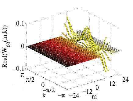
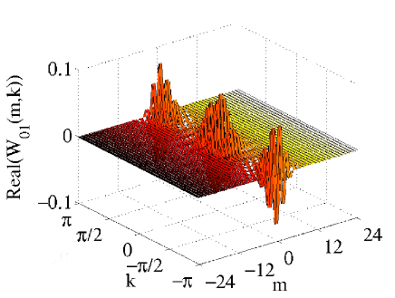
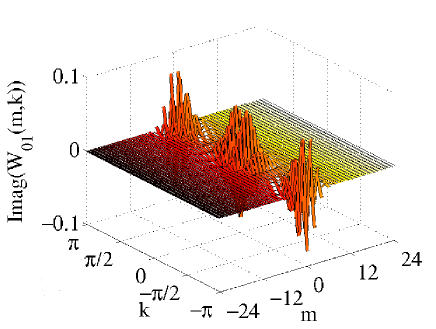
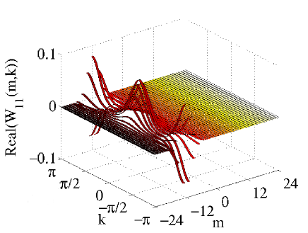
Figure 1: Matrix components of the WM for two Gaussians, as given by Eqs. (20-22). Panel a) represents $W_{a}(m,k)$, panel b) is the real part of $W_{ab}(m,k)$, while the imaginary part is plotted on panel c). Finally, panel d) shows the $W_{b}(m,k)$ component. In these plots, $a=-b=6$ and $\sigma=1.5$.

Figure 1 shows the four components of the WM for a two-Gaussian state, as given by Eqs. (20-22). One can immediately observe on each component the presence of a secondary image that reflects the property Eq. (7). In hinarejos12 we discussed with some detail, for the spinless case, the peculiarities related to this duplicate.

IV Dynamics

The WF formalism can be used, not only to allow for a description of a given state, but also to analyze the dynamics, and to visualize it in phase space. Our purpose is to study the motion of a particle on a lattice in terms of the corresponding WF. We start from the simplest case, which corresponds to the spinless particle, and then move to a more general situation, where the particle interacts with a spin-dependent term. The time evolution will be first considered within continuous time, a situation that can be applied to most problems in physics, and can be described by the Schrödinger equation.

IV.1 Continuous time

IV.1.1 Particle without spin

Let us consider a spinless particle moving on a lattice under the influence of a potential $V$ that depends on the lattice site. We concentrate on the following Hamiltonian

$$H=J(T_{+}+T_{-})+V,$$ (23)

that appears as a consequence of the tight-binding approximation in crystals, where the parameter $J$ is a characteristic of the system which is related to the hopping probability of an electron to the nearest neighbor, and the displacement operators $T_{\pm}$ are defined by $T_{\pm}\left|n\right\rangle=\left|n\pm 1\right\rangle$. Notice that the Hamiltonian (23) can also be considered as a discretized version of

$$H_{cont}=-\frac{\nabla^{2}}{2M}+V(x)$$ (24)

(with $M$ the mass of the particle) if one defines $J=-\frac{1}{2Ma^{2}}$.

The wave function can be written as $\psi(n,t)$, with $t$ the time, so that the Schrödinger equation reads

$$i\frac{\partial}{\partial t}\psi(n,t)=J\left[\psi(n+1,t)+\psi(n-1,t)-2\psi(n,t)\right]+V_{n}\psi(n,t),$$ (25)

with $V_{n}\equiv\langle n|V|n\rangle$. The last term inside the brackets in Eq. (1) can be easily reabsorbed into the definition of the coefficients $V_{n}$ (it can be also understood as a term proportional to the identity in the Hamiltonian, thus contributing only as a position-independent phase as time evolves). Therefore we omit that term.

It is straightforward to derive an evolution equation satisfied by the WF for the above problem. We begin with the von Neumann equation for the density operator

$$\frac{\partial}{\partial t}\rho(t)=-i[H,\rho(t)].$$ (26)

Making use of (1) one arrives to

$$\frac{\partial}{\partial t}W(m,k,t)=2J\sin k\left[W(m+1,k,t)-W(m-1,k,t)\right]-\frac{i}{2\pi}\sum_{l}e^{-i(2l-m)k}(V_{l}-V_{m-l})\langle l|\rho(t)|m-l\rangle,$$ (27)

where we have explicitly showed the time dependence of $\rho$ and $W(m,k)$ for the sake of clarity.

Let us consider that $V(x)$ is a continuous and infinitely derivable function. In this case, one can obtain a closed form of the above expression for the WF, as showed in the Appendix. As a result, one arrives to the following expression

$$\frac{\partial}{\partial t}W(m,k,t)=2J\sin k\left[W(m+1,k,t)-W(m-1,k,t)\right]+\sum_{s=0}^{\infty}\frac{(-1)^{s}a^{2s+1}}{2^{2s}(2s+1)!}\left.\frac{d^{2s+1}V(x)}{dx^{2s+1}}\right|{}_{x=ma/2}\frac{\partial^{2s+1}W(m,k,t)}{\partial k^{2s+1}}.$$ (28)

It must be noticed that Eq. (28) also holds for the WM (2) if we introduce the spin of the particle, by simply replacing $W(m,k,t)\longrightarrow W_{\alpha\beta}(m,k,t)$, since none of the spatial operations in this equation can affect the spin indices.

Before we go on, we will consider the continuous limit ($a\to 0$) of Eq. (28). In this limit, our WF has to be replaced by the corresponding function $W_{\mathrm{c}}(x,q,t)$ following the prescription hinarejos12

$$W(m,k,t)\underset{a\to 0}{\longrightarrow}\frac{1}{2}W_{\mathrm{c}}(x=\frac{ma}{2},q=\frac{k}{a},t).$$ (29)

By replacing $J=-\frac{1}{2Ma^{2}}$ and substituting (29) in (28), and taking the limit ($a\to 0$), one obtains the equation

$$\frac{\partial}{\partial t}W_{c}(x,q,t)+\frac{q}{M}\frac{\partial}{\partial x}W_{c}(x,q,t)=\sum_{s=0}^{\infty}\frac{(-1)^{s}}{2^{2s}(2s+1)!}\left.\frac{d^{2s+1}V(x)}{dx^{2s+1}}\right|{}_{x=ma/2}\frac{\partial^{2s+1}W_{c}(x,q,t)}{\partial q^{2s+1}}.$$ (30)

Eq. (30) is the equation of motion for the WF under the effect of an external potential $V(x)$ in continuous space, where $q$ represents the momentum of the particle (ranging from $-\infty$ to $\infty$) (see, for example Hillery1984121 ).

As an interesting particular case, we will study the case of a linear potential, i.e. $V(x)=\lambda x$, with $\lambda$ a real constant. Eq. (28) adopts a simple form

$$\frac{\partial}{\partial t}W(m,k,t)=2J\sin k\left[W(m+1,k,t)-W(m-1,k,t)\right]+\lambda a\frac{\partial}{\partial k}W(m,k,t).$$ (31)

To solve this equation, we perform a Fourier transformation on the variable $m$ by introducing the function

$$\tilde{W}(q,k,t)\equiv\frac{1}{\sqrt{2\pi}}\sum_{m}e^{iqm}W(m,k,t),$$ (32)

the new variable $q$ taking values on the interval $[-\pi,\pi[$. With the help of this function, we can rewrite Eq. (32) as

$$\frac{\partial}{\partial t}\tilde{W}(q,k,t)=-4iJ\sin k\sin q\tilde{W}(q,k,t)+\lambda a\frac{\partial}{\partial k}\tilde{W}(q,k,t).$$ (33)

The change of function

$$\tilde{W}(q,k,t)\equiv e^{-\frac{4iJ\cos k\sin q}{\lambda a}}f(q,k,t)$$ (34)

leads to the following equation for $f(q,k,t)$:

$$\frac{\partial}{\partial t}f(q,k,t)=\lambda a\frac{\partial}{\partial k}f(q,k,t),$$ (35)

which implies that $f(q,k,t)$ must be of the form $f(q,k,t)=g(q,k+\lambda at),$ with $g(q,k)$ an unknown function that can be determined by the initial ($t=0$) condition in Eq. (34), giving

$$g(q,k)=e^{\frac{4iJ\cos k\sin q}{\lambda a}}\tilde{W}(q,k,0).$$ (36)

We finally obtain, after some algebra

$$\tilde{W}(q,k,t)=\exp[-8i\frac{J}{\lambda a}\sin(k+\frac{\lambda at}{2})\sin(\frac{\lambda at}{2})\sin q]\tilde{W}(q,k+\lambda at,0).$$ (37)

To derive an expression for the WF, we need the inverse relation of Eq. (32), given by

$$W(m,k,t)=\frac{1}{\sqrt{2\pi}}\int_{-\pi}^{\pi}dqe^{-iqm}\tilde{W}(q,k,t),$$ (38)

and make use of the formula gradshteyn2007

$$J_{n}(z)=\frac{1}{2\pi}\int_{-\pi}^{\pi}dqe^{-inq}e^{iz\sin q},$$ (39)

where $n\in\mathbb{Z}$, $z\in\mathbb{C}$, and $J_{n}(z)$ are the Bessel functions of the first kind. After substituting Eq. (37) into (38) we arrive to the final expression

$$W(m,k,t)=\sum_{l}J_{m-l}\left[-8\frac{J}{\lambda a}\sin(k+\frac{\lambda at}{2})\sin\frac{\lambda at}{2}\right]W(l,k+\lambda at,0).$$ (40)

Notice that, in the latter equation, the argument $k+\lambda at$ is to be understood modulo $2\pi$. Using this fact, one can readily obtain that the above solution exhibits a time periodicity

$$W(m,k,t+\frac{2\pi}{\lambda a})=W(m,k,t),$$ (41)

which corresponds to the well known phenomenon of Bloch oscillations, that can be observed for electrons confined in a periodic potential (the lattice) subject to a constant force, as for example a constant electric field. The corresponding frequency $\omega_{B}=\left|\lambda\right|a$ is precisely what is expected for our linear potential $V(x)=\lambda x$.

Directly related to the above treatment, it appears quite natural to attempt a parallelism with a situation that describes the dynamics of a particle under the effect of a constant gravitational field, $V(x)=m_{g}gx$, where $m_{g}$ is the gravitational mass and $g$ the acceleration of gravity. Notice that, for the following discussion to make sense, one should design a physical system that is described by this potential, and that Eq. (25) can be considered as a discretized approximation to (24), with $J=-\frac{1}{2Ma^{2}}$ . We will return to this discussion later.

We find it convenient to use the symbol $m_{i}$ instead of $M$ to represent the inertial mass, and to recover the Planck constant. We observe that the argument of the Bessel functions in Eq. (40) depends upon the combination

$$-\frac{J}{\lambda a}=\frac{\hbar^{2}}{2m_{i}m_{g}ga^{3}}\equiv\frac{1}{(k_{g}a)^{3}},$$ (42)

where $k_{g}\equiv(\frac{2m_{i}m_{g}g}{\hbar^{2}})^{1/3}$ is a characteristic wave vector that modulates the spatial dependence of energy eigenstates in a gravitational field in continuous space kajari2010 . As the authors of this work discuss, this is one of the possible effects for quantum particles under the effect of gravity, where various combinations of (powers of) $m_{g}$ and $m_{i}$ may appear depending on the problem under consideration, thus paving the way to measuring these two quantities independently.

The dynamics on the lattice we just considered offers a similar perspective. The time evolution in Eq. (40) is governed by the product $k_{g}a$, which involves the lattice spacing as a new parameter, thus allowing an extra degree of freedom in the design of experiments, if they are performed on a lattice instead of in continuous space. However, one has to be careful about this point: Only if the design of the experiment is such that $J$ and $V(x)$ correspond to the above hypothesis, the previous discussion can make sense.

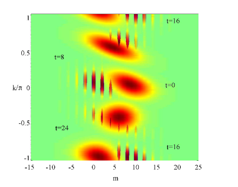
Figure 2: Snapshots corresponding to the time evolution of the WF, as given by Eq. (40) with an initial Gaussian state of the form (21) with $a=3$ and $\sigma=2$. The parameters of the Hamiltonian are $J=1$ and $\lambda a=1$. The labels indicate different values of time.

To illustrate the behavior of the WF, we plotted in Fig. 2 several snapshots obtained by evolving an initial Gaussian state of the form (21). The time evolution is governed by Eq. (40). One observes several features on this plot. First, the position of the maximum shows oscillations for the variable $m$, as corresponding to the Bloch oscillations discussed above, while variable $k$ evolves linearly (and periodically) with time. During the evolution, the WF also experiences a distortion that is similar to the one observed in continuous space kajari2010 . One also observes the presence of a secondary image which manifests as vertical strips.

IV.1.2 Particle with spin

We return to the description of a particle with spin 1/2. Our purpose is to analyze the dynamics for such a system, and compare it with the spinless case. To do so, we need to introduce some spin-dependent potential, otherwise the different components in the WM will evolve exactly in the same way, and the results of the previous subsection apply. In order to make this comparison as close as possible, we will consider the time evolution under the effect of a Hamiltonian of the form

$$H=J(T_{+}+T_{-})+\sigma_{z}V,$$ (43)

where $V$ is, as before, a site-dependent scalar potential. It is possible to obtain an evolution equation, similar to (28), when the particle is subject to the above Hamiltonian in the lattice. This derivation is made in the Appendix, the main difference with the spinless case being that the diagonal and off-diagonal components of the WM evolve differently. In what follows, we concentrate on the particular example of a discretized linear potential $V_{n}=\lambda an$, with $\lambda$ a real constant. Then, Eq. (72) particularizes to

$$\frac{\partial}{\partial t}W_{\alpha\alpha}(m,k,t)=2J\sin k\left[W_{\alpha\alpha}(m+1,k,t)-W_{\alpha\alpha}(m-1,k,t)\right]+(-1)^{\alpha}\lambda a\frac{\partial}{\partial k}W_{\alpha\alpha}(m,k,t),$$ (44)

and

$$\frac{\partial}{\partial t}W_{\alpha\beta}(m,k,t)=2J\sin k\left[W_{\alpha\beta}(m+1,k,t)-W_{\alpha\beta}(m-1,k,t)\right]-i(-1)^{\alpha}\lambda amW_{\alpha\beta}(m,k,t),$$ (45)

(valid for $\alpha\neq\beta$).

The first equation can be easily solved by comparison to (31). We only have to perform the replacement $\lambda\longrightarrow(-1)^{\alpha}\lambda$. Therefore, we can write the solution using the same procedure as in the case with no spin, to obtain

$$W_{\alpha\alpha}(m,k,t)=\sum_{l}J_{m-l}\left[-8\frac{J}{\lambda a}\sin(k+(-1)^{\alpha}\frac{\lambda at}{2})\sin\frac{\lambda at}{2}\right]W_{\alpha\alpha}(l,k+(-1)^{\alpha}\lambda at,0).$$ (46)

The same comments made in the previous section hold here: $W_{\alpha\alpha}(m,k,t)$ is periodic in time, with frequency given by $\omega_{B}=\left|\lambda\right|a$ . Eq. (45) can be solved by introducing a Fourier transform, as made with (31). We arrive, after some algebra, at

$$W_{\alpha\beta}(m,k,t)=e^{(-1)^{\alpha}im\frac{\lambda at}{2}}\sum_{l}e^{(-1)^{\alpha}il\frac{\lambda at}{2}}J_{m-l}\left[-8\frac{J}{\lambda a}\sin k\sin\frac{\lambda at}{2}\right]W_{\alpha\beta}(l,k,0).$$ (47)

(valid when $\alpha\neq\beta$).

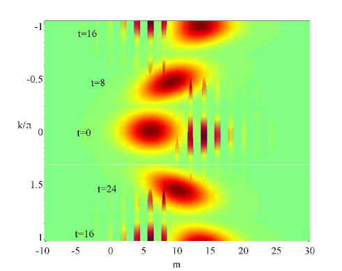
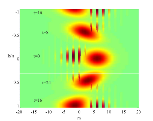
Figure 3: The two panels show the diagonal components of the WM at four different times (labeled by the corresponding $t$), for a particle subject to the interaction Hamiltonian (43) in a lattice. Left panel corresponds to $W_{00}(m,k,t)$, whereas right panel shows $W_{11}(m,k,t)$. The initial state is a separable state (see the main text for explanation) with $a=3$, $\sigma=2$. The parameters of the interaction Hamiltonian are $J=\lambda a=1$.

To illustrate the evolution of the WM elements under the effect of the Hamiltonian (43) with a linear potential, we followed this evolution for an initial separable state of the form (13), with $\rho_{S}$ defined by the pure state $\frac{1}{\sqrt{2}}(\left|0\right\rangle+\left|1\right\rangle)$ and $W_{L}(m,k)$ corresponding to a Gaussian state, given by (c.f. Eq. (21))

$$W_{L}(m,k)=\frac{1}{2\pi{\cal N}^{2}}e^{-\frac{a^{2}+(m-a)^{2}}{2\sigma^{2}}}e^{ikm}\theta_{3}(k+\frac{im}{2\sigma^{2}},e^{-\frac{1}{\sigma^{2}}})$$ (48)

and ${\cal N}=\sqrt{\theta_{3}(0,e^{-\frac{1}{\sigma^{2}})}}$ the normalization constant. The results are presented in Fig. 3, which shows different snapshots of the diagonal components $W_{00}(m,k,t)$ and $W_{11}(m,k,t)$ of the WM. We observe that both components present similar features to the case without spin, plotted in Fig. 2. However, they evolve differently on the $m$ axis: Initially, the $W_{00}(m,k,t)$ component moves to the left, while the $W_{11}(m,k,t)$ component moves to the right, as a consequence of the different time dependence $(-1)^{\alpha}\lambda at$ in (46), a phenomenon which is reminiscent of the splitting into two beams on the Stern-Gerlach experiment, where the basic piece of the interaction is analogous to (43).

IV.1.3 Decoherence

Another dynamical scenario of great relevance for the study of quantum systems is the presence of decoherence, which can be caused by interaction with the environment. In the following we show how the WF formalism we are discussing accommodates also such situation. In particular, we explore some typical cases, in which the spin structure of the WM allows a simple visualization of the decoherence effects.

We consider the case where the interaction with the environment can be described by a Lindblad-type equation Breuer2007

$$\frac{\partial}{\partial t}\rho=-i[H,\rho]+\sum_{k}\gamma_{k}(A_{k}\rho A_{k}^{\dagger}-\frac{1}{2}A_{k}^{\dagger}A_{k}\rho-\frac{1}{2}\rho A_{k}^{\dagger}A_{k}),$$ (49)

where $A_{k}$ are the Lindblad operators, and $\gamma_{k}$ represent the corresponding coupling constants.

If these operators act only on the spin space, the Lindblad (noise) term Eq. (49) immediate translates in an analogous equation for the WM. In other words, under this hypothesis we can write for the WM

$$\frac{\partial}{\partial t}W(m,k,t)=\frac{\partial}{\partial t}W(m,k,t)|_{H}+\sum_{k}\gamma_{k}(A_{k}W(m,k,t)A_{k}^{\dagger}-\frac{1}{2}A_{k}^{\dagger}A_{k}W(m,k,t)-\frac{1}{2}W(m,k,t)A_{k}^{\dagger}A_{k}).$$ (50)

In the latter equation, $\frac{\partial}{\partial t}W(m,k,t)|_{H}$ denotes the contribution of the Hamiltonian to the dynamics (without decoherence), and we used a matrix notation, so that spin indices are omitted.

As a simple example, let us consider the case when we only have a Lindblad operator $A_{1}=\sigma_{z}$ with $\gamma_{1}\equiv\gamma$. We then have

$$\frac{\partial}{\partial t}W(m,k,t)=\frac{\partial}{\partial t}W(m,k,t)|_{H}+\left(\begin{array}[]{cc}0&-2\gamma W_{01}(m,k,t)\\ -2\gamma W_{10}(m,k,t)&0\end{array}\right),$$ (51)

which solution can be readily obtained, and expressed as

$$W(m,k,t)=\left(\begin{array}[]{cc}W_{00}(m,k,t)|_{H}&e^{-2\gamma t}W_{01}(m,k,t)|_{H}\\ e^{-2\gamma t}W_{10}(m,k,t)|_{H}&W_{11}(m,k,t)|_{H}\end{array}\right).$$ (52)

In other words, in this example decoherence leaves the diagonal terms unaltered, while the off-diagonal terms are exponentially damped with time.

Our second example is provided by the Lindblad operator $A_{1}=\sigma_{x}$ with $\gamma_{1}\equiv\gamma$. In this case, Eq. (50) becomes

$$\frac{\partial}{\partial t}W(m,k,t)=\frac{\partial}{\partial t}W(m,k,t)|_{H}+\gamma\left(\begin{array}[]{cc}W_{11}(m,k,t)-W_{00}(m,k,t)&W_{10}(m,k,t)-W_{01}(m,k,t)\\ W_{01}(m,k,t)-W_{10}(m,k,t)&W_{00}(m,k,t)-W_{11}(m,k,t)\end{array}\right).$$ (53)

This set of equations can be solved by elementary operations. We concentrate on the diagonal terms, for which the final solution reads

$$W_{00}(m,k,t)=\frac{1}{2}(1+e^{-2\gamma t})W_{00}(m,k,t)|_{H}+\frac{1}{2}(1-e^{-2\gamma t})W_{11}(m,k,t)|_{H},$$ (54)

$$W_{11}(m,k,t)=\frac{1}{2}(1-e^{-2\gamma t})W_{00}(m,k,t)|_{H}+\frac{1}{2}(1+e^{-2\gamma t})W_{11}(m,k,t)|_{H}.$$ (55)

Similar equations can be obtained involving $W_{01}(m,k,t)$ and $W_{10}(m,k,t)$. As a result, in the limit $t\longrightarrow\infty$ both $W_{00}(m,k,t)$ and $W_{11}(m,k,t)$ become an equally weighted mixture (the same happens with the off-diagonal terms).

IV.2 Discrete time

IV.2.1 Quantum walk

The examples studied in the previous Section arise as a consequence of the continuous interaction of a particle with an external potential acting on the lattice. However, we can envisage some situations in which we act on the particle with subsequent short pulses, or via some actions that appear suddenly, but regularly in time. A paradigmatic example of this kind is provided by the quantum walk Aharonov93 ; Venegas-Andrac2012 , which has received a lot of interest in recent years. In the discrete quantum walk, a quantum particle moves on an (1D) lattice subject to the periodic influence of a displacement operator, that propagates the particle to the right or to the left, according to the state of a two-level system (the coin). The total Hilbert space has precisely the structure $\mathcal{H}=\mathcal{H}_{l}\otimes\mathcal{H}_{s}$, defined in Sect. II and, in fact, we can associate the states of the coin to the spin of the particle, without loss of generality. It is customary to use the basis states $\left|L\right\rangle$ and $\left|R\right\rangle$ in $\mathcal{H}_{s}$ (instead of $\left|0\right\rangle$ and $\left|1\right\rangle$) and associate them to the left and right propagation, respectively. We consider the successive application of the unitary transformation

$$U(\theta)=\left\{T_{-}\otimes|L\rangle\langle L|+T_{+}\otimes|R\rangle\langle R|\right\}\otimes C(\theta),$$ (56)

where $C(\theta)=I\otimes\sigma_{z}e^{-i\theta\sigma_{y}}$, $\theta\in\left[0,\pi/2\right]$ is a parameter defining the bias of the coin toss, $I$ is the identity operator in $\mathcal{H}_{l}$, and $\sigma_{y}$ and $\sigma_{z}$ are Pauli matrices acting on $\mathcal{H}_{s}$. The QW dynamics can be described entirely in terms of the WM Hinarejos2013 , via a recursion formula that relates $W(m,k,t+1)$ to other components of this function at time $t$. Using Eq. (56) one obtains, after some algebra:

$$W(m,k,t+1) =M_{R}W(m-2,k,t)M_{R}^{\dagger}+e^{-2ik}M_{R}W(m,k,t)M_{L}^{\dagger}$$

$$+ e^{2ik}M_{L}W(m,k,t)M_{R}^{\dagger}+M_{L}W(m+2,k,t)M_{L}^{\dagger},$$ (57)

where $M_{L}=(|L\rangle\langle L|)C(\theta)$ and $M_{L}=(|R\rangle\langle R|)C(\theta)$. A complete analysis of the time evolution in phase space with the help of the WF can be found in Hinarejos2013 . Notice that a different definition of the WF was used in Lopez2003 for the reduced density matrix of the walker (after tracing the coin) to study of the evolution and the effects of decoherence for the quantum walk.

IV.2.2 Decoherence in discrete time

The WF formalism can easily accommodate the description of the general transformation of the quantum state via a completely positive (CP) map. In particular, we consider here trace preserving maps. These could, for instance, represent a decoherent QW process, with Kraus operators modeling the interaction of the system with the environment. The discrete evolution is represented by

$$\rho(t+1)=\sum_{i}E_{i}\rho(t)E_{i}^{\dagger},$$ (58)

where $E_{i}$ are Kraus operators with the property $\sum_{i}E_{i}^{\dagger}E_{i}=I$. As an example, we analyze two simple models of decoherence which are applied as projective measurements in the different degrees of freedom of the system. The first model is defined as projectors in spin space, while the second model is defined by projecting in the lattice sites. We use the notation $\Pi_{i}$ to designate the different projectors, which satisfy $\Pi_{i}^{\dagger}=\Pi_{i}$ and $\Pi_{i}\Pi_{j}=\delta_{ij}\Pi_{i}$. With probability $p$, the system is projected onto the spin (or space) basis, so that Eq. (58) will be rewritten as

$$\rho(t+1)=(1-p)\rho(t)+p\sum_{i}\Pi_{i}\rho(t)\Pi_{i}.$$ (59)

By iteration of the above equation and making use of the properties of projectors, one can derive the following formula relating the final and initial density operators of the system,

$$\rho(t)=(1-p)^{t}\rho(0)+[1-(1-p)^{t}]\sum_{i}\Pi_{i}\rho(t)\Pi_{i}.$$ (60)

We start from a state consisting of superposition of two deltas with orthogonal spin components, Eq. (15) with $\alpha=1$. For the first projective model we apply the spin projectors $\Pi_{i}=\left|i\right\rangle\left\langle i\right|$, $i=0,1$, while for the site projection they are given by $\Pi_{n}=\left|n\right\rangle\left\langle n\right|,n\in\mathbb{Z}$. The iterated density operator $\rho(t)$ that is obtained from Eq. (60) is the same in both cases, the reason being the spin and position entanglement structure in Eq. (15). The result is

$$\rho(t)=\frac{1}{2}\left(\begin{array}[]{ccc}\mid n_{1}\rangle\langle n_{1}\mid&(1-p)^{t}\mid n_{1}\rangle\langle n_{2}\mid\\ (1-p)^{t}\mid n_{2}\rangle\langle n_{1}\mid&\mid n_{2}\rangle\langle n_{2}\mid\end{array}\right).$$ (61)

The corresponding WM becomes

$$W(m,k,t)=\frac{1}{4\pi}\left(\begin{array}[]{ccc}\delta_{m,2n_{1}}&(1-p)^{t}\delta_{m,n_{1}+n_{2}}e^{-ik(n1-n2)}\\ (1-p)^{t}\delta_{m,n_{1}+n_{2}}e^{ik(n1-n2)}&\delta_{m,2n_{2}}\end{array}\right).$$ (62)

Thus, as a consequence of the projective measurements, the non-diagonal components in the WM (62) tend to zero with time. This was expected from the intuitive idea that these components appear from interference between the two spin states in Eq. (15) (or, correspondingly, between the two occupied positions): Once decoherence acts, this kind of interference is reduced and the responsible terms are consequently diminished. Qualitatively similar results are found if one starts from the superposition of two Gaussian states (19), and introduces projective measurements on the lattice states. Interestingly, these interference terms are non positive and tend to disappear as decoherence is acting. We will discuss the consequences of this idea in the next Section with more detail.

V Negativity

In the context of continuous variables, it is well known that the Wigner function may present some zones in phase space where it is negative. This is interpreted as an indication of quantumness, in the sense that the state would not have a classical analogue. In order to quantify this quantum feature, the negative volume of the Wigner function has been defined as a measure on non-classicality kenfack and has been applied to distinguish quantum states from classical ones PhysRevLett.106.010403 . The only pure states with non-negative Wigner function are Gaussian states hudson74 , however the classification is not complete for mixed states.

For the continuous phase space, the negativity of a state $\rho$ becomes

$$\eta(\rho)=\int_{-\infty}^{\infty}\int_{-\infty}^{\infty}[\mid W_{c}(x,p)\mid-W_{c}(x,p)]dpdx=\int_{-\infty}^{\infty}\int_{-\infty}^{\infty}\mid W_{c}(x,p)\mid dpdx-1.$$ (63)

The positive character of the Wigner function has also been studied for discrete systems. In the finite dimensional case, and for odd dimension, Gross showed gross06hudson that the only pure states with positive Wigner function are stabilizer states. The presence of negative values in the Wigner function has been in this case connected to a quantum resource, related to a possible quantum speedup cormick06class ; galvao05speedup or the non-simulability of certain quantum computations involving states with non-positive Wigner function mari12 ; veitch12 .

In the case of spin $\frac{1}{2}$, the Wigner function defined by Wooters Wootters1987 has been used to establish a separability criterion for a system of two particles Franco2006 . A connection between entanglement and negative Wigner functions was established also in PhysRevLett.106.010403 for two particles in a continuous space, when the state is a hyperradial s-wave.

Even without the additional degree of freedom, the discreteness of the Hilbert space causes the appearance of spurious negative terms in the Wigner function, which do not correspond directly to non-classical features of the state, but are due to the structure of the discrete phase space itself. Nevertheless, for the case of a spinless particle we showed in hinarejos12 that it is possible to introduce a modified negativity measure which excludes such negative contributions and contains information about the quantumness of the states, consistent with the continuum limit.

Not being a true quantum observable, the meaning of such a negativity measure will depend strongly on the definition used for the Wigner function and on the characteristics of the particular system, as the discussion above illustrates. It is then reasonable to ask what natural extension corresponds to the system we are discussing, and what information it maintains about the characteristics of the states.

It is possible to think of several extensions of the Wigner function. If we start with our definition (2) and trace out the spin, we are left with a scalar Wigner function representing the state of the spatial degree of freedom, which in general will be mixed. To this function we can immediately apply the definition of negativity discussed in hinarejos12 . It might be more interesting to think of a negativity definition $\eta(\rho)$ that preserves some spin information.

One possibility is to define a negativity for the Wigner matrix, as in Hinarejos2013 ,

$$\eta(\rho)\equiv\sum_{m}\int_{-\pi}^{\pi}[\mid\mid W(m,k)\mid\mid_{1}-Tr(W(m,k))]dk=\sum_{m}\int_{-\pi}^{\pi}\mid\mid W(m,k)\mid\mid_{1}dk-1,$$ (64)

where $\mid\mid A\mid\mid_{1}\equiv Tr\sqrt{A^{\dagger}A}$ is the trace norm of matrix $A$, and the second equality follows from normalization. We can easily check that this quantity fulfills the following desirable properties:

1. It reduces to Eq. (63) for product states in the continuum limit, with $W_{c}(x,p)$ obtained from $W_{L}(m,k)$ (see Eq. (13);

2. It is invariant under rotations in spin space.

The first property is also satisfied by the negativity computed after tracing out the spin. The second property, on the other hand, can be illustrated with the following example. We consider an electron, subject to an external magnetic field. To simplify, the electron is confined to a site on the lattice, so that its state is factorizable. The effect of the magnetic field manifests on the precession of the spin, which continuously changes the spin state of the electron. This property ensures that the value of the negativity is not influenced by the precession. In other words, simply changing the spin direction will not alter the negativity properties of the Wigner matrix. Notice that, for some alternative definitions of the Wigner function for a particle with spin Wootters1987 , the function can contain negative values in the phase space for some states, while being completely positive for other states.

We can further explore the significance of the definition (64) by considering different examples. We may then investigate, as in Franco2006 , whether this quantity holds information about the entanglement in the state.

We start by analyzing the cat state, $\mid\psi\rangle=\frac{1}{\sqrt{1+\mid\beta\mid^{2}}}(\mid a\rangle\left|\sigma_{1}\right\rangle+\beta\mid b\rangle\mid\sigma_{2}\rangle)$ where $a,b\in\mathcal{Z}$ label two different sites on the lattice, $\beta\in\mathbb{C}$ is a constant, and $\{\left|\sigma_{1}\right\rangle,\left|\sigma_{2}\right\rangle\}$ are two arbitrary, orthogonal spin states. The negativity of this state takes the form: $\eta=\frac{2\mid\beta\mid}{1+\mid\beta\mid^{2}}$. It is easy to check that in this case the entanglement and the negativity have the same behavior.

However, this is not the generic behavior, as illustrated by Werner states PhysRevA.40.4277 , $\rho=\frac{1-z}{4}I+z\mid\psi\rangle\langle\psi\mid$, where $\mid\psi\rangle=\frac{1}{\sqrt{2}}(\mid a\rangle\left|0\right\rangle+\mid b\rangle\left|1\right\rangle)$ and $a,b\in\mathcal{Z}$ label two different sites on the lattice. This state is entangled whenever $z\geq\frac{1}{3}$. The Wigner matrix for this state takes the form

$$W(m,k)=\left(\begin{array}[]{cc}\frac{1+z}{4}W_{aa}(m,k)+\frac{1-z}{4}W_{bb}(m,k)&\frac{z}{2}W_{ab}(m,k)\\ \frac{z}{2}W_{ab}(m,k)&\frac{1-z}{4}W_{aa}(m,k)+\frac{1+z}{4}W_{bb}(m,k)\end{array}\right),$$ (65)

with the definition $W_{ln}(m,k)=\frac{1}{2\pi}\delta_{m,l+n}e^{-ik(l-n)}$ and $l,n\in\{a,b\}$. The corresponding negativity is simply $\eta(\rho)=z$. This result implies that for these states, entanglement and negativity are not correlated.

Another scenario where the emergence of classical behavior is often discussed is that of decoherent dynamics. It is thus reasonable to study how this quantity, $\eta$, changes under decoherence. To do so, we consider a very simple situation, in which the initial state subject to decoherence is the double delta considered in Sect. III. To simplify, we restrict ourselves to the discrete time dynamics already studied in Sect. IV, with decoherence arising from projections on spin or lattice sites. Similar qualitative conclusions can be drawn if we allow for a continuous time dynamics, or if we consider a double Gaussian state (19), although calculations are more involved. A simple application of (64) to Eq. (62) leads to the result

$$\eta(t)=(1-p)^{t}$$ (66)

for the negativity as a function of time. This simple result can be interpreted as the damping of the out-of-diagonal terms in (62). As time goes on, these interference terms tend to fade away, and one is left with an incoherent state with a positive Wigner function. This transition from a coherent superposition to an incoherent one is, of course, a well known phenomenon in the theory of open quantum systems which shows a change in the nature of the Wigner function that is monitored by our definition of the corresponding negativity.

Although it is obvious from this discussion that in the presence of spin the negativity does not have the clear unique physical meaning it had in the purely spatial case (either continuous or discrete), the quantity $\eta$ introduced here may be useful to characterize some features of the quantum state or the dynamics when the study is restricted to particular families of states. The topic is nevertheless far from being closed, and could be the subject of further debate.

VI Conclusions

In this paper, we have elaborated the previously introduced Wigner formalism for a particle in an infinite 1D lattice, in order to account for dynamics and for the presence of an additional, finite-dimensional, degree of freedom. Our goal was to describe the dynamics on the phase space associated to this problem. Although we have concentrated, for simplicity, on the case where such additional degree of freedom corresponds to a spin 1/2, one can envisage more general situations where higher spins, or different properties, such as the polarization of a photon, are considered. As we have showed, the matrix formalism is specially well suited to describe the interaction of the particle with a spin-dependent Hamiltonian on a fixed basis, and keeps a close resemblance to the relativistic WF formalism PhysRevD.13.950 ; Hakim:1379544 , a fact that might be useful in the investigation of the non relativistic limit of a given problem. We have illustrated the construction of the WF by analyzing first some simple static examples, like the “Schrödinger cat” double delta or two-Gaussian states. For these states, the position and spin variables are entangled, and this entanglement manifests in a particular structure of the WM.

We have studied the time evolution of the WM for some simple cases. We have explicitly shown the equation governing the evolution of the WF for a general space-dependent potential. This equation, however, can only be exactly solved for some special cases, as we have done for the case of a linear potential, where one recovers the well known phenomenon of Bloch oscillations. A similar statement is valid for a Hamiltonian that can be factored as a scalar part and a spin operator. We have obtained the equation of motion for a general scalar term, and solved it in the linear case, what allows us to compare with the dynamics in the spinless case. The presence of a “spin dependent force” introduces new features on the dynamics that manifest in phase space. To complete the above description, we have incorporated the role of decoherence which, for some simple examples, can be implemented for the WM in a closed form.

In some physical situations, the interaction appears as short pulses acting on the particle, a paradigmatic example being the Quantum Walk. It is possible to analyze the role of decoherence also in this case, and we have analyzed a simple example for the double delta state, when decoherence appears as projections either on the spatial or in the original spin basis. We have showed that both kind of mechanisms produce the same effect, which translates into a damping of the off-diagonal matrix components.

Finally, we have explored a possible extension of the concept of negativity, as defined for the scalar WF, to the spin 1/2 case. While it is not evident what the physical meaning of such negativity might have once the spin is incorporated to the particle, we have proposed the minimum requirements that, in our opinion, this magnitude should obey, and we have suggested a definition of negativity that fulfills these requirements. Following this proposal, we analyzed how decoherence translates into a decreasing of negativity in the above decoherence model. We also showed that our definition of negativity has not trivial correspondence with entanglement, as clearly indicated by an analysis of the Werner state. We think, however, that it is worth studying further the relationship of the Wigner description to the quantum properties of general states in a lattice.

VII Appendix A. Dynamics of the Wigner function on a lattice for a particle subject to a potential

We will derive the differential equation that is obeyed by the WM in two cases: I) A particle interacting with a position-dependent potential $V(x)$ and II) A spin 1/2 particle under the effect of a spin-position Hamiltonian of the form (43).

I) We start with the Hamiltonian defined in (23). The interaction in this case only affects the phase space variables $(m,k)$, therefore spin indices can be omitted for the moment, but can be recovered in the final expression by replacing $W(m,k,t)\longrightarrow W_{\alpha\beta}(m,k,t)$. Of course, for a spinless particle no replacement is necessary.

The evolution equation is obtained from the von Neumann equation for the density operator (26). Using the properties of the $T_{\pm}$ operators one obtains

$$\frac{\partial}{\partial t}W(m,k,t)=2J\sin k\left[W(m+1,k,t)-W(m-1,k,t)\right]+D,$$ (67)

where

$$D\equiv-\frac{i}{2\pi}\sum_{l}e^{-i(2l-m)k}(V_{l}-V_{m-l})\langle l|\rho(t)|m-l\rangle.$$ (68)

We assume that $V(x)$ is continuous and infinitely derivable at any point. Remembering that $V_{l}=V(la)$, we Taylor expand both $V_{l}$ and $V_{m-l}$ around the point $\frac{m}{2}a$, so that

$$D=-\frac{i}{2\pi}\sum_{l}e^{-i(2l-m)k}\sum_{p=0}^{\infty}\frac{a^{p}}{p!}\left.\frac{d^{p}V(x)}{dx^{p}}\right|{}_{x=ma/2}\frac{(2l-m)^{p}}{2^{p}}[1-(-1)^{p}]\langle l|\rho(t)|m-l\rangle.$$ (69)

With the help of the WF definition, Eq. (2), one arrives to

$$D=-i\sum_{p=0}^{\infty}\frac{a^{p}}{p!}\frac{d^{p}V(x)}{dx^{p}}\Bigg{|}{}_{x=ma/2}\frac{1}{(-2i)^{p}}[1-(-1)^{p}]\frac{\partial^{p}W(m,k,t)}{\partial k^{p}}.$$ (70)

Notice that even values of $p$ do not contribute in the above sum, so we restrict ourselves to odd values $p=2s+1$ with $s\in\mathbb{N}$. After simplifying, we finally obtain

$$\frac{\partial}{\partial t}W(m,k,t)=2J\sin k\left[W(m+1,k,t)-W(m-1,k,t)\right]+\sum_{s=0}^{\infty}\frac{(-1)^{s}a^{2s+1}}{2^{2s}(2s+1)!}\left.\frac{d^{2s+1}V(x)}{dx^{2s+1}}\right|{}_{x=ma/2}\frac{\partial^{2s+1}W(m,k,t)}{\partial k^{2s+1}}.$$ (71)

II) We now develop an equation of motion for a spin 1/2 particle which is subject to a spin position-dependent interaction given by Eq. (43). Following similar steps to the previous case, and making use of $\sigma_{z}\left|\alpha\right\rangle=(-1)^{\alpha}\left|\alpha\right\rangle$, $\alpha=0,1$, one gets

$$\frac{\partial}{\partial t}W_{\alpha\beta}(m,k,t)=2J\sin k\left[W_{\alpha\beta}(m+1,k,t)-W_{\alpha\beta}(m-1,k,t)\right]+D_{\alpha\beta},$$ (72)

with

$$D_{\alpha\beta}\equiv-\frac{i}{2\pi}\sum_{l}e^{-i(2l-m)k}\left[(-1)^{\alpha}V_{l}-(-1)^{\beta}V_{m-l}\right]\langle n,\alpha|\rho|m-n,\beta\rangle.$$ (73)

After expanding $V_{l}$ and $V_{m-l}$ around the point $\frac{m}{2}a$ as before, we arrive to

$$D_{\alpha\beta}=-\frac{i}{2\pi}\sum_{l}e^{-i(2l-m)k}\sum_{p=0}^{\infty}\frac{a^{p}}{p!}\left.\frac{d^{p}V(x)}{dx^{p}}\right|{}_{x=ma/2}\frac{(2l-m)^{p}}{2^{p}}(-1)^{\alpha}[1-(-1)^{p}(-1)^{\alpha+\beta}]\langle l|\rho(t)|m-l\rangle.$$ (74)

In terms of the WM,

$$D_{\alpha\beta}=-i\sum_{p=0}^{\infty}\frac{a^{p}}{p!}\left.\frac{d^{p}V(x)}{dx^{p}}\right|{}_{x=ma/2}\frac{1}{(-2i)^{p}}(-1)^{\alpha}[1-(-1)^{p}(-1)^{\alpha+\beta}]\frac{\partial^{p}W_{\alpha\beta}(m,k,t)}{\partial k^{p}}.$$ (75)

In order to determine the values of $p$ that contribute to the above sum, one has to consider two different cases.

If $\alpha=\beta$, only odd values $p=2s+1$ with $s\in\mathbb{N}$ have to be considered, and one is lead to

$$D_{\alpha\alpha}=(-1)^{\alpha}\sum_{s=0}^{\infty}\frac{(-1)^{s}a^{2s+1}}{(2s+1)!}\frac{1}{2^{2s}}\left.\frac{d^{2s+1}V(x)}{dx^{2s+1}}\right|{}_{x=ma/2}\frac{\partial^{2s+1}W_{\alpha\alpha}(m,k,t)}{\partial k^{2s+1}},$$ (76)

whereas for the off-diagonal elements $\alpha\neq\beta$ we have now only the contribution from even values of $p=2s$, and we can easily obtain

$$D_{\alpha\beta}=-2i(-1)^{\alpha}\sum_{s=0}^{\infty}\frac{(-1)^{s}a^{2s}}{(2s)!}\frac{1}{2^{2s}}\left.\frac{d^{2s}V(x)}{dx^{2s}}\right|{}_{x=ma/2}\frac{\partial^{2s}W_{\alpha\beta}(m,k,t)}{\partial k^{2s}}.$$ (77)

References

- (1) Wigner E Jun 1932 Phys. Rev. 40 749
- (2) Lee N, Benichi H, Takeno Y, Takeda S, Webb J, Huntington E and Furusawa A Apr 2011 Science 332 330
- (3) Dahl J P, Mack H, Wolf A and Schleich W P Oct 2006 Phys. Rev. A 74 042323
- (4) Hillery M, O’Connell R F, Scully M O and Wigner E P 1984 Physics Reports 106 121
- (5) Schleich W P Feb 2001 Quantum Optics in Phase Space (Wiley-VCH) 1st ed.
- (6) Kenfack A and Zyczkowski K 2004 Journal of Optics B: Quantum and Semiclassical Optics 6 396
- (7) Mari A and Eisert J Dec 2012 Phys. Rev. Lett. 109 230503
- (8) Mari A, Kieling K, Nielsen B M, Polzik E S and Eisert J Jan 2011 Phys. Rev. Lett. 106 010403
- (9) Carruthers P and Zachariasen F Feb 1976 Phys. Rev. D 13 950
- (10) Groot S R d, Leeuwen W A v and Weert C G v 1980 Relativistic kinetic theory : principles and applications / S. R. de Groot, W. A. van Leeuwen, Ch. G. van Weert (North-Holland Pub. Co. ; sole distributors for the USA and Canada, Elsevier North-Holland, Amsterdam ; New York : New York :)
- (11) Hakim R 2011 Introduction to relativistic statistical mechanics: classical and quantum (Singapore: World scientific)
- (12) Diaz Alonso J and Perez Canyellas A 1991 Nucl. Phys. A526 623
- (13) Hakim R and Sivak H 1982 Annals of Physics 139 230
- (14) Yuan Y, Li K, Wang J and Ma K 2010 International Journal of Theoretical Physics 49 1993
- (15) Elze H T, Gyulassy M and Vasak D 1986 Physics Letters B 177 402
- (16) Sirera M and Perez A 1999 Phys. Rev. D59 125011
- (17) Yamamoto K 2003 International Journal of Modern Physics A 18 4469
- (18) Stratonovich R L 1957 J. Exp. Theor. Phys. 4 891
- (19) Agarwal G S Dec 1981 Phys. Rev. A 24 2889
- (20) Várilly J C and Gracia-Bondía J M 1989 Annals of Physics 190 107
- (21) Wootters W K 1987 Annals of Physics 176 1
- (22) Gibbons K S, Hoffman M J and Wootters W K Dec 2004 Phys. Rev. A 70 062101
- (23) Leonhardt U May 1995 Phys. Rev. Lett. 74 4101
- (24) Leonhardt U May 1996 Phys. Rev. A 53 2998
- (25) Miquel C, Paz J P and Saraceno M Jun 2002 Phys. Rev. A 65 062309
- (26) Vourdas A 2004 Reports on Progress in Physics 67 267
- (27) Ferrie C 2011 Reports on Progress in Physics 74 116001
- (28) Galvão E F Apr 2005 Phys. Rev. A 71 042302
- (29) Bianucci P, Miquel C, Paz J and Saraceno M 2002 Physics Letters A 297 353
- (30) Paz J P, Roncaglia A J and Saraceno M Jul 2005 Phys. Rev. A 72 012309
- (31) Veitch V, Ferrie C, Gross D and Emerson J 2012 New Journal of Physics 14 113011
- (32) Hinarejos M, Pérez A and Bañuls M C 2012 New Journal of Physics 14 103009
- (33) Bertrand J and Bertrand P 1987 Foundations of Physics 17 397
- (34) Bizarro J P May 1994 Phys. Rev. A 49 3255
- (35) Rigas I, Sánchez-Soto L, Klimov A, Řeháček J and Hradil Z 2011 Annals of Physics 326 426
- (36) Wallentowitz S, de Matos Filho R L and Vogel W Aug 1997 Phys. Rev. A 56 1205
- (37) Utz M, Levitt M H, Cooper N and Ulbricht H 2015 Phys. Chem. Chem. Phys.
- (38) Massini M, Fortunato M, Mancini S, Tombesi P and Vitali D 2000 New Journal of Physics 2 20
- (39) Aharonov Y, Davidovich L and Zagury N Aug 1993 Phys. Rev. A 48 1687
- (40) Karski M, Förster L, Choi J M, Alberti A, Alt W, Widera A and Meschede D Feb 2011 J. Korean Phys. Soc. 59, 2947
- (41) Luis A 2005 Optics Communications 246 437
- (42) Abramowitz M and Stegun I A 1972 Handbook of Mathematical Functions with Formulas, Graphs, and Mathematical Tables (New York: Dover)
- (43) Gradshteyn I S and Ryzhik I M 2007 Table of integrals, series, and products (Elsevier/Academic Press, Amsterdam) seventh ed. translated from the Russian, Translation edited and with a preface by Alan Jeffrey and Daniel Zwillinger, With one CD-ROM (Windows, Macintosh and UNIX)
- (44) Kajari E, Harshman N, Rasel E, Stenholm S, Süssmann G and Schleich W 2010 Applied Physics B 100 43
- (45) Breuer H P and Petruccione F 2007 The Theory of Open Quantum Systems (Oxford: Oxford University Press)
- (46) Venegas-Andraca S E Jan 2012 Quantum Information Processing vol. 11(5), 11,pp.1015
- (47) Hinarejos M, Bañuls M C and Pérez A 2013 07 01T000000 Journal of Computational and Theoretical Nanoscience 10 1626
- (48) Lopez C C and Paz J P 2003 Phys. Rev. A 68, 052305
- (49) Hudson R 1974 Reports on Mathematical Physics 6 249
- (50) Gross D 2006 J. Math. Phys. 47 122107
- (51) Cormick C, Galvão E F, Gottesman D, Paz J P and Pittenger A O Jan 2006 Phys. Rev. A 73 012301
- (52) Franco R and Penna V 2006 J. Phys. A: Math. Gen. 39 5907
- (53) Werner R F Oct 1989 Phys. Rev. A 40 4277