Exponential asymptotics for solitons in $\mathcal{PT}$-symmetric periodic potentials

Abstract

Solitons in one-dimensional parity-time ($\mathcal{PT}$)-symmetric periodic potentials are studied using exponential asymptotics. The new feature of this exponential asymptotics is that, unlike conservative periodic potentials, the inner and outer integral equations arising in this analysis are both coupled systems due to complex-valued solitons. Solving these coupled systems, we show that two soliton families bifurcate out from each Bloch-band edge for either self-focusing or self-defocusing nonlinearity. An asymptotic expression for the eigenvalues associated with the linear stability of these soliton families is also derived. This formula shows that one of these two soliton families near band edges is always unstable, while the other can be stable. In addition, infinite families of $\mathcal{PT}$-symmetric multi-soliton bound states are constructed by matching the exponentially small tails from two neighboring solitons. These analytical predictions are compared with numerics. Overall agreements are observed, and minor differences explained.

1 Introduction

Nonlinear propagation of waves in periodic media is of keen interest in the fields of applied mathematics and physics [1], with applications that range from nonlinear photonics [2, 3] to Bose-Einstein condensates [4, 5]. Recently this research has overlapped with the study of parity-time ($\mathcal{PT}$) symmetry from quantum mechanics. $\mathcal{PT}$-symmetric systems have the unintuitive property that they can possess all-real linear spectra despite the presence of gain and loss [6, 7, 8]. When $\mathcal{PT}$-symmetry is coupled with nonlinearity, a new phenomenon is that the nonlinear $\mathcal{PT}$system can support continuous families of solitons, which is remarkable for non-conservative systems [9, 10, 11, 12, 13, 14, 15, 16, 17, 18, 19, 20]. These soliton families, however, have to be $\mathcal{PT}$-symmetric in one-dimensional and most higher-dimensional cases, where $\mathcal{PT}$-symmetry breaking of solitons is forbidden [21].

In this paper, we analytically study solitons and their linear stability in the one-dimensional nonlinear Schrödinger (NLS) equation with a $\mathcal{PT}$-symmetric periodic potential. We examine small-amplitude solitons which bifurcate out from infinitesimal Bloch modes taking the form of slowly varying Bloch-wave packets. While the packet envelope can be readily found to satisfy the familiar potential-free NLS equation and thus have a sech-shape, the position of the envelope relative to the periodic potential is harder to determine because it hinges on effects that are exponentially small in the soliton amplitude.

For the case of strictly-real periodic potentials, the exponential asymptotics method for analyzing low-amplitude solitons has been developed before [22, 23, 24, 25] (see also [26, 27] on the fifth-order Korteweg-de Vries equation). In this method, the Fourier transform is taken with respect to the slow spatial variable of the envelope function, motivated by the fact that solitary-wave tails in the physical domain are controlled by pole singularities near the real axis of the wavenumber space. Residues of these poles, which are exponentially small, are then calculated by matched asymptotics near the poles and away from the poles. Upon inverting the Fourier transform, these poles of exponentially small strength give rise to growing tails of exponentially small amplitudes in the physical solution. These growing tails turn out to be dependent on the envelope position. Then demanding these growing tails to vanish would yield the true envelope position of low-amplitude solitons. Linear-stability eigenvalues of these low-amplitude solitons can also be derived by utilizing the growing-tail formula, thus linear stability of these solitons can be determined by exponential asymptotics as well. In addition, by matching tails of several wave packets, infinite families of multi-packet solitary waves (referred to as multi-soliton bound states) can be constructed. In particular, if the periodic potential is symmetric, then beside families of symmetric bound states, families of asymmetric bound states also exist through symmetry-breaking bifurcation.

In this paper, we develop the exponential asymptotics analysis for low-amplitude solitons in complex $\mathcal{PT}$-symmetric periodic potentials. Unlike the real-potential case, here the soliton is complex-valued, thus solution behavior near the two nearest pole singularities in the wavenumber domain is coupled. Furthermore, the solution behavior away from the poles also depends on a coupled equation. Fortunately these coupled equations can be solved, thus growing tails of exponentially small amplitudes in Bloch-wave packets can still be derived. This tail formula reveals the existence of two low-amplitude solitons, with envelopes located at the point of $\mathcal{PT}$symmetry and half-period away from it. Calculations of linear-stability eigenvalues show that near band edges, one of these two soliton families is always unstable, while the other family can be stable. Two-soliton bound states are also derived by matching the growing tail of one soliton to the decaying tail of a neighboring soliton. Most of these analytical predictions are confirmed by our direct numerical computations. The only exception is on non-$\mathcal{PT}$-symmetric bound states, where leading-order tail matching of exponential asymptotics predicts the existence of such bound states, but numerical computations disprove their existence (this numerical nonexistence is consistent with the earlier analysis in [21]). However, the numerical residue error of these approximate non-$\mathcal{PT}$-symmetric bound states is found to be extremely small, which suggests that the nonexistence of such soliton states is due to higher-order effects of exponential asymptotics.

2 $\mathcal{PT}$-symmetric solitons

We consider the one-dimensional nonlinear Schrödinger equation with a periodic potential $V(x)$,

$${i}\Psi_{t}+\Psi_{xx}-V(x)\Psi+\sigma|\Psi|^{2}\Psi=0,$$ (2.1)

where $V(x)$ is complex and satisfies the $\mathcal{PT}$-symmetry condition $V(x)=V^{*}(-x)$, with the asterisk representing complex conjugation, and $\sigma=\pm 1$ is the sign of nonlinearity. Throughout this paper, the period of the potential $V(x)$ is taken to be equal to $\pi$ without any loss of generality.

We search for soliton solutions of the form

$$\Psi(t,x)=\psi(x){\rm e}^{-{i}\mu t},$$ (2.2)

where $\mu$ is the propagation constant and $\psi$ is a complex amplitude function solving the equation

$$\psi_{xx}+\left(\mu-V\right)\psi+\sigma|\psi|^{2}\psi=0.$$ (2.3)

When $\psi$ is infinitesimal, equation (2.3) reduces to the linear Schrödinger equation

$$\psi_{xx}+\left(\mu-V\right)\psi=0.$$

This equation, by the Bloch-Floquet Theorem, has bounded solutions of the form

$$p(x;\mu)={\rm e}^{{i}kx}\widetilde{p}(x;k),$$

where $\widetilde{p}(x;k)$ is periodic with the same period $\pi$ as the potential $V(x)$, $\mu=\mu(k)$ is the dispersion relation which forms Bloch bands, and $k$ lies in the first Brillouin zone $-1\leq k\leq 1$.

For $\mathcal{PT}$-symmetric periodic potentials, the Bloch bands can be all-real. For instance, the $\mathcal{PT}$potential

$$V(x)=V_{0}\left[\sin^{2}(x)+iW_{0}\sin(2x)\right]$$ (2.4)

has all-real Bloch bands when $V_{0}>0$ and $|W_{0}|\leq 1/2$ [9, 13]. But it should be recognized that Bloch bands of a $\mathcal{PT}$-symmetric periodic potential can also be complex. For instance, for the above potential (2.4), part of the Bloch bands becomes complex when $|W_{0}|>1/2$ [9, 13]. When the Bloch bands are complex, the corresponding linear Bloch modes are unstable. As a consequence, any soliton solution (2.2) in Eq. (2.1) is linearly unstable too.

The only assumption we make for the ensuing exponential asymptotics analysis is that the Bloch band around a band edge $\mu=\mu_{0}$ is real. Under this assumption, we analyze how low-amplitude solitary waves bifurcate out from this band edge as $\mu$ moves into the band gap.

Near the band edge, solutions to Eq. (2.3) are low-amplitude Bloch-wave packets which can be expanded into perturbation series

$$\psi(x,X) =\epsilon\psi_{0}(x,X)+\epsilon^{2}\psi_{1}(x,X)+\epsilon^{3}\psi_{2}(x,X)+O(\epsilon^{4}),$$ (2.5)

$$\mu =\mu_{0}+\eta\epsilon^{2},$$ (2.6)

where $X=\epsilon x$, $0<\epsilon\ll 1$, and $\eta=\pm 1$. Substituting this expansion into equation (2.3) yields

$$L_{0}\psi+\epsilon 2\psi_{xX}+\epsilon^{2}\psi_{XX}+\sigma|\psi|^{2}\psi+\eta\epsilon^{2}\psi=0,$$ (2.7)

where

$$L_{0}\equiv\partial_{xx}+\mu_{0}-V(x).$$

Substituting (2.5) into (2.7) and performing standard perturbation calculations [22, 28], we arrive at the solution

$$\psi(x,X)=\epsilon A(X)p(x)+\epsilon^{2}A^{\prime}(X)\nu(x)+O(\epsilon^{3}),$$ (2.8)

where $p(x)\equiv p(x;\mu_{0})$ is the Bloch mode at band edge $\mu_{0}$, $\nu(x)$ solves

$$L_{0}\nu =-2p_{x},$$

the envelope function $A(X)$ solves

$$DA_{XX}+\eta A+\sigma aA^{3}=0$$ (2.9)

with

$$D=\frac{1}{2}\left.\frac{d^{2}\mu}{dk^{2}}\right|_{\mu=\mu_{0}},\quad a=\frac{\langle|p|^{2}p,p^{*}\rangle}{\langle p,p^{*}\rangle},$$ (2.10)

and the inner product is defined as $\langle f,g\rangle=\int_{-\pi}^{\pi}f(x)g^{*}(x)dx$. In deriving this $D$ formula, the identity

$$\frac{\langle 2\nu_{x}+p,p^{*}\rangle}{\langle p,p^{*}\rangle}=\frac{1}{2}\left.\frac{d^{2}\mu}{dk^{2}}\right|_{\mu=\mu_{0}}$$

has been used (a similar identity for conservative periodic potentials has been reported before [1, 28]). To make the Bloch mode $p(x)$ unique, we scale it so that $p(0)=1$. To avoid ambiguity of the homogeneous term in $\nu$, we impose the condition $\langle\nu,p^{*}\rangle=0$.

When sgn($\sigma$) = sgn($D$) = $-$sgn($\eta$), Eq. (2.9) admits a solitary wave solution

$$A(X)=\alpha~{}{\rm sech}\left(\frac{X-X_{0}}{\beta}\right),$$ (2.11)

where the constants $\alpha$ and $\beta$ are defined as

$$\alpha=\sqrt{2/a},~{}~{}~{}~{}\beta=\sqrt{|D|}.$$

Note that at each band edge $\mu_{0}$, sgn($\eta$) is chosen as $-$sgn($D$), meaning that $\mu=\mu_{0}+\eta\epsilon^{2}$ lies in the band gap. In addition, sgn($\sigma$) is chosen as sgn($D$), meaning that the soliton solution only exists for either the focusing or defocusing nonlinearity. However, the soliton position parameter $X_{0}$ is free since the envelope equation (2.9) is translation-invariant.

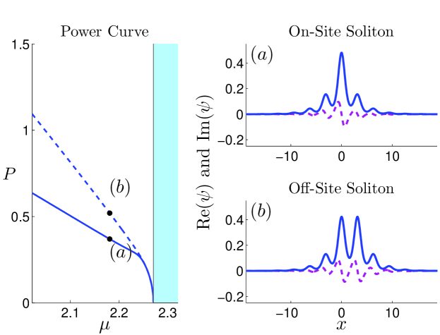
Figure 1: (Left) Power curve for the two families of solitons which bifurcate from the lowest band edge of the periodic potential (2.4) with $(V_{0},W_{0})$ given in (2.12) and $\sigma=1$. (Right) Example solitons for the on-site (top) and off-site (bottom) branches at the marked points of the power curve. Solid lines: Re($\psi$); dashed lines: Im($\psi$).

The above perturbation solution can be continued to all powers in $\epsilon$, which would seem to suggest that for every $x_{0}=X_{0}/\epsilon$ there exists a family of solitons parameterized by $\mu$ that bifurcates from the band edge. This, however, is not the case; a discrepancy studied in [22, 24, 28] for the case of conservative periodic potentials. Instead, only two possible solution families exist. For $\mathcal{PT}$-symmetric periodic potentials they correspond to $x_{0}=0,~{}\pi/2$, as shown in Fig. 1. Here the example periodic potential is (2.4) with

$$V_{0}=6,\quad W_{0}=0.25,$$ (2.12)

the nonlinearity is chosen to be self-focusing ($\sigma=1$), and soliton families are represented by their power curves, where the power is defined as $P(\mu)=\int_{-\infty}^{\infty}|\psi(x;\mu)|^{2}{\rm d}x$. The lower power curve corresponds to solitons centered at $x_{0}=0$ (referred to as on-site solitons), and the upper curve corresponds to solitons centered at $x_{0}=\pi/2$ (referred to as off-site solitons). On-site solitons are $\mathcal{PT}$-symmetric with respect to the origin, while off-site solitons are $\mathcal{PT}$-symmetric with respect to a space shift of half-period $x=\pi/2$. Note that any $\mathcal{PT}$-symmetric periodic potential is also $\mathcal{PT}$-symmetric after a half-period space shift. Hence both on-site and off-site solitons can be said to be $\mathcal{PT}$-symmetric in the underlying $\mathcal{PT}$-symmetric periodic potential.

The explanation for this apparent contradiction rests in terms that are exponentially small in $\epsilon$, which cannot be captured by the above power-series expansion. An exponential-asymptotics approach was developed for conservatives periodic potentials in [22, 24, 25], based on the method used to study soliton solutions of the fifth-order Korteweg-de Vries equation [26]. In this article we develop this exponential asymptotics analysis for complex $\mathcal{PT}$-symmetric periodic potentials.

3 The Fourier transform

The wavepacket solutions of Eq. (2.3) in the bandgap are such that if they decay exponentially in one direction, say upstream or as $x\rightarrow-\infty$, then they would generically grow expontentially in the other direction, say downstream or $x\rightarrow+\infty$. These growing tails are exponentially small in $\epsilon$. Once we have worked out these exponentially small tail terms, the center position $x_{0}$ of the envelope can be determined by requiring that these terms vanish. To do so, we move to the Fourier domain, where the exponentially small tail contributions map to poles with exponentially small strength.

We consider the Fourier transform of the solution $\psi(x,X)$ with respect to the slow space variable $X$, written formally as

$$\widehat{\psi}(x,K)=\frac{1}{2\pi}\displaystyle\int_{-\infty}^{\infty}\psi(x,X){\rm e}^{-{i}KX}{\rm d}X.$$

Since $\psi(x,X)$ is complex, we also introduce the Fourier transform of $\psi^{*}(x,X)$,

$$\widehat{\psi^{*}}(x,K)=\frac{1}{2\pi}\displaystyle\int_{-\infty}^{\infty}\psi^{*}(x,X){\rm e}^{-{i}KX}{\rm d}X.$$

Substituting the perturbation series (2.8) into these transforms, we get

$$\widehat{\psi}=\epsilon\frac{\alpha\beta}{2}{\rm e}^{-{i}KX_{0}}{\rm sech}\left(\frac{\pi}{2}\beta K\right)\left[p(x)+{i}\epsilon K\nu(x)+\ldots\right],$$ (3.1)

and

$$\widehat{\psi^{*}}=\epsilon\frac{\alpha\beta}{2}{\rm e}^{-{i}KX_{0}}{\rm sech}\left(\frac{\pi}{2}\beta K\right)\left[p^{*}(x)+{i}\epsilon K\nu^{*}(x)+\ldots\right],$$ (3.2)

which are disordered when $\kappa\equiv\epsilon K=O(1)$. Thus we replace them by uniformly valid expressions

$$\widehat{\psi}(x,\kappa)=\epsilon{\rm e}^{-{i}\kappa x_{0}}{\rm sech}\left(\frac{\pi\beta\kappa}{2\epsilon}\right)U_{1}(x,\kappa;\epsilon),$$ (3.3)

and

$$\widehat{\psi^{*}}(x,\kappa)=\epsilon{\rm e}^{-{i}\kappa x_{0}}{\rm sech}\left(\frac{\pi\beta\kappa}{2\epsilon}\right)U_{2}(x,\kappa;\epsilon),$$ (3.4)

where

$$U_{1}(x,\kappa;\epsilon) =p(x)+{i}\kappa\nu(x)+\ldots,\qquad|\kappa|\ll 1,$$

$$U_{2}(x,\kappa;\epsilon) =p^{*}(x)+{i}\kappa\nu^{*}(x)+\ldots,\quad|\kappa|\ll 1.$$

We now derive the governing equations for $(U_{1},U_{2})$ by taking the Fourier transform of equation (2.7), which yields

$$L_{0}\widehat{\psi}+2{i}\kappa\widehat{\psi}_{x}-\kappa^{2}\widehat{\psi}+\sigma\widehat{\psi^{2}\psi^{*}}+\epsilon^{2}\eta\widehat{\psi}=0.$$

A similar equation can be obtained for $\widehat{\psi^{*}}$. Substituting in the expressions (3.3)-(3.4) we find that $(U_{1},U_{2})$ satisfy

$$0= L_{0}U_{1}+2{i}\kappa U_{1x}+(\epsilon^{2}\eta-\kappa^{2})U_{1}+\sigma\>{\rm cosh}\frac{\pi\beta\kappa}{2\epsilon}\times$$

$$\int_{-\infty}^{\infty}\int_{-\infty}^{\infty}{\rm sech}\frac{\pi\beta(\kappa-r)}{2\epsilon}{\rm sech}\frac{\pi\beta(r-s)}{2\epsilon}{\rm sech}\frac{\pi\beta s}{2\epsilon}\;U_{1}(\kappa-r)U_{1}(r-s)U_{2}(s)\>{\rm d}r{\rm d}s,$$ (3.5)

$$0= L_{0}^{*}U_{2}+2{i}\kappa U_{2x}+(\epsilon^{2}\eta-\kappa^{2})U_{2}+\sigma\>{\rm cosh}\frac{\pi\beta\kappa}{2\epsilon}\times$$

$$\int_{-\infty}^{\infty}\int_{-\infty}^{\infty}{\rm sech}\frac{\pi\beta(\kappa-r)}{2\epsilon}{\rm sech}\frac{\pi\beta(r-s)}{2\epsilon}{\rm sech}\frac{\pi\beta s}{2\epsilon}\;U_{2}(\kappa-r)U_{2}(r-s)U_{1}(s)\>{\rm d}r{\rm d}s.$$ (3.6)

4 Poles of the Fourier solution

We are concerned with the behavior near the singularities of $U_{1}(x,\kappa;\epsilon)$ which account for the growing tails of exponentially small amplitude in the physical space. Singularities of $U_{1}$ are expected to occur near values of $\kappa=\kappa_{0}$ where the linear part of equation (3.5) is zero,

$$L_{0}\phi+2{i}\kappa_{0}\phi_{x}-\kappa_{0}^{2}\phi=0.$$

A change of variables $\phi={\rm e}^{-{i}\kappa_{0}x}\widetilde{\phi}$ leaves us with

$$L_{0}\widetilde{\phi}=0,$$

which has a single bounded solution $\widetilde{\phi}=p(x)$, the Bloch mode at band edge. Since $\phi$ should have period matching $p(x)$, $\kappa_{0}$ must be an even integer. This results in poles when $\kappa_{0}=\pm 2,\pm 4,\pm 6,\cdots$. The dominant contributions to the solution come from the nearest poles to zero at $\kappa_{0}=\pm 2$.

Looking for the behavior of the solution $U_{1}(x,\kappa;\epsilon)$ near $\kappa_{0}=2$, we introduce a local variable

$$\xi=\frac{\kappa-\kappa_{0}}{\epsilon},$$ (4.1)

that is $\kappa=\kappa_{0}+\epsilon\xi$. In this region we expand the solution to integral equations (3.5)-(3.6) as (see [22])

$$U_{1}=\frac{{\rm e}^{-{i}\kappa_{0}x}}{\epsilon^{4}}\left[\Phi_{1}(\xi)p(x)+\epsilon{i}\xi\Phi_{1}(\xi)\nu(x)+O(\epsilon^{2})\right],$$ (4.2)

$$U_{2}=\frac{{\rm e}^{-{i}\kappa_{0}x}}{\epsilon^{4}}\left[\Phi_{2}(\xi)p^{*}(x)+\epsilon{i}\xi\Phi_{2}(\xi)\nu^{*}(x)+O(\epsilon^{2})\right].$$ (4.3)

The dominant contribution to the double integrals in equations (3.5)-(3.6) comes from three regions: (i) $r\sim 0$, $s\sim 0$, (ii) $r\sim\kappa$, $s\sim 0$, and (iii) $r\sim\kappa$, $s\sim\kappa$. Calculation of these contributions follows that in [22]. Under the notations

$$U_{1}={\rm e}^{-{i}\kappa_{0}x}{\cal U}_{1},\quad U_{2}={\rm e}^{-{i}\kappa_{0}x}{\cal U}_{2},$$

the simplified integral equations in this region become

$$0 =L_{0}{\cal U}_{1}+\epsilon 2{i}\xi{\cal U}_{1x}+\epsilon^{2}\left(\eta-\xi^{2}\right){\cal U}_{1}$$

$$+\frac{\sigma(\alpha\beta)^{2}}{2\epsilon^{2}}|p(x)|^{2}p(x)\int_{-\infty}^{\infty}{\rm e}^{\pi\beta r/2}r{\rm csch}\left(\frac{\pi\beta r}{2}\right)\left[2\Phi_{1}(\xi-r)+\Phi_{2}(\xi-r)\right]{\rm d}r,$$

$$0 =L_{0}^{*}{\cal U}_{2}+\epsilon 2{i}\xi{\cal U}_{2x}+\epsilon^{2}\left(\eta-\xi^{2}\right){\cal U}_{2}$$

$$+\frac{\sigma(\alpha\beta)^{2}}{2\epsilon^{2}}|p(x)|^{2}p^{*}(x)\int_{-\infty}^{\infty}{\rm e}^{\pi\beta r/2}r{\rm csch}\left(\frac{\pi\beta r}{2}\right)\left[2\Phi_{2}(\xi-r)+\Phi_{1}(\xi-r)\right]{\rm d}r.$$

Substituting the expansions (4.2)-(4.3) into these equations, the terms at orders $\epsilon^{-4}$ and $\epsilon^{-3}$ automatically balance. At order $\epsilon^{-2}$, the solvability conditions yield the following integral equations for $\Phi_{1}$ and $\Phi_{2}$,

$$(1+\beta^{2}\xi^{2})\Phi_{1}-\beta^{2}\int_{-\infty}^{\infty}{\rm e}^{\pi\beta r/2}r{\rm csch}\frac{\pi\beta r}{2}\left[2\Phi_{1}(\xi-r)+\Phi_{2}(\xi-r)\right]{\rm d}r=0,$$ (4.4)

$$(1+\beta^{2}\xi^{2})\Phi_{2}-\beta^{2}\int_{-\infty}^{\infty}{\rm e}^{\pi\beta r/2}r{\rm csch}\frac{\pi\beta r}{2}\left[2\Phi_{2}(\xi-r)+\Phi_{1}(\xi-r)\right]{\rm d}r=0.$$ (4.5)

This is a system of two linear homogeneous Fredholm integral equations. To solve it, we introduce the integral transform

$$\Phi_{n}(\xi)=\int_{0}^{\pm{i}\infty}e^{-s\beta\xi}\phi_{n}(s)\,{\rm d}s,\quad n=1,2,$$ (4.6)

where the plus sign is for $\mbox{Im}(\xi)<0$ and the minus sign for $\mbox{Im}(\xi)>0$. Inserting this integral transform into (4.4)-(4.5) and performing integration by parts, we find that $(\phi_{1},\phi_{2})$ satisfy the following differential equations [22]

$$\frac{{\rm d}^{2}\phi_{1}}{{\rm d}s^{2}}+\phi_{1}-\frac{4}{\sin^{2}s}\phi_{1}-\frac{2}{\sin^{2}s}\phi_{2}=0,$$ (4.7)

$$\frac{{\rm d}^{2}\phi_{2}}{{\rm d}s^{2}}+\phi_{2}-\frac{4}{\sin^{2}s}\phi_{2}-\frac{2}{\sin^{2}s}\phi_{1}=0.$$ (4.8)

Performing dominant balance of these equations around $s\sim 0$ and requiring the integrals in (4.6) to converge, we find that $\phi_{1}$ and $\phi_{2}$ have the same small-$s$ behavior,

$$\phi_{n}\to\chi s^{3},\quad s\to 0\quad(n=1,2),$$

where $\chi$ is a certain constant. Together with the fact that equations (4.7)-(4.8) are symmetric in $\phi_{1}$ and $\phi_{2}$, we see that solutions $\phi_{1}$ and $\phi_{2}$ must be identical, thus

$$\Phi_{1}(\xi)=\Phi_{2}(\xi)\equiv\Phi(\xi).$$

Under this reduction, integral equations (4.4)-(4.5) reduce to

$$(1+\beta^{2}\xi^{2})\Phi-3\beta^{2}\int_{-\infty}^{\infty}{\rm e}^{\pi\beta r/2}r{\rm csch}\frac{\pi\beta r}{2}\Phi(\xi-r){\rm d}r=0,$$ (4.9)

which has been solved before [22, 26]. Its exact solution in the region $\left|{\rm Im}(\xi)\right|\geq 1/\beta$ is given by

$$\Phi(\xi)=\frac{6\beta^{4}}{1+\beta^{2}\xi^{2}}\int_{0}^{\pm{i}\infty}\frac{1}{\sin^{2}s}\phi(s){\rm e}^{-s\beta\xi}{\rm d}s,$$ (4.10)

$$\phi(s)=C\left(\frac{2}{\sin s}+\frac{\cos^{2}s}{\sin s}-\frac{3s\cos s}{\sin^{2}s}\right),$$

where $C$ is a constant. Clearly this solution has simple-pole singularities at $\xi=\pm{i}/\beta$. Since the integral of (4.10) at these points is equal to $-C/6$, we see that

$$\Phi(\xi)\sim-\frac{C\beta^{4}}{1+\beta^{2}\xi^{2}},~{}~{}{\rm for}~{}\xi\to\pm\frac{{i}}{\beta}.$$

Utilizing this equation and recalling the scaling (4.1), we obtain the following singular behaviors for the Fourier solutions $\widehat{\psi}(x,K)$ and $\widehat{\psi^{*}}(x,K)$,

$$\widehat{\psi}(x,K)\sim\frac{\beta^{3}C}{\epsilon^{3}}e^{-\pi\beta\kappa_{0}/2\epsilon}e^{\mp X_{0}/\beta}\frac{e^{-i\kappa_{0}(x+x_{0})}}{K-\frac{\kappa_{0}}{\epsilon}\pm\frac{i}{\beta}}p(x)\qquad(K\to\frac{\kappa_{0}}{\epsilon}\mp\frac{i}{\beta}),$$ (4.11)

$$\widehat{\psi^{*}}(x,K)\sim\frac{\beta^{3}C}{\epsilon^{3}}e^{-\pi\beta\kappa_{0}/2\epsilon}e^{\mp X_{0}/\beta}\frac{e^{-i\kappa_{0}(x+x_{0})}}{K-\frac{\kappa_{0}}{\epsilon}\pm\frac{i}{\beta}}p^{*}(x)\qquad(K\to\frac{\kappa_{0}}{\epsilon}\mp\frac{i}{\beta}).$$ (4.12)

Then from the symmetry relation $[\widehat{\psi}(x,K)]^{*}={\widehat{\psi}}^{*}(x,-K^{*})$ of complex functions $\psi(x,X)$, it follows that

$$\widehat{\psi}(x,K)\sim-\frac{\beta^{3}C^{*}}{\epsilon^{3}}e^{-\pi\beta\kappa_{0}/2\epsilon}e^{\mp X_{0}/\beta}\frac{e^{i\kappa_{0}(x+x_{0})}}{K+\frac{\kappa_{0}}{\epsilon}\pm\frac{i}{\beta}}p(x)\qquad(K\to-\frac{\kappa_{0}}{\epsilon}\mp\frac{i}{\beta}).$$ (4.13)

It remains to determine the constant $C$. To do so, we match the large-$\xi$ asymptotics of $U_{1}$ to the solution $U_{1}$ in the region where $\kappa=O(1)$ but away the singularity at $\kappa\approx\kappa_{0}$. Notice that for $|\xi|\rightarrow\infty$ the main contribution of the integral in solution (4.10) comes from the region $s\sim 0$ where $\phi(s)\sim\frac{2}{5}Cs^{3}$. This yields

$$\Phi(\xi)\rightarrow\frac{12C}{5}\frac{1}{\xi^{4}},~{}~{}{\rm for}~{}|\xi|\rightarrow\infty.$$

Putting this in terms of $U_{1}$ and $U_{2}$, we find the follow asymptotic behaviors for the inner solutions around $\kappa\sim\kappa_{0}$,

$$U_{1}(x,\kappa)\sim\frac{12C}{5}\frac{p(x)}{(\kappa-\kappa_{0})^{4}}{\rm e}^{-{i}\kappa_{0}x},\qquad\kappa\sim\kappa_{0},$$ (4.14)

and

$$U_{2}(x,\kappa)\sim\frac{12C}{5}\frac{p^{*}(x)}{(\kappa-\kappa_{0})^{4}}{\rm e}^{-{i}\kappa_{0}x},\qquad\kappa\sim\kappa_{0}.$$ (4.15)

This behavior we match to the solution of (3.5)-(3.6) in the outer region, $\kappa=O(1)$, in section 5.

5 Fourier solution away from poles

Since the strength of the poles cannot be determined uniquely from the local behavior we look to match the asymptotic behavior of the near pole solutions (4.14) to the solution of equations (3.5)-(3.6) for $\kappa=O(1)$ away from these poles. The main contribution of the double integrals in (3.5)-(3.6) now comes from the triangular region $0<s<\kappa$, $0<s<r$ when $\kappa>0$ and $\kappa<s<0$, $r<s<0$ when $\kappa<0$. Over this region,

$${\rm cosh}\frac{\pi\beta\kappa}{2\epsilon}\>{\rm sech}\frac{\pi\beta(\kappa-r)}{2\epsilon}\>{\rm sech}\frac{\pi\beta(r-s)}{2\epsilon}\>{\rm sech}\frac{\pi\beta s}{2\epsilon}\approx 4,$$

thus Eqs. (3.5)-(3.6), to leading order of $\epsilon$, reduce to

$$0 =L_{0}U_{1}+2{i}\kappa U_{1x}-\kappa^{2}U_{1}+4\sigma\int_{0}^{\kappa}\int_{0}^{r}U_{1}(x,\kappa-r)U_{1}(x,r-s)U_{2}(x,s){\rm d}s{\rm d}r,$$ (5.1)

$$0 =L_{0}^{*}U_{2}+2{i}\kappa U_{2x}-\kappa^{2}U_{2}+4\sigma\int_{0}^{\kappa}\int_{0}^{r}U_{2}(x,\kappa-r)U_{2}(x,r-s)U_{1}(x,s){\rm d}s{\rm d}r.$$ (5.2)

We propose to solve these outer integral equations numerically [25]. Since this is a Volterra integral equation, it can be easily tackled by explicit numerical methods. First we discretize $\kappa$, $\kappa_{n}=n\Delta\kappa$, and write

$$U_{1}(x,\kappa_{n}) =U^{(n)}_{1}(x),$$

$$U_{2}(x,\kappa_{n}) =U^{(n)}_{2}(x).$$

Then we approximate the double convolution using the trapezoidal rule. After the terms in the resulting equations are rearranged, $(U^{(n)}_{1},U^{(n)}_{2})$ are found to satisfy the following linear inhomogeneous equations

$$\left[L_{0}+2{i}\kappa_{n}\partial_{x}-\kappa_{n}^{2}+2\sigma U^{(0)}_{1}U^{(0)}_{2}(\Delta\kappa)^{2}\right]U^{(n)}_{1} =-4\sigma F^{(n)}_{1},$$ (5.3)

$$\left[L^{*}_{0}+2{i}\kappa_{n}\partial_{x}-\kappa_{n}^{2}+2\sigma U^{(0)}_{1}U^{(0)}_{2}(\Delta\kappa)^{2}\right]U^{(n)}_{2} =-4\sigma F^{(n)}_{2},$$ (5.4)

where the inhomogeneous terms $F^{(n)}_{1}$ and $F^{(n)}_{2}$ are given by

$$F^{(n)}_{1} =\Delta\kappa^{2}\left[\frac{1}{2}U^{(0)}_{2}I^{(n)}_{1}+\displaystyle\sum_{m=1}^{n-1}U^{(m)}_{2}I^{(n-m)}_{1}\right],$$

$$F^{(n)}_{2} =\Delta\kappa^{2}\left[\frac{1}{2}U^{(0)}_{1}I^{(n)}_{2}+\displaystyle\sum_{m=1}^{n-1}U^{(m)}_{1}I^{(n-m)}_{2}\right],$$

$$I^{(m)}_{j} =\displaystyle\sum_{l=0}^{m-1}U^{(l)}_{j}U^{(m-l)}_{j},\quad{\rm for}~{}1\leq m<n,\hskip 8.5359ptj=1,2,$$

$$I^{(n)}_{j} =\displaystyle\sum_{l=1}^{n-1}U^{(l)}_{j}U^{(n-l)}_{j},\quad j=1,2.$$

The initial conditions $U^{(0,1)}_{1}$ and $U^{(0,1)}_{2}$ can be obtained from equations (3.1)-(3.4) as

$$U^{(0)}_{1}(x) =\frac{\alpha\beta}{2}p(x),$$

$$U^{(1)}_{1}(x) =\frac{\alpha\beta}{2}\left[p(x)+{i}\Delta\kappa~{}\nu(x)\right],$$

$$U^{(0)}_{2}(x) =\frac{\alpha\beta}{2}p^{*}(x),$$

$$U^{(1)}_{2}(x) =\frac{\alpha\beta}{2}\left[p^{*}(x)+{i}\Delta\kappa~{}\nu^{*}(x)\right].$$

Unlike the case of conservative periodic potentials [22], the linear operators on the left sides of equations (5.3)-(5.4) are non-Hermitian, thus conjugate gradient iterations for solving them will not work here. Instead we apply the adjoint linear operators to these equations and turn them into normal equations, which can then be solved by preconditioned conjugate gradient iterations.

Recalling the asymptotic behaviors of inner solutions in equations (4.14)-(4.15), we are motivated to introduce the change of variables

$$\widetilde{U}_{1}(x,\kappa)=(\kappa-\kappa_{0})^{4}U_{1}(x,\kappa),\quad\widetilde{U}_{2}(x,\kappa)=(\kappa-\kappa_{0})^{4}U_{2}(x,\kappa).$$

Then

$$\widetilde{U}_{1}(x,\kappa)\to\frac{12C}{5}p(x){\rm e}^{-{i}\kappa_{0}x},\quad~{}\mbox{as}\ \kappa\to\kappa_{0},$$ (5.5)

$$\widetilde{U}_{2}(x,\kappa)\to\frac{12C}{5}p^{*}(x){\rm e}^{-{i}\kappa_{0}x},\quad\mbox{as}\ \kappa\to\kappa_{0}.$$ (5.6)

At this point we note that $p(x)$ and $\nu(x)$ are both $\mathcal{PT}$-symmetric due to the $\mathcal{PT}$-symmetric periodic potential $V(x)$. Thus the initial conditions for $U_{1}$ and $U_{2}$ are both $\mathcal{PT}$-symmetric. So are the outer equations (5.1)-(5.2) as well. Thus, we see from equations (5.5)-(5.6) that $C$ must be a real constant.

In figure 2 we verify all this numerically. The periodic potential used here is (2.4) with $(V_{0},W_{0})$ values given in (2.12), and $\sigma=1$ (self-focusing nonlinearity). For this potential,

$$\alpha\approx 1.6830,\quad\beta\approx 0.7177.$$

On the left, we plot the numerical solution $\widetilde{U}_{1}(x,\kappa)$ versus $\kappa$ at $x=0$. As predicted in (5.5), this solution indeed approaches a finite theoretical value $\frac{12C}{5}$ when $\kappa\to\kappa_{0}=2$ (recall that $p(x=0)$ has been scaled to one). This numerical curve allows us to determine the $C$ value as

$$C\approx 1.35.$$ (5.7)

In section 7 we are able to independently verify this value of $C$ quantitatively, by comparing our prediction to linear-stability eigenvalues with numerically computed eigenvalues. On the right side of figure 2, we plot the profile of the numerical outer-solution profile $\widetilde{U}_{1}(x,\kappa_{0})$ (dashed red) with the analytical prediction (5.5) (solid blue). The dashed and solid curves are almost indistinguishable, confirming the agreement between numerical solutions and analytical predictions.

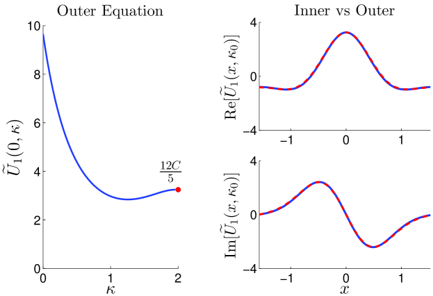
Figure 2: (Left) Numerical solution $\widetilde{U}_{1}(x,\kappa)$ versus $\kappa$ at $x=0$, which converges to the value $\frac{12C}{5}$ when $\kappa\to\kappa_{0}=2$. (Right) Comparison of the numerical outer-solution profile $\widetilde{U}_{1}(x,\kappa_{0})$ (dashed red) with the analytical prediction (5.5) (solid blue). The periodic potential used is (2.4) with $(V_{0},W_{0})$ given in (2.12), and $\sigma=1$.

6 The inverse Fourier transform

The physical solution $\psi(x,X)$ is obtained by taking the inverse Fourier transform of $\widehat{\psi}(x,K)$,

$$\psi(x,X)=\int_{\cal C}\widehat{\psi}(x,K)e^{iKX}{\rm d}K\,.$$

If we require this physical solution to decay upstream ($x\to-\infty$), then the contour $\cal C$ in this inverse Fourier transform should be taken along the line ${\rm Im}(K)=-1/\beta$ and pass below the poles $K=\pm\kappa_{0}/\epsilon-i/\beta$. It should also pass above the pole $K=-i/\beta$ of the ${\rm sech}(\pi\beta K/2)$ term in Eq. (3.3). Then when $x\gg 1$ (downstream), by completing the contour $\cal C$ with a large semicircle in the upper half plane, we pick up dominant contributions from the pole singularities at $K=\pm\kappa_{0}/\epsilon-i/\beta$ and $K=-i/\beta$. Utilizing the pole-singularity solutions (4.11), (4.13), collecting these pole contributions and recalling the reality of $C$, the wave profile of the solution far downstream is then found to be

$$\psi\sim 2\epsilon\alpha\hskip 1.42271pte^{-(X-X_{0})/\beta}p(x)+\frac{4\pi\beta^{3}C}{\epsilon^{3}}e^{-\pi\beta/\epsilon}\sin(2x_{0})e^{(X-X_{0})/\beta}p(x),\quad\,\,x\gg 1/\epsilon.$$ (6.1)

For this solution to be a solitary wave, the growing term in (6.1) must vanish so $\sin\left(2x_{0}\right)=0$. Thus, we find that there are two allowable locations for solitons (relative to the periodic potential),

$$x_{0}=0,\quad\pi/2.$$

That is, the envelope of the solitons must be located either at the point of $\mathcal{PT}$-symmetry ($x_{0}=0$), or half-a-period away from the point of $\mathcal{PT}$-symmetry ($x_{0}=\pi/2$). The resulting two families of solitons are also $\mathcal{PT}$-symmetric with respect to either $x_{0}=0$ or $x_{0}=\pi/2$. These two soliton families are precisely the ones which were found numerically for the sample periodic potential (2.4) in figure 1.

Finally, if one wishes to obtain wave packets $\psi(x,X)$ which decay for $x\to+\infty$ but contain a growing tail for $x\ll-1$, then the contour $\cal C$ in the inverse Fourier transform should be taken along the line ${\rm Im}(K)=1/\beta$ and pass above the poles $K=\pm\kappa_{0}/\epsilon+i/\beta$ and below the pole $K=i/\beta$. Then when $x\ll-1$, by completing the contour $\cal C$ with a large semicircle in the lower half plane and picking up dominant pole contributions from equations (4.11) and (4.13), the wave profile of the solution for $x\ll-1$ is found to be

$$\psi\sim 2\epsilon\hskip 1.13791pt\alpha\hskip 1.42271pte^{(X-X_{0})/\beta}p(x)-\frac{4\pi\beta^{3}C}{\epsilon^{3}}e^{-\pi\beta/\epsilon}\sin(2x_{0})e^{-(X-X_{0})/\beta}p(x),\quad\,\,x\ll-1/\epsilon.$$ (6.2)

7 Connection to stability

We now turn our attention to the linear-stability problem of these two soliton families near band edges. When these solitons bifurcate out from a band edge, a pair of exponentially small eigenvalues bifurcate out from the origin [22]. Using the tail formula (6.1) we are able derive an analytic approximation for these eigenvalues, and thus, by comparison with the numerically computed eigenvalues, verify the validity of our formula for the exponentially small tail as well as the numerical computation of the outer equation.

Let $\psi_{s}(x)=\psi(x;x_{0s})$ be a soliton solution of equation (2.3) with center at $x_{0}=x_{0s}$, which decays to zero as $x\rightarrow\pm\infty$. To study its linear stability we perturb this soliton as

$$\Psi={\rm e}^{-{i}\mu t}\left[\psi_{s}+w_{1}(x)\hskip 1.42271pt{\rm e}^{\lambda t}+w_{2}^{*}(x)\hskip 1.42271pt{\rm e}^{\lambda^{*}t}\right],$$

where $|w_{1}|,|w_{2}|\ll|\psi_{s}|$. After substitution into equation (2.3) and linearizing, we arrive at the eigenvalue problem

$${i}{\cal L}W=\lambda W,$$ (7.1)

where $W=[w_{1}~{}w_{2}]^{T}$ (the superscript ‘$T$’ representing transpose of a vector),

$${\cal L} =\left(\begin{array}[]{c c}L_{11}&L_{12}\\ L_{21}&L_{22}\end{array}\right),$$

$$L_{11} =\partial_{xx}+\mu-V(x)+2\sigma|u|^{2},$$

$$L_{12} =\sigma u^{2},$$

$$L_{21} =-\sigma\left(u^{2}\right)^{*},$$

$$L_{22} =-\left(\partial_{xx}+\mu-V^{*}(x)+2\sigma|u|^{2}\right).$$

Unlike the eigenvalue problem for conservative potentials [22], here the eigenvalue problem cannot be reduced to one with zero diagonal elements. Thus our treatment will require that we solve a coupled equation at each step.

As we’ve seen, the soliton near the band edge is a low-amplitude wave packet whose envelope is governed by (2.9). While the envelope is translationally invariant, this symmetry is not shared by the full equation (2.1). As such, the zero eigenvalue associated with this translation invariance bifurcates due to the broken symmetry. The eigenvalue we are looking for is exponentially small as $\epsilon\rightarrow 0$, and we construct $W$ as a series expansion in $\lambda$,

$$W=W_{0}+\lambda W_{1}+\lambda^{2}W_{2}+\cdots.$$

In this case, the equations at the first few orders of $\lambda$ are

$${i}{\cal L}W_{0}=0,~{}~{}~{}~{}{i}{\cal L}W_{1}=W_{0},~{}~{}~{}~{}{i}{\cal L}W_{2}=W_{1}.$$

At $O(1)$ the solution for $W_{0}$ is

$$W_{0}=\left[\left.\frac{\partial\psi}{\partial x_{0}}\right|_{x_{0}=x_{0s}}~{}~{}~{}\left.\left(\frac{\partial\psi}{\partial x_{0}}\right)^{*}\right|_{x_{0}=x_{0s}}\right]^{T},$$

which can be verified by taking the derivative of (2.3) with respect to the center parameter $x_{0}$. To first order in $\epsilon$ the $W_{0}$ solution may be approximated as

$$\left.\frac{\partial\psi}{\partial x_{0}}\right|_{x_{0}=x_{0s}}\sim-\epsilon^{2}A^{\prime}(X)p(x).$$

If we use the asymptotic formula for the downstream tail (6.1) we find that for $x\gg 1/\epsilon$, $W_{0}$ contains a growing tail

$$\left.\frac{\partial\psi}{\partial x_{0}}\right|_{x_{0}=x_{0s}}\sim\cos(2x_{0s})\frac{8\pi\beta^{3}C}{\epsilon^{3}}{\rm e}^{-\pi\beta/\epsilon}{\rm e}^{(X-X_{0s})/\beta}p(x),\quad x\gg 1/\epsilon.$$

At $O(\lambda)$ we set

$$W_{1}=[{i}w^{(1)}~{}~{}~{}-{i}w^{(1)*}]^{T},$$

and further expand $w^{(1)}$ as a perturbation series in $\epsilon$,

$$w^{(1)}=B(X)p(x)+\epsilon B^{\prime}(X)\nu(x)+\epsilon^{2}\widetilde{w}^{(1)}+\cdots.$$

Inserting this expansion into ${i}{\cal L}W_{1}=W_{0}$ we find that at order $1$ and $\epsilon$ the equation is automatically satisfied, and at order $\epsilon^{2}$ we have

$$L_{0}\widetilde{w}^{(1)}=-[p(x)+2\nu^{\prime}(x)]B^{\prime\prime}(X)-\eta B(X)-\sigma A^{2}(X)B(X)p^{3}(x)+A^{\prime}(X)p(x).$$

The solvability condition for this equation along with the definition for $a$ and $D$ given in (2.10) now results in the following inhomogeneous differential equation for $B$,

$$DB^{\prime\prime}+\eta B+\sigma aA^{2}B=A^{\prime},$$

whose solution is

$$B(X)=\frac{1}{2D}(X-X_{0s})A(X).$$

Proceeding to order $\lambda^{2}$ we let

$$W_{2}=[w^{(2)}~{}~{}~{}w^{(2)*}]^{T},$$

and again expand the solution as a series in $\epsilon$,

$$w^{(2)}=\frac{1}{\epsilon^{2}}\left[F(X)p(x)+\epsilon F^{\prime}(X)\nu(x)+\epsilon^{2}\widetilde{w}^{(2)}+\dots\right].$$

Inserting this expansion into ${i}{\cal L}W_{2}=W_{1}$, at order $\epsilon^{2}$ we arrive at the equation

$$L_{0}\widetilde{w}^{(2)}= -[p(x)+2\nu^{\prime}(x)]F^{\prime\prime}(X)-\eta p(x)F(X)$$

$$-3\sigma A^{2}(X)F(X)p^{3}(x)+\frac{1}{2D}(X-X_{0s})A(X)p(x)$$

for $\widetilde{w}^{(2)}$, which has solvability condition

$$DF^{\prime\prime}+\eta F+3\sigma aA^{2}F=\frac{1}{2D}(X-X_{0s})A.$$ (7.2)

If we require that $F$ decay upstream, then this will result in a solution that grows exponentially downstream

$$F(X)\sim R\>{\rm e}^{(X-X_{0s})/\beta},~{}~{}~{}X\gg 1$$

for some constant $R$. By multiplying both sides of (7.2) by the homogenous solution $A^{\prime}(X)$ and then integrating from $-\infty$ to $X$ we get

$$\int_{-\infty}^{X}A^{\prime}\left[DF^{\prime\prime}+\eta F+3\sigma aA^{2}F\right]{\rm d}\widetilde{X}=\frac{1}{2D}\int_{-\infty}^{X}(X-X_{0s})AA^{\prime}{\rm d}\widetilde{X}.$$ (7.3)

After substituting in the expression for $A$ given in (2.11) as well as the asymptotic behavior of $F$, we perform integration by part on both sides of equation (7.3) to find $R=\alpha/8\beta$. This, in turn, gives us

$$w^{(2)}\sim\frac{1}{\epsilon^{2}}\frac{\alpha}{8\beta}{\rm e}^{(X-X_{0s})/\beta}p(x),\quad X\gg 1.$$

We can now balance the growing tail in $W_{0}$ with the growing tail in $W_{2}$ so that $W$ is bounded. This balancing yields

$$\lambda^{2}=-\cos(2x_{0s})C\frac{64\pi\beta^{4}}{\alpha\epsilon}{\rm e}^{-\pi\beta/\epsilon}.$$ (7.4)

Thus, this eigenvalue is imaginary (stable) for the soliton family with $\cos(2x_{0s})C>0$ and real (unstable) for the other soliton family, and its magnitude is exponentially small. In this paper, the soliton family with $\cos(2x_{0s})C>0$ is called the on-site family, and the one with $\cos(2x_{0s})C<0$ is called the off-site family.

A comparison of the analytical prediction (7.4) to numerical eigenvalues for the family of on-site solitons (with $x_{0s}=0$) from figure 1 is shown in figure 3 for the example potential (2.4). We can see from the left panel that the numerical eigenvalues are well approximated by the analytic prediction. Notice that the analytical eigenvalue formula contains the constant $C$, and the ratio of $-\lambda^{2}/[64\pi\beta^{4}{\rm e}^{-\pi\beta/\epsilon}/\alpha\epsilon]$ approaches $C$ as $\epsilon\to 0$. In the right panel of figure 3 we find that this ratio indeed approaches the value of $C$ found in the earlier (5.7). This gives us a quantitative verification for the asymptotic formula (6.1) for the downstream behavior of $\psi(x)$.

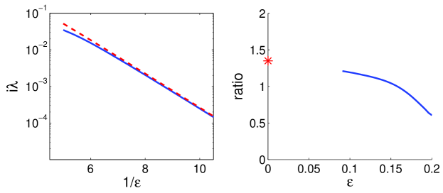
Figure 3: (Left) Comparison of numerical (solid blue) and analytical (dashed red) eigenvalues for on-site solitons of figure 1. (Right) Ratio of $-\lambda^{2}/[64\pi\beta^{4}{\rm e}^{-\pi\beta/\epsilon}/\alpha\epsilon]$ versus $\epsilon$ using numerical $\lambda$ values. The red asterisk marks the $C$ value (5.7) from outer-equation computation.

The above eigenvalue calculations show that the off-site solitons near band edges are always linearly unstable due to the unstable eigenvalue from (7.4). For on-site solitons near band edges, the eigenvalues from (7.4) are stable. However, other unstable eigenvalues may appear which can still render the soliton unstable. For instance, if part of the Bloch bands of the periodic potential is complex, then the linear-stability operator ${i}{\cal L}$ will possess unstable continuous eigenvalues. For another instance, if some segment of ${i}{\cal L}$’s continuous eigenvalues is embedded inside another segment of ${i}{\cal L}$’s continuous eigenvalues on the imaginary axis when $\epsilon=0$, then when $\epsilon\neq 0$, complex discrete eigenvalues might also bifurcate out from the imaginary axis. For on-site solitons originating from the lowest Bloch-band edge into the semi-infinite gap, continuum-embedding does not occur. In this case, when the Bloch bands of the periodic potential are all-real, then the family of on-site solitons near this band edge are indeed linearly stable. However, for on-site solitons originating from other band edges, their stability still needs careful examination.

8 Construction of multi-soliton bound states

By eliminating the growing tail terms we are able to locate the center of the soliton envelope, however more information than just this can be gleaned from the exponentially small tail terms. By matching the downstream growing tail of a wavepacket with the upstream decaying tail of another neighboring wavepacket we can analytically construct multi-soliton bound states. This technique has been used successfully for the construction of multi-soliton bound states for one- and two-dimensional conservative systems [23, 24, 25, 26], and the same basic analysis holds for the $\mathcal{PT}$ symmetric case.

Consider two wavepackets centered at $x_{1}=X_{1}/\epsilon$ (left) and $x_{2}=X_{2}/\epsilon$ (right) respectively. The left wavepacket decays for $x-x_{1}\ll-1$ and has a growing exponential tail for $x-x_{1}\gg 1$, and the right wavepacket decays for $x-x_{2}\gg 1$ and has a growing exponential tail for $x-x_{2}\ll-1$. In the intermediate range, $x_{1}\ll x\ll x_{2}$, the decaying and growing tails of the two wavepackets must match in order for them to form a bound state. In this matching region, the left wavepacket’s asymptotics is given by (6.1) with $x_{0}$ replaced by $x_{1}$, and the right wavepacket’s asymptotics is given by (6.2) with $x_{0}$ replaced by $x_{2}$. Matching of these asymptotics results in the following system of equations

$$2\epsilon\alpha{\rm e}^{-(X-X_{1})/\beta}p(x) =\mp\frac{4\pi\beta^{3}C}{\epsilon^{3}}{\rm e}^{-\pi\beta/\epsilon}\sin\left(2x_{2}\right){\rm e}^{-(X-X_{2})/\beta}p(x),$$

$$2\epsilon\alpha{\rm e}^{(X-X_{2})/\beta}p(x) =\pm\frac{4\pi\beta^{3}C}{\epsilon^{3}}{\rm e}^{-\pi\beta/\epsilon}\sin\left(2x_{1}\right){\rm e}^{(X-X_{1})/\beta}p(x),$$

where ‘$\mp$’ comes from a possible $\pi$ phase shift between the neighboring wavepackets. After some reductions, this set of equations become

$$\sin\left(2x_{1}\right)=-\sin\left(2x_{2}\right)=\pm\frac{\alpha\epsilon^{4}}{2\pi\beta^{3}C}{\rm e}^{\pi\beta/\epsilon}{\rm e}^{\epsilon(x_{1}-x_{2})/\beta},$$ (8.1)

which are identical to the matching conditions found previously [23]. As was explained there, this system of equations admits an infinite number of solutions for each fixed $\epsilon>0$. By varying $\epsilon$, infinite families of two-soliton bound states are obtained. Furthermore, for equation (8.1) to admit solutions the absolute value of the right-hand side must be less than or equal to 1. Since this is not the case in the limit $\epsilon\rightarrow 0$ for any finite separation, $x_{2}-x_{1}$, we see that every solution family bifurcates at some critical distance away from the band edge, i.e., when $\epsilon$ is above a certain critical value $\epsilon_{c}$.

Equation (8.1) admits two types of solutions. The first type is

$$x_{1}=\frac{\pi}{2}-d,\quad x_{2}=N\pi+\frac{\pi}{2}+d$$ (8.2)

for the plus sign (same envelope polarity) and

$$x_{1}=-d,\quad x_{2}=N\pi+d$$ (8.3)

for the minus sign (opposite envelope polarity), where $N$ is an integer, and $0<d<\pi/2$ is determined from the equation

$$\sin 2d=\frac{\alpha\epsilon^{4}}{2\pi\beta^{3}C}{\rm e}^{\pi\beta/\epsilon}{\rm e}^{-\epsilon(N\pi+2d)/\beta}.$$ (8.4)

For the envelope positions (8.2), the resulting two-soliton bound state $\psi(x)$ is $\mathcal{PT}$-symmetric with respect to the bound-state center $x_{c}=(N+1)\pi/2$; for the envelope positions (8.3), $i\psi(x)$ is $\mathcal{PT}$-symmetric with respect to the bound-state center $x_{c}=N\pi/2$. In both cases, the bound states are $\mathcal{PT}$-symmetric (after a horizonal spatial shift).

Numerically we have confirmed the existence of this type of bound states. To demonstrate, we take the periodic potential (2.4) with $(V_{0},W_{0})$ given in (2.12), and $\sigma=1$. Then for $N=5$ and same envelope polarity, this family of two-soliton bound states in the semi-infinite gap is found and presented in figure 4. The power curve (upper left panel) has two connected branches which do not touch the band edge, in agreement with the analysis. The bound states on the lower power branch (lower left panel) are roughly given by two on-site solitons, while the bound states on the upper power branch (lower right panel) are roughly given by two off-site solitons. Notice that these bound states are $\mathcal{PT}$-symmetric with respect to a spatial shift of $3\pi$. When $N$ is varied, the analytical and numerical critical $\epsilon_{c}$ values (in the upper right panel) are also consistent. In addition, their agreement improves for larger $N$, which is expected.

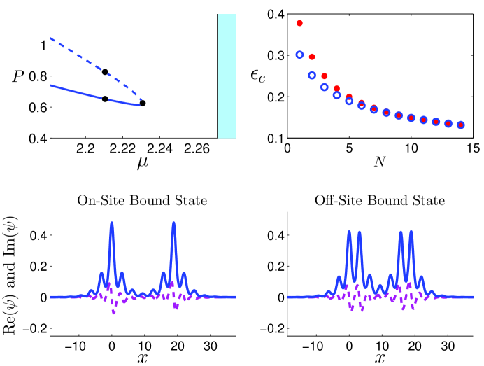
Figure 4: (Upper left) Power curve for the solution family with $N=5$ and same envelope polarity in the semi-infinite gap. (Upper right) Comparison of analytically predicted critical values $\epsilon_{c}$ (blue circles) with numerically obtained values (red dots) at various $N$ values. (Lower panels) Example bound-state solutions at the marked points of the lower and upper power branches. The periodic potential used is (2.4) with $(V_{0},W_{0})$ given in (2.12), and $\sigma=1$.

The second type of solutions admitted by equation (8.1) is

$$x_{1}=-\frac{\pi}{2}-d,\quad x_{2}=N\pi-d$$ (8.5)

for the plus sign (same envelope polarity) and

$$x_{1}=-d,\quad x_{2}=\left(N+\frac{1}{2}\right)\pi-d$$ (8.6)

for the minus sign (opposite envelope polarity), where $N$ is an integer and $0<d<\pi/2$ is determined from the equation

$$\sin 2d=\frac{\alpha\epsilon^{4}}{2\pi\beta^{3}C}{\rm e}^{\pi\beta/\epsilon}{\rm e}^{-\epsilon(N+\frac{1}{2})\pi/\beta}.$$ (8.7)

For these envelope positions, the resulting two-soliton bound states comprise roughly an on-site and off-site solitons, and are thus always non-$\mathcal{PT}$-symmetric under any spatial shift. These non-$\mathcal{PT}$-symmetric bound states, if they were to exist, would contradict the analytical result in [21], which showed that $\mathcal{PT}$-symmetric potentials could not support continuous families of non-$\mathcal{PT}$-symmetric solitary waves.

Numerically, we have found that these on-site and off-site bound states are not true solitary-wave solutions of equation (2.3), in agreement with [21] and contradicting the predictions of equation (8.1). Our numerical verification used Newton-conjugate-gradient iterations [1], together with a multi-precision toolbox for Matlab to resolve the numerical solutions to an accuracy of $10^{-18}$. While there are approximate on-site and off-site bound-state solutions, when investigated using multi-precision (24-digit) calculations, we find that although the residue error can be as small on the order of $10^{-13}$ they are not true solutions. This disagreement between the exponential asymptotics and numerics is a curious phenomenon. Based on this extremely small magnitude of the residue error associated with these approximate solutions, we argue that the non-existence of on-site and off-site bound states in the $\mathcal{PT}$-symmetric periodic potential is due to terms which are smaller than the leading-order exponentially small terms determined here.

9 Conclusion

Solitons in one-dimensional $\mathcal{PT}$-symmetric periodic potentials have been studied using exponential asymptotics. Compared to previous exponential asymptotics for conservative periodic potentials [22, 23, 24], the new feature of the present analysis is that the inner and outer integral equations, (4.4)-(4.5) and (5.1)-(5.2), are both coupled systems due to complex-valued solitons. Nonetheless, these coupled equations can be solved, thus the exponential asymptotics analysis can be carried out. Following this analysis, we show that two soliton families bifurcate out from each Bloch-band edge for either self-focusing or self-defocusing nonlinearity. An asymptotic expression for the eigenvalues associated with the linear stability of these soliton families is also derived. This formula shows that one of these two soliton families (the off-site family) near band edges is always unstable, while the other (on-site) family can be stable. In addition, infinite families of two-soliton $\mathcal{PT}$-symmetric bound states, comprising two on-site or two off-site solitons, have been constructed by matching the exponentially small tails from two neighboring solitons. These analytical predictions were compared with numerics, and good overall agreements were observed. One minor difference is that, while the exponential asymptotics analysis predicts the existence of on-site and off-site two-soliton bound states (which are non-$\mathcal{PT}$-symmetric), numerical computations disprove their existence (see also [21]). Based on the numerical observation that the residue error of those approximate on-site and off-site bound states is extremely small, we argue that the non-existence of true on-site and off-site bound states is due to terms which are smaller than the leading-order exponentially small terms determined in this article.

References

• [1] J. Yang, Nonlinear Waves in Integrable and Nonintegrable Systems (SIAM, Philadelphia, 2010).
• [2] Y.S. Kivshar and G.P. Agrawal, Optical Solitons: From Fibers to Photonic Crystals (Academic Press, San Diego, 2003).
• [3] M. Skorobogatiy and J. Yang, Fundamentals of Photonic Crystal Guiding (Cambridge University Press, Cambridge, UK, 2009).
• [4] O.Β Morsch and M.Β Oberthaler, Dynamics of Bose-Einstein condensates in optical lattices, Rev. Mod. Phys. 78, 179–215 (2006).
• [5] P.G. Kevrekidis, D.J. Frantzeskakis and R. Carretero-Gonzalez, editors, Emergent Nonlinear Phenomena in Bose-Einstein Condensates (Springer, Berlin, 2008).
• [6] C.M. Bender and S. Boettcher, Real spectra in non-Hermitian Hamiltonians having $\mathcal{PT}$symmetry, Phys. Rev. Lett. 80, 5243–5246 (1998).
• [7] A. Ruschhaupt, F. Delgado and J.G. Muga, Physical realization of $\mathcal{PT}$-symmetric potential scattering in a planar slab waveguide, J. Phys. A 38, L171–L176 (2005).
• [8] R. El-Ganainy, K.Β G. Makris, D.Β N. Christodoulides and Z.Β H. Musslimani, Theory of coupled optical $\mathcal{PT}$-symmetric structures, Opt. Lett. 32, 2632–2634 (2007).
• [9] Z.H. Musslimani, K.G. Makris, R. El-Ganainy and D.N. Christodoulides, Optical solitons in $\mathcal{PT}$periodic potentials, Phys. Rev. Lett. 100, 030402 (2008).
• [10] H. Wang and J. Wang, Defect solitons in parity-time periodic potentials, Opt. Express 19, 4030–4035 (2011).
• [11] Z. Lu and Z. Zhang, Defect solitons in parity-time symmetric superlattices, Opt. Express 19, 11457–11462 (2011).
• [12] F.Kh. Abdullaev, Y.V. Kartashov, V.V. Konotop and D.A. Zezyulin, Solitons in $\mathcal{PT}$-symmetric nonlinear lattices, Phys. Rev. A 83, 041805 (RC) (2011).
• [13] S. Nixon, L. Ge and J. Yang, Stability analysis for solitons in $\mathcal{PT}$-symmetric optical lattices, Phys. Rev. A 85, 023822 (2012).
• [14] J. Zeng and Y. Lan, Two-dimensional solitons in $\mathcal{PT}$linear lattice potentials, Phys. Rev. E 85, 047601 (2012).
• [15] C. Li, C. Huang, H. Liu and L. Dong, Multipeaked gap solitons in $\mathcal{PT}$-symmetric optical lattices, Opt. Lett. 37, pp. 4543-4545 (2012).
• [16] R. Driben and B.A. Malomed, Stability of solitons in parity-time-symmetric couplers, Opt. Lett. 36, 4323–4325 (2011).
• [17] D.A. Zezyulin and V.V. Konotop, Nonlinear modes in the harmonic $\mathcal{PT}$-symmetric potential, Phys. Rev. A 85, 043840 (2012).
• [18] F.C. Moreira, F.Kh. Abdullaev, V.V. Konotop and A.V. Yulin, Localized modes in $\chi^{(2)}$ media with $\mathcal{PT}$-symmetric localized potential, Phys. Rev. A 86, 053815 (2012).
• [19] P.G. Kevrekidis, D.E. Pelinovsky and D.Y. Tyugin, Nonlinear stationary states in $\mathcal{PT}$-symmetric lattices, SIAM J. Appl. Dyn. Syst. 12, 1210- 1236 (2013).
• [20] Y.V. Kartashov, Vector solitons in parity-time-symmetric lattices, Opt. Lett. 38, 2600 -2603 (2013).
• [21] J. Yang, Can parity-time-symmetric potentials support families of non-parity-time-symmetric solitons? Stud. Appl. Math. 132, 332–353 (2014).
• [22] G.Β Hwang, T.Β R. Akylas, and J.Β Yang, Gap solitons and their linear stability in one-dimensional periodic media, Physica D 240, 1055–1068 (2011).
• [23] T.Β R. Akylas, G.Β Hwang, and J.Β Yang, From non-local gap solitary waves to bound states in periodic media, Proc. R. Soc. A 468, 116–135 (2012).
• [24] G.Β Hwang, T.Β R. Akylas, and J.Β Yang, Solitary waves and their linear stability in nonlinear lattices, Stud. Appl. Math. 128, 275–299 (2012).
• [25] S. Nixon, T.R. Akylas and J. Yang, Exponential asymptotics for line solitons in two-dimensional periodic potentials, Stud. Appl. Math. 131, 149–178 (2013).
• [26] T.Β S. Yang and T.Β R. Akylas, On asymmetric gravity-capillary solitary waves, J. Fluid Mech. 330, 215–232 (1997).
• [27] D.Β C. Calvo, T.Β S. Yang, and T.Β R. Akylas, On the stability of solitary waves with decaying oscillatory tails, Proc. R. Soc. London A 456, 469–487 (2000).
• [28] D.Β E. Pelinovsky, A.Β A. Sukhorukov and Y.Β S. Kivshar, Bifurcations and stability of gap solitons in periodic potentials, Phys. Rev. E 70, 036618 (2004).