Objective Bayesian Model Discrimination
in Follow-up Experimental Designs

Abstract

An initial screening experiment may lead to ambiguous conclusions regarding the factors which are active in explaining the variation of an outcome variable: thus adding follow-up runs becomes necessary. We propose a fully Bayes objective approach to follow-up designs, using prior distributions suitably tailored to model selection. We adopt a model criterion based on a weighted average of Kullback-Leibler divergences between predictive distributions for all possible pairs of models. When applied to real data, our method produces results which compare favorably to previous analyses based on subjective weakly informative priors. Supplementary materials are available online.

KEY WORDS: Bayesian model selection; Kullback-Leibler divergence; Screening experiment.

1 Introduction

In screening designs the objective is to discover which of the many potential factors are really active, i.e. contribute to explain the variability of a response variable.

In this context, it is customary to assume that the response follows a normal linear regression model, where the predictors are the model-specific main effects together with all interactions up to a specified order (usually two). In this way, for each given set of active factors, there is associated one and only one linear model. If one considers $k$ factors, there exist $2^{k}$ distinct models, including the null model (no factor is active), and the full model (all factors are active).

We adopt a Bayesian approach, wherein each uncertain quantity (such as model, parameter or future observation) is assigned a prior (distribution) which, in the light of data, is updated to a posterior. In particular the Bayesian approach produces a full posterior distribution on the space of all models, unlike in frequentist model selection procedures (e.g. AIC, BIC, or penalized regression methods such as the Lasso).

Often screening designs are based on a limited number of runs, and they may not lead to unequivocal conclusions as to which factors are active, because the posterior probability on model space is not sufficiently concentrated on a few models; and similarly for the induced posterior probability that each factor is active. As a consequence, extra runs are needed to resolve this ambiguity. The issue then becomes finding the combination of factor levels which best discriminates among rival models, and hence factors. This brings us to optimal follow-up designs, which is the core of this paper. In this context, the following intuition can be helpful: a new experiment is most useful whenever the predicted response varies widely across models, because this feature will facilitate model comparison. Accordingly, the follow-up runs are chosen so as to maximize a model discrimination (MD) criterion, see Meyer et al. (1996).

To compute the posterior probability on each model, one requires a prior on model space, as well as a parameter prior on the space of parameters (conditionally on each single model). A notorious difficulty associated with Bayesian model determination is its sensitivity to parameter priors; see O’Hagan & Forster (2004, ch. 7). This remark, and the practical difficulty of specifying distinct subjective priors for each of the entertained models, suggest to adopt an objective Bayes approach (Berger & Pericchi, 2001). The latter program however cannot be carried out using standard noninformative priors for estimation purposes (if for no better reason that they are typically improper); on the other hand proper weakly informative priors, as implemented for instance in Meyer et al. (1996), are also questionable for Bayesian model choice (high sensitivity to prior specification of tuning parameters being an issue); for further discussion see Pericchi (2005).

In this paper we address the problem of choosing follow-up experiments for optimal discrimination among factorial models, using a fully objective Bayesian approach. This seems particularly attractive at the screening stage, especially if prior information is weak. Specifically, we seek to maximize an MD criterion which is a weighted combination of Kullback-Leibler (KL) divergences between predictive distributions (for future follow-up observations conditionally on the available data) for all pairs of models, where the weights are the posterior probabilities of the corresponding model pair; see Box & Hill (1967) for a derivation of this criterion using the notion of expected change in entropy between input and output. A related approach was used by Bingham & Chipman (2007) for identifying most promising screening designs. Their MD criterion however uses the Hellinger distance, rather than KL-divergence, between pairs of (prior) predictive distributions. Because of the structure of MD we decouple the problem into two separate sub-problems: i) finding the posterior probability on model space (which provides the weights of the MD); ii) finding the predictive distributions of future observations (required to compute the KL divergences).

The rest of this paper is organized as follows: Section 2 presents the objective model choice priors; Section 3 introduces the model discrimination criterion; Section 4 applies the methodology to a variety of data sets, and provides comparison with previous analyses. Finally Section 5 contains a brief discussion.

2 Objective model choice priors

2.1 Model assumptions

Consider $k$ categorical factors, and $n$ experimental runs for specific combinations of the factor levels. Let $M_{i}$ be a model which specifies a set of $f_{i}$ active factors ($0\leq f_{i}\leq k$) for the response $y$

$$y\,|\,\beta_{0},\beta_{i},\sigma,M_{i}\sim N_{n}(X_{0}\beta_{0}+X_{i}\beta_{i},\sigma^{2}I_{n}),$$ (1)

where $X_{0}$ represents an $n\times t_{0}$ design matrix containing variables which appear in all models. Typically, $X_{0}=1_{n}$, the $n$-dimensional unit vector; occasionally however, we may want to consider more general versions for $X_{0}$. Both $\beta_{0}$ and $\sigma^{2}$ are regarded as parameters which are “common” across models, while $\beta_{i}$ is the model-specific vector of regression parameters. The $t_{i}$ columns of the matrix $X_{i}$ contain suitable terms representing main effects and interactions of selected factors. The model matrix $[X_{0}\vdots X_{i}]$ is assumed to be of full column rank, so that the number of linearly independent terms in the regression structure cannot exceed $n$. In fractional factorial designs this means that only estimable (non aliased) interactions, up to a desired order, are introduced besides the main effects, conditionally to the constraint that $n>t_{0}+t_{i}$.

2.2 Prior distribution on model space

In this subsection we consider in greater detail the prior on model space. A typical assumption is that each factor is active (i.e. its effect will be included in any particular model) with some probability $\pi$ independently of the other factors. If $M_{i}$ contains $f_{i}$ active factors, $f_{i}\in\{0,1,\ldots,k\}$, then

$$\mathrm{Pr}(M_{i}\,|\,\pi)=\pi^{f_{i}}(1-\pi)^{k-f_{i}}.$$ (2)

Of course $\pi$ is unknown, and from a Bayesian perspective it should be regarded as an uncertain quantity with its own distribution. Assuming that $\pi\sim Beta(a,b)$, then integrating (2) with respect to this prior yields

$$\mathrm{Pr}(M_{i})=\int_{0}^{1}\pi^{f_{i}}(1-\pi)^{k-f_{i}}p(\pi)d\pi=B(a+f_{i},b+k-f_{i})/B(a,b),$$ (3)

where $B(\cdot,\cdot)$ is the usual beta function. Priors belonging to family (3) incorporate a multiplicity adjustment component; see Scott & Berger (2010) for an extensive study.

2.3 Parameter priors

Consider the comparison of two nested models (so that the sampling family under one model is a special case of the other) through the Bayes factor. If one starts with an objective prior developed for estimation purposes, such as the Jeffreys or reference prior, a difficulty arises: since these priors are typically improper, the Bayes factor is undefined. Several attempts have been made to circumvent this problem: intrinsic Bayes factor (Berger & Pericchi, 1996), fractional Bayes factor (O’Hagan, 1995), intrinsic priors Casella & Moreno (2006), expected posterior prior (Perez & Berger, 2002); see Pericchi (2005) for a comprehensive review.

Another approach, whose precursor was essentially Jeffreys (1961), is to develop a proper prior for the parameter “specific” to the current model based on some reasonable intuition, and then test its reasonableness in specific settings using simulation studies and possibly theoretical results. Examples, with reference to variable selection in normal linear models, include Zellner & Siow (1980) on $g$-priors, Liang et al. (2008), Clyde et al. (2011), Maruyama & George (2011); see also Bayarri & Garcia-Donato (2007) for generalized linear models.

Very recently, a different approach was proposed by Bayarri et al. (2012), where criteria that should be satisfied by any model choice prior are first laid out in generality, with special consideration for the objective case. Next, one seeks priors which satisfy these requirements, in the specific setting under investigation. We find this research strategy convincing, and adopt it in this paper to propose a solution for the follow-up experiment.

Recall the structure of model $M_{i}$ presented in (1). On the other hand the null model $M_{0}$ prescribes $y\,|\,\beta_{0},\sigma\sim N_{n}(\beta_{0}X_{0},\sigma^{2}I_{n})$. Consider the following hierarchical $g$-prior for model choice

$$p^{R}(\beta_{0},\beta_{i},\sigma\,|\,M_{i})=p(\beta_{0},\sigma)p^{R}(\beta_{i}\,|\,\beta_{0},\sigma\,|\,M_{i})=\sigma^{-1}\times\int_{0}^{\infty}N_{t_{i}}(\beta_{i}\,|\,0,g\Sigma_{i})p^{R}(g\,|\,M_{i})dg,$$ (4)

where $p(\beta_{0},\sigma)$ is the prior on the common parameters shared by all models, $\Sigma_{i}=\sigma^{2}(V_{i}^{\prime}V_{i})^{-1}$, $V_{i}=(I_{n}-X_{0}(X_{0}^{\prime}X_{0})^{-1}X_{0}^{\prime})X_{i}$ and

$$p^{R}(g\,|\,M_{i})=\frac{1}{2}\left[\frac{1+n}{t_{i}+t_{0}}\right]^{1/2}(g+1)^{-3/2}1_{(\frac{1+n}{t_{i}+t_{0}}-1,\infty)}(g),$$

with $1_{A}(t)=1$ if $t\in A$ and 0 otherwise. Prior (4) has been shown to satisfy all desiderata from an objective model choice perspective; see Bayarri et al. (2012, Section 2) (the superscript “R” stands for “robust prior ”). Notice that (4) is improper; however it scales appropriately when compared to the null model $M_{0}$ so that the resulting Bayes factor for the comparison of $M_{i}$ against $M_{0}$ is meaningful. Its expression is

$$BF_{i0}(y)=\left[\frac{n+1}{t_{i}+t_{0}}\right]^{-t_{i}/2}$$ (5)

$$\times\frac{Q_{i0}(y)^{-(n-t_{0})/2}}{t_{i}+1}{{}_{2}F_{1}}\left[\frac{t_{i}+1}{2};\frac{n-t_{0}}{2};\frac{t_{i}+3}{2};\frac{(1-Q_{i0}(y)^{-1})(t_{i}+t_{0})}{n+1}\right],$$

where ${}_{2}F_{1}$ is the standard hypergeometric function (Abramowitz & Stegun, 1964), and $Q_{i0}(y)=SSE_{i}(y)/SSE_{0}(y)$ is the ratio of the sum of squared errors of models $M_{i}$ and $M_{0}$.

3 The model discrimination criterion

Assuming that one of the entertained models is true, the posterior probability of each model $M_{i}$ can be written in the convenient form

$$\mathrm{Pr}(M_{i}\,|\,y)=\frac{BF_{i0}(y)P_{i0}}{1+\sum_{j\neq 0}BF_{j0}(y)P_{j0}},$$ (6)

where $P_{j0}$ is the prior odds of model $M_{j}$ relative to $M_{0}$ implied by (3), and $BF_{j0}(y)$ is defined in (5). In particular we adopt (3) with $(a=1,b=1)$ for which $P_{j0}=f_{j}!(k-f_{j})!/k!$.

Having computed $\mathrm{Pr}(M_{i}\,|\,y)$, $i=1,\ldots,2^{k}$, a useful by-product is the posterior probability $P_{A}(y)$ that factor $A$ say is active; namely $\sum_{\{M_{j}:\,\mbox{factor A is active}\}}\mathrm{Pr}(M_{j}\,|\,y)$.

In order to determine the $n^{*}$ follow-up runs which best discriminate among potential explanatory models, Meyer et al. (1996) suggested to maximize the following model discrimination (MD) criterion

$$MD=\sum_{i\neq j}\mathrm{Pr}(M_{i}|y)\mathrm{Pr}(M_{j}|y)KL(m(\cdot|y,M_{i}),m(\cdot|y,M_{j})),$$ (7)

where $m(\cdot|y,M_{i})$ is the (posterior) predictive density for the vector of follow-up observations, and

$$KL(f,g)=\int f(x)\log\frac{f(x)}{g(x)}dx$$ (8)

is the Kullback-Leibler divergence of the density $f$ from $g$. Notice that MD is a weighted average of the KL-divergences between all pairs of predictive distributions for the follow-up observations.

Adopting a standard reference prior $p^{N}(\beta_{0},\beta_{i},\sigma\,|\,M_{i})\propto 1/\sigma$ for prediction purposes leads to a closed form expression for the MD criterion, which we label OMD (Objective MD). This is given by

$$OMD=$$ (9)

$$\sum_{i\neq j}\mathrm{Pr}(M_{i}|y)P(M_{j}|y)\frac{1}{2}\left\{tr(V_{j}^{*\,-1}V_{i}^{*})+\frac{n-t_{i}-t_{0}}{SSE_{i}}(\hat{y}_{i}^{*}-\hat{y}_{j}^{*})^{\prime}V_{j}^{*\,-1}(\hat{y}_{i}^{*}-\hat{y}_{j}^{*})-n^{*}\right\},$$

where $\mathrm{Pr}(M_{i}|y)$ is defined in (6), $SSE_{i}$ is the usual residual sum of squares under model $M_{i}$, and the remaining quantities are defined in (12) of Appendix A in the Supplementary Materials, which includes further details. To find the best follow-up runs one has to maximize OMD over all possible $n^{*}$ combinations with repetition from the set of runs of the full factorial design.

Meyer et al. (1996) evaluate MD using (2) with $\pi$ equal to a fixed small value (the recommended choice was $\pi=0.25$) to induce factor sparsity in model selection. Additionally, they chose $p(\beta_{0},\sigma)\propto 1/\sigma$ as we did, while adopting a proper weakly informative Gaussian prior on $\beta_{i}\,|\,\beta_{0},\sigma,M_{i}$, wherein each component of $\beta_{i}$ is assigned a normal distribution with zero expectation and standard deviation $\gamma\sigma$, with $\gamma$ a tuning parameter, which need be specified by the user. We label the resulting criterion CMD (Conventional MD).

OMD has the advantage, with respect to CMD, of being fully Bayes, objective, and based on principled model selection priors. In particular, there is no need to tune hyperparameters, which makes it especially attractive from a practitioner’s point of view. In fact, on the one hand it is well known that model selection is typically highly sensitive to the choice of hyperparameters; on the other hand this prior information is usually hard to elicit in screening experiments.

We have developed Fortran and R-code to find the optimal follow-up runs under OMD. This code relies on existing Fortran and R-code to carry out computations under CMD; see Meyer (1996) and Barrios Zamudio (2013).

4 Applications

4.1 Injection molding experiment

We first consider the experiment on the percentage shrinkage in an injection molding process described in Box et al. (1978, p. 398) which contains eight factors labeled A through H. This experiment was also analyzed in Meyer et al. (1996). The plan is a $2^{8-4}$ fractional factorial resolution IV design with generators I=ABDH=ACEH=BCFH=ABCG.

A preliminary analysis based on normal probability plots, and confirmed by a Bayesian analysis (be it conventional or objective), leads to the conclusion that the potential active factors can be reduced to four, namely A, C, E and H. Accordingly, we follow Box et al. (1978) and collapse the $2^{8-4}$ fractional factorial design on the above factors, thus obtaining a replicated $2^{4-1}$ design with defining relation I=ACEH.

The posterior probabilities that each factor is active are reported in Table 1. They are essentially uniform for the case of three-factor interactions (3FI) both under the conventional and the objective approach; this result is only partly modified in the case of 2FI, where factor A appears unlikely to be active under the conventional approach. It appears that additional runs are needed both to resolve the ambiguity regarding factor A, and to further investigate the role of the remaining factors.

Table 1: Injection molding experiment. Posterior probabilities that factors are active for the $2^{4-1}$ design

	2FI			3FI
Factor	Conventional Approach	Objective Approach		Conventional Approach	Objective Approach
$A$	$0.18$	$0.68$		$0.76$	$0.87$
$C$	$1$	$1$		$0.76$	$0.88$
$E$	$1$	$1$		$0.76$	$0.87$
$H$	$0.91$	$0.95$		$0.76$	$0.87$

Table 8 in the Supplementary materials reports the full $2^{4}$ design in the factors A, C, E, H, with the corresponding runs in the $2^{8-4}$ fractional design. Assuming that $n^{*}=4$ follow-up runs have to be chosen, the number of possible follow-up designs (with replication) from the 16 candidate runs of the $2^{4}$ factorial design in the factors A, C, E, H is 3876.

The five best designs identified by the OMD criterion of formula (9), along with those corresponding to the CMD criterion are shown in Table 2, separately for models having 2FI and 3FI. The CMD criterion was applied using the recommended settings $\pi=0.25$ and $\gamma=2$, and without a block-effect to distinguish between screening and follow-up runs. We also report for completeness the value of the criterion achieved by each single run. Please notice that these values are meaningful for comparison purposes within each criterion, but not between criteria.

Table 2: Injection molding experiment. Top five follow-up designs

	2FI					3FI
Model	CMD	runs	OMD	runs		CMD	runs	OMD	runs
$1$	11.23	9 12 13 16	$51.12$	9 13 15 16		$88.37$	9 11 12 15	$103.41$	9 10 11 13
$2$	$11.08$	9 12 15 16	$49.84$	9 12 13 16		$87.37$	9 12 12 15	$100.39$	9 10 11 12
$3$	$10.99$	11 12 15 16	$49.53$	9 9 13 15		$87.35$	9 9 12 15	$99.03$	9 10 10 11
$4$	$10.92$	9 11 12 16	$49.52$	9 9 13 16		$86.53$	9 12 14 15	$98.34$	9 10 11 16
$5$	$10.87$	12 13 15 16	$48.22$	9 11 13 16		$83.87$	9 11 12 12	$98.09$	9 10 11 11

A common feature is that all follow-up runs belong to the set $\{9,10,\ldots,16\}$, i.e. the set of runs which were not carried out in the initial screening experiment; this is reassuring because those runs were not able to discriminate sufficiently among models. Some differences emerge depending on the number of FI allowed in the models as well as the criterion which is adopted (CMD and OMD), although runs 9 and 11 are broadly recurring.

4.2 Reactor experiment

In this subsection we consider the reactor experiment described in Box et al. (1978, p. 376). Table 9 in the Supplementary Materials reports the complete $2^{5}$ factorial design, including the value of the response variable. This feature makes this experiment especially attractive, because we can actually verify the effectiveness of our approach in identifying active factors, as we detail below.

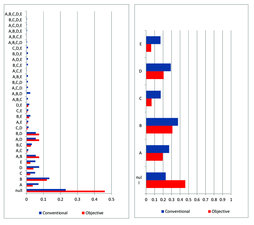
Figure 3: Reactor experiment. Posterior probabilities of models and that factors are active (3FI)

Following Meyer et al. (1996, Section 3), we extract eight runs from the original experiment corresponding to the $2^{5-2}$ Resolution III design with generators I=ABD=ACE, and consider these runs as our initial screening design; see Table 10 in the Supplementary Materials. The five highest posterior probability (top) models based on the objective Bayes approach are reported in Table 3 for models with 2FI. The corresponding results for the case of 3FI are reported in Table 11 in the Supplementary Materials. For the sake of comparison we also included the corresponding results based on the conventional approach derived in Meyer et al. (1996) (setting $\gamma=0.4$ and $\pi=0.25$). The posterior probabilities of all models, and that the factors are active, are also displayed in Figure 1 for the case of 2FI (and Figure 3 in the Supplementary Materials for the case of 3FI).

Table 3: Reactor experiment. Posterior probabilities of top five models and that factors are active (2FI)

	Conventional Approach			Objective Approach
Model	Factors	Posterior probability		Factors	Posterior probability
$1$	$null$	$0.23$		$null$	$0.32$
$2$	$B$	$0.13$		$B,D,E$	$0.10$
$3$	$D$	$0.07$		$B$	$0.08$
$4$	$A$	$0.07$		$A,D$	$0.05$
$5$	$A,D$	$0.05$		$B,D$	$0.05$
	Conventional Approach			Objective Approach
	Factor	Posterior probability		Factor	Posterior probability
	$A$	$0.27$		$A$	$0.28$
	$B$	$0.38$		$B$	$0.47$
	$C$	$0.17$		$C$	$0.15$
	$D$	$0.29$		$D$	$0.39$
	$E$	$0.17$		$E$	$0.21$

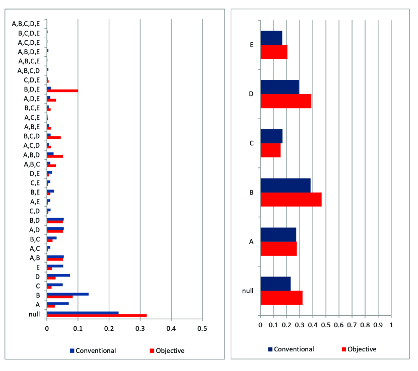
Figure 1: Reactor experiment. Posterior probabilities of models and that factors are active (2FI)

It appears from Figure 1 that the objective Bayes prior tends to favor, relative to the conventional approach, the null model as well as a few models containing three factors. This is due to the different nature of the respective priors on model space. The posterior probabilities that factors are active do not point to a clear-cut conclusion. The highest scoring factor (B) does not even achieve the 50% threshold; the remaining factors trail behind but each one has an appreciable probability of being active. Extra runs are needed in order to solve what appears to be an ambiguous outcome.

To facilitate the comparison with Meyer et al. (1996), we chose to add $n^{*}=4$ follow-up runs. For this problem there exist 52360 four-run designs (with replications) from 32 candidates. The five best follow-up designs selected by the OMD, as well as the CMD, criterion are shown in Table 4 for the case of 2FI.

Table 4: Reactor experiment. Top five follow-up designs (2FI)

Model		CMD	runs		OMD	runs
$1$		$0.5840$	4 10 12 26		$69.85$	11 15 26 29
$2$		$0.5821$	4 12 26 27		$69.73$	15 15 29 30
$3$		$0.5800$	10 12 26 27		$69.71$	11 15 26 30
$4$		$0.5797$	4 11 12 26		$69.63$	11 15 29 30
$5$		$0.5792$	4 10 26 28		$69.42$	11 15 25 30

The best four runs under the OMD criterion only marginally overlap (run 26) with those obtained using CMD; on the other hand they do coincide when models with three-factor interactions are considered; see Table 12 in the Supplementary Materials.

To validate the effectiveness of our approach, we re-run the analysis using all 12 runs (screening and follow-up). To account for potential different experimental conditions, a block effect was added in each linear model. For models having 2FI, the results are summarized in Table 5, and also displayed in Figure 2.

Table 5: Reactor experiment. Posterior probabilities of top five models and that factors are active based on the combined screening and follow-up designs (2FI)

	Conventional Approach			Objective Approach
Model	Factors	Posterior probability		Factors	Posterior probability
$1$	$B,D,E$	$0.73$		$B,D,E$	$0.86$
$2$	$B,D$	$0.09$		$B,D$	$0.05$
$3$	$A,B,D,E$	$0.06$		$B$	$0.04$
$4$	$B,C,D,E$	$0.03$		$null$	$0.01$
$5$	$B$	$0.03$		$B,C,D$	$0.01$
	Conventional Approach			Objective Approach
	Factor	Posterior probability		Factor	Posterior probability
	$A$	$0.08$		$A$	$0.02$
	$B$	$0.97$		$B$	$0.98$
	$C$	$0.06$		$C$	$0.02$
	$D$	$0.94$		$D$	$0.93$
	$E$	$0.83$		$E$	$0.87$

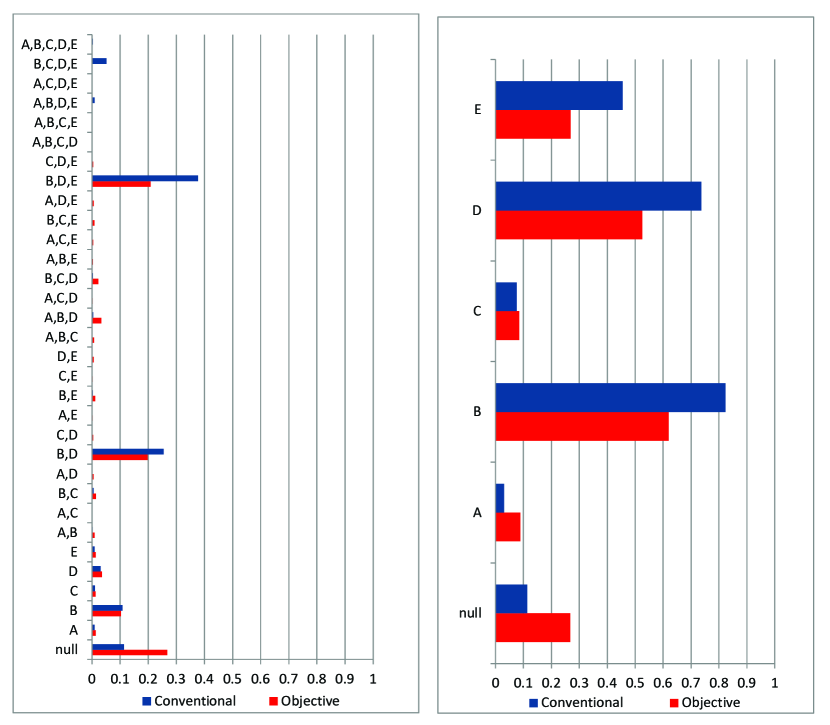
Figure 4: Reactor experiment. Posterior probabilities of models and that factors are active based on the combined screening and follow-up designs (3FI)

It now appears clearly that the only model worth of consideration is the one involving factors B, D and E; these results are also spelled out in the posterior probabilities that factors are active. Table 13 and Figure 4. in the Supplementary Materials illustrate the analysis for models involving three-factor interactions with results broadly similar to those obtained under the 2FI case, the main difference being that factor E appears less likely to be active.

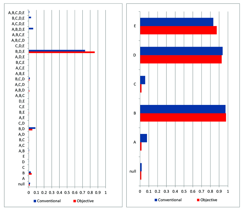
Figure 2: Reactor experiment. Posterior model probabilities of models and that factors are active based on the combined screening and follow-up designs (2FI)

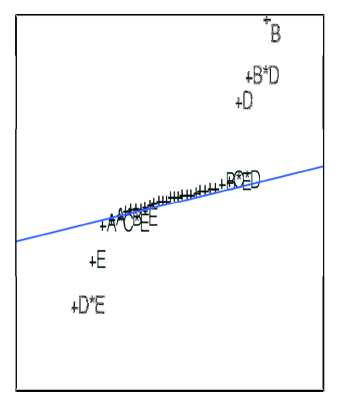
Figure 5: Reactor experiment. Normal probability of contrasts based on the complete set of 32 runs

The above results obtained on the basis of 12 runs are in agreement with those that emerge from the normal probability of the contrasts based on the complete set of 32 runs; see Figure 5 in the Supplementary Materials.

Clearly the follow-up runs greatly contributed to differentiate among factors in terms of their likely activity. Which of the two approaches, conventional or objective, did a better job? Table 6 offers an answer. It computes the normalized Shannon heterogeneity index on the posterior distribution of models after: (1) the screening experiment, and (2) the combined screening and follow-up experiment. Clearly the index is lower in the latter situation, reflecting a reduced heterogeneity (increased concentration). We can see that our objective criterion not only scores lower after (1) and (2) than the conventional one, but it also produces a greater relative reduction (71% against 59%).

Table 6: Reactor experiment. Shannon hetereogenity of model posterior probabilities

		Conventional Approach		Objective Approach
(1): Screening experiment		$0.79$		$0.74$
(2): Screening and follow-up experiment		$0.32$		$0.21$
Relative reduction between (1) and (2)		$59\%$		$71\%$

A similar exercise was performed with respect to the posterior probabilities that the factors are active. In this case, one can no longer use Shannon heterogeneity because the probabilities do not sum to one (the events are not incompatible). Accordingly, we chose the coefficient of variation. In this case situation (2) corresponds to a greater variation. Again OMD provides a higher score than CMD both in case (1) and (2), even though CMD provides a greater improvement in relative terms; see Table 7.

Table 7: Reactor experiment. Coefficient of variation of posterior probabilities that factors are active

		Conventional Approach		Objective Approach
(1): Screening experiment		$0.32$		$0.39$
(2): Screening and follow-up experiment		$0.72$		$0.80$
Relative increase between (1) and (2)		$125\%$		$105\%$

5 Discussion

In this paper we have developed an objective Bayesian method to obtain follow-up designs which are optimal in terms of predictive model discrimination. In order to determine the posterior probability of models, we have employed a multiplicity correction prior on model space, and a principled model selection hierarchical-$g$ prior on the parameters. With regard to prediction, we have relied on a standard reference prior, which produces a closed-form expression for the model discrimination criterion, thus greatly enhancing the computational speed of searching through the space of potential designs. Employing different priors for model selection and prediction implies that our model discrimination criterion will no longer enjoy the theoretical properties described in the original contribution of Box & Hill (1967). However, it will do so at least approximately, because predictions based on the standard reference prior are themselves an approximation to those computed using the model selection prior; see Appendix B of the Supplementary materials. Finally, we remark that the practice of using distinct prior distributions for design and estimation-prediction dates back at least to Tsutakawa (1972). For a more recent example see Han & Chaloner (2004), and references therein, where the motivation is that distinct researchers, with different priors, may be involved in the design and estimation stage.

Our objective Bayes approach requires that the design matrix be of full rank. This is in contrast to what happens in subjective Bayes approaches where this condition can be relaxed at the expense of having to specify a prior covariance matrix on the regression coefficients. Substantive prior information of this kind is usually unavailable, and conventional choices are problematic because model selection is highly sensitive to such prior inputs; see Berger & Pericchi (2001). The requirement that the design matrix be of full rank implies that the set of models that can be entertained -for a given order of interactions- may be smaller than that of all potential models. This difficulty however can be typically overcome by omitting models containing higher-order interactions, or context variables (such as blocking). Since the main goal is obtaining the posterior probability of the active factors -rather than the posterior probability of the models- this simplification seems reasonable.

With regard to the prior on model space presented in Subsection 2.2, we adopted the values $(a=1,b=1)$. Recently the alternative choice $(a=1,b=k+1)$ has been advocated to achieve a stronger sparse modeling effect. This prior, besides performing multiplicity adjustment, is also optimal in terms of concentration of the posterior distribution around the true model; see Castillo & van der Vaart (2012). Having experimented with such prior, the main difference is that the choice $(a=1$, $b=k+1)$ gives more weight to more parsimonious models, relative to $(a=1,b=1)$; however, optimal follow-up runs, are broadly similar in the two cases.

The prior on model space adopted in this paper relies on the assumption of effect forcing whereby if a set of factors is inserted in the model, then all interactions (up to the desired order) must be included. One could relax the assumption of effect forcing, and consider a more flexible approach, as advocated in Bingham & Chipman (2007), through the incorporation of prior opinions on structural aspects of effects such as Effect sparsity, Effect hierarchy and Effect heredity; see also Wolters & Bingham (2011).

The model discrimination criterion used in this work is based on the Kullback-Leibler divergence. Alternative divergence measures could be employed. For instance, within the context of screening experiments, Bingham & Chipman (2007) suggest to use the Hellinger distance, which is symmetric and bounded above. Symmetry is useful from the computational perspective, because it avoids to sum over all pairs of distinct models, while a bounded index makes calibration and interpretation easier. We could implement our method using the Hellinger distance because its expression is also available in closed-form. The choice of the KL-divergence was mostly motivated for comparison purposes with results in the current literature.

Supplementary Materials

Appendix A:

Derivation of KL-divergence between the predictive distributions for the follow-up runs under two models.

Appendix B:

Relationship between the posterior distributions under the hierarchical $g$-prior and the reference prior.

Tables and Figures:

A collection of Tables and Figures complementing those in the main text.

Appendix A: derivation of KL-divergence between the predictive distributions for the follow-up runs under two models

Let $y^{*}$ denote the vector of observations for the $n^{*}$ follow-up runs. Under model $M_{i}$, let $\gamma_{i}^{\prime}=(\beta_{0}^{\prime},\beta_{i}^{\prime})$, and denote with $p^{N}(\gamma_{i},\sigma^{2}\,|\,M_{i})$ an objective estimation prior, where the superscript “N” stands for “noninformative”. Then

$$m(y^{*}\,|\,y,M_{i})=\int\int f(y^{*}\,|\,\gamma_{i},\sigma^{2},M_{i})p^{N}(\gamma_{i},\sigma^{2}\,|\,y,M_{i})d\gamma_{i}d\sigma^{2},$$

where $f(y^{*}\,|\,\gamma_{i},\sigma^{2},M_{i})=N_{n^{*}}(y^{*}\,|\,Z_{i}\gamma_{i},\sigma^{2}I_{n^{*}})$ is the usual Gaussian regression model having set $Z_{i}=[X_{0}\vdots X_{i}]$. Standard computations yield

$$p^{N}(\gamma_{i},\sigma^{2}\,|\,y,M_{i})=p^{N}(\gamma_{i}\,|\,\sigma^{2},y,M_{i})p^{N}(\sigma^{2}\,|\,y,M_{i})$$ (10)

$$= N_{t_{i}+t_{0}}(\gamma_{i}\,|\,\hat{\gamma_{i}},\sigma^{2}(Z_{i}^{\prime}Z_{i})^{-1})IGa(\sigma^{2}\,|\,\frac{n-t_{i}-t_{0}}{2},\frac{SSE_{i}}{2}),$$

where $\hat{\gamma}_{i}$ is the OLS estimate of $\gamma_{i}$ and $IGa(t\,|\,a,b)$ is the inverse gamma density having kernel $(1/t)^{a+1}\exp(-b/t)$.

As a consequence the predictive distribution of $y^{*}$, conditionally on $\sigma^{2}$ and under model $M_{i}$, can be written as

$$m(y^{*}\,|\,\sigma^{2},y,M_{i})=N_{n^{*}}(y^{*}\,|\,\hat{y}_{i}^{*},\sigma^{2}V_{i}^{*}),$$ (11)

where

$$\hat{y}_{i}^{*}=Z_{i}^{*}\hat{\gamma}_{i},\quad V_{i}^{*}=I_{n^{*}}+Z_{i}^{*}(Z_{i}^{\prime}Z_{i})^{-1}Z_{i}^{*\,^{\prime}}.$$ (12)

To compute the KL divergences between pairs of predictive distributions appearing in formula (7) of the paper, we proceed in two steps. First we evaluate the KL divergence conditionally on $\sigma$, and then we take the expectations with respect to the posterior distribution of $\sigma^{2}$.

Conditionally on $\sigma$, the predictive distributions are multivariate normal, and the following Lemma is useful.

Lemma 5.1

Let $m_{0}(\cdot)$ and $m_{1}(\cdot)$ be two $s$-dimensional multivariate Gaussian distributions with expectations $\mu_{0}$ and $\mu_{1}$ and covariance matrices $\Sigma_{0}$ and $\Sigma_{1}$. Then

$$KL(m_{0}(\cdot),m_{1}(\cdot))=\frac{1}{2}\left\{tr(\Sigma_{1}^{-1}\Sigma_{0})+(\mu_{1}-\mu_{0})^{\prime}\Sigma_{1}^{-1}(\mu_{1}-\mu_{0})+\log\left(\frac{|\Sigma_{1}|}{|\Sigma_{0}|}\right)-s\right\}.$$ (13)

As a corollary we get

$$KL(m(\cdot\,|\,\sigma^{2},y,M_{i}),m(\cdot\,|\,\sigma^{2},y,M_{j}))=$$

$$\frac{1}{2}\left\{tr(V_{j}^{*\,-1}V_{i}^{*})+\frac{1}{\sigma^{2}}(\hat{y}_{i}^{*}-\hat{y}_{j}^{*})^{\prime}V_{j}^{*\,-1}(\hat{y}_{i}^{*}-\hat{y}_{j}^{*})+\log\left(\frac{|V_{j}^{*}|}{|V_{i}^{*}|}\right)-n^{*}\right\}.$$ (14)

The last step involves an expectation with respect to the posterior distribution of $\sigma^{2}$. Since $\sigma^{2}\sim IGa(\frac{n-t_{i}-t_{0}}{2},\frac{SSE_{i}}{2})$, we get $\mathbb{E}(1/\sigma^{2}\,|\,y,M_{i})=(n-t_{i}-t_{0})/SSE_{i}$. Therefore

$$KL(m(\cdot\,|\,y,M_{i}),m(\cdot\,|\,y,M_{j}))=$$

$$\frac{1}{2}\left\{tr(V_{j}^{*\,-1}V_{i}^{*})+\frac{n-t_{i}-t_{0}}{SSE_{i}}(\hat{y}_{i}^{*}-\hat{y}_{j}^{*})^{\prime}V_{j}^{*\,-1}(\hat{y}_{i}^{*}-\hat{y}_{j}^{*})+\log\left(\frac{|V_{j}^{*}|}{|V_{i}^{*}|}\right)-n^{*}\right\}.$$ (15)

When it comes to computing the criterion OMD of formula (9) in the paper, all terms $\log(|V_{j}^{*}|/|V_{i}^{*}|)$ disappear because the sum extends over all indexes $i\neq j$.

Appendix B: posterior distribution of $(\beta_{0},\beta_{i},\sigma)$ under the reference and the hierarchical $g$-prior

Consider the linear model $M_{i}$ represented by equation (1) in the paper, and assume for simplicity that $\beta_{0}$ is a scalar ($t_{0}=1$). We want to show that the posterior distribution of $(\beta_{0},\beta_{i},\sigma)$ under the hierarchical $g$-prior can be approximated with the corresponding distribution under the reference prior, at least when $n$ is moderately large. Consider first the posterior under the standard reference prior $p^{N}(\beta_{0},\beta_{i},\sigma\,|\,M_{i})\propto 1/\sigma$. This is given by

$$p^{R}(\beta_{0},\beta_{i},\sigma\,|\,y,M_{i})=N(\beta_{0}\,|\,\bar{y},\sigma^{2}/n)N_{t_{i}}(\beta_{i}\,|\,\hat{\beta}_{i},\sigma^{2}(V_{i}^{\prime}V_{i})^{-1})IGa(\sigma^{2}\,|\,\frac{n-t_{i}-1}{2},\frac{SSE_{i}}{2}).$$

On the other hand, if the prior is the hierarchical $g$-prior, see equation (4) in the paper, the posterior becomes

$$p^{R}(\beta_{0},\beta_{i},\sigma\,|\,y,M_{i})=N(\beta_{0}\,|\,\bar{y},\sigma^{2}/n)$$

$$\int N_{t_{i}}(\beta_{i}\,|\,\frac{g}{g+1}\hat{\beta}_{i},\frac{g}{g+1}\sigma^{2}(V_{i}^{\prime}V_{i})^{-1})IGa(\sigma^{2}\,|\,\frac{n-1}{2},\frac{g}{2(g+1)}(SSE_{i}+\frac{1}{g}SSE_{0}))p^{R}(g\,|\,M_{i})dg.$$

Since $p^{R}(g\,|\,M_{i})$ is positive only for $g>\frac{1+n}{t_{i}+t_{0}}-1$, it follows that as $n$ grows, so does $g$ in probability; in particular $\frac{g}{g+1}\stackrel{{\scriptstyle p}}{{\rightarrow}}1$ ($n\rightarrow\infty$), and the two posterior distributions become similar. The above argument was developed in a preliminary version of the article Bayarri et al. (2012), but is not present in the final version of the paper.

Tables and Figures

Table 8: Injection molding experiment. Candidate follow-up runs

Run in the $2^{4}$ full design	A	C	E	H	Corresponding runs in the $2^{8-4}$ fractional design
$1$	$-$	$-$	$-$	$-$	14,16
$2$	$-$	$-$	$+$	$+$	1,3
$3$	$-$	$+$	$-$	$+$	5,7
$4$	$-$	$+$	$+$	$-$	10,12
$5$	$+$	$-$	$-$	$+$	2,4
$6$	$+$	$-$	$+$	$-$	13,15
$7$	$+$	$+$	$-$	$-$	9,11
$8$	$+$	$+$	$+$	$+$	6,8
$9$	$-$	$-$	$-$	$+$
$10$	$-$	$-$	$+$	$-$
$11$	$-$	$+$	$-$	$-$
$12$	$-$	$+$	$+$	$+$
$13$	$+$	$-$	$-$	$-$
$14$	$+$	$-$	$+$	$+$
$15$	$+$	$+$	$-$	$+$
$16$	$+$	$+$	$+$	$-$

Table 9: Reactor experiment. Full $2^{5}$ factorial design

Run		A	B	C	D	E		$y$
$1$		$-$	$-$	$-$	$-$	$-$		61
$2$		$+$	$-$	$-$	$-$	$-$		53
$3$		$-$	$+$	$-$	$-$	$-$		63
$4$		$+$	$+$	$-$	$-$	$-$		61
$5$		$-$	$-$	$+$	$-$	$-$		53
$6$		$+$	$-$	$+$	$-$	$-$		56
$7$		$-$	$+$	$+$	$-$	$-$		54
$8$		$+$	$+$	$+$	$-$	$-$		61
$9$		$-$	$-$	$-$	$+$	$-$		69
$10$		$+$	$-$	$-$	$+$	$-$		61
$11$		$-$	$+$	$-$	$+$	$-$		94
$12$		$+$	$+$	$-$	$+$	$-$		93
$13$		$-$	$-$	$+$	$+$	$-$		66
$14$		$+$	$-$	$+$	$+$	$-$		60
$15$		$-$	$+$	$+$	$+$	$-$		95
$16$		$+$	$+$	$+$	$+$	$-$		98
$17$		$-$	$-$	$-$	$-$	$+$		56
$18$		$+$	$-$	$-$	$-$	$+$		63
$19$		$-$	$+$	$-$	$-$	$+$		70
$20$		$+$	$+$	$-$	$-$	$+$		65
$21$		$-$	$-$	$+$	$-$	$+$		59
$22$		$+$	$-$	$+$	$-$	$+$		55
$23$		$-$	$+$	$+$	$-$	$+$		67
$24$		$+$	$+$	$+$	$-$	$+$		65
$25$		$-$	$-$	$-$	$+$	$+$		44
$26$		$+$	$-$	$-$	$+$	$+$		45
$27$		$-$	$+$	$-$	$+$	$+$		78
$28$		$+$	$+$	$-$	$+$	$+$		77
$29$		$-$	$-$	$+$	$+$	$+$		49
$30$		$+$	$-$	$+$	$+$	$+$		42
$31$		$-$	$+$	$+$	$+$	$+$		81
$32$		$+$	$+$	$+$	$+$	$+$		82

Table 10: Reactor experiment. Screening design

Run in the full design	Run	A	B	C	D	E		$y$
$2$	$1$	$+$	$-$	$-$	$-$	$-$		53
$7$	$2$	$-$	$+$	$+$	$-$	$-$		54
$12$	$3$	$+$	$+$	$-$	$+$	$-$		93
$13$	$4$	$-$	$-$	$+$	$+$	$-$		66
$19$	$5$	$-$	$+$	$-$	$-$	$+$		70
$22$	$6$	$+$	$-$	$+$	$-$	$+$		55
$25$	$7$	$-$	$-$	$-$	$+$	$+$		44
$32$	$8$	$+$	$+$	$+$	$+$	$+$		82

Table 11: Reactor experiment. Posterior probabilities of top five models and that factors are active (3FI)

	Conventional Approach			Objective Approach
Model	Factors	Posterior probability		Factors	Posterior probability
$1$	$null$	$0.23$		$null$	$0.46$
$2$	$B$	$0.13$		$B$	$0.12$
$3$	$D$	$0.07$		$A,D$	$0.07$
$4$	$A$	$0.07$		$B,D$	$0.07$
$5$	$A,B$	$0.05$		$A,B$	$0.07$
	Conventional Approach			Objective Approach
	Factor	Posterior probability		Factor	Posterior probability
	$A$	$0.27$		$A$	$0.20$
	$B$	$0.37$		$B$	$0.31$
	$C$	$0.17$		$C$	$0.06$
	$D$	$0.29$		$D$	$0.21$
	$E$	$0.17$		$E$	$0.06$

Table 12: Reactor experiment. Top five follow-up designs (3FI)

Model		CMD	runs		OMD	runs
$1$		$0.6535$	4 10 11 28		$1.5647$	4 10 11 28
$2$		$0.6529$	4 10 11 12		$1.5625$	4 26 27 28
$3$		$0.6502$	10 11 12 26		$1.5624$	20 26 27 28
$4$		$0.6501$	10 12 26 27		$1.5623$	4 10 16 28
$5$		$0.6499$	4 10 12 26		$1.5610$	4 11 26 28

Table 13: Reactor experiment. Posterior probabilities of top five models and that factors are active based on the combined screening and follow-up designs designs (3FI)

	Conventional Approach			Objective Approach
Model	Factors	Posterior probability		Factors	Posterior probability
$1$	$B,D,E$	$0.38$		$null$	$0.27$
$2$	$B,D$	$0.25$		$B,D,E$	$0.21$
$3$	$null$	$0.11$		$B,D$	$0.20$
$4$	$B$	$0.11$		$B$	$0.10$
$5$	$B,C,D,E$	$0.05$		$D$	$0.04$
	Conventional Approach			Objective Approach
	Factor	Posterior probability		Factor	Posterior probability
	$A$	$0.03$		$A$	$0.09$
	$B$	$0.82$		$B$	$0.62$
	$C$	$0.08$		$C$	$0.08$
	$D$	$0.74$		$D$	$0.53$
	$E$	$0.45$		$E$	$0.27$

References

- Abramowitz & Stegun (1964) Abramowitz, M. & Stegun, I. A. (1964). Handbook of mathematical functions with formulas, graphs, and mathematical tables, vol. 55 of National Bureau of Standards Applied Mathematics Series. U.S Government Printing Office, Washington, D.C.
- Barrios Zamudio (2013) Barrios Zamudio, E. (2013). Using the bsmd package for Bayesian screening and model discrimination. http://cran.r-project.org/web/packages/BsMD/vignettes/BsMD.pdf.
- Bayarri et al. (2012) Bayarri, M. J., Berger, J. O., Forte, A. & García-Donato, G. (2012). Criteria for Bayesian model choice with application to variable selection. Annals of Statistics 40 1550–1577.
- Bayarri & Garcia-Donato (2007) Bayarri, M. J. & Garcia-Donato, G. (2007). Extending conventional priors for testing general hypotheses in linear models. Biometrika 94 135–152.
- Berger & Pericchi (1996) Berger, J. O. & Pericchi, L. (1996). The intrinsic Bayes factor for model selection and prediction. Journal of the American Statistical Association 91 109–122.
- Berger & Pericchi (2001) Berger, J. O. & Pericchi, L. R. (2001). Objective Bayesian methods for model selection: introduction and comparison. In Model selection, vol. 38 of IMS Lecture Notes Monogr. Ser. Beachwood, OH: Inst. Math. Statist., 135–207.
- Bingham & Chipman (2007) Bingham, D. R. & Chipman, H. A. (2007). Incorporating Prior Information in Optimal Design for Model Selection. Technometrics 49 155–163.
- Box & Hill (1967) Box, G. E. P. & Hill, W. J. (1967). Discrimination among mechanistic models. Technometrics 9 57–71.
- Box et al. (1978) Box, G. E. P., Hunter, W. G. & Hunter, J. S. (1978). Statistics for experimenters. An introduction to design, data analysis, and model building. John Wiley & Sons, New York-Chichester-Brisbane.
- Casella & Moreno (2006) Casella, G. & Moreno, E. (2006). Objective Bayesian variable selection. Journal of the American Statistical Association 101 157–167.
- Castillo & van der Vaart (2012) Castillo, I. & van der Vaart, A. (2012). Needles and straw in a haystack: posterior concentration for possibly sparse sequences. Ann. Statist. 40 2069–2101.
- Clyde et al. (2011) Clyde, M. A., Ghosh, J. & Littman, M. L. (2011). Bayesian adaptive sampling for variable selection and model averaging. J. Comput. Graph. Statist. 20 80–101.
- Han & Chaloner (2004) Han, C. & Chaloner, K. (2004). Bayesian experimental design for nonlinear mixed-effects models with application to hiv dynamics. Biometrics 60 25–33.
- Jeffreys (1961) Jeffreys, H. (1961). Theory of probability. Third edition. Clarendon Press, Oxford.
- Liang et al. (2008) Liang, F., Paulo, R., Molina, G., Clyde, M. A. & Berger, J. O. (2008). Mixtures of priors for Bayesian variable selection. J. Amer. Statist. Assoc. 103 410–423.
- Maruyama & George (2011) Maruyama, Y. & George, E. I. (2011). Fully Bayes factors with a generalized -prior. Ann. Statist. 39 2740–2765.
- Meyer (1996) Meyer, D. (1996). mdopt: Fortran programs to generate md-optimal screening and follow-up designs, and analysis of data. http://lib.stat.cmu.edu/.
- Meyer et al. (1996) Meyer, R. D., Steinberg, D. & Box, G. E. P. (1996). Follow-up designs to resolve confounding in fractional factorials. Technometrics 38 303–313.
- O’Hagan (1995) O’Hagan, A. (1995). Fractional Bayes factors for model comparison. J. Roy. Statist. Soc. Ser. B 57 99–138. With discussion and a reply by the author.
- O’Hagan & Forster (2004) O’Hagan, A. & Forster, J. (2004). Kendall’s Advanced Theory of Statistics, Vol. 2b: Bayesian Inference. Arnold, 2nd ed.
- Perez & Berger (2002) Perez, J. M. & Berger, J. O. (2002). Expected posterior prior distributions for model selection. Biometrika 89 491–512.
- Pericchi (2005) Pericchi, L. R. (2005). Model selection and hypothesis testing based on objective probabilities and Bayes factors. In D. Dey & C. R. Rao, eds., Bayesian thinking: modeling and computation, vol. 25 of Handbook of Statistics. Elsevier/North-Holland, Amsterdam, 115–149.
- Scott & Berger (2010) Scott, J. G. & Berger, J. O. (2010). Bayes and empirical-Bayes multiplicity adjustment in the variable-selection problem. Ann. Statist. 38 2587–2619.
- Tsutakawa (1972) Tsutakawa, R. K. (1972). Design of experiment for bioassay. Journal of the American Statistical Association 67 584–590.
- Wolters & Bingham (2011) Wolters, M. A. & Bingham, D. R. (2011). Simulated annealing model search for subset selection in screening experiments. Technometrics 53 225–237.
- Zellner & Siow (1980) Zellner, A. & Siow, A. (1980). Posterior odds ratios for selected regression hypotheses. In J. M. Bernardo, M. H. DeGroot, D. V. Lindley & A. F. M. Smith, eds., Bayesian Statistics: Proceedings of the First International Meeting held in Valencia (Spain). University of Valencia, 585–603.