The Localized Reduced Basis Multiscale method for two-phase flows in porous media

Abstract

In this work, we propose a novel model order reduction approach for two-phase flow in porous media by introducing a formulation in which the mobility, which realizes the coupling between phase saturations and phase pressures, is regarded as a parameter to the pressure equation. Using this formulation, we introduce the Localized Reduced Basis Multiscale method to obtain a low-dimensional surrogate of the high-dimensional pressure equation. By applying ideas from model order reduction for parametrized partial differential equations, we are able to split the computational effort for solving the pressure equation into a costly offline step that is performed only once and an inexpensive online step that is carried out in every time step of the two-phase flow simulation, which is thereby largely accelerated. Usage of elements from numerical multiscale methods allows us to displace the computational intensity between the offline and online step to reach an ideal runtime at acceptable error increase for the two-phase flow simulation.

1 Introduction

Real-world applications of two-phase flow in a porous medium are often characterized by large disparities in physical scales in the sense that local variations in the permeability and porosity of the porous medium may strongly affect flow patterns on scales that are orders of magnitude larger. To accurately resolve the effects of local variations, one easily ends up with equation systems (for pressures and phase saturations) that may contain millions of unknowns. Although (non)linear systems of this size obviously can be solved within a reasonable time-frame using high-performance computing, there are also many engineering workflows in which high-performance computing is infeasible or impossible. In this work, we will therefore discuss methods for accelerating the computation. To this end, we will focus on sequential simulation methods in which the flow and transport are solved in separate steps, and in which updating the flow pattern is the most computationally expensive part.

The classical approach to reducing the size of the discrete simulation model is to upscale the problem. That is, use a numerical method for calculating effective parameters and functions on a coarser scale that represent the local flow effect of the unresolved scale in an averaged sense. Standard upscaling methods solve representative fine-scale (flow or transport) problems to calculate averaged quantities (such as permeabilities, transmissibilities, etc.). There are both local and global upscaling methods. Local methods choose sub-domains of a size much smaller than the global scale (e.g., the size of one coarse grid block) and calculate effective parameters locally for each of these sub-domains. Global methods solve representative fine-scale problems on the global scale. Local methods can be further extended to (adaptive) local-global methods. In this case, a downscaling step is added to the method to approximate local fine-scale boundary conditions from the global coarse-scale solution. Excellent overviews of upscaling method can be found in, e.g., [1, 2].

A related, but more recent approach is to use so-called multiscale methods that try to incorporate fine-scale information into the set of coarse-scale equations in a way that is consistent with the local property of the differential operator [3, 4]. There are many different multiscale methods: Hughes et al. [5] introduced the Variational Multiscale method as a general framework for constructing hierarchical approximation spaces for Dirichlet-type problems. The Multiscale Finite-Element method [6] uses solutions to local fine-scale problems to incorporate fine-scale details into coarse-scale basis functions; a recent development in this direction is the Generalized Multiscale Finite-Element method [7]. The Mixed Multiscale Finite-Element method [8, 9] is based on the same principles but in addition allows for mass-conserving reconstruction of the fine-scale velocities. Related methods include the Numerical Subgrid Upscaling method [10] and the Multiscale Mortar method [11]. In the Multiscale Finite-Volume method [12], the underlying idea is to construct coarse-scale transmissibilities that account for fine-scale effects and lead to a multi-point approximation for the Finite-Volume discretization on the coarse scale. Recently, a more robust Two-Point Finite-Volume method was proposed [13]. In [14], an adaptive version of the Heterogeneous Multiscale method [15], which aims at capturing the macroscopic scale of the problem by estimating necessary information from a microscopic model, was applied to immiscible two-phase flows in porous media. Finally, Henning et al. [16] recently applied the Partition of Unity method in the multiscale context as a means for reliable numerical homogenization for elliptic equations with rough coefficients.

Reduced Basis (RB) methods represent an approach for model order reduction for parametrized partial differential equations, which has gained large popularity in the last decade. In numerous publications, these methods have proven to be versatile tools for reducing the computational effort for stationary problems [17, 18, 19, 20, 21] as well as for linear [22, 23] and nonlinear [24] parabolic problems, and linear [25, 26] and nonlinear [27] hyperbolic problems. Applications to two-phase flow in porous media exist [28]. Considered parametrizations cover initial, source and boundary data, geometries and material- and control-factors.

The key idea of RB methods is to introduce two computational phases: an offline and an online phase. During the computationally demanding offline phase, a set of solutions to the parametrized equation at hand, so-called snapshots, are computed for different parameters using a Greedy-type algorithm [29]. From these snapshots, a reduced basis is computed and the offline-phase is concluded by projecting the high-dimensional discretization onto the reduced basis, giving rise to a reduced-dimensional equation.

During the online phase, a solution for a given parameter is computed by solving the reduced equation. Using the common assumption of parameter-separability or affine parameter dependence [20], a complete decoupling of the offline and online phases becomes straightforward. Hence, the computational effort during the online phase does not depend on the dimension of the underlying fine discretization and decisive speedups over the latter are possible at marginal loss of accuracy. If the assumption of parameter-separability cannot be fulfilled for the equation at hand, techniques like the Empirical Interpolation method [30, 31] can be used.

Herein, we will study the Localized Reduced Basis Multiscale method (LRBMS), which was originally introduced for general parametrized elliptic problems in [32, 33], and which is not limited to the current two-phase flow setting. The method allows parametrizations like boundary, initial or source data, but those will be neglected in this work in order to concentrate on the new parametrization introduced below. Application of the LRBMS method yields a potentially costly offline phase, in which localized reduced-dimensional bases for the pressure are computed. These bases then operate as low-dimensional surrogates of the high-dimensional Discontinuous Galerkin discretization during the actual two-phase flow simulation (here referred to as the online phase). The online phase is carried out using a sequential splitting scheme to decouple the high-dimensional saturation equation and reduced-dimensional pressure equation.

A key point in this contribution is the use of the so-called time-of-flight $\tau$ to parametrize our two-phase model. The time-of-flight is the time it takes for an inert particle to travel along a pathline from the closest point on the inflow boundary and to a given point inside the domain, or alternatively, the time it takes for a particle to travel from a given interior point and to the closest point on the outflow boundary. In the absence of gravity, the three-dimensional Eulerian equations that describe how fluid phases are transported, can be transformed into a family of one-dimensional equations in Lagrangian coordinates (i.e., along streamlines). Here, $\tau$ plays the role as the spatial coordinate for each one-dimensional transport equation. The time-of-flight therefore carries valuable information about the characteristics of the flow, and our idea is to use $\tau^{s}(x)$, defined for a given spatial point $x$ and a given saturation snapshot $s$, as a means to efficiently compute a limited number of mobility profiles $\Lambda^{1},\ldots,\Lambda^{M}$, which are assumed to approximate the actual mobility $\lambda(s)$ for a given saturation $s$ via $\lambda(s)\approx\sum\mu_{i}\Lambda^{i}$ for a given parameter $\mu\in\mathbb{R}^{M}$. The coupling between the saturation and pressure equation via the mobility is now replaced by a coupling via the parameter $\mu$ and we apply model order reduction techniques for parametrized problems to the pressure equation, now being parametrized by $\mu$.

The approximation quality of the reduced system is typically controlled using a-posteriori error estimators. In a recent work, Schindler et al. [34] introduced a localized a-posteriori error estimate perfectly fit for the localized method introduced in Section 4. Another suitable estimate was recently introduced in [35].

The rest of the paper is structured as follows: After introducing the details of the two-phase flow setting in the next section, we will describe its high-dimensional discretization in Section 3. Section 4 is dedicated to the derivation of the Localized Reduced Basis Multiscale method and Section 5 gives details on the coupling between the reduced pressure equation and the high-dimensional saturation equation. Finally, in Section 6, we demonstrate the applicability of the method in numerical experiments.

2 Model Problem

In this section, we introduce the mathematical model of two-phase flow that will be used throughout the rest of this work. Our model problem is the flow of two phases in a spatio-temporal domain $\Omega\times[0,T]\subset\mathbb{R}^{d}\times\mathbb{R}^{+}$ where $d\in\{2,3\}$ denotes the space dimension. We use a global pressure, total velocity formulation for two incompressible, immiscible fluids that includes gravity but no capillary effects. This yields the equation for the unknown pressure $p$

$$-\nabla\cdot\Bigl{(}\lambda(s)\kappa\nabla p-\kappa\bigl{[}\lambda_{w}(s)\varrho_{w}+\lambda_{o}(s)\varrho_{o}\bigr{]}G\Bigr{)} =q_{1}\quad\text{in }\Omega\times[0,T],$$ (1)

where $\varrho_{w}$ and $\varrho_{o}$ denote the densities for the wetting and non-wetting phases, respectively, and $G$ is the gravitational force vector $G=(0,0,-g)^{\tau}$, with $g$ being the gravitational acceleration. Furthermore, $\kappa$ denotes the total permeability and the functions $\lambda_{w},\,\lambda_{o},\,\lambda:[0,1]\to\mathbb{R}^{+}$ denote the wetting, non-wetting and total mobility, given by

$${\lambda_{w}}(s)=\frac{k_{\text{rw}}(s)}{\eta_{w}},\quad{\lambda_{o}}(s)=\frac{k_{\text{ro}}(s)}{\eta_{o}},\quad\lambda(s)=\lambda_{w}(s)+\lambda_{o}(s),$$ (2)

where $\eta_{w}$ and $\eta_{o}$ are the viscosities of the wetting and non-wetting phase, respectively and the relative permeabilities $k_{\text{rw}}$ and $k_{\text{ro}}$ are given functions of the saturation $s$ of the wetting phase.

Using Darcy’s law, the total velocity $u$ is given by

$$u =-\lambda(s)\kappa\nabla p+\kappa\bigl{[}\lambda_{w}(s)\varrho_{w}+\lambda_{o}(s)\varrho_{o}\bigr{]}G\quad\text{in }\Omega\times[0,T],$$ (3)

and enters the transport equation for the saturation $s$,

$$\phi\,\partial_{t}s+\nabla\cdot\Bigl{(}f_{w}(s)\,\bigl{[}u+\kappa\lambda_{o}(s)(\varrho_{w}-\varrho_{o})G\bigr{]}\Bigr{)} =q_{2}\quad\text{in }\Omega\times[0,T].$$ (4)

Here, $\phi$ denotes the porosity of the porous medium and the fractional flow of water $f_{w}$ is given by

$$f_{w}(s)=\frac{\lambda_{w}(s)}{\lambda_{w}(s)+\lambda_{o}(s)}.$$ (5)

The above three equations for the pressure (1), velocity (3) and saturation (4) are equipped with the boundary conditions

$$\begin{aligned} s&={s_{D}}&\text{in }\partial\Omega_{s,d}\times[0,T],\\ -\lambda(s)\kappa\nabla p\cdot\mathrm{n}&={v_{N}}&\text{in }\partial\Omega_{p,n}\times[0,T],\\ p&={p_{D}}&\text{in }\partial\Omega_{p,d}\times[0,T],\end{aligned}$$ (6)

on the inflow boundary for the saturation $\partial\Omega_{s,d}$ and on the Dirichlet and Neumann boundaries for the pressure $\partial\Omega_{p,d}$, $\partial\Omega_{p,n}$. Further, we impose initial conditions

$$s(\cdot,0) =s_{0}\quad\text{in }\Omega.$$ (7)

3 High-Dimensional Discretization

This section is dedicated to the exposition of the so-called high-dimensional discretization of problem (1)–(6). The term high-dimensional is used here to indicate the antonym of the reduced (low-dimensional) discretization, cf. Section 1.

Different schemes are frequently used to discretize Equations (1)-(6). A tendency towards finite-volume-type schemes can be observed in the literature because they are motivated by local conservation properties. As it will prove advantageous in the analysis of our reduced method, we will use a Discontinuous Galerkin (DG) discretization with arbitrary local polynomial degree. In particular, we have found the Symmetric Weighted Interior-Penalty (SWIP) DG method [36], including the total velocity reconstruction presented therein, to be very robust and it is therefore our method of choice in the following.

3.1 Discretization

As a first step towards a discrete version of Equations (1)–(6), we introduce an admissible tessellation ${\mathcal{T}_{h}}$ of the computational domain $\Omega$. We assume ${\mathcal{T}_{h}}$ to be a set of non-overlapping elements $e$ with width $h_{e}=\text{diam}(e)$ and define the grid size $h=\max_{e\in{\mathcal{T}_{h}}}h_{e}$. The intersections of co-dimension one of an element $e$ are denoted by $f$ and their width by $h_{f}=\text{diam}(f)$. With each intersection $f$ we associate a unique normal vector $\mathrm{n}_{f}$, for which the subscript $f$ will be dropped whenever no ambiguity arises. We let $\Gamma_{p,d}$ and $\Gamma_{p,n}$ denote all boundary intersections of ${\mathcal{T}_{h}}$ where Dirichlet and Neumann conditions for the pressure shall be implied, respectively, and $\Gamma_{s,d}$ denote all boundary intersections on which we impose a fixed saturation. Finally, by $\Gamma_{i}$ we denote the inner intersections and by $\Gamma_{a}=\Gamma_{p,n}\cup\Gamma_{p,d}\cup\Gamma_{i}$ the set of all intersections.

Additionally we introduce a temporal discretization $t^{0},\ldots,t^{N_{T}}\in[0,T]$ and space-time-discrete approximations ${s_{h}^{n}}\approx s(\cdot,t^{n})$, ${p_{h}^{n}}\approx p(\cdot,t^{n})$ of the saturation and the pressure, both stemming from the space of piecewise polynomials of maximum local order $k$

$${\mathcal{V}_{h}}=\left\{v\in L^{2}(\Omega)\left|v_{|e}\in\mathbb{P}^{k}(e)\quad\forall e\in{\mathcal{T}_{h}}\right.\right\}.$$ (8)

Functions in ${\mathcal{V}_{h}}$ are two-valued on intersections $f=e_{1}\cap e_{2}$ (with $\mathrm{n}_{f}$ pointing from $e_{1}$ to $e_{2}$). We define jump $\llbracket\cdot\rrbracket_{f}$ and (weighted) mean $\{\cdot\}_{f}$ values for $w\in{\mathcal{V}_{h}}$, i.e.,

$$\llbracket w\rrbracket_{f} =w_{|e_{1}}-w_{|e_{2}},$$

$$\{w\}_{f} =\tau_{e_{1},f}w_{|e_{1}}+\tau_{e_{2},f}w_{|e_{2}},\quad\tau_{e_{\ell},f}=\frac{a_{\ell,f}}{a_{1,f}+a_{2,f}},\quad a_{\ell,f}=\|(\kappa)_{|e_{\ell}}\|_{L^{\infty}(f)},\;\ell=1,2.$$

For the sake of readability, the subscript $f$ in $\llbracket\cdot\rrbracket_{f}$ and $\{\cdot\}_{f}$ will be dropped in the following whenever no ambiguity arises.

3.2 Pressure Equation

Following the ideas in [36], we introduce discrete formulations of Equations (1)–(6). For a given general mobility function $\gamma:\Omega\to\mathbb{R}^{+}$ the bilinear form $b_{h}(\cdot,\cdot;\gamma):{\mathcal{V}_{h}}\times{\mathcal{V}_{h}}\to\mathbb{R}$ is defined as

$$\begin{split}b_{h}(v,w;\gamma)&=\sum_{e\in{\mathcal{T}_{h}}}\int_{e}\gamma\kappa\nabla v\nabla w\,\mathrm{d}x+\sum_{f\in\Gamma_{i}\cup\Gamma_{p,d}}\frac{\sigma_{f}}{h_{f}}\int_{f}\llbracket v\rrbracket\llbracket w\rrbracket\,\mathrm{d}S\\ &\quad+\sum_{f\in\Gamma_{i}\cup\Gamma_{p,d}}\int_{f}\left(\{\gamma\kappa\nabla v\cdot\mathrm{n}_{f}\}\llbracket w\rrbracket+\{\gamma\kappa\nabla w\cdot\mathrm{n}_{f}\}\llbracket v\rrbracket\right)\,\mathrm{d}S.\end{split}$$ (9)

Here, the penalty parameter $\sigma_{f}$ is given as

$$\sigma_{f}=c_{f}\frac{2a_{1,f}a_{2,f}}{a_{1,f}+a_{2,f}},$$ (10)

where $c_{f}>0$ is a constant that has to be chosen larger than a minimal threshold depending on the regularity of the mesh.

Remark 1.

Note that in [36], $a_{\ell,f}=\|(\gamma\kappa)_{|e_{\ell}}\|_{L^{\infty}(f)}$ was used. As the penalty parameter $\sigma_{f}$ would not allow an affine decomposition, we refrain from using the mobility in the penalties and instead replace the original constant $c_{f}$ by ${c_{f}}/{\max\{\eta_{w},\eta_{o}\}}$. Usage of the original weighted averages and penalties would be possible using the Empirical Interpolation technique [30, 31].

The right-hand side for the discrete formulation of the pressure equation is for $s\in{\mathcal{V}_{h}}$, $\gamma_{o},\gamma_{w}:\Omega\to\mathbb{R}^{+},\,\gamma=\gamma_{o}+\gamma_{w}$ given via the linear form $l_{h}(\cdot;\gamma_{o},\gamma_{w}):{\mathcal{V}_{h}}\to\mathbb{R}$,

$$\begin{split}l_{h}(w;\gamma_{o},\gamma_{w})&=\sum_{e\in{\mathcal{T}_{h}}}\int_{e}q_{1}w+(\gamma_{o}\varrho_{o}+\gamma_{w}\varrho_{w})\kappa\,G\cdot\nabla w\,\mathrm{d}x\\ &\quad-\sum_{f\in\Gamma_{i}\cup\Gamma_{p,d}}\int_{f}\{(\gamma_{o}\varrho_{o}+\gamma_{w}\varrho_{w})\kappa\,G\cdot\mathrm{n}_{f}\}\llbracket w\rrbracket\,\mathrm{d}S\\ &\quad+\sum_{f\in\Gamma_{p,d}}\int_{f}\left(\frac{\sigma_{f}}{h_{f}}w-\gamma\kappa\nabla w\cdot\mathrm{n}_{f}\right){p_{D}}\,\mathrm{d}S+\sum_{f\in\Gamma_{p,n}}\int_{f}{v_{N}}w\,\mathrm{d}S.\end{split}$$ (11)

At this point we are ready to introduce the so-called high-dimensional discretization of (1).

Definition 1.

For given functions $\gamma_{w},\gamma_{o}:\Omega\to\mathbb{R}^{+}$ and $\gamma=\gamma_{w}+\gamma_{o}$, we call ${p_{h}}\in{\mathcal{V}_{h}}$ the high-dimensional pressure solution if it satisfies

$$b_{h}({p_{h}},w;\gamma)=l_{h}(w;\gamma_{o},\gamma_{w})\quad\forall w\in{\mathcal{V}_{h}}.$$

3.3 Total Velocity Reconstruction

From a given pressure $p$, which may be either ${p_{h}}$ or a reduced pressure later on, we compute the total velocity ${u_{h}}$ using the conservative reconstruction from [36], which yields continuity of the normal components. For $k=1$, i.e., piecewise linear pressure, the velocity is computed in the lowest order Raviart-Thomas space

$$\text{RT}=\left\{u\in H(\text{div})\left|u\,\rule[-5.0pt]{0.4pt}{12.0pt}\,{}_{T}\in[\mathbb{P}_{0}(T)]^{d}+\mathbf{x}\mathbb{P}_{0}(T)\;\forall T\in{\mathcal{T}_{h}}\right.\right\},$$ (12)

where $H(\text{div})=\{v\in[L^{2}(\Omega)]^{d}\left|\nabla\cdot v\in L^{2}(\Omega)\right.\}$ and $\mathbf{x}=(x_{1},\ldots,x_{d})^{\tau}$. Additionally, we introduce

$$\llbracket v\rrbracket_{f}^{*}=\begin{cases}\llbracket v\rrbracket_{f},&f\in\Gamma_{i},\\ v\,\rule[-5.0pt]{0.4pt}{12.0pt}\,{}_{\Omega}-v_{D},&f\in\Gamma_{v,d},\\ 0,&f\in\Gamma_{p,n},\end{cases}$$

for $v\in{\mathcal{V}_{h}}$ with Dirichlet boundary data $v\,\rule[-5.0pt]{0.4pt}{12.0pt}\,{}_{\Gamma_{v,d}}=v_{D}$.

Definition 2.

For a given pressure $p\in{\mathcal{V}_{h}}$ and saturation $s\in{\mathcal{V}_{h}}$, let the total velocity ${u_{h}}\in\text{RT}$ be the unique solution to

$$\int_{f}({u_{h}}\cdot\mathrm{n})\,\mathrm{d}S=\int_{f}-\mathrm{n}\cdot\{\lambda(s)\kappa\nabla p-\kappa\bigl{[}\lambda_{w}(s)\varrho_{w}+\lambda_{o}(s)\varrho_{o}\bigr{]}G\}+\frac{\sigma_{f}}{h_{f}}\llbracket p\rrbracket_{f}^{*}\,\mathrm{d}S\quad\forall f\in\Gamma_{a}.$$ (13)

3.4 Saturation Equation

The saturation equation discretized by a DG scheme in space using an upwind flux in the space of piecewise polynomial functions ${\mathcal{V}_{h}}$, and for the temporal discretization, we use an explicit Euler scheme.

Definition 3.

For a given saturation ${s_{h}^{n}}\in{\mathcal{V}_{h}}$ and velocity $u\in{[{\mathcal{V}_{h}}]^{d}}$, the saturation ${s_{h}^{n+1}}\in{\mathcal{V}_{h}}$ is given as the solution to

$$\begin{split}\sum_{e\in{\mathcal{T}_{h}}}\int_{e}\frac{\phi}{\Delta t}{s_{h}^{n+1}}v_{h}\,\mathrm{d}x&=\sum_{e\in{\mathcal{T}_{h}}}\int_{e}\frac{\phi}{\Delta t}{s_{h}^{n}}v_{h}\,\mathrm{d}x+\sum_{e\in{\mathcal{T}_{h}}}q_{2}v_{h}\,\mathrm{d}x\\ &\quad+\sum_{e\in{\mathcal{T}_{h}}}\int_{e}\bigl{[}u+\lambda_{o}({s_{h}^{n}})(\varrho_{w}-\varrho_{o})\kappa\cdot G\bigr{]}f_{w}({s_{h}^{n}})\cdot\nabla v_{h}\,\mathrm{d}x\\ &\quad-\sum_{f\in\Gamma_{a}}\int_{f}\mathrm{n}_{f}\cdot\{u+\lambda_{o}({s_{h}^{n}})(\varrho_{w}-\varrho_{o})\kappa\cdot G\}\,f_{w}(\chi({s_{h}^{n}}))\llbracket v_{h}\rrbracket\,\mathrm{d}S\\ &\quad-\sum_{f\in\Gamma_{i}\cup\Gamma_{s,d}}\frac{\sigma_{f}}{h_{f}}\int_{f}\llbracket{s_{h}^{n}}\rrbracket^{*}_{f}\llbracket v_{h}\rrbracket_{f}\,\mathrm{d}S,\end{split}$$ (14)

for all $v_{h}\in{\mathcal{V}_{h}}$. Here the upwind function $\chi$ is given as

$$\chi({s_{h}^{n}})=\begin{cases}{{s_{h}^{n}}}^{\uparrow},&f\in\Gamma_{i},\\ {{s_{D}}},&f\in\Gamma_{s,d},\\ \end{cases}$$ (15)

where ${{s_{h}^{n}}}^{\uparrow}$ denotes the upwind value of ${s_{h}^{n}}$: If $f\in\Gamma_{i}$, there exist $e_{1},e_{2}\in{\mathcal{T}_{h}}$ such that $f=\partial e_{1}\cap\partial e_{2}$. Then ${{s_{h}^{n}}}^{\uparrow}={{s_{h}^{n}}}\,\rule[-5.0pt]{0.4pt}{12.0pt}\,{}_{e_{1}}$ if ${u_{h}}\cdot\mathrm{n}_{f}\geq 0$ and ${{s_{h}^{n}}}^{\uparrow}={{s_{h}^{n}}}\,\rule[-5.0pt]{0.4pt}{12.0pt}\,{}_{e_{2}}$ otherwise. Remember that we assume $\mathrm{n}_{f}$ to point from $e_{1}$ to $e_{2}$. The penalty $\sigma_{f}$ in Equation (14) is the same as for the pressure equation, see (10).

3.5 Slope Limiter

Discontinuous Galerkin methods require some kind of stabilization to avoid over- and undershoots if they are to be used in a two-phase flow context; see [37, 38], for example. Both artificial diffusion and slope limiters have been used as a means to this end. We will employ a slope limiter introduced by Dedner et al. [38] that is applicable to different element types and in two and three spatial dimensions. We will shortly outline the most important features of the mass-conservative limiter that we use in our experiments for the case of a piecewise linear saturation, where we use the “$\mathcal{DG}$ scheme” (in contrast to “$\mathcal{DG+R}$”, see [38, Section 6.1]). For more details on the method and a discussion of the general case of arbitrary polynomial order on ${s_{h}^{n}}$ we refer to [38].

The first step is to compute a so-called shock-detector $\mathcal{S}:{\mathcal{T}_{h}}\to\mathbb{R}^{+}$, which for a given saturation ${s_{h}}\in{\mathcal{V}_{h}}$ and velocity ${u_{h}}\in{[{\mathcal{V}_{h}}]^{d}}$ reads:

$$\mathcal{S}(e)=\sum_{\mathcal{I}_{e}^{\uparrow}}\left(0.08\cdot d\cdot\sqrt{h_{e}}|e|\right)^{-1}\int_{f}\llbracket{s_{h}}\rrbracket\,\mathrm{d}S,$$ (16)

where $\mathcal{I}_{e}^{\uparrow}=\left\{f\in\Gamma_{a}\left|f\subset\partial e,{u_{h}}\cdot\mathrm{n}_{f}<0\right.\right\}$ denotes the upstream interfaces of $e$. Using $\mathcal{S}$ makes it possible to apply the limiter (i.e., reduce gradients of the saturation) only on cells in which (strong) discontinuities are present and therefore unwanted numerical oscillations may occur. In other regions, the saturation is left unlimited. Cells that will be flagged in the above sense are then all cells $e\in{\mathcal{T}_{h}}$ with $\mathcal{S}(e)>1$ or ${s_{h}}(x)\notin[0,1]$ for some $x\in e$. Let $e^{*}\in{\mathcal{T}_{h}}$ be such a cell and $\{e_{i}\left|\,i=1,\ldots,N_{n}\right.\}$ its direct neighbors. We then compute

$$g_{i}=\nabla{s_{h}}\cdot(b_{e_{i}}-b_{e^{*}})\quad\text{and}\quad d_{i}=\frac{1}{|e_{i}|}\int_{e_{i}}{s_{h}}\,\mathrm{d}x-\frac{1}{|e^{*}|}\int_{e^{*}}{s_{h}}\,\mathrm{d}x,$$

where $b_{e}$ denotes the barycenter of the cell $e$. From $g_{i}$ and $d_{i}$ we compute the gradient scales $m_{i}$ by

$$m_{i}=\begin{cases}0,&\text{if }g_{i}d_{i}<0,|g_{i}|>10^{-8}\text{ and }|d_{i}|>10^{-8},\\ d_{i}/g_{i},&\text{if }g_{i}d_{i}>0,|g_{i}|>|d_{i}|,|g_{i}|>10^{-8}\text{ and }|d_{i}|>10^{-8},\\ 1,&\text{otherwise}.\end{cases}$$

Finally, the stabilized saturation $\tilde{s}_{h}$ is computed as

$$\int_{e}\tilde{s}_{h}\varphi\,\mathrm{d}x=\int_{e}{s_{h}}\varphi\,\mathrm{d}x+\int_{e}\min_{i}(m_{i})\nabla{s_{h}}\cdot(x-b_{e})\varphi\,\mathrm{d}x\quad\forall\varphi\in\mathbb{P}_{1}(e)$$ (17)

in all flagged cells $e\in{\mathcal{T}_{h}}$. In all other cells, we set $\tilde{s}_{h}={s_{h}}$.

Algorithm 1 (High-Dimensional Two-Phase Flow Scheme).

The high-dimensional simulation scheme for the two-phase flow is as follows:

1. Project the initial data $s_{0}$ onto the high-dimensional discrete space: Let ${s_{h}^{0}}\in{\mathcal{V}_{h}}$ be given by

   $$\int_{\Omega}s_{0}\psi\,\mathrm{d}x=\int_{\Omega}{s_{h}^{0}}\psi\,\mathrm{d}x\quad\forall\psi\in{\mathcal{V}_{h}}.$$

2. For all $n\in\{0,\ldots,N_{T}-1\}$,

   1. use the pressure scheme (Definition 1) for $\gamma_{o}=\lambda_{o}({s_{h}^{n}})$, $\gamma_{w}=\lambda_{w}({s_{h}^{n}})$ to compute ${p_{h}^{n+1}}$;

   2. use the velocity scheme (Definition 2) for $p={p_{h}^{n+1}}$ to compute the total velocity ${u_{h}^{n+1}}$;

   3. use the saturation scheme (Definition 3) for $u={u_{h}^{n+1}}$ to compute the saturation $\overline{s}_{h}^{n+1}$;

   4. use the limiter (Equation (17)) for ${s_{h}}=\overline{s}^{n+1}_{h}$, ${u_{h}}={u_{h}^{n+1}}$ to compute a stabilized version $\tilde{s}_{h}^{n+1}$ of the saturation and set ${s_{h}^{n+1}}=\tilde{s}_{h}^{n+1}$.

3.6 Time-of-Flight Equation

The so-called time-of-flight $\tau(x)$ is defined as the time it takes for a passive particle to reach a given point $x\in\Omega$, starting from the closest point on the inflow boundary. Here, $\tau(x)$ can be defined by integrating $\int\phi/|u{}|\,dx$ along streamlines, or by solving $u{}\cdot\tau=\phi$. The time-of-flight inherits important information about the flow pattern and will be used here to approximate the spatio-temporal behavior of the saturation without computing a whole temporal evolution the transport equation.

Consistent with our discretization of the saturation and pressure equation we use the DG-discretization introduced in [39]: Find $\tau^{s}_{h}\in{\mathcal{V}_{h}}$ such that

$$-\int_{e}(\tau^{s}_{h}{u_{h}})\cdot\nabla\psi_{h}\,\mathrm{d}x+\int_{\partial e}({\tau^{s}_{h}}^{\uparrow}{u_{h}}\cdot\mathrm{n})\psi_{h}\,\mathrm{d}S=\int_{e}\phi\psi_{h}\,\mathrm{d}x,\quad\forall\psi_{h}\in{\mathcal{V}_{h}}$$ (18)

for all $e\in{\mathcal{V}_{h}}$. Here, ${\tau^{s}_{h}}^{\uparrow}$ again denotes the upwind value of the two-valued function $\tau^{s}_{h}$, see (15), and $\phi$ denotes the porosity of the porous medium.

In the absence of gravitational forces, the discretized time-of-flight equation can be permuted to a lower block-triangular form—if the computational mesh is reordered according to the direction of the flow—and hence solved very efficiently in a per-element fashion by a simple backsubstitution method; see [39] for details.

4 The Localized Reduced Basis Multiscale Method

Reduced Basis (RB) methods as introduced in Section 1 offer good complexity reduction for a lot of different kinds of equations. Nevertheless, for real-world multiscale applications, the number of unknowns in the high-dimensional discretization can be prohibitively large such that the Greedy-type algorithm [29] becomes unfeasible because the number of snapshots computed during the basis generation cannot be controlled.

A range of different extensions to the original RB method that can be seen as a remedy for this problem were developed in recent years. The Reduced Basis Element method [40, 41, 42] introduces a number of representative domains and computes reduced bases for each one of them. The domain under consideration is then built up from the representative domains (possibly using deformation mappings) and computations are carried out in a space built up from the precomputed spaces. The Reduced Basis Hybrid method [43] and the Reduced Basis Domain Decomposition Finite Element method [44] make use of this concept. In [45], Maier and co-workers introduce a RB approach for heterogeneous domain decomposition that could be used in the current setting to reduce the number of global snapshots, too. Another approach for model order reduction for our application is presented in [46], in which Discrete Empirical Interpolation and Proper Orthogonal Decomposition are used in conjunction to build reduced-order models for simulation of viscous fingering in porous media.

In our recent articles [33, 32], we introduced the so-called Localized Reduced Basis Multiscale method (LRBMS). It connects ideas from numerical multiscale methods with the RB approach and aims at reducing the offline time of the RB method while ensuring at least identical approximation quality during the online time, possibly at a slightly increased cost in terms of runtime. (Similarly, in [47], the proper orothogonal decomposition method is combined with a multiscale mixed finite element framework.) The main idea of this approach is to introduce two grids: A fine triangulation for the high-dimensional discretization and a coarse one that is used to build up localized RB spaces. The rest of this section is dedicated to the exposition of the details of this method.

4.1 Parameterization

At this point we provide details on the parametrization indicated in Section 1. As stated earlier, the coupling between the saturation and pressure equation will be realized via a parametrization of the pressure equation: We introduce wetting and non-wetting phase mobilities $\Lambda_{w},\Lambda_{o}:\Omega\to\mathbb{R}^{+}$ that depend on the saturation $s$ via

$$\Lambda_{w}(s)(x)=\sum_{q=1}^{M}\theta_{q}(s)\Lambda_{w}^{q}(x),\quad\Lambda_{o}(s)(x)=\sum_{q=1}^{M}\theta_{q}(s)\Lambda_{o}^{q}(x),\quad x\in\Omega,$$ (19)

where $\Lambda_{w}^{q},\,\Lambda_{o}^{q}\in{\mathcal{V}_{h}}$, $q=1,\ldots,M$ denote saturation-independent mobility profiles that were precomputed during the offline phase and the coefficients $\theta_{q}$ are computed during the online phase via a least-squares fitting: Let $\Theta(s)\in\mathbb{R}^{M}$ be given by

$$\Theta(s)=\text{arg}\min_{\vartheta\in\mathbb{R}^{M}}\|\lambda(s)-\sum_{q=1}^{M}\vartheta_{j}\Lambda^{q}\|_{l^{2}},$$ (20)

then $\theta_{q}(s)=(\Theta(s))_{q}$. Here we used $\Lambda^{q}=\Lambda_{w}^{q}+\Lambda_{o}^{q}$. Details on the computation of the mobility profiles $\Lambda_{o}^{q}$, $\Lambda_{w}^{q}$ are given below.

4.2 Discretization

As mentioned before, we introduce a second, coarser triangulation of the domain $\Omega$: Let ${\mathcal{T}_{H}}$ be an admissible triangulation with grid size $H=\max_{E\in{\mathcal{T}_{H}}}H_{E}=\max_{E\in{\mathcal{T}_{H}}}\text{diam}(E)$, for $H\gg h$. Cells in ${\mathcal{T}_{H}}$ will be denoted by $E$, intersections of two elements by $F$, and the set of all coarse intersections by $\Gamma_{A}$. Furthermore, we assume the two triangulations to be matching in the sense that for each $F\in\Gamma_{A}$ there exist $m\in\mathbb{N}$ and $f_{1},\ldots,f_{m}\in\Gamma_{a}$ such that $F=\bigcup_{i=1}^{m}f_{i}$.

Based on the coarse triangulation ${\mathcal{T}_{H}}$, we introduce a localized reduced-dimensional function space ${\mathcal{W}_{N}}$. For every coarse grid cell $E\in{\mathcal{T}_{H}}$ we assume a set of linearly independent functions $\varphi_{1}^{E},\ldots,\varphi_{N^{E}}^{E}\in{\mathcal{V}_{h}}$ with $\text{supp}(\varphi_{i}^{E})\subset E$ to be given so that they form the local reduced basis: $\Phi^{E}=\{\varphi_{1}^{E},\ldots,\varphi_{N^{E}}^{E}\}$. From those local bases we build a global reduced basis $\Phi_{N}$ of size $N=\sum_{E\in{\mathcal{T}_{H}}}N^{E}$ on the whole domain $\Omega$ by setting

$$\Phi_{N}=\bigcup_{E\in{\mathcal{T}_{H}}}\Phi^{E}.$$ (21)

We call the space ${\mathcal{W}_{N}}=\text{span}(\Phi_{N})$, spanned by the global reduced basis, reduced broken space and point out that ${\mathcal{W}_{N}}\subset{\mathcal{V}_{h}}$ because of our DG ansatz.

Using the reduced basis $\Phi_{N}$, we compute the coarse-scale pressure approximation ${p_{H}}\in{\mathcal{W}_{N}}$.

Definition 4.

For a given reduced broken space ${\mathcal{W}_{N}}$ and mobilities $\gamma_{o}$, $\gamma_{w},\gamma:\Omega\to\mathbb{R}^{+}$ where $\gamma=\gamma_{o}+\gamma_{w}$, the reduced solution ${p_{H}}\in{\mathcal{W}_{N}}$ to Equation (1) is given by

$$b_{h}({p_{H}},w;\gamma) =l_{h}(w;\gamma_{o},\gamma_{w}),\quad\forall w\in{\mathcal{W}_{N}}.$$ (22)

4.3 Basis Construction

One of the key ingredients of the method proposed in this paper is a basis construction algorithm that is a modification of the Greedy-type algorithm used in conventional RB methods as mentioned in Section 1.

Algorithm 2 (LRBMS Basis Construction).

Based on the coarse triangulation ${\mathcal{T}_{H}}$ and an error measure $\Delta_{N}$, we compute the global reduced basis $\Phi_{N}$ using the following algorithm:

1. Initialization

   1. Given the initial saturation $s_{0}$, compute the initial pressure ${p_{h}^{0}}\in{\mathcal{V}_{h}}$ and velocity ${u_{h}^{0}}\in\text{RT}$.

   2. From ${u_{h}^{0}}$ compute the time-of-flight $\tau^{s_{0}}_{h}$.

   3. From the time-of-flight and $M\in\mathbb{N}$, $M\geq 1$, compute mobility profiles $\Lambda_{o}^{1},\ldots,\Lambda_{o}^{M}\in{\mathcal{V}_{h}}$ and $\Lambda_{w}^{1},\ldots,\Lambda_{w}^{M}\in{\mathcal{V}_{h}}$ via

      $$\Lambda_{\alpha}^{1}(x) =\lambda_{\alpha}(0)$$

      $$\Lambda_{\alpha}^{M}(x) =\lambda_{\alpha}(1)$$

      $$\Lambda_{\alpha}^{q}(x) =\begin{cases}\lambda_{\alpha}(0),&\text{if }\tau^{s_{0}}_{h}(x)>(q-1)\cdot\frac{T}{M-2},\\ \lambda_{\alpha}(1),&\text{otherwise},\end{cases}\quad\forall q\in{2,\ldots,M-1}$$

      where $\lambda_{\alpha}$ denotes the linear mobility (2) of phase $\alpha$. Set $\Lambda^{q}=\Lambda_{w}^{q}+\Lambda_{o}^{q}$ for $q=1,\ldots,M$.

   4. Choose a desired maximum basis size $N_{\max}\in\mathbb{N}$, an approximation tolerance $\epsilon_{\text{tol}}$, a parameter set $\mathcal{P}=\left\{\mathbf{\mu}\in[\mathbb{R}^{+}]^{M}|\sum_{i}\mathbf{\mu}_{i}\leq 1\right\}$ and a discrete subset $\mathcal{P}_{\text{tr}}\subset\mathcal{P}$, the so-called training set. Furthermore let $\Phi^{E}=\emptyset$ for all $E\in{\mathcal{T}_{H}}$, $\Xi=\bigcup_{E\in{\mathcal{T}_{H}}}\Phi^{E}$, $W=\text{span}(\Xi)$ and $\Psi=\emptyset$.

2. Basis Extension

   1. For each $\mathbf{\mu}\in\mathcal{P}_{\text{tr}}$ compute ${p_{H}}(\gamma)\in W$ as the solution to the coarse-scale pressure equation (22), that is

      $$b_{h}({p_{H}}(\gamma),w;\gamma)=l_{h}(w;\gamma_{o},\gamma_{w})\quad\forall w\in W$$

      with $\gamma_{\alpha}=\sum_{q=1}^{M}\mathbf{\mu}_{q}\Lambda_{\alpha}^{q}$ and $\gamma=\gamma_{w}+\gamma_{o}$.

   2. Evaluate the error estimator for each parameter in the training set: $\epsilon_{\mathbf{\mu}}:=\Delta_{N}(\mathbf{\mu},W)$ and find the parameter worst approximated in the current basis: $\mathbf{\mu}_{\max}=\text{arg}\max_{\mathbf{\mu}\in\mathcal{P}_{\text{tr}}}\epsilon_{\mathbf{\mu}}$.

   3. If $\epsilon_{\mathbf{\mu}_{\max}}>\epsilon_{\text{tol}}$ compute ${p_{h}}({\gamma^{\max}})$ as solution to the high-dimensional equation (see Definition 1) for the mobilities $\gamma_{w}^{\max}=\sum(\mathbf{\mu}_{\max})_{q}\,\Lambda_{w}^{q}$ and $\gamma_{o}^{\max}=\sum(\mathbf{\mu}_{\max})_{q}\,\Lambda_{o}^{q}$. Otherwise go to step 3a.

   4. Extend the set of snapshots: $\Psi=\Psi\cup\left\{{p_{h}}({\gamma^{\max}})\right\}$.

   5. For each $E\in{\mathcal{T}_{H}}$:

      1. Use the Gram-Schmidt algorithm to orthonormalize the restriction of the pressure snapshot ${p_{h}}({\gamma^{\max}})\,\rule[-5.0pt]{0.4pt}{12.0pt}\,{}_{E}$ with respect to the current local basis $\Phi^{E}$:

         $$\widetilde{p}=\text{ortho}({p_{h}}({\gamma^{\max}})\,\rule[-5.0pt]{0.4pt}{12.0pt}\,{}_{E},\Phi^{E}).$$

      2. Extend the local reduced basis: $\Phi^{E}=\Phi^{E}\cup\left\{\widetilde{p}\right\}$.

   6. Set $\Xi=\bigcup_{E\in{\mathcal{T}_{H}}}\Phi^{E}$ and $W=\text{span}(\Xi)$.

   7. If $|\Xi|<N_{\max}$, go back to step 2a.

3. Data Compression (optional)

   1. Set $\widetilde{\Phi}^{E}=\Psi\,\rule[-5.0pt]{0.4pt}{12.0pt}\,{}_{E}$, that is: Define local bases $\widetilde{\Phi}^{E}$ per coarse element $E\in{\mathcal{T}_{H}}$ as restrictions of the snapshots $\Psi$ to the coarse elements.

   2. Apply the principal component analysis with tolerance $\epsilon_{\text{PCA}}$ on each element:

      $$\Phi^{E}=\text{PCA}(\widetilde{\Phi}^{E},\epsilon_{\text{PCA}}).$$

      The details of this step can be found in the literature, see [48], for example.

4. Finalization

   1. Define the global reduced basis $\Phi_{N}$ for $N=\sum_{E\in{\mathcal{T}_{H}}}|\Phi^{E}|$ as

      $$\Phi_{N}=\bigcup_{E\in{\mathcal{T}_{H}}}\Phi^{E}.$$

   2. Define the global reduced basis space ${\mathcal{W}_{N}}$ as

      $${\mathcal{W}_{N}}=\text{span}(\Phi_{N}).$$

In summary, the basis construction performs the following: In an “initialization” step, we compute pressure and velocity from the initial saturation data. From the velocity, we compute approximate mobility profiles using the time-of-flight. This will incorporate important features of the problem, like low-permeability-lenses, for example, into the mobility profiles and therefore also into the reduced basis for the pressure. After fixing some input data like the desired basis size, we proceed to the basis extension step.

In the basis extension step, we add localized orthonormalizations of high-dimensional snapshots to an initially empty local bases until either the maximum total basis size is reached or a prescribed error tolerance, measured by an a-posteriori error estimator, is fulfilled in the current overall basis, which is the joint of all local bases. Additionally, we save the original snapshots.

In an optional “compression” step we define local per-coarse-element bases by restricting the global untouched snapshots from the last step to each coarse element. Next, we apply a data compression algorithm, the principal component analysis, to each local basis to reduce the basis size in regions where redundant information may be present, like in regions far from sinks and sources, for example. At this point, it is important that we did not use the orthonormalized local bases from the extension step for the local compressions. Redundancies were canceled out in those bases and therefore the data compression would not give meaningful results.

We conclude the algorithm with the “finalization” step by defining one global reduced basis as the joint of all local bases and the reduced broken space as its linear span.

The main ideas of this novel method are the restriction of the basis to elements of a coarser grid and subsequent per-element data compression. By the restriction to a coarse grid we reduce the number of snapshots needed to fulfill a desired error tolerance on a prescribed training set of parameters during the offline phase. This is easy to see for the limit case in which ${\mathcal{T}_{H}}={\mathcal{T}_{h}}$, as in this case the reduced space coincides with the high-dimensional discrete function space after a finite number of basis extensions. For $|{\mathcal{T}_{H}}|\leq|{\mathcal{T}_{h}}|$, this effect was demonstrated in [33] and can be seen again in the numerical experiments in Section 6.

The downside of this approach is that the size of the global reduced basis increases with the number of coarse elements. This is where the idea of per-element data compression comes into play and allows us to keep the total basis size $N$, which is the main factor in online computation complexity, in an agreeable range by reducing the local basis size in regions where little or no variation is inherent in the local bases, as may be the case in the absence of sinks or sources in the neighboring elements. The effectiveness of the PCA-step will be backed up by the experiments in Section 6.

4.4 Offline-Online Decomposition

In this section, we will demonstrate how the computations for the LRBMS method can be split into computationally demanding parts that will be executed during the offline phase and computationally inexpensive parts to be performed during the online phase. This is possible because of the affine splitting (19).

Given a reduced basis $\Phi=\{\varphi_{1},\ldots,\varphi_{N}\}$ of size $N\in\mathbb{N}$, we compute all parameter-independent parts of Equation (22), that is: all parts that depend on the location in space but not on $\Theta(s)$. We can identify the terms $\underline{b}_{q}\in\mathbb{R}^{N\times N},\,q=1,\ldots,M$, $\underline{c}\in\mathbb{R}^{N\times N}$

$$(\underline{b}_{q})_{ij} =\sum_{e\in{\mathcal{T}_{h}}}\int_{e}\Lambda^{q}\kappa\nabla\varphi_{i}\nabla\varphi_{j}\,\mathrm{d}x$$

$$\quad+\sum_{f\in\Gamma_{i}\cup\Gamma_{p,d}}\int_{f}\left(\{\Lambda^{q}\kappa\nabla\varphi_{i}\cdot\mathrm{n}_{f}\}\llbracket\varphi_{j}\rrbracket+\{\Lambda^{q}\kappa\nabla\varphi_{j}\cdot\mathrm{n}_{f}\}\llbracket\varphi_{i}\rrbracket\right)\,\mathrm{d}S,$$

$$(\underline{c})_{ij} =\sum_{f\in\Gamma_{i}\cup\Gamma_{p,d}}\frac{\sigma_{f}}{h_{f}}\int_{f}\llbracket\varphi_{i}\rrbracket\llbracket\varphi_{j}\rrbracket\,\mathrm{d}S,$$

and the terms $\underline{d}_{q},\,\underline{e}\in\mathbb{R}^{N}$ for the right hand side:

$$(\underline{d}_{q})_{i} =\sum_{e\in{\mathcal{T}_{h}}}\int_{e}(\Lambda_{o}^{q}\varrho_{o}+\Lambda_{w}^{q}\varrho_{w})\kappa\,G\cdot\nabla\varphi_{i}\,\mathrm{d}x$$

$$-\sum_{f\in\Gamma_{i}\cup\Gamma_{p,d}}\int_{f}\{(\Lambda_{o}^{q}\varrho_{o}+\Lambda_{w}^{q}\varrho_{w})\kappa\,G\cdot\mathrm{n}_{f}\}\llbracket\varphi_{i}\rrbracket\,\mathrm{d}S\quad-\sum_{f\in\Gamma_{p,d}}\int_{f}\left(\Lambda^{q}\kappa\nabla\varphi_{i}\cdot\mathrm{n}_{f}\right){p_{D}}\,\mathrm{d}S,$$

$$(\underline{e})_{i} =\sum_{e\in{\mathcal{T}_{h}}}\int_{e}q_{1}\varphi_{i}\,\mathrm{d}x+\sum_{f\in\Gamma_{p,d}}\int_{f}\frac{\sigma_{f}}{h_{f}}\varphi_{i}{p_{D}}\,\mathrm{d}S+\sum_{f\in\Gamma_{p,n}}\int_{f}{v_{N}}\varphi_{i}\,\mathrm{d}S.$$

During the online phase, for a given saturation $s\in{\mathcal{V}_{h}}$, the solution $\underline{p}_{H}\in\mathbb{R}^{N}$ of the discrete equivalent of the reduced equation (22) is then given by

$$\left(\underline{c}+\sum_{q=1}^{M}\theta_{q}(s)\underline{b}_{q}\right)\underline{p}_{H}=\underline{e}+\sum_{q=1}^{M}\theta_{q}(s)\underline{d}_{q}.$$ (23)

While the computation of the quantities $\underline{b}_{q},\underline{c},\underline{d}_{q}$ and $\underline{e}$ has a complexity polynomial in $1/h$, computing the sums in the reduced system (23) has a complexity polynomial in $N$. The only critical part in (23) is the computation of the coefficients $\theta_{i}(s)$, $i=1,\ldots,M$ that depends on the grid size $h$ because of the least-squares approximation (20). Nevertheless, as the complexity of the least-squares fit is only $\mathcal{O}(1/h)$, we still expect largely accelerated computations compared to a high-dimensional pressure solve, which has a complexity of $\mathcal{O}(1/h^{2})$ or even $\mathcal{O}(1/h^{3})$.

Remark 2.

As mentioned before, different parametrizations like boundary value parametrizations would be possible for Problem (1-6). As long as these parametrizations are affine-linear, the offline-online decomposition works analogously. For other kinds of parametrizations, see e.g., [20, 32, 25].

5 LRBMS Two-Phase Flow Scheme

We now have all parts together to introduce our overall reduced approximation scheme for two-phase flow in porous media using an IMPES-type coupling.

Algorithm 3 (LRBMS Two-Phase Flow Scheme).

Compute the LRBMS pressures ${p_{H}^{1}},\ldots,{p_{H}^{N_{T}}}$ and saturations ${s_{H}^{1}},\ldots,{s_{H}^{N_{T}}}$ as follows.

1. Choose a maximum basis size $N_{\max}\in\mathbb{N}$, the number of mobility profiles $M\in\mathbb{N}$ and the number of time steps $N_{T}\in\mathbb{N}$.

2. Use Algorithm 2 to compute a reduced basis $\Phi=\{\varphi_{1},\ldots,\varphi_{N}\}\subset{\mathcal{V}_{h}}$ of size $N\in\mathbb{N}$ for mobility profiles $\Lambda_{\alpha}^{1},\ldots,\Lambda_{\alpha}^{M}\in{\mathcal{V}_{h}}$.

3. Compute the quantities $\underline{b}_{q},\underline{c},\underline{d}_{q}$ and $\underline{e}$ from Section 4.4.

4. Project the initial data $s_{0}$ to the fine grid:

   $$\int_{\Omega}{s_{H}^{0}}v\,\mathrm{d}x=\int_{\Omega}s_{0}v\,\mathrm{d}x,\quad\forall v\in{\mathcal{V}_{h}}.$$

5. For $n=0,\ldots,N_{T}-1$,

   1. compute the reduced-dimensional pressure solution $\underline{p}_{H}^{n+1}\in\mathbb{R}^{N}$ as solution to Equation (23) for $s={s_{H}^{n}}$. This means that we need to compute the least-squares fit (20) to the given saturation ${s_{H}^{n}}\in{\mathcal{V}_{h}}$ and then solve the reduced dimensional system (23).

   2. given the reduced-dimensional pressure solution $\underline{p}_{H}^{n+1}$, reconstruct a function $p_{h}^{r}\in{\mathcal{V}_{h}}$ by setting

      $$p_{h}^{r}=\sum_{i=1}^{N}\left(\underline{p}_{H}^{n+1}\right)_{i}\varphi_{i}.$$

   3. from the reconstructed pressure solution, compute the velocity ${u_{h}^{n+1}}\in\text{RT}$ using (13) for $s={s_{H}^{n}}$ and $p=p_{h}^{r}$.

   4. compute the fine-scale saturation ${s_{H}^{n+1}}\in{\mathcal{V}_{h}}$ using (14).

Notice the difference to the quantities computed in the high-dimensional two-phase flow scheme: While in Algorithm 1 we used the linear mobilities (2) in the DG-bilinear-form and in the right hand side for the pressure, we now use the parametrized mobilities (19). We use the notation ${s_{H}^{n}}$ for saturations computed with the LRBMS scheme—although the saturation itself is not computed in a reduced space—to point out the dependency on the coarse-scale pressure.

The novelties in this scheme are the coupling between pressure and saturation via a parametrized mobility and the replacement of the pressure equation by a reduced-dimensional substitute. While both the least-squares approximation in the basis construction step (2) and the reconstruction step (5b) still need to prove their efficiency, we expect this scheme to allow largely accelerated computations with acceptable additional error. The validity of this assumption will be investigated in the numerical experiments. We therefore propose Scheme 3 as an alternative to the reduction approaches mentioned in Section 1.

6 Numerical Experiments

In this section, we demonstrate the advantages of our approach introduced in Sections 4 and 5 by means of a 2D-benchmark problem. All implementation was done using the Distributed and Unified Numerics Environment (DUNE), see [49, 50, 51, 52]. For the results shown in this section we will use the true error in an energy norm as error measure:

$$\Delta_{N}(\mathbf{\mu},W)=\left[b_{h}({p_{H}}(\gamma)-{p_{h}}(\gamma),{p_{H}}(\gamma)-{p_{h}}(\gamma);\bar{\lambda})\right]^{1/2},\quad\gamma=\sum\mathbf{\mu}_{q}\Lambda^{q}$$

where $\bar{\lambda}=\sum_{q=1}^{M}\bar{\mathbf{\mu}}_{q}\Lambda^{q}$ for a fixed parameter $\bar{\mathbf{\mu}}$, ${p_{H}}(\gamma)$ denotes the LRBMS-pressure-solution in the space $W$, see Definition 4, and ${p_{h}}(\gamma)$ denotes the high-dimensional pressure solution, see Definition 1. For the exposition of well-applicable a-posteriori estimators for our setting we refer to [34, 35].

Our benchmark models the replacement of the non-wetting phase by the wetting phase in $\Omega=[0,300]\times[0,60]$ for $T=3\cdot 10^{5}$. The fine mesh ${\mathcal{T}_{h}}$ consists of $400\cdot 160=64000$ rectangles and we use $N_{T}=6000$ time steps for the temporal discretization. The densities are $\varrho_{w}=999.749$, $\varrho_{o}=890$, the viscosities are $\eta_{w}=0.00130581$ and $\eta_{o}=0.008$. The permeability and porosity fields are shown in Figures 2 and 2, respectively.

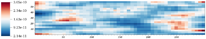
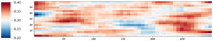
Figure 1: The permeability $\kappa$ [m²] used in the 2D benchmark problem

Figure 2: The porosity $\phi$ used in the 2D benchmark problem

The domain is initially fully saturated with the non-wetting phase ($s_{0}\equiv 0$), which is then displaced by the wetting phase entering from the left boundary, modelled via the boundary conditions

$$\begin{aligned} s&=1.0&\text{in }\Gamma_{s,d}\times[0,T],\\ p&=10&\text{in }\Gamma_{p,d}\times[0,T],\end{aligned}\qquad\begin{aligned} -\lambda(s)\kappa\nabla p\cdot\mathrm{n}&=3\cdot 10^{-4}&\text{in }\Gamma_{p,n}^{1}\times[0,T],\\ -\lambda(s)\kappa\nabla p\cdot\mathrm{n}&=0&\text{in }\Gamma_{p,n}^{2}\times[0,T],\end{aligned}$$

on $\Gamma_{s,d}=\Gamma_{p,d}=\{0\}\times[0,60]$ and $\Gamma_{p,n}=\Gamma_{p,n}^{1}\cup\Gamma_{p,n}^{2}$, where $\Gamma_{p,n}^{1}=\{300\}\times[0,60]$, $\Gamma_{p,n}^{2}=[0,300]\times\{0\}\cup[0,300]\times\{60\}$. In this benchmark no sources are used ($q_{1}\equiv q_{2}\equiv 0.0$) and we neglect gravity so that $G=(0.0,0.0)^{\tau}$. The relative permeabilities in Equation (2) are given here via the linear relations $k_{\text{rw}}(s)=s$ and $k_{\text{ro}}(s)=1-s$ for simplicity. Different relations like the Brooks-Corey or van Genuchten law would be possible. Figure 3 shows the saturation ${s_{h}}$ computed with the full scheme (Algorithm 1) after approximately 3.5, 10, 15, and 48 hours.

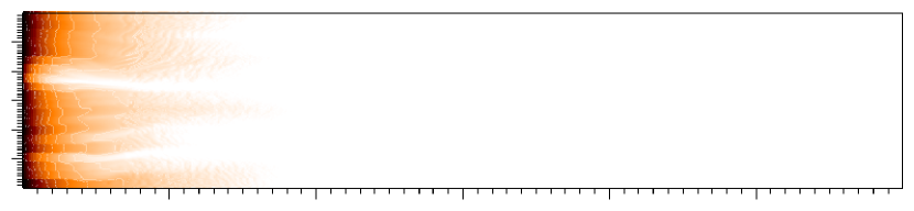
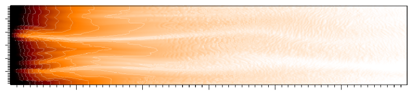
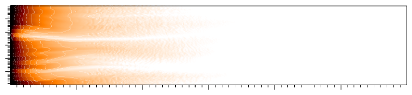
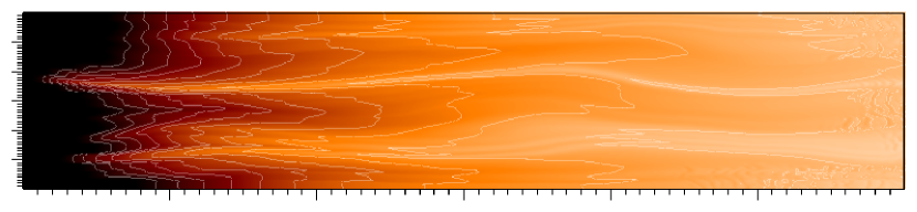
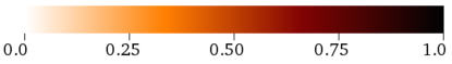
Figure 3: Wetting phase saturation ${s_{h}}$ computed using the LRBMS method after 3.5, 10, 15 and 48 hours (from left to right and top to bottom) including contour lines

From the time-of-flight, which is depicted in Figure 4, we compute eight wetting and non-wetting mobility profiles using Algorithm 2. The resulting wetting mobility profiles are depicted in Figure 5.

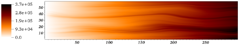
Figure 4: The time-of-flight $\tau^{s}_{h}$ for the 2D benchmark problem for $s=0$

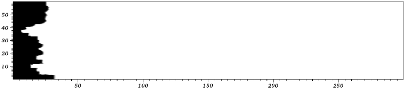
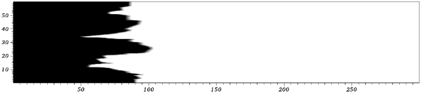
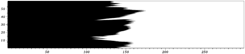
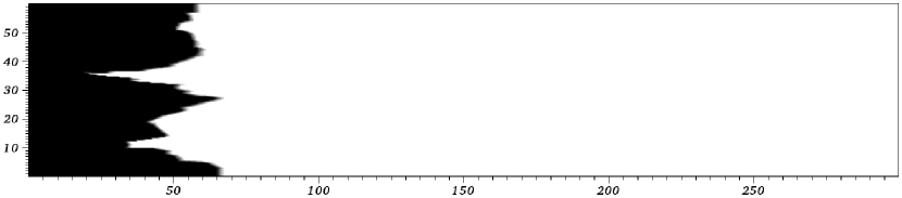
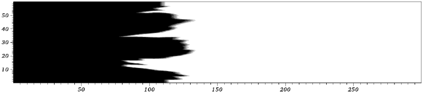
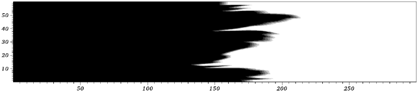
Figure 5: Wetting mobility profiles computed with Algorithm 2 for the time-of-flight depicted in Figure 4. Not shown are the profiles for $q=1$ and $q=M$ which have constant values $\Lambda_{w}^{0}\equiv 0$ and $\Lambda_{w}^{M}\equiv 765.808$, respectively.

Using the profiles we compute the reduced basis $\Phi$ using coarse meshes with sizes $|{\mathcal{T}_{H}}|=1,4,8,16,32$. We use the tolerance $\epsilon_{\text{tol}}=10^{-4}$, a training set $\mathcal{P}_{\text{tr}}$ consisting of $300$ randomly distributed parameters $\mathbf{\mu}$ in $[0.0001,1]^{8}$ with $\sum(\mathbf{\mu})_{i}=1$, and the maximum size $N_{\max}=\infty$ for Algorithm 2. The resulting basis sizes can be seen in Table 1. We observe that with increasing size of the coarse mesh (first column), the number of snapshots computed in Step 2c of Algorithm 2 (fourth column) decreases significantly from 134 to 69. At the same time, the overall basis size (the sum of all local basis sizes, second column) increases. Notice that the basis size is not necessarily equal the product between the number of snapshots and the coarse grid size. This is because we orthonormalize each new snapshot with respect to the existing basis in each extension during the basis generation, reject local extensions with norms below a certain threshold to avoid linear dependencies in the resulting basis and hence reduce the number of local basis functions.

Table 1: Basis sizes $|\Phi|$ resulting from Algorithm 2 for the 2D benchmark problem and a fine triangulation with 64000 elements: Size of the coarse mesh, sum of all local basis sizes before and after application of the PCA, number of snapshots computed during the basis generation

In Table 1 we also see the impact of the local data compression using PCA (Step 3b in Algorithm 2): With increasing coarse mesh size, the PCA is able to reduce the local basis sizes significantly on the different coarse elements.

This effect can be seen again in Figure 6 where we plot the local basis sizes after the PCA step for the test run presented in Table 1, last line. We observe that the local basis size varies strongly from left to right, due to the fact that the peak saturation does not reach the right half of the computational domain before the end time $T$. Also, the basis size differs from bottom to top, especially in regions where the permeability, which is plotted in the background of Figure 6, shows strong variation from bottom to top.

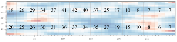
Figure 6: Foreground: local basis sizes after the basis generation performed for Table 1, last line, including the PCA. Background: permeability field

In Tables 2 and 3 we see the resulting discrepancies between the saturation ${s_{h}^{n}}$ computed by the SWIP-DG method on the fine mesh (Algorithm 1) and the saturation ${s_{H}^{n}}$ computed with the reduced scheme 3, as well as the discrepancy between the SWIP-DG pressure and the reduced pressure during the two-phase flow simulation. We present both the relative $L^{2}$ and $H^{1}$ discrepancies for the saturation

$$\Delta_{L^{2}}^{n}=\frac{\|{s_{h}^{n}}-{s_{H}^{n}}\|_{L^{2}(\Omega)}}{\|{s_{h}^{n}}\|_{L^{2}(\Omega)}},\quad\Delta_{H^{1}}^{n}=\frac{\|{s_{h}^{n}}-{s_{H}^{n}}\|_{H^{1}(\Omega)}}{\|{s_{h}^{n}}\|_{H^{1}(\Omega)}},$$

and the respective quantities for the pressure. For different coarse grids, the second column in each table displays the number of snapshots computed during the extension step 2c in Algorithm 2 as a measure for the amount of work needed in that step. Then, in the two sections for the $L^{2}$ and $H^{1}$ relative discrepancies, we present mean discrepancies over all time steps and the discrepancy at the last time step $t^{N_{T}}$ for basis generations without and with usage of the PCA.

Over the different coarse mesh configurations, we consistently observe a mean $L^{2}$-discrepancy for the saturation of approximately $5.6$% (standard deviation: $1.6$%), both with and without the PCA, which is reduced to $4.3$% at end time. The respective $H^{1}$-discrepancies are slightly bigger with a mean of $7.9$% (standard deviation: $2.9$%) and $5.5$% at end time. The mean $L^{2}$-discrepancy for the pressure is approximately $1.4$% (standard deviation: $0.3$%) for all coarse grid configurations, and reduces to $1.3$% at end time. The respective $H^{1}$-discrepancies are in the same ranges. In conclusion, we can say that the data compression step using the PCA increases neither the error for the pressure nor the error for the saturation noticeably.

While we can ensure mass conservation on the coarse grid by adding per-coarse-cell unit basis functions to the reduced basis, the method is not mass-conservative on the fine grid. In Figure 7 we plot the relative mass loss

$$\zeta^{n}:{\mathcal{T}_{h}}\to\mathbb{R}^{+},\quad\zeta^{n}(e)=\frac{1}{\max_{x\in\partial e}\|{u_{h}^{n}}(x)\|_{l^{2}}}\left|\int_{\partial e}{u_{h}^{n}}\cdot\mathrm{n}\,\mathrm{d}S\right|$$

as a measure of the lack of mass conservation at end time $t^{n}=3\cdot 10^{5}$ for the velocity computed with the LRBMS scheme on a $16\times 2$ coarse grid. We see that the velocity lacks mass conservation mainly on coarse cell intersections and in regions with large gradients in the mobility profiles $\Lambda^{i}$. Overall, the relative lack of mass conservation is well below $2\cdot 10^{-5}$. Although we therefore found this to be only a minor problem in the tests—the saturation usually did not grow above a value of $1.05$ and hardly ever fell below zero—future work will include research on how to ensure mass-conservation on the fine grid.

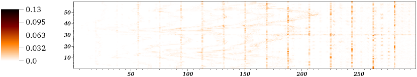
Figure 7: Relative mass loss $\zeta^{n}$ for the final time step $t^{n}=3\cdot 10^{5}$

As the discrepancies are increased neither by introducing more coarse cells, nor by application of the PCA, we find the Localized Reduced Basis Multiscale method to be well applicable in this context: Introduction of more coarse cells reduces the number of costly snapshots to be computed during the basis construction, while application of the PCA yields smaller, more compact bases, leading to faster computations during the two-phase flow simulation.

Table 2: Relative $L^{2}$ and $H^{1}$ discrepancies between the saturation computed with Algorithm 3 and the saturation computed with the fine-scale algorithm 1 for different coarse mesh configurations: Number of snapshots needed during the basis construction, mean relative $L^{2}$ discrepancy and relative $L^{2}$ discrepancy at end time $T$ without using the PCA, respective quantities after usage of the PCA, respective quantities for the $H^{1}$ norm

Table 3: Relative $L^{2}$ and $H^{1}$ discrepancies between the pressure computed with Algorithm 3 and the pressure computed with the fine-scale algorithm 1 for different coarse mesh configurations: Number of snapshots needed during the basis construction, mean relative $L^{2}$ discrepancy and relative $L^{2}$ discrepancy at end time $T$ without using the PCA, respective quantities after usage of the PCA, respective quantities for the $H^{1}$ norm

Test runs with a different tolerance $\epsilon_{\text{tol}}=10^{-5}$ for the Greedy basis construction (Algorithm 2) exhibit the same discrepancies in both the $L^{2}$ and $H^{1}$ norms. Further, computations with higher numbers of mobility profiles ($M=10,12,20$) give roughly the same discrepancies. This gives rise to the assumption that the error is dominated by different phenomena, which we consider to be twofold: First, the assumption that the time-of-flight is invariant for the whole simulation is not valid in some regions. Therefore, the position of the saturation front and its impact on the mobility cannot be represented correctly. Second, the profile of the mobility along streamlines is not approximated well enough due to the ad-hoc profile generation in Algorithm 2.

To support the first statement, we present in Figure 8 the absolute value of the difference between the SWIP-DG approximation ${s_{h}^{N_{T}}}$ and our approximation of the saturation ${s_{H}^{N_{T}}}$ at end time $t^{N_{T}}$. We see that huge discrepancies arise in three distinct positions: around the point $\mathbf{x}=(30,35)$, the point $\mathbf{x}=(40,10)$, and the point $\mathbf{x}=(80,1)$. These positions are located directly downwind along the streamlines from points where the time-of-flight changes significantly during the test run, see Figure 9. The error produced in those regions is then transported through the domain along the streamlines, hence the error distribution to be seen in Figure 8 is established.

The second statement can be justified by using $M$ high-dimensional saturation approximations ${s_{h}^{n_{1}}},\ldots,{s_{h}^{n_{M}}}$ at points $t^{1},\ldots,t^{M}$ in time to form the profiles in Step 1c of Algorithm 2:

$$\Lambda_{w}^{q}=\lambda_{w}({s_{h}^{q}}),\quad\Lambda_{o}^{q}=\lambda_{o}({s_{h}^{q}}).$$

In doing so, we ensure that the shape of the mobility profiles along streamlines is correct and the error of the LRBMS two-phase flow scheme should decrease drastically. Indeed, for $M=8$, this procedure decreases the mean relative $L^{2}$-discrepancy to 2.3% with a standard deviation of 2.0%. Even more: The $L^{2}$-discrepancy at $t=T$ is reduced by a factor of ten to 0.45%. Obviously, using multiple high-dimensional saturation profiles is not possible in general as the model order reduction would become superfluous, but two other remedies could be implemented: One could be to recompute the mobility profiles and the reduced basis after a certain number of time steps $t^{n}$ using the time-of-flight for ${s_{h}^{n}}$. Another approach could be to solve the full high-dimensional two-phase flow problem along some streamlines in one dimension in a preparatory step and use a combination of the resulting mobility profiles as a replacement for those in Step 1c of Algorithm 2.

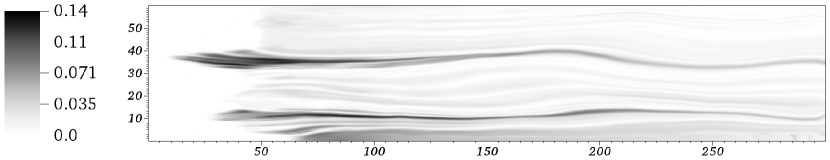
Figure 8: Absolute value of the difference in the saturation ${s_{h}^{N_{T}}}$ computed with the full high-dimensional scheme and the saturation ${s_{H}^{N_{T}}}$ computed with the LRBMS scheme at end time $T$

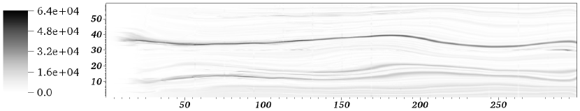
Figure 9: Absolute difference between the time-of-flight for the initial saturation $s_{0}$ and the time-of-flight for the saturation computed with the LRBMS scheme for a coarse grid with $16\times 2$ cells at time $t=10000s$

In Table 4 we present runtimes for the basis construction part of the LRBMS two-phase flow scheme. Again, we give the coarse grid configuration (column one) and the number of snapshots needed (column two). The third column then shows the time needed for the basis construction (Algorithm 2). The timings presented here include the time for the computation of the mobility profiles (about 13 seconds), the so-called “training”-step (computation of all reduced solutions, evaluation of the error measure, selection of the parameter for basis extension), and the extension-step including the computation of a high-dimensional snapshot and application of the Gram-Schmidt procedure. It does not contain the application of the PCA which is consistently below one second for all coarse grid configurations and hence can be considered negilgible. The time needed to compute the reduced basis $\Phi$ is 50 minutes on one coarse cell (which corresponds to a standard Reduced Basis method), goes up to 1 hour 7 minutes for a coarse grid of size $4\times 1$ and is then reduced to 45 minutes for all other coarse grids. The increase in total runtime from line one to line two can explained by the relatively high number of iterations that is still needed to reach the error tolerance with an increased per-step cost due to the larger reduced bases. This effect would vanish if the snapshot computation (column four) was more expensive, for larger fine grids, for example. As mentioned earlier, we use the true error as error measure. The time for error estimation in column five includes the time needed to reconstruct a high-dimensional snapshot from each reduced solution and compute the difference in the $L^{2}$-norm. The time for computation of the high-dimensional snapshots itself is not included.

In conclusion we can say that for the test case at hand, introduction of more coarse cells yields slight reductions in terms of runtime. As the computation of the snapshots shows a speedup by a factor of two for the computation on 32 coarse cells compared to the computation on one coarse cell, we can expect the runtime-gain to increase drastically as the size of the fine mesh—and hence the time for the computation of one high-dimensional snapshot—is increased.

Table 4: Runtimes for the basis construction (Algorithm 2): Coarse grid size, number of snapshots computed, total runtime, total time for snapshot computation, total time for error estimation

Finally, in Table 5 we present runtimes for the two-phase flow simulation (Step 5 in Algorithm 3) for uncompressed bases (that is: bases that were computed without usage of the PCA) and compressed bases on different coarse grids and, for comparison, the same runtimes for a full high-dimensional computation. We see that for the reduced simulations, more than 50% of the overall runtime of about 2 hours 40 minutes is spend in the application of the ODE solver and slope limiter for the saturation equation. About one hour is spend for the elliptic equation with about 45 minutes for the reconstruction of the flux (see Definition 2). For uncompressed bases, computing all pressure solutions takes five to 15 minutes, depending on the coarse grid and respective basis size, for compressed bases those times drop to two to five minutes.

The time to solution for one reduced pressure computation therefore ranges from 20 milliseconds on the $1\times 1$, $4\times 1$ and $8\times 1$ coarse grids to 50 milliseconds on the $8\times 2$ and $16\times 2$ coarse grids using the PCA. Comparing these runtimes to the time needed for a high-dimensional simulation we see the advantage of our method: The high-dimensional test run takes approximately 16 hours with nearly 90% of the time spent in the treatment of the elliptic equation: more than two hours are spent assembling the pressure system, solving it takes approximatly 11 hours in total (approximately seven seconds per solve). The speed-up for the solution of the pressure equation is approximately a factor 140. Because nothing was done to speed up the transport solve, the overall speed-up for the two-phase flow simulation (high-dimensional vs. basis construction and reduced simulation) is five. To also speed up the transport solve significantly, one could replace the explicit temporal discretization by a backward Euler scheme and utilize the fact that the resulting nonlinear system share the same unidirectional flow properties as the time-of-flight equation and hence can be computed in a per-element fashion with local control over the nonlinear iterations; see [53] for details. Note that in this case, the slope limiter presented in Section 3 needs to be replaced by a different kind of stabilization as it is not compliant with implicit time stepping schemes.

Table 5: Runtimes for Step 5 of Algorithm 3 for uncompressed and compressed bases: Coarse grid size, total runtime, time spent for treatment of the elliptic equation, thereof time spent in pressure solve and velocity reconstruction and time spent in saturation part. Last line: same numbers for a full high-dimensional simulation

7 Summary and Outlook

We introduced a localized version of the Reduced Basis method. The idea of our approach is to make use of two computational meshes: A fine mesh is used to compute detailed solutions of a parametrized elliptic equation for different parameters. Those solutions are then localized to the cells of a second, coarser mesh. An optional data compression is applied and the result is used as basis for a reduced-dimensional surrogate of the high-dimensional scheme. We applied this technique to the pressure equation in a two-phase flow setting replacing the orignal mobility by a parametrized approximation. We were able to demonstrate significant reduction of the computational effort at acceptable error compared to a full detailed two-phase flow simulation.

The quality of the reduced approximations for saturation and pressure is mainly decided by the quality of the approximation of the original mobility by our parametrized surrogate, therefore future work will include improvements of the mobility approximation.

Mass conservation can only be guaranteed on the coarse mesh of our scheme, in future work we will address the problem of mass conservation on the fine mesh for the reduced simulations. Applying the LRBMS to the saturation equation also would be an extension promising additional speedup.

References

- [1] Farmer CL. Upscaling: a review. Int. J. Numer. Meth. Fluids 2002; 40(1–2):63–78, 10.1002/fld.267.
- [2] Durlofsky LJ. Upscaling and gridding of fine scale geological models for flow simulation 2005. Presented at 8th International Forum on Reservoir Simulation Iles Borromees, Stresa, Italy, June 20–24, 2005.
- [3] Hughes TJR. Multiscale phenomena: Green’s functions, the Dirichlet-to-Neumann formulation, subgrid scale models, bubbles and the origins of stabilized methods. Comput. Methods Appl. Mech. Engrg. 1995; 127(1-4):387–401.
- [4] Efendiev Y, Hou TY. Multiscale Finite Element Methods, Surveys and Tutorials in the Applied Mathematical Sciences, vol. 4. Springer Verlag, 2009.
- [5] Hughes TJR, Feijóo GR, Mazzei L, Quincy JB. The variational multiscale method—a paradigm for computational mechanics. Comput. Methods Appl. Mech. Engrg. 1998; 166(1-2):3–24.
- [6] Hou TY, Wu XH. A multiscale finite element method for elliptic problems in composite materials and porous media. J. Comput. Phys. 1997; 134(1):169–189.
- [7] Efendiev Y, Galvis J, Hou TY. Generalized Multiscale Finite Element Methods (GMsFEM). arXiv.org Jan 2013; URL http://arxiv.org/abs/1301.2866v2.
- [8] Chen Z, Hou TY. A mixed multiscale finite element method for elliptic problems with oscillating coefficients. Math. Comput. 2003; 72(242):541–576.
- [9] Aarnes JE, Krogstad S, Lie KA. Multiscale mixed/mimetic methods on corner-point grids. Computational Geosciences Jan 2008; 12(3):297–315, 10.1007/s10596-007-9072-8. URL http://www.springerlink.com/index/10.1007/s10596-007-9072-8.
- [10] Arbogast T. Implementation of a locally conservative numerical subgrid upscaling scheme for two-phase Darcy flow. Comput. Geosci. 2002; 6(3-4):453–481.
- [11] Arbogast T, Pencheva G, Wheeler MF, Yotov I. A multiscale mortar mixed finite element method. Multiscale Model. Sim. 2007; 6(1):319–346.
- [12] Jenny P, Lee SH, Tchelepi H. Multi-scale finite-volume method for elliptic problems in subsurface flow simulations. Journal of Computational Physics 2003; 187:47–67.
- [13] Møyner O, Lie KA. A multiscale two-point flux-approximation method. J. Comput. Phys 2014; .
- [14] Henning P, Ohlberger M, Schweizer B. Adaptive Heterogeneous Multiscale Methods for immiscible two-phase flow in porous media. Multiple values selected Jul 2013; URL http://arxiv.org/abs/1307.2123.
- [15] E W, Engquist B. The heterogeneous multiscale methods. Commun. Math. Sci. 2003; 1(1):87–132.
- [16] Peterseim D, Henning P, Morgenstern P. Multiscale Partition of Unity. arXiv.org Dec 2013; URL http://arxiv.org/abs/1312.5922.
- [17] Prud’homme C, Rovas DV, Veroy K, Patera AT. A mathematical and computational framework for reliable real-time solution of parametrized partial differential equations. M2AN. Mathematical Modelling and Numerical Analysis 2002; 36(5):747–771, 10.1051/m2an:2002035. URL http://dx.doi.org/10.1051/m2an:2002035.
- [18] Machiels L, Maday Y, Oliveira IB, Patera AT, Rovas DV. Output bounds for reduced-basis approximations of symmetric positive definite eigenvalue problems. Comptes Rendus de l’Académie des Sciences Série I Mathématique 2000; 331(2):153–158, 10.1016/S0764-4442(00)00270-6. URL http://dx.doi.org/10.1016/S0764-4442(00)00270-6.
- [19] Prud’homme C, Rovas DV, Veroy K, Machiels L, Maday Y, Patera AT, Turinici G. Reliable real-time solution of parametrized partial differential equations: Reduced-basis output bound methods. Journal of Fluids Engineering-Transactions of the Asme Mar 2002; 124(1):70–80, 10.1115/1.1448332. URL http://augustine.mit.edu/methodology/papers/atpJFE2002.pdf.
- [20] Patera AT, Rozza G. Reduced Basis Approximation and a Posteriori Error Estimation for Parametrized Partial Differential Equations. Version 1.0, Copyright MIT 2006, to appear in (tentative rubric) MIT Pappalardo Graduate Monographs in Mechanical Engineering 2006; .
- [21] Nguyen NC, Veroy K, Patera AT. Certified Real-Time Solution of Parametrized Partial Differential Equations. Handbook of Materials Modeling. Springer Netherlands: Dordrecht, 2005; 1529–1564, 10.1007/978-1-4020-3286-8_76. URL http://link.springer.com/10.1007/978-1-4020-3286-8_76.
- [22] Grepl MA, Patera AT. A posteriori error bounds for reduced-basis approximations of parametrized parabolic partial differential equations. M2AN. Mathematical Modelling and Numerical Analysis 2005; 39(1):157–181, 10.1051/m2an:2005006. URL http://journals.cambridge.org/abstract_S0764583X05000063.
- [23] Rovas DV, Machiels L, Maday Y. Reduced-basis output bound methods for parabolic problems. Ima Journal of Numerical Analysis Jul 2006; 26(3):423–445, 10.1093/imanum/dri044. URL http://dx.doi.org/10.1093/imanum/dri044.
- [24] Grepl MA, Maday Y, Nguyen NC, Patera AT. Efficient reduced-basis treatment of nonaffine and nonlinear partial differential equations. M2AN. Mathematical Modelling and Numerical Analysis 2007; 41(3):575–605, 10.1051/m2an:2007031. URL http://dx.doi.org/10.1051/m2an:2007031.
- [25] Haasdonk B, Ohlberger M. Reduced basis method for finite volume approximations of parametrized linear evolution equations. M2AN. Mathematical Modelling and Numerical Analysis 2008; 42(2):277–302, 10.1051/m2an:2008001. URL http://dx.doi.org/10.1051/m2an:2008001.
- [26] Haasdonk B, Ohlberger M, Rozza G. A Reduced Basis Method for Evolution Schemes with Parameter-Dependent Explicit Operators. Electronic Transactions on Numerical Analysis 2008; 32:145–161. URL http://www.emis.ams.org/journals/ETNA/vol.32.2008/pp145-161.dir/pp145-161.pdf.
- [27] Haasdonk B, Ohlberger M. Reduced basis method for explicit finite volume approximations of nonlinear conservation laws. Hyperbolic problems: theory, numerics and applications. Amer. Math. Soc.: Providence, RI, 2009; 605–614. URL http://www.ams.org/mathscinet-getitem?mr=MR2605256.
- [28] Drohmann M, Haasdonk B, Ohlberger M. Reduced Basis Model Reduction of Parametrized Two-Phase Flow in Porous Media. MATHMOD 2012 - 7th Vienna International Conference on Mathematical Modelling, Vienna, February 15 - 17, 2012, 2012.
- [29] Veroy K, Prud’homme C, Rovas DV, Patera AT. A Posteriori Error Bounds for Reduced-Basis Approximation of Parametrized Noncoercive and Nonlinear Elliptic Partial Differential Equations. 16th AIAA Computational Fluid Dynamics Conference, American Institute of Aeronautics and Astronautics: Orlando, Florida, 2003, 10.2514/6.2003-3847. URL http://arc.aiaa.org/doi/abs/10.2514/6.2003-3847.
- [30] Barrault M, Maday Y, Nguyen NC, Patera AT. An ’empirical interpolation’ method: application to efficient reduced-basis discretization of partial differential equations. Comptes Rendus Mathematique Oct 2004; 339(9):6–6, 10.1016/j.crma.2004.08.006. URL http://dx.doi.org/10.1016/j.crma.2004.08.006.
- [31] Drohmann M, Haasdonk B, Ohlberger M. Reduced basis approximation for nonlinear parametrized evolution equations based on empirical operator interpolation. SIAM Journal on Scientific Computing 2012; 34(2):A937–A969, 10.1137/10081157X. URL http://dx.doi.org/10.1137/10081157X.
- [32] Kaulmann S, Ohlberger M, Haasdonk B. A new local reduced basis discontinuous Galerkin approach for heterogeneous multiscale problems. Comptes Rendus Mathematique Dec 2011; 349(23-24):1233–1238, 10.1016/j.crma.2011.10.024. URL http://www.sciencedirect.com/science/article/pii/S1631073X11003074.
- [33] Albrecht F, Haasdonk B, Kaulmann S, Ohlberger M. The Localized Reduced Basis Multiscale Method. Algoritmy 2012, Handlovičová A, Minarechová Z, Ševčovič D (eds.), Slovak University of Technology in Bratislava, Publishing House of STU, 2012; 393–403. URL http://www.simtech.uni-stuttgart.de/publikationen/prints.php?ID=698.
- [34] Schindler F, Ohlberger M. A-posteriori error estimates for the localized reduced basis multi-scale method. arXiv.org Jan 2014; URL http://arxiv.org/abs/1401.7173.
- [35] Smetana K. A new certification framework for the port reduced static condensation reduced basis element method. Submitted to Computer Methods in Applied Mechanics and Engineering Mar 2014; .
- [36] Ern A, Mozolevski I, Schuh L. Discontinuous Galerkin approximation of two-phase flows in heterogeneous porous media with discontinuous capillary pressures. Computer Methods in Applied Mechanics and Engineering Apr 2010; 199(23-24):11–11, 10.1016/j.cma.2009.12.014. URL http://dx.doi.org/10.1016/j.cma.2009.12.014.
- [37] Rivière B. Discontinuous Galerkin Methods for Solving Elliptic and Parabolic Equations. Theory and Implementation, SIAM, 2008. URL http://dx.doi.org/10.1137/1.9780898717440.
- [38] Dedner A, Klöfkorn R. A Generic Stabilization Approach for Higher Order Discontinuous Galerkin Methods for Convection Dominated Problems - Springer. Journal of Scientific Computing 2011; 47(3). URL http://link.springer.com/article/10.1007/s10915-010-9448-0.
- [39] Natvig JR, Lie KA, Eikemo B, Berre I. A discontinuous Galerkin method for computing single-phase flow in porous media. Adv Water Resour 2007; URL http://heim.ifi.uio.no/~kalie/papers/dg-tof.pdf.
- [40] Knezevic D, Huynh DBP, Patera AT. A static condensation reduced basis element method: approximation and a posteriori error estimation. ESAIM: Mathematical Modelling and Numerical Analysis Sep 2012; -1(-1):–, 10.1051/m2an/2012022. URL http://www.esaim-m2an.org/10.1051/m2an/2012022.
- [41] Maday Y, Rønquist EM. The reduced basis element method: Application to a thermal fin problem. SIAM Journal on Scientific Computing 2004; 26(1):240–258, 10.1137/S1064827502419932. URL http://dx.doi.org/10.1137/S1064827502419932.
- [42] Chen Y, Hesthaven JS, Maday Y. A Seamless Reduced Basis Element Method for 2D Maxwell’s Problem: An Introduction. Lecture Notes in Computational Science and Engineering1439-7358, Hesthaven JS, Rønquist EM (eds.). Springer Berlin Heidelberg: Berlin, Heidelberg, 2010; 141–152, 10.1007/978-3-642-15337-2_11. URL http://www.springerlink.com/index/10.1007/978-3-642-15337-2_11.
- [43] Iapichino L, Quarteroni A, Rozza G. A reduced basis hybrid method for the coupling of parametrized domains represented by fluidic networks. Computer Methods in Applied Mechanics and Engineering 2012; 221:63–82, 10.1016/j.cma.2012.02.005. URL http://dx.doi.org/10.1016/j.cma.2012.02.005.
- [44] Iapichino L. Reduced Basis Methods for the Solution of Parametrized PDEs in Repetitive and Complex Networks with Application to CFD. PhD Thesis, École Polytechnique Fédérale de Lausanne, Lausanne Oct 2012.
- [45] Maier I, Rozza G, Haasdonk B. Reduced basis approximation and a-posteriori error estimation for the coupled Stokes-Darcy system. Simtech Preprint 2014, University of Stuttgart 2014; URL http://www.simtech.uni-stuttgart.de/publikationen/prints.php?ID=848.
- [46] Chaturantabut S, Sorensen DC. Application of POD and DEIM on dimension reduction of non-linear miscible viscous fingering in porous media. Mathematical and Computer Modelling of Dynamical Systems Aug 2011; 17(4):337–353, 10.1080/13873954.2011.547660. URL http://www.tandfonline.com/doi/abs/10.1080/13873954.2011.547660.
- [47] Krogstad S. A sparse basis POD for model reduction of multiphase compressible flow. SPE Reservoir Simulation Symposium, The Woodlands, TX, USA, 21–23 February 2011, 2011, 10.2118/141973-MS. SPE 141973-MS.
- [48] Jolliffe IT. Principal Component Analysis. Springer, 2002. URL http://www.springer.com/statistics/statistical+theory+and+methods/book/978-0-387-95442-4.
- [49] Bastian P, Blatt M, Dedner A, Engwer C, Klöfkorn R, Ohlberger M, Sander O. A generic grid interface for parallel and adaptive scientific computing. I. Abstract framework. Computing 2008; 82(2-3):103–119, 10.1007/s00607-008-0003-x. URL http://dx.doi.org/10.1007/s00607-008-0003-x.
- [50] Bastian P, Blatt M, Dedner A, Engwer C, Klöfkorn R, Kornhuber R, Ohlberger M, Sander O. A generic grid interface for parallel and adaptive scientific computing. Part II: Implementation and Tests in DUNE. Computing Jun 2008; 82(2-3):121–138, 10.1007/s00607-008-0004-9. URL http://www.springerlink.com/index/10.1007/s00607-008-0004-9.
- [51] Dedner A, Klöfkorn R, Nolte M, Ohlberger M. A generic interface for parallel and adaptive discretization schemes: abstraction principles and the Dune-Fem module. Computing Aug 2010; 90(3-4):165–196, 10.1007/s00607-010-0110-3. URL http://www.springerlink.com/index/10.1007/s00607-010-0110-3.
- [52] Dedner A, Flemisch B, Klöfkorn R ( (eds.)). Advances in DUNE: Proceedings of the DUNE User Meeting, Held in October 6th-8th 2010 in Stuttgart, Germany. 2012 edn., Springer, 2012. URL http://dx.doi.org/10.1007/978-3-642-28589-9.
- [53] Natvig JR, Lie KA. Fast computation of multiphase flow in porous media by implicit discontinuous Galerkin schemes with optimal ordering of elements. J. Comput. Phys. 2008; 227(24):10 108–10 124, 10.1016/j.jcp.2008.08.024. URL http://dx.doi.org/10.1016/j.jcp.2008.08.024.