Distributed Compressive CSIT Estimation and Feedback for FDD Multi-user Massive MIMO Systems

Abstract

To fully utilize the spatial multiplexing gains or array gains of massive MIMO, the channel state information must be obtained at the transmitter side (CSIT). However, conventional CSIT estimation approaches are not suitable for FDD massive MIMO systems because of the overwhelming training and feedback overhead. In this paper, we consider multi-user massive MIMO systems and deploy the compressive sensing (CS) technique to reduce the training as well as the feedback overhead in the CSIT estimation. The multi-user massive MIMO systems exhibits a hidden joint sparsity structure in the user channel matrices due to the shared local scatterers in the physical propagation environment. As such, instead of naively applying the conventional CS to the CSIT estimation, we propose a distributed compressive CSIT estimation scheme so that the compressed measurements are observed at the users locally, while the CSIT recovery is performed at the base station jointly. A joint orthogonal matching pursuit recovery algorithm is proposed to perform the CSIT recovery, with the capability of exploiting the hidden joint sparsity in the user channel matrices. We analyze the obtained CSIT quality in terms of the normalized mean absolute error, and through the closed-form expressions, we obtain simple insights into how the joint channel sparsity can be exploited to improve the CSIT recovery performance.

I Introduction

Massive multiple-input multiple-output (MIMO) can greatly enhance the wireless communication capacity due to the increased degrees of freedom [1], and there is intense research interest in the applications of massive MIMO in next generation wireless systems [2]. To fully utilize the spatial multiplexing gains and the array gains of massive MIMO [3, 4], knowledge of channel state information at the transmitter (CSIT) is essential. In time-division duplexing (TDD) massive MIMO systems, the CSIT can be obtained by exploiting the channel reciprocity using uplink pilots [5] and hence, lots of works today [2, 6] have considered massive MIMO of TDD systems. On the other hand, as frequency-division duplexing (FDD) is generally considered to be more effective for systems with symmetric traffic and delay-sensitive applications [7] and the most cellular systems today employ FDD, it is therefore of great interest to explore effective approaches for obtaining CSIT for massive MIMO with FDD [8]. To obtain CSIT at the base station (BS) of FDD systems, the BS first transmits downlink pilot symbols so that the user can estimate the downlink CSI locally. The estimated CSI are then fed back to the BS via uplink signaling channels [9]. Conventional methods to estimate the downlink CSI at the users include least square (LS) [10] and minimum mean square error (MMSE) [11]. However, using these conventional CSI estimation techniques, the number of independent pilot symbols required at the BS has to scale linearly with the number of transmit antennas $M$ at the BS (i.e. $O(M)$). For massive MIMO, as $M$ becomes very large, the pilot training overhead (downlink) as well as the CSI feedback overhead (uplink) would be prohibitively large. In addition, the number of independent pilot symbols available is limited by the channel coherence time and coherence bandwidth [2], as illustrated in Figure 1. Obviously, as $M$ increases in FDD massive MIMO systems, we do not have sufficient pilots to support CSIT estimation despite the overhead issues. Hence, a new CSIT estimation and feedback design will be needed to support FDD massive MIMO systems.

There is one important observation for massive MIMO systems, which can help to address the above issues. From many experimental studies of massive MIMO channels [12, 13, 14, 15, 16], as $M$ increases, the user channel matrices tend to be sparse due to the limited local scatterers at the BS. Hence, it is very inefficient to estimate the entire CSI matrices using long pilot training symbols at the BS. Instead, we should exploit the hidden sparsity in the CSIT estimation and feedback process and compressive sensing (CS) is an attractive framework for this purpose [17]. In fact, the CS techniques have already been used in the literature to enhance the channel estimation performance. For instance, in [6], a CS-based low-rank approximation algorithm is proposed to enhance the channel estimation performance for TDD massive MIMO systems but the technique cannot be applied for FDD systems. In [18], a CS-based channel estimation method is proposed to exploit the per-link sparse multipath channels in time, frequency as well as spatial domains in MIMO systems. By exploiting the spatial sparsity using CS in massive MIMO systems, it is shown that only $O(s\log M)$ training overhead [18] is needed and this represents a substantial reduction of the CSIT estimation overhead compared with the conventional LS approach. To extend existing CS-based CSIT estimation techniques to multi-user massive MIMO of FDD systems, we need to address several first order technical challenges:

• How to exploit the joint channel sparsity among different users distributively. As has been observed in many experimental studies [14, 13, 15, 16], the user channel matrices of a multi-user massive MIMO system may be jointly correlated due to the shared common local scattering clusters [19]. Therefore, it is highly desirable to exploit not only the per-link channel sparsity but also the joint sparsity structure to further reduce the CSIT estimation and feedback overhead. Directly applying existing CS-based CSIT estimation for point to point links [18, 17, 20] may exploit the per-link channel sparsity, but it fails to exploit the joint sparsity in the user channel matrices. In [21], the authors consider a distributed CS recovery framework based on three simple joint sparsity models. A set of jointly sparse signal ensembles are measured distributively and recovered jointly. However, the joint sparsity structure in our multi-user massive MIMO scenario is much more complicated and is not covered by these existing models [21] and hence, the associated recovery algorithms cannot be extended to our scenario.

• Tradeoff analysis between the CSIT estimation quality and the joint channel sparsity. Besides the algorithm development challenge above, it is also desirable to obtain design insights into how the joint channel sparsity can affect the CSIT estimation performance. However, in general, the performance analysis of the joint CS recovery algorithms is very difficult [22]. In [23, 24], the authors analyze the support recovery probability of the simultaneous orthogonal matching pursuit algorithm proposed for multiple measurement vector problems [22], and demonstrate the performance benefits of exploiting the shared sparsity support. However, the analytical approach cannot be easily extended to our scenario as the recovery performance analysis is usually algorithm-specific.

Figure 1: Frame structure with pilot training to obtain CSIT in massive MIMO FDD system.

In this paper, we propose a novel CSIT estimation and feedback method for multi-user massive MIMO FDD systems. The proposed solution autonomously exploits the hidden joint channel sparsity among the users surrounded by some common local scattering clusters [19] to substantially reduce the CSIT estimation and feedback overhead. We first propose a joint sparsity model to incorporate the sparsity features of the channel matrices in multi-user massive MIMO systems. Based on this model, a distributed compressive CSIT estimation and feedback framework is then developed such that the users obtain compressed channel observations locally and feedback these compressed measurements to the BS. CSIT reconstruction is performed at the BS using a joint recovery algorithm based on the fedback compressed measurements. Specifically, we propose, in Section III, a joint orthogonal matching pursuit algorithm to exploit the joint channel sparsity in the CSIT recovery at the BS. We analyze the normalized mean absolute error of the estimated CSI in Section IV, and from the closed-form results, we obtain important insights regarding the role of individual and distributed joint channel sparsity in multi-user massive MIMO systems. Numerical results in Section V demonstrate that the proposed CSIT recovery algorithm can achieve substantial performance gains over conventional LS-based [10, 11] or existing CS-based per-link CSIT estimation solutions [18, 17, 20].

Notations: Uppercase and lowercase boldface denote matrices and vectors respectively. The operators $(\cdot)^{T}$, $(\cdot)^{*}$, $(\cdot)^{H}$, $(\cdot)^{\dagger}$, $|\cdot|$, $I_{\{\cdot\}}$, $\left\lfloor\cdot\right\rfloor$, $\left\lceil\cdot\right\rceil$, $O(\cdot)$, $o(\cdot)$ and $\textrm{Pr}(\cdot)$ are the transpose, conjugate, conjugate transpose, Moore-Penrose pseudoinverse, cardinality, indicator function, round down integer, round up integer, big-O notation, little-o notation, and probability operator respectively; $\textrm{supp}(\mathbf{h})$ is the index set of the non-zero entries of vector $\mathbf{h}$; $\mathbf{A}(l)$, $\mathbf{a}(l)$ and $\mathbf{a}_{\Omega}$ denotes the $l$-th column vector of $\mathbf{A}$, $l$-th entry of $\mathbf{a}$, and sub-vector formed by collecting the entries of $\mathbf{a}$ whose indexes are in set $\Omega$ respectively; $\mathbf{A}_{\Omega}$ and $\mathbf{A}^{\Omega}$ denote the sub-matrices formed by collecting the columns and rows, respectively, of $\mathbf{A}$ whose indexes are in set $\Omega$; $||\mathbf{A}||_{F}$, $||\mathbf{A}||$ and $||\mathbf{a}||$ denote the Frobenius norm, spectrum norm of $\mathbf{A}$ and Euclidean norm of vector $\mathbf{a}$ respectively; denote $[M]=\{1,2,\cdots,M\}$.

II System Model

II-A Multi-user Massive MIMO System

Consider a flat block-fading multi-user massive MIMO system operating in FDD mode. There is one BS and $K$ users in the network as illustrated in Figure 2, where the BS has $M$ antennas ($M$ is large) and each user has $N$ antennas. There is a common downlink pilot channel from the BS in which the BS broadcasts a sequence of $T$ training pilot symbols on its $M$ antennas, as illustrated in Figure 2. Denote the transmitted pilot signal from the BS in the $j$-th time slot as $\mathbf{x}_{j}\in\mathbb{C}^{M\times 1}$, $j=1,\cdots,T$. The received signal vector at the $i$-th user in the $j$-th time slot $\mathbf{y}_{ij}\in\mathbb{C}^{N\times 1}$ can be expressed as

$$\mathbf{y}_{ij}=\mathbf{H}_{i}\mathbf{x}_{j}+\mathbf{n}_{ij},j=1,\cdots,T,$$ (1)

where $\mathbf{H}_{i}\in\mathbb{C}^{N\times M}$ is the quasi-static channel matrix from the BS to the $i$-th user and $\mathbf{n}_{ij}\in\mathbb{C}^{N\times 1}$ is the complex Gaussian noise with zero mean and unit variance. Let $\mathbf{X}=\left[\begin{array}[]{ccc}\mathbf{x}_{1}&\cdots&\mathbf{x}_{T}\end{array}\right]\in\mathbb{C}^{M\times T}$, $\mathbf{Y}_{i}=\left[\begin{array}[]{ccc}\mathbf{y}_{1}&\cdots&\mathbf{y}_{T}\end{array}\right]\in\mathbb{C}^{N\times T}$ and $\mathbf{N}_{i}=\left[\begin{array}[]{ccc}\mathbf{n}_{i1}&\cdots&\mathbf{n}_{iT}\end{array}\right]\in\mathbb{C}^{N\times T}$ be the concatenated transmitted pilots, received signal, and noise vectors respectively; the signal model (1) can be equivalently written as

$$\mathbf{Y}_{i}=\mathbf{H}_{i}\mathbf{X}+\mathbf{N}_{i},$$ (2)

where $\textrm{tr}(\mathbf{X}\mathbf{X}^{H})=PT$ is the sum transmit SNR in the $T$ training time slots and $P$ is the transmit SNR per time slot at the BS.

In order to effectively exploit the array gain and the spatial degrees of freedom in massive MIMO, it is important to obtain CSIT at the BS [3, 4]. For FDD systems, the CSIT knowledge at the BS is obtained by two steps: (i) local CSI estimation of $\mathbf{H}_{i}$ at the $i$-th user and (ii) feedback of the estimated CSI $\mathbf{\hat{H}}_{i}$ to the BS, as illustrated in Figure 1. Using conventional LS-based CSI estimation techniques [10, 25], the LS channel estimate $\mathbf{\hat{H}}_{i}$ is given by

$$\mathbf{\hat{H}}_{i}=\mathbf{Y}_{i}\mathbf{X}^{\dagger},$$ (3)

where $\mathbf{X}^{\dagger}=\mathbf{X}^{H}\left(\mathbf{X}\mathbf{X}^{H}\right)^{-1}$ is the Moore-Penrose pseudoinverse and $\mathbf{Y}_{i}$ is the noisy observations of the pilot symbols at the $i$-th user, as in (2). After that, the estimated $\mathbf{\hat{H}}_{i}$ is then fed back to the BS side via the reverse links. However, this LS-based approach requires that $T\geq M$, which induces an overwhelming pilot training and CSI feedback overhead for multi-user massive MIMO system, when $M$ is large. Hence, this LS approach is not suitable for massive MIMO systems, and it is very desirable to design more efficient schemes that can exploit the hidden joint sparsity of the channel matrices in the network.

II-B Joint Channel Sparsity Model

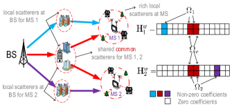
Figure 2: Illustration of joint channel sparsity structure due to the limited and shared local scattering effect at the BS side. $\Omega_{c}$ is the support of the common scatterers shared by all users, while $\Omega_{i}$ is the support of the individual scatterers for the $i$-th user.

We assume a uniform linear array (ULA) model for the antennas installed at the BS and the users. Using the virtual angular domain representation [26], the channel matrix $\mathbf{H}_{i}$ can be expressed as

$$\mathbf{H}_{i}=\mathbf{A}_{R}\mathbf{H}_{i}^{w}\mathbf{A}_{T}^{H},$$

where $\mathbf{A}_{R}\in\mathbb{C}^{N\times N}$ and $\mathbf{A}_{T}\in\mathbb{C}^{M\times M}$ denote the unitary matrices for the angular domain transformation at the user side and BS respectively, $\mathbf{H}_{i}^{w}\in\mathbb{C}^{N\times M}$ is the angular domain channel matrix, where its $(p,q)$-th entry being non-zero indicates that there is a spatial path from the the $q$-th transmit direction of the BS to the $p$-th receive direction of the $i$-th user (see detailed physical explanation of this model in [26]). In multi-user massive MIMO systems, as indicated by experimental study [12], the angular domain channel matrices $\{\mathbf{H}_{i}^{w}\}$ are in general sparse due to the limited local scattering effects at the BS side. Denote the $j$-th row of $\mathbf{H}_{i}^{w}$ as $\mathbf{h}_{ij}$. Denote $\textrm{supp}(\mathbf{h})$ as the index set of the non-zero entries of vector $\mathbf{h}$, i.e., $\textrm{supp}(\mathbf{h})=\{i:\mathbf{h}(i)\neq 0\}$. Based on many practical measurements of the channel matrices of massive MIMO systems [14, 13, 15, 16], we have the following two important observations:

• Observation I (Sparsity Support within Individual Channel Matrix): From [14, 13], the massive MIMO channels are usually correlated at the BS side but not at the user side. This is due to the limited scattering at the BS side, and relatively rich scattering at the users (as illustrated in Figure 2). Hence, the row vectors within an $\mathbf{H}_{i}^{w}$ usually have the same sparsity support, i.e., $\textrm{supp}(\mathbf{h}_{i1})=\textrm{supp}(\mathbf{h}_{i2})=\cdots\textrm{supp}(\mathbf{h}_{iN})$. Notice that in practical multi-user massive MIMO downlinks, the BS is usually elevated very high, with limited scatterers (relative to the number of antennas). Hence, the BS might only have a few active transmit directions for each user. However, the mobile users are usually at low elevation, such that the users have relatively rich local scatterers isotropically.

• Observation II (Partially Shared Support between Different Channel Matrices): From [14, 15, 16], the channel matrices of different users are usually correlated (inter-channel correlation), especially when the users are physically close to each other. From these results [14, 15, 16], different users tend to share some common local scatterers at the BS [19] (as illustrated in Figure 2) and hence, their channel matrices $\{\mathbf{H}_{i}^{w}\}$ may have a partially common support. Specifically, there may exist a non-zero index set $\Omega_{c}$ of the common support, such that $\Omega_{c}\subseteq\Omega_{i}$, for all $i$.

Note that Observation I refers to the individual joint sparsity within each channel matrix, while Observation II refers to the distributed joint sparsity among the user channel matrices. In the special case when each user has $N=1$ antenna, each $\mathbf{H}_{i}^{w}$ would be reduced to a row vector and hence the individual joint sparsity from Observation I vanishes. Based on the above Observations, we have the following assumption on the channel matrices in multi-user massive MIMO systems.

Definition 1 (Joint Sparse Massive MIMO Channel)

The channel matrices $\{\mathbf{H}_{i}^{w}:\forall i\}$ have the following properties:

(a) Individual joint sparsity due to local scattering at the BS: Denote $\mathbf{h}_{ij}$ as the $j$-th row vector of $\mathbf{H}_{i}^{w}$; then $\{\mathbf{h}_{ij}:\forall j\}$ are simultaneously sparse, i.e., there exists an index set $\Omega_{i}$, $0<|\Omega_{i}|\ll M$, $\forall i$, such that

$$\textrm{supp}(\mathbf{h}_{i1})=\textrm{supp}(\mathbf{h}_{i2})=\cdots\textrm{supp}(\mathbf{h}_{iN})\triangleq\Omega_{i}.$$ (4)

(b) Distributed joint sparsity due to common scattering at the BS: Different $\{\mathbf{H}_{i}^{w}:\forall i\}$ share a common support, i.e., there exists an index set $\Omega_{c}$ such that

$$\bigcap_{i=1}^{K}\Omega_{i}=\Omega_{c}.$$ (5)

Furthermore, the entries of $(\mathbf{H}_{i}^{w})_{\Omega_{i}}$ are i.i.d. complex Gaussian distributed with zero mean and unit variance, where $(\mathbf{H}_{i}^{w})_{\Omega_{i}}$ denotes the sub matrix formed by collecting the column vectors of $\mathbf{H}_{i}^{w}$ whose indices belong to $\Omega_{i}$. ∎

From Definition 1, the massive MIMO channel sparsity support is parametrized by $\mathcal{P}=\{\Omega_{c},\{\Omega_{i}:\forall i\}\}$, where $\Omega_{i}$ determines the individual sparsity support and $\Omega_{c}$ determines the shared common sparsity support. When $\Omega_{c}=\Omega_{i}$, $\forall i$, this reduces to the scenario in which all users share the same local scatterers at the BS side, and when $\Omega_{c}=\emptyset$, this reduces to the scenario in which no common scatterers are shared by the users. We assume there is a statistical bound on the channel sparsity levels ($\left|\Omega_{c}\right|$, $|\Omega_{i}|$), i.e. $\Pr\left(\Lambda\right)>1-\varepsilon$ for some small $\varepsilon$, where event $\Lambda$ denotes

$$\Lambda:\quad\left|\Omega_{c}\right|\geq s_{c},\;|\Omega_{i}|\leq s_{i},\forall i.$$ (6)

and $\mathbb{S}=\left\{s_{c},\{s_{i}:\forall i\}\right\}$ ($s_{c}$, $s_{i}\ll M$) refers to the statistical sparsity bounds. Note that the BS and the MSs have no knowledge of the random channel support realizations $\mathcal{P}$. However, we assume the statistical sparsity bound $\mathbb{S}=\left\{s_{c},\{s_{i}:\forall i\}\right\}$ is available to the BS. In practice, the channel sparsity statistics $\mathbb{S}$ depends on the large scale properties of the scattering environment and changes slowly (over a very long timescale). Hence, knowledge of $\mathbb{S}$ can be obtained easily based on the prior knowledge of the propagation environment (e.g., can be acquired from offline channel propagation measurement at the BS as in [20] or long term stochastic learning and estimation [27]). Based on the above channel model, we shall elaborate our distributed CSIT estimation and feedback framework in the next section.

II-C Distributed Compressive CSIT Estimation and Feedback

In order to overcome the issue of pilot training and feedback overhead in multi-user massive MIMO, we shall exploit the joint channel sparsity structure defined in Definition 1. Specifically, instead of recovering each $\mathbf{H}_{i}$ based on the observed output symbols $\mathbf{Y}_{i}$ individually at the $i$-th user [28, 18, 17], we shall propose a novel CSIT estimation and feedback framework in which the compressed measurements $\{\mathbf{Y}_{i}\}$ are observed distributively at the users, while the $\{\mathbf{H}_{i}\}$ is recovered jointly at the BS. This novel estimation topology allows us to exploit the distributed joint sparsity among the user channel matrices to reduce the estimation and feedback overhead to maintain a target CSIT estimation quality. The distributed CSIT estimation and feedback algorithm is described in the following and is also illustrated in Figure 3.

Algorithm 1 (Distributed Compressive CSIT Estimation and Feedback)

• Step 1 (Pilot Training): The BS sends the compressive training symbols $\mathbf{X}\in\mathbb{C}^{M\times T}$, with $T\ll M$.

• Step 2 (Compressive Measurement and Feedback): The $i$-th mobile user observes the compressed measurements $\mathbf{Y}_{i}$ from the pilot symbols given in (2) and feeds back to the BS side.

• Step 3 (Joint CSIT Recovery at BS): The BS recovers the CSIT $\{\mathbf{H}_{1}^{e},\cdots,\mathbf{H}_{K}^{e}\}$ jointly based on the compressed feedback $\{\mathbf{Y}_{1},\cdots,\mathbf{Y}_{K}\}$. ∎

Obviously, the pilot training and feedback overhead in Algorithm 1 are characterized by $T$. Our goal is to exploit the hidden joint channel sparsity in the CSIT recovery in Step 3 of Algorithm 1 to reduce the required training and feedback overhead $T$ in multi-user massive MIMO systems. The problem of CSIT recovery at the BS (Step 3) can be formulated as follows:

Problem 1 (Joint CSIT Recovery at BS)

$$\min_{\{\mathbf{H}_{i},\forall i\}} \sum_{i=1}^{K}\left\|\mathbf{Y}_{i}-\mathbf{H}_{i}\mathbf{X}\right\|_{F}^{2}$$

s.t. $$\left\{\mathbf{H}_{i}^{w}:\forall i\right\}\mbox{ satisfy the joint sparsity}$$ (7)

model as in Definition 1.

∎

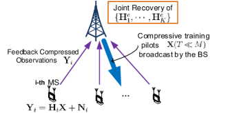
Figure 3: The BS broadcasts compressive training pilot $\mathbf{X}\in\mathbb{C}^{M\times T}$ (with $T\ll M$) to all the $K$ mobile users. Each user locally obtains the compressive measurement $\mathbf{Y}_{i}$ and feeds back to the BS. The BS jointly recovers the CSIT $\{\mathbf{H}_{1}^{e},\cdots,\mathbf{H}_{K}^{e}\}$ based on the obtained compressive measurements $\{\mathbf{Y}_{1},\cdots,\mathbf{Y}_{K}\}$.

However, Problem 1 is very challenging due to the individual and distributed joint sparsity requirement in constraint (7). This is quite different from the conventional CS-recovery problem with a simple sparsity ($\mbox{l}_{0}$-norm) constraint. In later sections, we shall propose a low complexity greedy algorithm to solve Problem 1.

Challenge 1: Design a low complexity algorithm to solve Problem 1 despite challenging constraint (7).

III Joint CSIT Recovery Algorithm Design

In this section, we shall propose a low complexity algorithm to solve Problem 1 by exploiting the hidden sparsity structures of the channel matrices (Definition 1). To achieve this, we first rewrite (2) into the standard CS model. Denote the following new variables:

$$\mathbf{\bar{Y}}_{i}=\sqrt{\frac{M}{PT}}\mathbf{Y}_{i}^{H}\mathbf{A}_{R}\in\mathbb{C}^{T\times N},\;\bar{\mathbf{X}}=\sqrt{\frac{M}{PT}}\mathbf{X}^{H}\mathbf{A}_{T}\in\mathbb{C}^{T\times M},$$ (8)

$$\mathbf{\bar{H}}_{i}=(\mathbf{H}_{i}^{w})^{H}\in\mathbb{C}^{M\times N},\;\mathbf{\bar{N}}_{i}=\sqrt{\frac{M}{PT}}\mathbf{N}_{i}^{H}\mathbf{A}_{R}\in\mathbb{C}^{T\times N}.$$ (9)

Substituting these variables into (2), we obtain

$$\mathbf{\bar{Y}}_{i}=\bar{\mathbf{X}}\mathbf{\bar{H}}_{i}+\mathbf{\bar{N}}_{i},\forall i.$$ (10)

Then (10) matches the standard CS measurement model, where $\bar{\mathbf{X}}$ is the measurement matrix with $\textrm{tr}(\bar{\mathbf{X}}^{H}\bar{\mathbf{X}})=M$ and $\mathbf{\bar{H}}_{i}$ is the sparse matrix. Further note that

$$\left\|\mathbf{\bar{Y}}_{i}-\bar{\mathbf{X}}\mathbf{\bar{H}}_{i}\right\|_{F}^{2}=\frac{M}{PT}\left\|\mathbf{Y}_{i}-\mathbf{H}_{i}\mathbf{X}\right\|_{F}^{2},\forall i$$

and hence solving Problem 1 is equivalent to finding $\{\mathbf{\bar{H}}_{i}:\forall i\}$ to minimize $(\sum_{i=1}^{K}\left\|\mathbf{\bar{Y}}_{i}-\bar{\mathbf{X}}\mathbf{\bar{H}}_{i}\right\|_{F}^{2})$ subject to the joint sparsity constraint (7). Based on this equivalence relationship and equation (10), we elaborate our designed algorithm to solve Problem 1 in the following.

III-A Proposed J-OMP Algorithm

In the literature, numerous algorithms [29, 30, 31, 32, 33, 34, 35, 36, 37, 38] have been proposed to solve the CS problems either with or without structured sparsity of the signal sources. Classical CS recovery algorithms that consider general sparse signals without structured sparsity include the basis pursuit (BP) [29], orthogonal matching pursuit (OMP) [30], and many variants of OMP such as the compressive sampling matching pursuit (CoSaMP) [31] and subspace pursuit (SP) [32]. Based on these initial CS works [29, 30, 31, 32], many later works [33, 34, 36, 35, 37, 38] have considered structured sparse signals and looked for approaches to exploit the structured sparsity properties. For instance, in [33, 34], a simultaneous OMP (SOMP) algorithm is proposed to solve the multiple measurement vector (MMV) problems [33]. In [35, 36], a mixed-norm BP is developed to recover the block sparse signals and in [37], a select-discard OMP (SD-OMP) is proposed to recover partially joint sparse signals. However, these joint sparsity structures [33, 34, 36, 37, 35] do not cover the cases of the channel matrices $\{\mathbf{H}_{i}^{w}\}$ in this paper and hence, the associated algorithms [33, 34, 36, 37, 35] is not suitable to solve our problem (Problem 1). In [38], a model-based CS framework is further proposed to model the structured sparse signals and some sparse approximation algorithms are proposed to recover several special classses of structured sparse signals. However, this framework cannot be extended to our problem because the pruning step in the model-based CoSaMP[38] is still combinatorial under our scenario. In this section, we shall propose a novel joint orthogonal matching pursuit (J-OMP) algorithm to solve Problem 1. Specifically, the proposed J-OMP algorithm is designed by extending conventional OMP [30] to adapt to the specific sparsity structures of massive MIMO channels discussed in Section II.

Denote $\mathbf{A}^{\Omega}$ as the sub matrix formed by collecting the row vectors of $\mathbf{A}$ whose indices belong to $\Omega$. The details of the proposed algorithm are given below:

Algorithm 2 (Joint-OMP to Solve Problem 1)

Input: $\{\mathbf{Y}_{i}:\forall i\}$, $\mathbf{X}$, $\mathbb{S}=\left\{s_{c},\{s_{i}:\forall i\}\right\}$, $\eta_{1}$, $\eta_{2}$ $(\eta_{1}<1,\eta_{2}>1)$.

Output: Estimated $\{\mathbf{\mathbf{H}}_{i}^{e}\}$ for $\{\mathbf{\mathbf{H}}_{i}:\forall i\}$.

• Step 1 (Initialization): Compute $\mathbf{\bar{Y}}_{i}$, $\forall i$, $\bar{\mathbf{X}}$ from $\{\mathbf{Y}_{i}:\forall i\}$ and $\mathbf{X}$, as in (8).

• Step 2 (Common Support Identification): Initialize $\mathbf{R}_{i}=\mathbf{\bar{Y}}_{i}$, $\forall i$, $\Omega_{c}^{e}=\emptyset$ and then repeat the following procedures $s_{c}$ times.

  • A (Support Estimate): Estimate the remaining index set by $\Omega_{i}^{{}^{\prime}}=\arg\max_{\left|\Omega\right|=s_{i}-|\Omega_{c}^{e}|}\left\|(\bar{\mathbf{X}}_{\Omega})^{H}\mathbf{R}_{i}\right\|_{F}$, $\forall i$.

  • B (Support Pruning): Prune support $\Omega_{i}^{{}^{\prime}}$ to be $\Omega_{i}^{{}^{\prime}}=\left\{j:\,j\in\Omega_{i}^{{}^{\prime}},\left\|\bar{\mathbf{X}}(j)^{H}\mathbf{R}_{i}\right\|_{F}^{2}\geq\eta_{1}N\right\}$, $\forall i$.

  • C (Support Update): Update the estimated common support as $\Omega_{c}^{e}=\Omega_{c}^{e}\bigcup\left\{\textrm{arg}\max_{j}\sum_{i=1}^{K}I_{\{j\in\Omega_{i}^{{}^{\prime}}\}}\right\}.$

  • D (Residual Update): $\mathbf{R}_{i}=\left(\mathbf{I}-\mathbf{P}_{\Omega_{c}^{e}}\right)\mathbf{\bar{Y}}_{i}$, where $\mathbf{P}_{\Omega_{c}}$ is a projection matrix and is given by

    $$\mathbf{P}_{\Omega_{c}^{e}}=(\bar{\mathbf{X}}_{\Omega_{c}^{e}})(\bar{\mathbf{X}}_{\Omega_{c}^{e}})^{\dagger}.$$ (11)

• Step 3 (Individual Support Identification): Set $\Omega_{i}^{e}=\Omega_{c}^{e}$, $\forall i$ and estimate the individual support $\Omega_{i}^{e}$ for each user $i$ individually. Specifically, for the $i$-th user, stop if $||\mathbf{R}_{i}||_{F}^{2}\leq\frac{\eta_{2}NM}{P}$ or the following procedures have been repeated $(s_{i}-s_{c})$ times.

  • A (Support Update): Update the estimated individual support as $\Omega_{i}^{e}=\Omega_{i}^{e}\bigcup\left\{\arg\max_{j}\left\|\bar{\mathbf{X}}(j)^{H}\mathbf{R}_{i}\right\|_{F}\right\}$.

  • B (Residual Update): $\mathbf{R}_{i}=\left(\mathbf{I}-\mathbf{P}_{\Omega_{i}^{e}}\right)\mathbf{\bar{Y}}_{i}$.

• Step 4 (Channel Estimation by LS): The estimated channel for user $i$ is $\mathbf{\mathbf{H}}_{i}^{e}=\mathbf{A}_{R}(\mathbf{\mathbf{\bar{H}}}_{i}^{e})^{H}\mathbf{A}_{T}^{H}$, where $\mathbf{\mathbf{\bar{H}}}_{i}^{e}$ is given by $\left(\mathbf{\mathbf{\bar{H}}}_{i}^{e}\right)^{\Omega_{i}^{e}}=\left(\bar{\mathbf{X}}_{\Omega_{i}^{e}}\right)^{\dagger}\mathbf{\bar{Y}}_{i}$, $\left(\mathbf{\mathbf{\bar{H}}}_{i}^{e}\right)^{[M]\backslash\Omega_{i}^{e}}=\mathbf{0}$, $\forall i$. ∎

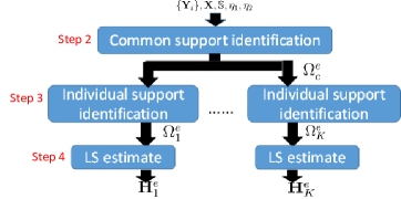
Figure 4: Main processing flow of Algorithm 2.

Note that $\eta_{1}$, $\eta_{2}$ ($\eta_{1}<1$, $\eta_{2}>1$) in the input of Algorithm 2 are threshold parameters (as in Step 2 B and Step 3). In Algorithm 2, Step 2 and 3 aim to identify the common support $\Omega_{c}$ and the individual support $\Omega_{i}$ respectively. Based on the estimated individual support $\Omega_{i}^{e}$, Step 4 recovers the channel matrices using the LS approach, as illustrated in Figure 4. In Algorithm 2, the following two strategies have been utilized to exploit the individual and distributed joint sparsity in the user channel matrices.

• Strategy to exploit Observation I: Note that the estimation target $\mathbf{\bar{H}}_{i}$ in (10) is simultaneously zero or non-zero on each row of $N$ entries. Hence, similar to the simultaneous recovery algorithm proposed for MMV problems [34], we consider identifying a row vector of $\mathbf{\bar{H}}_{i}$ an atomic unit, based on the aggregate matching effects between the residual $\mathbf{R}_{i}$ and the measurement matrix $\bar{\mathbf{X}}$. For instance, we select the support index based on the sum of the $N$ matched terms corresponding to the $N$ columns of the residual matrix $\mathbf{R}_{i}$, i.e., $\sqrt{\sum_{l=1}^{N}||\bar{\mathbf{X}}(j)^{H}\mathbf{R}_{i}(l)||^{2}}=||\bar{\mathbf{X}}(j)^{H}\mathbf{R}_{i}||_{F}$, as in Step 2. A and Step 3. A.

• Strategy to exploit Observation II: Note that $\{\mathbf{\bar{H}}_{i}\}$ share a partial common support $\Omega_{c}$. This indicates that the indices in $\Omega_{c}$ are very likely to be estimated by most of the users. For instance, if $\Omega_{c}=\{i_{1}\}$, then index $i_{1}$ is likely to be estimated as the support index by each of the $K$ users. Reversely speaking, the index identified by the largest number of users is very likely to be $i_{1}$. Based on this intuition, we have designed a joint selection process among different users in Step 2. B, and we identify the index that appears the largest number of times in the estimated support $\Omega_{i}^{{}^{\prime}}$, $\forall i$, as the next identified common support index (as in Step 2. B).

Remark 1 (Characterization of Algorithm 2)

Suppose $s_{i}=s$, $\forall i$, for simplicity. The overall complexity of Algorithm 2 is $O(KsMNT)$, which is the same order as recovering each $\mathbf{\mathbf{\bar{H}}}_{i}$ individually using the conventional 2-norm SOMP[34, 39]. Furthermore, compared with some conventional CS recovery algorithm (e.g. OMP in [30]) or sparse channel estimation [20] in which knowledge of instantaneous sparsity level is needed, the proposed J-OMP requires only the statistical channel sparsity information $\mathbb{S}$, which can be estimated using slow-timescale stochastic learning [27].

III-B Analysis of Support Recovery Probability for the Proposed J-OMP Algorithm

First of all, suppose $s_{i}$ in $\mathbb{S}$ are the same, i.e, $s_{i}=s$, $\forall i$, to obtain simple expressions. In classical CS works [31, 32], the restricted isometry property (RIP) is used to characterize the measurement matrix to facilitate the performance analysis of CS recovery algorithms. We first review the notion of the RIP in the following:

Definition 2 (Restricted Isometry Property [32])

Matrix $\bar{\mathbf{X}}\in\mathbb{C}^{T\times M}$ satisfies the RIP of order $k$ with the restricted isometry constant (RIC) $\delta_{k}$ if $0\leq\delta_{k}<1$ and $\delta_{k}$ is the smallest number such that

$$(1-\delta_{k})\left\|\mathbf{h}\right\|^{2}\leq\left\|\bar{\mathbf{X}}\mathbf{h}\right\|^{2}\leq(1+\delta_{k})\left\|\mathbf{h}\right\|^{2}$$

holds for all $\mathbf{h}\in\mathbb{C}^{M\times 1}$ where $\left\|\mathbf{h}\right\|_{0}\leq k$. ∎

In the following analysis, we assume that the measurement matrix $\bar{\mathbf{X}}$ satisfies the RIP property and the specific requirements on the RICs (e.g. $\delta_{s}$, $\delta_{2s}$, etc.) will be given in each theorem. Specifically, we are interested in the following support recovery events $\Theta_{c}$, $\{\Theta_{i}\}$ in Algorithm 2:

$$\Theta_{c}:\textrm{ in Step 2 of Alg. 2, support }$$

$$\Omega_{c}^{e}\; \Omega_{c}^{e}\subseteq\Omega_{c}$$is correctly identified, i.e., . (12)

$$\Theta_{i}:\textrm{ in Step 3 of Alg. 2, support $\Omega_{i}^{e}$}$$

is correctly identified, i.e., $$\Omega_{i}^{e}=\Omega_{i}$$. (13)

We shall analyze the probability of these support recovery events (i.e., $\Theta_{c}$, $\{\Theta_{i}\}$) because they are closely related to the final CSIT estimation quality and the higher the support recovery probabilities, the better the CSIT estimation quality should be. (We formally discuss this in Theorem 3 in Section IV.) Denote $[M]=\{1,2,\cdots,M\}$ and suppose there is a $K_{0}$ such that

$$\max_{j\in[M]\backslash\Omega_{c}}\sum_{i=1}^{K}I_{\{j\in\Omega_{i}\}}\leq K_{o}$$ (14)

where $K_{o}<K$ from (5). Denote $\gamma\triangleq\frac{K_{o}}{K}<1$. Based on these preparations, we analyze the probabilities of the support recovery events (i.e., $\Theta_{c}$, $\{\Theta_{i}\}$) by averaging the support recovery outcomes with respect to (w.r.t.) the randomness of the channel matrices (Definition 1). We first have the following probability bound of event $\Theta_{c}$ conditioned on $\Lambda$ (given in (6)).

Theorem 1 (Probability Bounds of $\Theta_{c}\mid\Lambda$)

If $\theta$ and $p$ in the following satisfy

$$\theta \triangleq \min\left(\frac{\left(1-2\delta_{s}\right)}{\left(\delta_{s+1}+2(1-\delta_{s})\sqrt{\frac{(1+\delta_{1})\eta_{2}M}{P}}\right)},\right.$$

$$\frac{\left(1-2\delta_{s}\right)^{2}}{(1-\delta_{s})^{2}\left(\sqrt{\eta_{1}}+\sqrt{\frac{(1+\delta_{1})\eta_{2}M}{P}}\right)^{2}},$$

$$\left.\frac{\left(\sqrt{\eta_{1}}-\sqrt{\frac{\eta_{2}M(1+\delta_{1})}{P}}\right)^{2}(1-\delta_{s})^{2}}{\delta_{s+1}^{2}}\right)>1,$$

$$p\triangleq 2\cdot\exp\left(-N\left(\ln\theta-1+\frac{1}{\theta}\right)\right)+M\cdot\exp\left(-N\times\right.$$

$$\left.\left(\theta-1-\ln\theta\right)\right)+\exp\left(-NT\left(\eta_{2}-\ln\eta_{2}-1\right)\right)<1,$$ (16)

then the conditional probability of event $\Theta_{c}$ given $\Lambda$, denoted as $\textrm{Pr}(\Theta_{c}\mid\Lambda)$, satisfies

$$\textrm{Pr}(\Theta_{c}\mid\Lambda)\geq 1-2c_{0}\sum_{t=0}^{\left\lceil\frac{1+\gamma}{2}K\right\rceil}\left(\begin{array}[]{c}K\\ t\end{array}\right)(1-p)^{t}p^{K-t},$$ (17)

where $\eta_{1}<1,$ $\eta_{2}>1$ are the threshold parameters in Algorithm 2, $c_{0}=\sum_{t=0}^{s_{c}}\left(\begin{array}[]{c}s\\ t\end{array}\right)-1$, $\delta_{1}$, $\delta_{s}$ and $\delta_{s+1}$ are the $1$-th, $s$-th and $(s+1)$-th RIC respectively of $\bar{\mathbf{X}}$.

Proof:

See Appendix -A. ∎

We also have the following results regarding the conditional event of $\Theta_{i}$ given $\Theta_{c}$ and $\Lambda$, (denoted as $\Theta_{i}\mid\Theta_{c}\Lambda$), $\forall i$.

Theorem 2 (Probability Bounds of $\Theta_{i}\mid\Theta_{c}\Lambda$)

Denote $\vartheta\triangleq\frac{(1-\delta_{s})P}{4\eta_{2}M}$. If (1) holds, then the conditional probability of event $\Theta_{i}$ given $\Theta_{c}$ and $\Lambda$, denoted as $\textrm{Pr}(\Theta_{i}\mid\Theta_{c}\Lambda)$, satisfies

$$\textrm{Pr}\left(\Theta_{i}\mid\Theta_{c}\Lambda\right)\geq 1-c_{i}\cdot\exp\left(-N\left(\ln\theta-1+\frac{1}{\theta}\right)\right)-$$

$$c_{i}M\cdot\exp\left(-N\left(\theta-1-\ln\theta\right)\right)-s\cdot\exp\left(-N\vphantom{\left(\ln\vartheta-1+\frac{1}{\vartheta}\right)}\right.$$ (18)

$$\left.\times\left(\ln\vartheta-1+\frac{1}{\vartheta}\right)\right)-\exp\left(-NT\left(\eta_{2}-\ln\eta_{2}-1\right)\right),$$

where $c_{i}=\sum_{t=s_{c}}^{s}\left(\begin{array}[]{c}s\\ t\end{array}\right)-1$.

Proof:

Please see Appendix -C. ∎

Note that Theorem 1 and 2 bound the support recovery probabilities in terms of the joint channel sparsity parameters ($N$, $K$, $\Omega_{c}$, etc.). On the other hand, intuitively, the channel support recovery probability is also closely related to the final CSIT estimation quality. As such, Theorem 1 and 2 may allow us to obtain simple insights regarding how the joint channel sparsity can benefit the CSIT estimation performance. We will have detailed discussions of this in Section IV.

III-C Discussion of the Pilot Training Matrix $\mathbf{X}$

Under the proposed CSIT estimation scheme, one issue that remains to be discussed is how to design the entries of the $M\times T$ pilot training matrix $\mathbf{X}$. In the CS literature, the RIP property [29] is widely used to characterize the quality of a CS measurement matrix. It is shown that efficient and robust CS recovery can be achieved when the measurement matrix satisfies a proper RIC $\delta_{s}$ requirement (see Definition 2). On the other hand, CS measurement matrices randomly generated from the sub-Gaussian distribution [39] can satisfy the RIP property with overwhelming probability [39]. As such, this generation approach for the CS measurement matrix is also widely used [18, 17]. Among the sub-Gaussian family, the Rademacher distribution is commonly adopted due to its simplicity, and it is also frequently utilized to generate the pilot training matrix in conventional CS-based channel estimation designs [18, 17]. Based on this and from the signal model in (2), the pilot training matrix $\mathbf{X}\in\mathbb{C}^{M\times T}$ can be designed as $\mathbf{X}=\mathbf{A}_{T}\mathbf{X}_{a}$, where $\mathbf{X}_{a}\in\mathbb{C}^{M\times T}$ is i.i.d. drawn from $\left\{-\sqrt{\frac{P}{M}},\sqrt{\frac{P}{M}}\right\}$, with equal probability.

IV CSIT Estimation Quality in Multi-user Massive MIMO Systems

In this section, we analyze the CSIT estimation performance in terms of the normalized mean absolute error [40] of the channel matrices. From the closed-form results, we can obtain simple insights into how the joint sparsity of the user channel matrices can be exploited to enhance the CSIT estimation performance.

Challenge 2: Derive closed-form tradeoff analysis to obtain insights into how the joint channel sparsity can be utilized to enhance the CSIT estimation performance.

IV-A Estimation Error of the CSIT in Multi-user Massive MIMO

By analyzing the CSI distortion under both correct and incorrect channel support recoveries, we obtain the following theorem on the normalized mean absolute error (NMAE) [40] of the channel matrices. Note that we still assume $s_{i}=s$, $\forall i$, in the statistical information $\mathbb{S}$ to obtain simple expressions.

Theorem 3 (CSIT Estimation Quality)

The normalized mean absolute error (NMAE) [40] of $\mathbf{H}_{i}$ satisfies

$$\mathbb{E}\left(\frac{\left\|\mathbf{H}_{i}-\mathbf{H}_{i}^{e}\right\|_{F}}{\left\|\mathbf{H}_{i}\right\|_{F}}\right) \leq \sqrt{\frac{MNs}{PT(1-\delta_{s})}}\frac{\Gamma\left(N-\frac{1}{2}\right)}{\Gamma\left(N\right)}+$$

$$C_{i}+E_{i}+\varepsilon\left(1+\sqrt{\frac{1+\delta_{1}}{1-\delta_{s}}}\right)$$

where $\Gamma(\cdot)$ is the gamma function and

$$C_{i}=\left(1-\textrm{Pr}(\Theta_{c}\mid\Lambda)\right)\left(\frac{1-\delta_{s}+\delta_{2s}}{1-\delta_{s}}\right),$$

$$E_{i}=\left(1-\textrm{Pr}\left(\Theta_{i}\mid\Theta_{c}\Lambda\right)\right)\left(\frac{1-\delta_{s}+\delta_{2s}}{1-\delta_{s}}\right).$$

where $\textrm{Pr}(\Theta_{c}\mid\Lambda)$ and $\textrm{Pr}\left(\Theta_{i}\mid\Theta_{c}\Lambda\right)$ are the probabilities of the conditional events $\Theta_{c}\mid\Lambda$ and $\Theta_{i}\mid\Theta_{c}\Lambda$ respectively, and $\delta_{1}$, $\delta_{s}$ and $\delta_{2s}$ are the 1-th, $s$-th and $2s$-th RIC of $\bar{\mathbf{X}}$ respectively.

Proof:

See Appendix -D. ∎

Note that the term $\varepsilon\left(1+\sqrt{\frac{1+\delta_{1}}{1-\delta_{s}}}\right)$ in (3) comes from statistical sparsity model in (6), and the terms $C_{i}$ and $E_{i}$ in (3) come from the recovery distortion in Step 2 (common support recovery) and Step 3 (individual support recovery) of Algorithm 2 respectively. From (3), a larger support recovery probabilities of $\textrm{Pr}(\Theta_{c}\mid\Lambda)$ and $\textrm{Pr}\left(\Theta_{i}\mid\Theta_{c}\Lambda\right)$ lead to a smaller $C_{i}$ and $E_{i}$ and hence, tend to have smaller CSIT distortion. As such, Theorem 3 connects the support recovery probability results in Theorem 1 and 2 with the final CSIT estimation quality. Based on Theorem 1, 2 and 3, we discuss how the CSIT estimation quality is affected by the joint channel sparsity in the next section.

IV-B CSIT Estimation Quality w.r.t. Joint Channel Sparsity

Recall that in Section II, we observe (i) that the channel matrix $\mathbf{H}_{i}^{w}$ is simultaneously zero or non-zero on its columns, with dimension $N\times 1$, and (ii) that the $K$ users share a partial common channel support $\Omega_{c}$. Therefore, it is interesting to see how the CSIT estimation quality is affected by these joint sparsity parameters ($N$, $K$, $\Omega_{c}$). Based on Theorem 1, 2 and 3, we obtain the following results (Corollary 1-3).

Corollary 1 (CSIT Quality w.r.t. $N$)

If $\theta$ and $p$, given in (1), (16), satisfy $\theta>1$ and $p<1$, then

$$\lim_{N\rightarrow\infty}-\frac{1}{N}\ln\left(C_{i}\right)\geq\left\lfloor\frac{1-\gamma}{2}K\right\rfloor\beta_{1},$$ (20)

$$\lim_{N\rightarrow\infty}-\frac{1}{N}\ln\left(E_{i}\right)\geq\beta_{2},\quad\forall i,$$ (21)

where $\beta_{1}\triangleq\min\left(\ln\theta-1+\frac{1}{\theta},\,\theta-1-\ln\theta,\,T\left(\eta_{2}-\ln\eta_{2}\right.\right.$ $\left.\left.-1\vphantom{\eta_{2}-\ln\eta_{2}}\right)\right)>0$, $\beta_{2}\triangleq\min\left(\ln\theta-1+\frac{1}{\theta},\,\theta-1-\ln\theta,\,\ln\vartheta-1\right.,$ $\left.+\frac{1}{\vartheta},\;T\left(\eta_{2}-\ln\eta_{2}-1\right)\vphantom{\ln\vartheta-1+\frac{1}{\vartheta}}\right)>0$.

Proof:

See Appendix -E.∎

Remark 2 (Interpretation of Corollary 1)

Equation (20) and (21) can be re-written as

$$C_{i}\leq\exp\left(-N\left\lfloor\frac{1-\gamma}{2}K\right\rfloor\beta_{1}+o(N)\right),$$ (22)

$$E_{i}\leq\exp\left(-N\cdot\beta_{2}+o(N)\right).$$ (23)

From (22) and (23), we conclude that $C_{i}$ and $E_{i}$ in (3) decay at least exponentially w.r.t. $N$ and hence, a larger $N$ turns out to have a smaller CSIT estimation error from Theorem 3. This result indicates that by simultaneously recovering each column of $\mathbf{H}_{i}^{w}$ as an atomic unit, as in Algorithm 2, we capture the individual joint sparsity structure in the user channel matrices (corresponding to Observation I). As such, a larger number of antennas $N$ at the users turn out to have a better CSIT estimation performance.

Corollary 2 (CSIT Quality w.r.t. $K$)

If (1) holds and $p$ in (16) satisfies $p<\frac{1}{2}(1-\gamma)$, then

$$-\lim_{K\rightarrow\infty}\frac{1}{K}\ln\left(C_{i}\right)\geq R_{K}\triangleq$$ (24)

$$\qquad\frac{1-\gamma}{2}\ln\frac{(1-p)(1-\gamma)}{p(1+\gamma)}-\ln\frac{2(1-p)}{(1+\gamma)}>0.$$

Proof:

Please see Appendix -F. ∎

Remark 3 (Interpretation of Corollary 2)

Equation (24) can be re-written as

$$C_{i}\leq\exp\left(-K\cdot R_{K}+o(K)\right),$$ (25)

where $R_{K}$ is given in (24). From (25), we conclude that upper bound term $C_{i}$ in (3) decays at least exponentially w.r.t. the number of mobile users $K$ sharing the common channel support $\Omega_{c}$. This fact indicates that the distributed joint sparsity among the user channel matrices (corresponding to Observation II) is indeed captured by the proposed recovery algorithm and a larger $K$ tends to have a better CSIT estimation performance.

Corollary 3 (CSIT Quality w.r.t. $\Omega_{c}$)

Suppose $\varepsilon=0$ in (6). Scale the threshold parameter $\eta_{2}$ in Algorithm 2 as $\eta_{2}=\sqrt{P}$ and let the transmit SNR $P\rightarrow\infty$, the number of users $K\rightarrow\infty$. If (1) holds and $p$ in (16) satisfies $p<\frac{1}{2}(1-\gamma)$, we have

$$\mathbb{E}\left(\frac{\left\|\mathbf{H}_{i}-\mathbf{H}_{i}^{e}\right\|_{F}}{\left\|\mathbf{H}_{i}\right\|_{F}}\right)\leq\left(\sum_{t=s_{c}}^{s}\left(\begin{array}[]{c}s\\ t\end{array}\right)-1\right)E,$$ (26)

where $E=\left(\frac{1-\delta_{s}+\delta_{2s}}{1-\delta_{s}}\right)\times\left(\exp\left(-N\left(\ln\theta-1+\frac{1}{\theta}\right)\right)+\right.$ $\left.M\cdot\exp\left(-N\left(\theta-1-\ln\theta\right)\right)\right)$.

Proof:

(Sketch) When (1) holds and $p$ in (16) satisfies $p<\frac{1}{2}(1-\gamma)$, we obtain $\textrm{Pr}(\Theta_{c})\rightarrow 1$ as $K\rightarrow\infty$. From Theorem 3 and Theorem 2, Corollary 3 is obtained. ∎

Remark 4 (Interpretation of Theorem 3)

From (26), $\mathbb{E}\left(\frac{\left\|\mathbf{H}_{i}-\mathbf{H}_{i}^{e}\right\|_{F}}{\left\|\mathbf{H}_{i}\right\|_{F}}\right)\rightarrow 0$ as $s_{c}\rightarrow s$ and hence a larger size (larger $s_{c}$, $s_{c}\leq s$) of the common support $\Omega_{c}$ shared by the users will have a smaller CSIT estimation error. This is because the shared common channel support $\Omega_{c}$ is jointly estimated by the $K$ users (as in Step 2 in Algorithm 2) and hence, is very likely to be recovered when $K\rightarrow\infty$. Therefore, having a larger size of the shared common support $\Omega_{c}$ for the users, will lead to a better CSIT estimation performance in multi-user massive MIMO systems.

Remark 5 (Approximate Performance Comparison)

Consider a baseline (Baseline 3 in Section V) which recovers each channel individually using the 2-norm SOMP [34, 39] (without exploiting the common support). Then this baseline corresponds to using $s_{c}=0$ in Algorithm 2, and the associated upper bound on the CSIT NMAE is given by Corollary 3 (with $s_{c}=0$). Therefore, when $K\rightarrow\infty$ and $s_{c}>\frac{1}{2}s$, the high SNR NMAE ratio of the proposed scheme vs this baseline is given by $\mathcal{O}\left(2^{s\left(\mathcal{H}(\frac{s_{c}}{s})-1\right)}\right)$ ([41] Lemma 16.19), where $\mathcal{H}(\frac{s_{c}}{s})=-\frac{s_{c}}{s}\log\left(\frac{s_{c}}{s}\right)-(1-\frac{s_{c}}{s})\log\left(1-\frac{s_{c}}{s}\right)<1$, $\frac{1}{2}<\frac{s_{c}}{s}\leq 1$. Hence, the NMAE ratio decreases as $s_{c}$ increases (i.e., as $s_{c}\rightarrow s$, $\mathcal{H}(\frac{s_{c}}{s})\rightarrow 0$), which indicates that a larger performance gain of the proposed scheme over this baseline can be achieved as the size of the common support increases (verified in Figure 7 in Section V).

V Numerical Results

In this section, we verify the performance advantages of our proposed CSIT estimation scheme via simulation. Specifically, we compare the proposed J-OMP recovery algorithm with the following state-of-the-art baselines:

• Baseline 1 (Conventional LS): Each $\mathbf{H}_{i}$ is recovered using the conventional LS approach [10, 11], as in (3).

• Baseline 2 (OMP): Each $\mathbf{H}_{i}$ is recovered individually using conventional OMP, which corresponds to a naive extension of CS to CSIT estimations [28, 18, 17].

• Baseline 3 (2-norm SOMP): Each $\mathbf{H}_{i}$ is recovered individually using the 2-norm SOMP [33, 34] to exploit the individual joint channel sparsity.

• Baseline 4 (M-BP): Each $\mathbf{H}_{i}$ is recovered individually using the mixed-norm basis pursuit (M-BP) [35, 36] to exploit the individual joint channel sparsity.

• Baseline 5 (SD-OMP): The $\{\mathbf{H}_{i}\}$ are jointly recovered using the select-discard simultaneous OMP algorithm proposed in [37].

• Baseline 6 (Genie-aided LS): This serves as an performance upper bound scenario, in which we assume the BS knows the channel support $\{\Omega_{i}\}$ with some genie aid and recovers the CSI directly by using $\Omega_{i}$ in Step 4 of Algorithm 2.

We consider a narrow band (flat fading) multi-user massive MIMO FDD system with one BS and $K$ users, where the BS has $M$ antennas and each user has $N$ antennas. Denote the average transmit SNR at the BS as $P$ and the statistical information on the channel sparsity levels as $\mathbb{S}=\{s_{c},\{s_{i}=s:\forall i\}\}$ as in Section II. We use the 3GPP spatial channel model (SCM) [42] to generate the channel coefficients and we assume that the MS has rich local scattering environment as in [43]. On the other hand, the number of individual spatial paths and common spatial paths from the BS broadside (corresponding to the channel sparsity levels $|\Omega_{i}|$, $|\Omega_{c}|$ as in Section II) are randomly generated as $|\Omega_{i}|\sim\mathcal{U}\left(s-2,s\right)$ and $|\Omega_{c}|\sim\mathcal{U}\left(s_{c},s_{c}+2\right)$ respectively (note that $|\Omega_{c}|\geq s_{c}$, $|\Omega_{i}|\leq s$ as in Section II), where $\mathcal{U}(a,b)$ denotes discrete uniform distribution on the integers $\{a,a+1,...,b\}$. The spatial paths from the BS broadside are assumed to have equal path loss and the angle of departures are randomly and uniformly distributed over $[0,2\pi]$. The threshold parameters $\eta_{1}$, $\eta_{2}$ in Algorithm 2 are set to be $\eta_{1}=0.2$, $\eta_{2}=2$.

V-A CSIT Estimation Quality Versus Overhead $T$

In Figure 5, we compare the normalized mean squared error (NMSE) [40] of the estimated CSI versus the training and feedback overhead $T$, under the number of BS antennas $M=160$, number of MS antennas $N=2$, number of users $K=40$, common sparsity parameter $s_{c}=9$, individual sparsity parameter $s=17$ and transmit SNR $P=28$ dB. From this figure, we observe that the CSIT estimation quality increases as $T$ increases and the proposed J-OMP algorithm achieves a substantial performance gain over the baselines. This is because the proposed J-OMP exploits the hidden joint sparsity among the user channel matrices to better recover the CSI. Specifically, the performance gain of the 2-norm SOMP and M-BP schemes over OMP demonstrates the benefits of exploiting the individual joint sparsity within each channel matrix (Observation I), and the performance gain of J-OMP over the 2-norm SOMP and M-BP demonstrates the benefits of exploiting the distributed joint sparsity among the user channel matrices (Observation II). Furthermore, we observe that the proposed J-OMP, 2-norm SOMP, M-BP SD-OMP, and OMP all approach the genie-aided LS scheme as $T$ increases. This is because the channel support recovery probabilities of these schemes all go to 1 as $T$ increases. This fact also highlights the importance of having a higher probability of support recovery in the CSIT reconstruction.

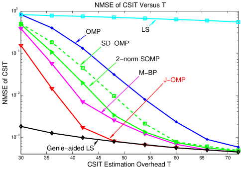
Figure 5: NMSE of CSIT versus the CSIT training and feedback overhead $T$ under $M=160$, $N=2$, $K=40$, $s_{c}=9$, $s=17$ and transmit SNR $P=28$ dB.

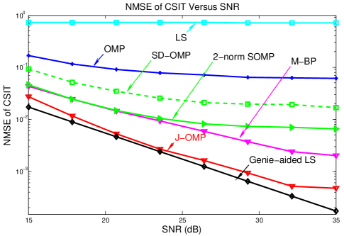
Figure 6: NMSE of CSIT versus the transmit SNR $P$ under under $T=45$, $M=160$, $N=2$, $K=40$, $s_{c}=9$ and $s=17$.

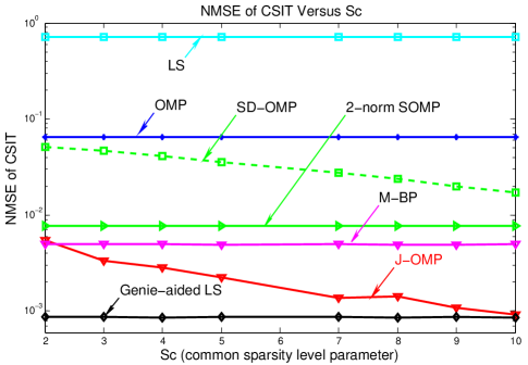
Figure 7: NMSE of CSIT versus the common sparsity $s_{c}$ under $T=45$, $M=160$, $N=2$, $K=40$, $s=17$ and transmit SNR $P=28$ dB.

V-B CSIT Estimation Quality Versus Transmit SNR $P$

In Figure 6, we compare the NMSE of the estimated CSI versus the transmit SNR $P$, under $T=45$, $M=160$, $N=2$, $K=40$, $s_{c}=9$ and $s=17$. From this figure, we observe that the proposed J-OMP algorithm has substantial performance gain over the baselines and relatively larger performance gain is achieved in higher SNR regions.

V-C CSIT Estimation Quality Versus Common Sparsity $s_{c}$

In Figure 7, we compare the NMSE of the estimated CSI versus the common sparsity level parameter $s_{c}$, under $T=45$, $M=160$, $N=2$, $K=40$, $s=17$ and $P=28$ dB. From this figure, we observe that the CSIT estimation quality of the proposed J-OMP scheme gets better as the size of the common support $s_{c}$ increases. This is because the proposed J-OMP scheme exploits the shared common support of the $K$ users and the common support is more likely to be correctly identified as in Algorithm 2. Hence, as the size of the common support increase (larger $s_{c}$), better CSIT estimation performance is achieved. This result also verifies Corollary 3 and shows that the proposed scheme indeed exploits the distributed joint sparsity (Observation II) support among the users to enhance the CSIT estimation performance.

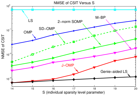
Figure 8: NMSE of CSIT versus the individual sparsity $s$ under $T=45$, $M=160$, $N=2$, $K=40$, $s_{c}=9$ and transmit SNR $P=28$ dB.

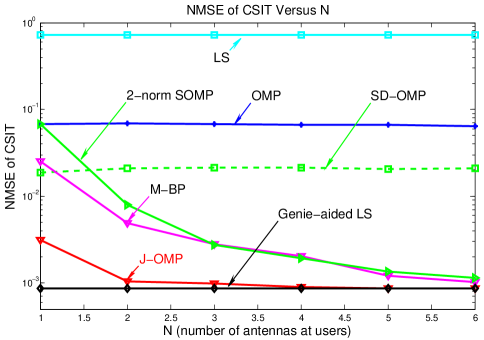
Figure 9: NMSE of CSIT versus the MS antennas $N$ under $T=45$, $M=160$, $K=40$, $s_{c}=9$, $s=17$ and transmit SNR $P=28$ dB.

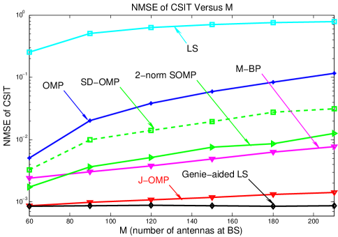
Figure 10: NMSE of CSIT versus the BS antennas $M$ under $T=45$, $N=2$, $K=40$, $s_{c}=9$, $s=17$ and transmit SNR $P=28$ dB.

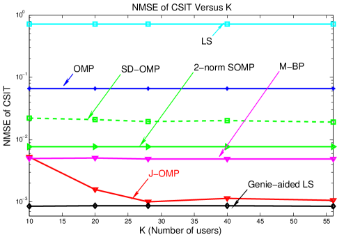
Figure 11: NMSE of CSIT versus the number of MSs $K$ under $T=45$, $M=160$, $N=2$, $s_{c}=9$, $s=17$ and transmit SNR $P=28$ dB.

V-D CSIT Estimation Quality Versus Individual Sparsity $s$

In Figure 8, we compare the NMSE of the estimated CSI versus the individual sparsity parameter $s$, under $T=45$, $M=160$, $N=2$, $K=40$, $s_{c}=9$ and $P=28$ dB. From this figure, we observe that the CSIT estimation quality gets worse as the individual sparsity level $s$ increases. This is because as the sparsity level ($s$) increases, larger number of measurements are needed according to the classical CS theory [17]. Hence, given the same CSIT estimation overhead $T$, the CSIT estimation performance decreases as the channel sparsity increases.

V-E CSIT Estimation Quality Versus MS Antennas $N$

In Figure 9, we compare the NMSE of the estimated CSI versus the MS antennas $N$, under $T=45$, $M=160$, $K=40$, $s_{c}=9$, $s=17$ and $P=28$ dB. From this figure, we observe that the CSIT estimation quality of the proposed scheme increases as $N$ increases. This is because the proposed J-OMP algorithm exploits the individual joint sparsity among the $N$ row vectors of each channel matrices. Hence, larger $N$ would have better CSIT estimation quality. This result also verifies Corollary 1 and shows that the proposed CSIT estimation scheme indeed exploits the individual joint sparsity (Corresponds to Observation I) of the user channel matrices to enhance the CSIT estimation performance.

V-F CSIT Estimation Quality Versus BS Antennas $M$

In Figure 10, we compare the NMSE of the estimated CSI versus the BS antennas $M$ under $T=45$, $N=2$, $K=40$, $s_{c}=9$, $s=17$ and $P=28$ dB. From this figure, the proposed J-OMP algorithm achieves better performance than the baselines. On the other hand, we observe that the CSIT estimation quality decreases as $M$ increases. This is because when the channel dimension (i.e., $M$) gets larger, larger CS measurements (i.e., a larger CSIT estimation overhead $T$) are needed from classical CS theory [17]. Conversely, given the same CSIT measurements (i.e., $T$), the CSIT estimation quality would decrease as $M$ increases.

V-G CSIT Estimation Quality Versus Number of MSs $K$

In Figure 11, we compare the NMSE of the estimated CSI versus the number of MSs $K$ under $T=45$, $M=160$, $N=2$, $s_{c}=9$, $s=17$ and $P=28$ dB. From this figure, we observe that the CSIT estimation quality of the proposed J-OMP scheme increases as $K$ increases. This is because the proposed J-OMP scheme exploits the distributed joint sparsity among the $K$ user channel matrices (Corresponds to the observation II) to jointly identify the common support (as in Algorithm 2). Hence, a larger $K$ would achieve better recovery of the common support and hence achieve a better CSIT estimation performance. This figure also verifies the derived result in Corollary 2.

V-H Comparison of Computation Complexity

In Table I, we compare the average computation time per link (in terms of seconds) under $T=45$, $N=2$, $K=40$, $s_{c}=9$, $s=17$ and $P=28$ dB. Three different cases are considered, namely the number of BS antennas $M=60$, $M=120$, and $M=180$. From this table, we observe that 1) The M-BP (mixed-norm basis pursuit) scheme, which is an optimization-based CS recovery algorithm [35, 36], has very high (the largest) computation complexity but it cannot beat the proposed J-OMP scheme (as in Figure 5-11) because the proposed J-OMP has exploited the joint sparsity structures among the user channel matrices to better recover the CSI; 2) All the greedy-based CS recovery schemes, including the proposed J-OMP, OMP, SOMP, SDOMP, have similar computation complexities, while the proposed J-OMP algorithm performs the best in Figure 5-11.

Computation Time (s)	$M=60$	$M=120$	$M=180$
Baseline1 (LS)	$4.9\times 10^{-5}$	$6.7\times 10^{-5}$	$8.1\times 10^{-5}$
Baseline2 (OMP)	$1.1\times 10^{-2}$	$1.5\times 10^{-2}$	$2.0\times 10^{-2}$
Baseline3 (SOMP)	$5.8\times 10^{-3}$	$8.1\times 10^{-3}$	$1.04\times 10^{-2}$
Baseline4 (M-BP)	$1.3$	$2.6$	$3.8$
Baseline5 (SDOMP)	$1.3\times 10^{-2}$	$1.6\times 10^{-2}$	$1.8\times 10^{-2}$
Proposed J-OMP	$5.4\times 10^{-3}$	$8.6\times 10^{-3}$	$1.2\times 10^{-2}$

TABLE I: Comparison of computation complexity in a multi-user massive network where $T=45$, $N=2$, $K=40$, $s_{c}=9$, $s=17$, $P=28$ dB and $M=60$,$120$, $180$.

VI Conclusion

In this paper, we consider multi-user massive MIMO systems and deploy the compressive sensing (CS) technique to reduce the training as well as the feedback overhead in the CSIT estimation. We propose a distributed compressive CSIT estimation scheme so that the compressed measurements are observed at the users locally, while the CSIT recovery is performed at the base station jointly. We develop joint OMP algorithm to conduct the CSIT reconstruction which exploits the joint sparsity in the user channel matrices. We also analyze the estimated CSIT equality in terms of the normalized mean absolute error, and we obtain simple insights into how the joint channel sparsity will contribute to enhancing the CSIT estimation quality in multi-user massive MIMO systems.

-A Proof of Theorem 1

We first have the following two lemmas (Lemma 1, 2).

Lemma 1

If event $\Theta_{a}$ implies event $\Theta_{b}$, then

$$\textrm{Pr}(\Theta_{a})\leq\textrm{Pr}\left(\Theta_{b}\right).$$ (27)

Proof:

Event $\Theta_{a}$ implies event $\Theta_{b}$ indicates that the event space of $\Theta_{a}$ is contained in the event space [44] of $\Theta_{b}$. Therefore, (27) is proved. ∎

Lemma 2

Suppose $x$ and $y$ are two random variables. The following inequality holds for any scalar $A$:

$$\Pr\left(x<y\right)\leq\Pr\left(x\leq A\right)+\Pr\left(y>A\right),$$

$$\textrm{Pr}\left(x+y\geq C\right)\leq\textrm{Pr}\left(x\geq C-A\right)+\textrm{Pr}\left(y>A\right).$$

Proof:

Note that ($x<y$) implies ($x\leq A$ or $y>A$), $(x+y\geq C)$ implies ($x\geq C-A$ or $y>A$) for any $A$. Based on this and from Lemma 1, Lemma 2 is proved. ∎

Based on the two lemmas, given event $\Lambda$, we then investigate the probability of event $\Theta_{c}$ w.r.t. to the randomness of the channel matrices for any given support profile $\mathcal{P}=\{\Omega_{c},\{\Omega_{i}:\forall i\}\}$. First note that event $\Theta_{c}$ happens if and only if each of the added indices in Step 2. B belong to $\Omega_{c}$. Denote $J$ as the current estimated common support in Step 2, then the next estimated $\Omega_{i}^{{}^{\prime}}(J)$ in Step 2. A, B is given by:

$$\Omega_{i}^{{}^{\prime}}(J) = \left\{j:\left\|(\bar{\mathbf{X}}(j))^{H}\left(\mathbf{I}-\mathbf{P}_{J}\right)\mathbf{\bar{Y}}_{i}\right\|_{F}^{2}\geq\eta_{1}N\right\}$$

$$\bigcap\arg\max_{\left|\Omega\right|=s-|J|}\left\|(\bar{\mathbf{X}}_{\Omega})^{H}\left(\mathbf{I}-\mathbf{P}_{J}\right)\mathbf{\bar{Y}}_{i}\right\|_{F}.$$

For the proposed J-OMP algorithm, we have the following 3 properties (Lemma 3-5).

Lemma 3

Denote $J$ as the current estimated common support in Step 2. Then any $l\subseteq J$ will not be picked again in the next estimated $\Omega_{i}^{{}^{\prime}}(J)$, i.e., $l\notin\Omega_{i}^{{}^{\prime}}(J)$.

Proof:

The lemma is proved by noting the following two equations:

$$\bar{\mathbf{X}}(l)^{H}\left(\mathbf{I}-\mathbf{P}_{J}\right)=0,\forall l\in J,$$ (29)

$$\bar{\mathbf{X}}(l)^{H}\left(\mathbf{I}-\mathbf{P}_{J}\right)\bar{\mathbf{Y}}_{i}\neq 0,\forall l\in[M]\backslash J,$$ (30)

where (30) holds almost surely due to the random noise term in $\bar{\mathbf{Y}}_{i}$. ∎

From Lemma 3, we obtain the following property:

Lemma 4

Denote $J\subseteq\Omega_{c}$, $|J|<s_{c}$, as the current estimated common support in Step 2. The next added index in Step 2. B will be belonging to $\Omega_{c}$ if $\mathcal{E}_{J}$ happens:

$$\mathcal{E}_{J}:\;\max_{l\in\Omega_{c}\backslash J}\sum_{i=1}^{K}I_{\{l\in\Omega_{i}^{{}^{\prime}}(J)\}}>\max_{j\in[M]\backslash\Omega_{c}}\sum_{i=1}^{K}I_{\{j\in\Omega_{i}^{{}^{\prime}}(J)\}}.$$ (31)

where $\Omega_{i}^{{}^{\prime}}(J)$ is given in (-A). ∎

From Lemma 4, we obtain the following lemma.

Lemma 5

Given $\Lambda$, to ensure that $\Theta_{c}$ happens, it suffices to require that $\mathcal{E}_{J}$ in (31) happens for all $J\subseteq\Omega_{c}$, $|J|<s_{c}$. ∎

Using the negative inverse proposition of Lemma 5 and from Lemma 1, we obtain

$$\textrm{Pr}(\bar{\Theta}_{c}\mid\Lambda)\leq\textrm{Pr}\left(\bigcup_{J\subseteq\Omega_{c},|J|<s_{c}}\mathcal{\bar{E}}_{J}\right)\leq\sum_{J\subseteq\Omega_{c},|J|<s_{c}}\textrm{Pr}\left(\mathcal{\bar{E}}_{J}\right),$$ (32)

where $\bar{\Theta}$ means the complement event of event $\Theta$. For a given $J\subseteq\Omega_{c},$ $|J|<s_{c}$ and $l\in\Omega_{c}\backslash J$, we obtain

$$\textrm{Pr}\left(\mathcal{\bar{E}}_{J}\right)\leq$$

$$\Pr\left(\sum_{i=1}^{K}I_{\{l\in\Omega_{i}^{{}^{\prime}}(J)\}}\leq\max_{j\in[M]\backslash\Omega_{c}}\sum_{i=1}^{K}I_{\{j\in\Omega_{i}^{{}^{\prime}}(J)\}}\right)$$

$$\overset{(a_{1})}{\leq}\Pr\left(\sum_{i=1}^{K}I_{\{l\in\Omega_{i}^{{}^{\prime}}(J)\}}\leq K_{1}\right)$$

$$+\Pr\left(\max_{j\in[M]\backslash\Omega_{c}}\sum_{i=1}^{K}I_{\{j\in\Omega_{i}^{{}^{\prime}}(J)\}}\geq K_{1}\right),$$ (33)

where $(a_{1})$ uses Lemma 2 and $K_{1}$ is a number that will be specified later. On the other hand, note that for any $j\in[M]\backslash\Omega_{c}$, from (14),

$$\sum_{i=1}^{K}I_{\{j\in\Omega_{i}^{{}^{\prime}}\}} = \sum_{i}I_{\{j\in\Omega_{i}^{{}^{\prime}},j\in\Omega_{i}\}}+\sum_{i}I_{\{j\in\Omega_{i}^{{}^{\prime}},j\notin\Omega_{i}\}}$$

$$\leq K_{o}+\sum_{i}I_{\{j\in\Omega_{i}^{{}^{\prime}},j\notin\Omega_{i}\}}.$$

Hence, we obtain

$$\Pr\left(\max_{j\in[M]\backslash\Omega_{c}}\sum_{i=1}^{K}I_{\{j\in\Omega_{i}^{{}^{\prime}}\}}\geq K_{1}\right)$$ (34)

$$\leq \Pr\left(\sum_{i=1}^{K}\max_{j\in[M]\backslash\Omega_{i}}I_{\{j\in\Omega_{i}^{{}^{\prime}}\}}\geq K_{1}-K_{o}\right).$$

We have the following results related to (33) and (34).

Lemma 6

For a given $J\subseteq\Omega_{c},$ $|J|<s_{c}$, $l\in\Omega_{c}\backslash J$, if $\theta>1,$ then the following probability bounds holds:

$$\Pr\left(I_{\{l\in\Omega_{i}^{{}^{\prime}}(J)\}}=0\right)\leq p,$$ (35)

$$\Pr\left(\max_{j\in[M]\backslash\Omega_{i}}I_{\{j\in\Omega_{i}^{{}^{\prime}}(J)\}}=1\right)\leq p,$$ (36)

where $\theta$ and $p$ are given in (1) and (16) respectively.

Proof:

See Appendix -B. ∎

First, $\left(\mathbf{\bar{H}}_{i}\right)^{\Omega_{i}}$, $\forall i$, are independent of each other and hence $I_{\{l\in\Omega_{i}^{{}^{\prime}}(J)\}}$ are independent of each other for different $i$. Second, denote $\{z_{i}\}_{i=1}^{K}$ as a series of i.i.d. Bernoulli random variables, with $\Pr(z_{i}=0)=p$ and $\Pr(z_{i}=1)=1-p$, $\forall i$. By comparing $\left\{I_{\{l\in\Omega_{i}^{{}^{\prime}}(J)\}}:\forall i\right\}$ with $\{z_{i}\}_{i=1}^{K}$, we obtain,

$$\Pr\left(\sum_{i=1}^{K}I_{\{l\in\Omega_{i}^{{}^{\prime}}(J)\}}\leq K_{1}\right)\leq\Pr\left(\sum_{i=1}^{K}z_{i}\leq K_{1}\right).$$

$$\quad=\sum_{t=0}^{K_{1}}\left(\begin{array}[]{c}K\\ t\end{array}\right)(1-p)^{t}p{}^{K-t}.$$ (39)

in (33). Similarly, we obtain

$$\Pr\left(\sum_{i=1}^{K}\max_{j\in[M]\backslash\Omega_{i}}I_{\{j\in\Omega_{i}^{{}^{\prime}}\}}\geq K_{1}-K_{o}\right)$$ (42)

$$\leq \sum_{t=0}^{K-K_{1}+K_{o}}\left(\begin{array}[]{c}K\\ t\end{array}\right)(1-p)^{t}p{}^{K-t}.$$

in (34). Choosing $K_{1}$ as $K_{1}=\left\lfloor\frac{K+K_{o}}{2}\right\rfloor$ and combining (33), (34), (39) and (42) together, Theorem 1 is proved.

-B Proof of Lemma 6

First, we introduce the following properties (43)-(45) from [45] which will be frequently used in the proof:

$$\bar{\mathbf{X}}\mathbf{\bar{H}}_{i}=\bar{\mathbf{X}}_{J}(\mathbf{\bar{H}}_{i})^{J}+\bar{\mathbf{X}}_{\Omega_{i}\backslash J}(\mathbf{\bar{H}}_{i})^{\Omega_{i}\backslash J},\forall J\subseteq\Omega_{i}.$$ (43)

$$\left(\mathbf{I}-\mathbf{P}_{J}\right)\bar{\mathbf{X}}_{J}=\mathbf{0},\;(\bar{\mathbf{X}}_{J})^{H}\left(\mathbf{I}-\mathbf{P}_{J}\right)=\mathbf{0}.$$ (44)

$$\left\|\mathbf{A}\mathbf{B}\right\|\leq\left\|\mathbf{A}\right\|\left\|\mathbf{B}\right\|,\;\left\|\mathbf{A}\mathbf{B}\right\|_{F}\leq\left\|\mathbf{A}\right\|\left\|\mathbf{B}\right\|_{F}.$$ (45)

Second, we have the following inequalities [31, 32] on the RIP property (Definition 2).

Lemma 7

For $J_{1},J_{2}\subseteq\Omega$, $|\Omega|=k$ and $J_{1}\bigcap J_{2}=\emptyset$,

$$\left\|(\bar{\mathbf{X}}_{J_{2}})^{H}\bar{\mathbf{X}}_{J_{1}}\right\|\leq\delta_{k}.$$ (46)

$$\left\|\left((\bar{\mathbf{X}}_{J_{1}})^{H}(\bar{\mathbf{X}}_{J_{1}})\right)^{-1}\right\|\leq\frac{1}{1-\delta_{k}}.$$ (47)

$$\left\|\bar{\mathbf{X}}_{\Omega}^{\dagger}\right\|\leq\frac{1}{\sqrt{1-\delta_{k}}}.$$ (48)

We prove Lemma 6 based on properties (43)-(48). Specifically, we first prove (35) and then prove (36) in a similar way. For a given $J\subseteq\Omega_{c},$ $|J|<s_{c}$, $l\in\Omega_{c}\backslash J$, we obtain

$$\Pr\left(I_{\{l\in\Omega_{i}^{{}^{\prime}}(J)\}}=0\right)\overset{(b_{1})}{\leq}\left(\left\|\bar{\mathbf{X}}(l)^{H}\left(\mathbf{I}-\mathbf{P}_{J}\right)\mathbf{\bar{Y}}_{i}\right\|_{F}^{2}<\eta_{1}N\right)$$ (49)

$$+\mbox{Pr}\left(\left\|\bar{\mathbf{X}}(l)^{H}\left(\mathbf{I}-\mathbf{P}_{J}\right)\mathbf{\bar{Y}}_{i}\right\|\leq\max_{j\in[M]\backslash\Omega_{i}}\left\|\bar{\mathbf{X}}(l)^{H}\left(\mathbf{I}-\mathbf{P}_{J}\right)\mathbf{\bar{Y}}_{i}\right\|\right)$$

where $(b_{1})$ comes from Lemma 1, and the fact that if both $\left\|\bar{\mathbf{X}}(l)^{H}\left(\mathbf{I}-\mathbf{P}_{J}\right)\mathbf{\bar{Y}}_{i}\right\|_{F}\geq\sqrt{\eta_{1}N}$ and

$$\left\|\bar{\mathbf{X}}(l)^{H}\left(\mathbf{I}-\mathbf{P}_{J}\right)\mathbf{\bar{Y}}_{i}\right\|>\max_{j\in[M]\backslash\Omega_{i}}\left\|\bar{\mathbf{X}}(l)^{H}\left(\mathbf{I}-\mathbf{P}_{J}\right)\mathbf{\bar{Y}}_{i}\right\|$$

hods, then we obtain $l\in\Omega_{i}^{{}^{\prime}}(J)$ according to (-A). On the other hand, we have the following inequality for the first term in (49):

$$\left\|\bar{\mathbf{X}}(l)^{H}\left(\mathbf{I}-\mathbf{P}_{J}\right)\mathbf{\bar{Y}}_{i}\right\|=$$ (50)

$$\left\|\bar{\mathbf{X}}(l)^{H}\left(\mathbf{I}-\mathbf{P}_{J}\right)\left(\bar{\mathbf{X}}_{J}\left(\bar{\mathbf{H}}_{i}\right)^{J}+\bar{\mathbf{X}}_{\Omega_{i}\backslash J}\left(\bar{\mathbf{H}}_{i}\right)^{\Omega_{i}\backslash J}+\mathbf{\bar{N}}_{i}\right)\right\|$$

$$\geq\left\|\bar{\mathbf{X}}(l)^{H}\left(\mathbf{I}-\mathbf{P}_{J}\right)\bar{\mathbf{X}}_{\Omega_{i}\backslash J}\left(\bar{\mathbf{H}}_{i}\right)^{\Omega_{i}\backslash J}\right\|-\sqrt{1+\delta_{1}}\left\|\mathbf{\bar{N}}_{i}\right\|_{F}$$

and the following for the second term in (49):

$$\left\|\bar{\mathbf{X}}(j)^{H}\left(\mathbf{I}-\mathbf{P}_{J}\right)\mathbf{\bar{Y}}_{i}\right\|$$ (51)

$$\leq\left\|\bar{\mathbf{X}}(j)^{H}\left(\mathbf{I}-\mathbf{P}_{J}\right)\bar{\mathbf{X}}_{\Omega_{i}\backslash J}\left(\bar{\mathbf{H}}_{i}\right)^{\Omega_{i}\backslash J}\right\|+\sqrt{1+\delta_{1}}\left\|\mathbf{\bar{N}}_{i}\right\|_{F}.$$

Based on (49)-(51) and using Lemma 2, we obtain

$$\Pr\left(I_{\{l\in\Omega_{i}^{{}^{\prime}}\}}=0\right)\leq\textrm{Pr}(\mathcal{D}_{i}^{[1]})+\textrm{Pr}(\mathcal{D}_{i}^{[2]})$$ (52)

$$+\textrm{Pr}(\mathcal{D}_{i}^{[3]})+\textrm{Pr}\left(\left\|\mathbf{\bar{N}}_{i}\right\|_{F}\geq\sqrt{\frac{MN\eta_{2}}{P}}\right)$$

$$\mathcal{D}_{i}^{[1]}:\quad\left\|\bar{\mathbf{X}}(l)^{H}\left(\mathbf{I}-\mathbf{P}_{J}\right)\bar{\mathbf{X}}_{\Omega_{i}\backslash J}\left(\bar{\mathbf{H}}_{i}\right)^{\Omega_{i}\backslash J}\right\|\leq\sqrt{N}\alpha,$$

$$\mathcal{D}_{i}^{[2]}:\quad\max_{j\in[M]\backslash\Omega_{i}}\left\|\bar{\mathbf{X}}(j)^{H}\left(\mathbf{I}-\mathbf{P}_{J}\right)\bar{\mathbf{X}}_{\Omega_{i}\backslash J}\left(\bar{\mathbf{H}}_{i}\right)^{\Omega_{i}\backslash J}\right\|$$

$$\geq\sqrt{N}\alpha-2\sqrt{\frac{\eta_{2}MN(1+\delta_{1})}{P}},$$

$$\mathcal{D}_{i}^{[3]}:\quad\left\|\bar{\mathbf{X}}(l)^{H}\left(\mathbf{I}-\mathbf{P}_{J}\right)\bar{\mathbf{X}}_{\Omega_{i}\backslash J}\left(\bar{\mathbf{H}}_{i}\right)^{\Omega_{i}\backslash J}\right\|$$

$$\leq\sqrt{\eta_{1}N}+\sqrt{\frac{\eta_{2}MN(1+\delta_{1})}{P}},$$

where $\eta_{2}>1$ and $\alpha$ is a scalar to be set later. Note that $\mathbf{\bar{N}}_{i}$ is i.i.d. complex Gaussian distributed with zero mean and variance $\frac{M}{PT}$. Therefore,

$$\textrm{Pr}\left(\left\|\mathbf{\bar{N}}_{i}\right\|_{F}\geq\sqrt{\frac{\eta_{2}MN}{P}}\right)=\textrm{Pr}\left(\chi_{2NT}\geq 2\eta_{2}NT\right)$$

where $\chi_{2NT}$ denotes chi-squared distributed with $2NT$ degrees of freedom. We further have the following 2 inequalities (53) and (54)) from Lemma 7: (i) for a given $J\subseteq\Omega_{c}$, $|J|<|\Omega_{c}|$, $l\in\Omega_{c}\backslash J$, we have

$$\left\|\bar{\mathbf{X}}(l)^{H}\left(\mathbf{I}-\mathbf{P}_{J}\right)\bar{\mathbf{X}}_{\Omega_{i}\backslash J}\right\|$$ (53)

$$\geq \left(\left\|\bar{\mathbf{X}}(l)^{H}\bar{\mathbf{X}}_{\Omega_{i}\backslash J}\right\|-\left\|\bar{\mathbf{X}}(l)^{H}\bar{\mathbf{X}}{}_{J}\left(\bar{\mathbf{X}}{}_{J}^{H}\bar{\mathbf{X}}_{J}\right)^{-1}\bar{\mathbf{X}}{}_{J}^{H}\bar{\mathbf{X}}_{\Omega_{i}\backslash J}\right\|\right)$$

$$\geq \left(1-\delta_{1}-\left\|\bar{\mathbf{X}}(l)^{H}\bar{\mathbf{X}}{}_{J}\right\|\left\|\left(\bar{\mathbf{X}}{}_{J}^{H}\bar{\mathbf{X}}_{J}\right)^{-1}\right\|\left\|\bar{\mathbf{X}}{}_{J}^{H}\bar{\mathbf{X}}_{\Omega_{i}\backslash J}\right\|\right)$$

$$\geq \left(\frac{1-2\delta_{s}}{1-\delta_{s}}\right),$$

and (ii) for $j\in[M]\backslash\Omega_{i}$,

$$\left\|\bar{\mathbf{X}}(j)^{H}\left(\mathbf{I}-\mathbf{P}_{J}\right)\bar{\mathbf{X}}_{\Omega_{i}\backslash J}\right\|$$ (54)

$$\leq \left\|\bar{\mathbf{X}}(j)^{H}\bar{\mathbf{X}}_{\Omega_{i}\backslash J}\right\|+$$

$$\left\|\bar{\mathbf{X}}(j)^{H}\bar{\mathbf{X}}_{J}\left((\bar{\mathbf{X}}{}_{J})^{H}\bar{\mathbf{X}}_{J}\right)^{-1}(\bar{\mathbf{X}}{}_{J})^{H}\bar{\mathbf{X}}_{\Omega_{i}\backslash J}\right\|$$

$$\leq \left(\delta_{s+1}+\frac{\delta_{s+1}\delta_{s}}{1-\delta_{s}}\right)\leq\left(\frac{\delta_{s+1}}{1-\delta_{s}}\right).$$

Recall from Definition 1 and (9) that $(\bar{\mathbf{H}}_{i})^{\Omega_{i}\backslash J}$ is i.i.d. complex Gaussian distributed with zero mean and unit variance. From (53), we obtain

$$\textrm{Pr}(\mathcal{D}_{i}^{[1]})\leq\Pr\left(\chi_{2N}\leq\frac{2N\alpha^{2}}{\left(\frac{1-2\delta_{s}}{1-\delta_{s}}\right)^{2}}\right).$$ (55)

$$\textrm{Pr}(\mathcal{D}_{i}^{[3]})\leq\Pr\left(\chi_{2N}\leq\frac{2N}{\theta}\right)$$

From (54), we obtain

$$\textrm{Pr}(\mathcal{D}_{i}^{[2]})\leq\sum_{j\notin\Omega_{i}}\cdot\Pr\left(\chi_{2N}\geq\frac{2N\left(\alpha-2\sqrt{\frac{\eta_{2}M(1+\delta_{1})}{P}}\right)^{2}}{\left(\frac{\delta_{s+1}}{1-\delta_{s}}\right)^{2}}\right).$$ (56)

For simplicity, we choose $\alpha\triangleq\sqrt{\left(\frac{\delta_{s+1}}{1-\delta_{s}}\right)+2\sqrt{\frac{\eta_{2}M(1+\delta_{1})}{P}}}\sqrt{\frac{1-2\delta_{s}}{1-\delta_{s}}}$. From $\theta>1$, we obtain $\alpha\geq\frac{\delta_{s+1}}{1-\delta_{s}}+2\sqrt{\frac{\eta_{2}M(1+\delta_{1})}{P}}$. Hence, from (56), we further obtain

$$\textrm{Pr}(\mathcal{D}_{i}^{[2]})\leq M\cdot\Pr\left(\chi_{2N}\geq\frac{2N\alpha^{2}}{\left(\frac{\delta_{s+1}}{1-\delta_{s}}+2\sqrt{\frac{\eta_{2}M(1+\delta_{1})}{P}}\right)^{2}}\right).$$ (57)

From (52), (55), (56) and (57),

$$\Pr\left(I_{\{l\in\Omega_{i}^{{}^{\prime}}\}}=0\right)\leq 2\cdot\Pr\left(\chi_{2N}\leq\frac{2N}{\theta}\right)$$ (58)

$$\qquad+M\cdot\Pr\left(\chi_{2N}\geq 2\theta N\right)+\textrm{Pr}\left(\chi_{2NT}\geq 2\eta_{2}NT\right).$$

Here, we would like to introduce the following inequalities from the Chernoff bounds theory [46]:

Lemma 8 (Chernoff Bounds)

Suppose $\chi_{2k}$ is chi-squared distributed with $2k$ degrees of freedom, we have the following bound

$$\Pr\left(\chi_{2k}\leq 2xk\right)\leq\exp\left(-k\left(-1+x-\ln x\right)\right),\;0<x<1.$$

$$\Pr\left(\chi_{2k}\geq 2xk\right)\leq\exp\left(-k\left(-1+x-\ln x\right)\right),\;x>1.$$

∎

Using the Chernoff bounds on (58), we obtain the following result which completes the proof of equation (35):

$$\Pr\left(I_{\{l\in\Omega_{i}^{{}^{\prime}}(J)\}}=0\right)\leq 2\exp\left(-N\left(\ln\theta+\frac{1}{\theta}-1\right)\right)+M\times$$

$$\exp\left(-N\left(\theta-\ln\theta-1\right)\right)+\exp\left(-NT\left(\eta_{2}-\ln\eta_{2}-1\right)\right)<p.$$

Next, we prove (36). First, we have

$$\Pr\left(\max_{j\in[M]\backslash\Omega_{i}}I_{\{j\in\Omega_{i}^{{}^{\prime}}(J)\}}=1\right)\overset{(b_{2})}{\leq}\textrm{Pr}\left(\vphantom{\min_{l\in\Omega_{i}\backslash J}\left\|\bar{\mathbf{X}}(l)^{H}\left(\mathbf{I}-\mathbf{P}_{J}\right)\mathbf{\bar{Y}}_{i}\right\|}\qquad\qquad\qquad\qquad\right.$$ (59)

$$\left.\max_{j\in[M]\backslash\Omega_{i}}\left\|\bar{\mathbf{X}}(j)^{H}\left(\mathbf{I}-\mathbf{P}_{J}\right)\mathbf{\bar{Y}}_{i}\right\|\geq\sqrt{\eta_{1}N}\right),$$

where $(b_{2})$ comes from Lemma 1 and the fact that

$$\max_{j\in[M]\backslash\Omega_{i}}\left\|\bar{\mathbf{X}}(j)^{H}\left(\mathbf{I}-\mathbf{P}_{J}\right)\mathbf{\bar{Y}}_{i}\right\|_{F}<\sqrt{\eta_{1}N}$$

would imply $\max_{j\in[M]\backslash\Omega_{i}}I_{\{j\in\Omega_{i}^{{}^{\prime}}\}}=0$ according to (-A). Based on (59), and similar to (52), we obtain

$$\Pr\left(\max_{j\in[M]\backslash\Omega_{i}}I_{\{j\in\Omega_{i}^{{}^{\prime}}(J)\}}=1\right)\leq$$ (60)

$$\Pr\left(\max_{j\in[M]\backslash\Omega_{i}}\left\|\bar{\mathbf{X}}(j)^{H}\left(\mathbf{I}-\mathbf{P}_{J}\right)\bar{\mathbf{X}}_{\Omega_{i}\backslash J}\left(\bar{\mathbf{H}}_{i}\right)^{\Omega_{i}\backslash J}\right\|\geq\right.$$

$$\left.\sqrt{\eta_{1}N}-\sqrt{\frac{\eta_{2}MN(1+\delta_{1})}{P}}\right)+\textrm{Pr}\left(\chi_{2NT}\geq 2\eta_{2}NT\right)$$

Based on (60), and similar to (56), we obtain

$$\Pr\left(\max_{j\in[M]\backslash\Omega_{i}}I_{\{j\in\Omega_{i}^{{}^{\prime}}\}}=1\right)\leq\exp\left(-NT\left(\eta_{2}-\ln\eta_{2}-1\right)\right)$$

$$+M\cdot\exp\left(-N\left(\theta-\ln\theta-1\right)\right)\leq p.$$

Therefore, (36) in Lemma 6 is proved.

-C Proof of Theorem 2

Given event $\Theta_{c}$ and $\Lambda$, we then investigate the probability that the estimated support for user $i$ is correct, i.e., $\Omega_{i}^{e}=\Omega_{i}$ (event $\Theta_{i}$). First, from (29), any selected index will not be selected again by Step 3. A. Hence, $\Theta_{i}\mid\Theta_{c}\Lambda$ happens if and only if for user $i$, Step 3 adds $|\Omega_{i}|-s_{c}$ new indices belonging to $\Omega_{i}$ and then stops. We first find a sufficient condition for event $\Theta_{i}$ to happen as follows:

Lemma 9 (Sufficient Conditions for $\Theta_{i}\mid\Theta_{c}\Lambda$)

If conditions $\mathcal{N}$, $\mathcal{S}$ holds and event $\mathcal{E}_{J}$ happens for all $J\subseteq\Omega_{i}$, $s_{c}\leq|J|<|\Omega_{i}|$, then event $\Theta_{i}\mid\Theta_{c}\Lambda$ will surely happen, where

$$\mathcal{N}:\quad\left\|\mathbf{\bar{N}}_{i}\right\|_{F}^{2}\leq\frac{\eta_{2}MN}{P},$$

$$\mathcal{S}:\quad\min_{l\in\Omega_{i}}||\left(\bar{\mathbf{H}}_{i}\right)^{\{l\}}||_{F}>\frac{2}{\sqrt{1-\delta_{s}}}\sqrt{\frac{\eta_{2}NM}{P}},$$ (61)

$$\mathcal{E}_{J}:\quad \max_{l\in\Omega_{i}\backslash J}\left\|\mathbf{\bar{X}}(l)^{H}\left(\mathbf{I}-\mathbf{P}_{J}\right)\mathbf{\bar{Y}}_{i}\right\|$$

$$>\max_{j\in[M]\backslash\Omega_{i}}\left\|\mathbf{\bar{X}}(j)^{H}\left(\mathbf{I}-\mathbf{P}_{J}\right)\mathbf{\bar{Y}}_{i}\right\|.$$

Proof:

We prove the lemma by following the procedures in Step 3. At first, the estimated support is $\Omega_{i}^{e}=\Omega_{c}^{e}\subseteq\Omega_{i}$ and $|\Omega_{i}^{e}|<|\Omega_{i}|$; then Step 3 will add a new support index instead of stopping for user $i$ because

$$\left\|\left(\mathbf{I}-\mathbf{P}_{\Omega_{i}^{e}}\right)\mathbf{\bar{Y}}_{i}\right\|_{F}$$

$$\overset{(c_{1})}{\geq} \left\|\left(\mathbf{I}-\bar{\mathbf{X}}_{\Omega_{i}^{e}}(\bar{\mathbf{X}}_{\Omega_{i}^{e}})^{\dagger}\right)\bar{\mathbf{X}}_{\Omega_{i}}\bar{\mathbf{H}}_{i}^{\Omega_{i}}\right\|_{F}-\sqrt{\frac{\eta_{2}NM}{P}}$$

$$\overset{(c_{2})}{=} \left\|\bar{\mathbf{X}}_{\Omega_{i}}\left(\bar{\mathbf{H}}_{i}^{a}-\bar{\mathbf{H}}_{i}\right)^{\Omega_{i}}\right\|_{F}-\sqrt{\frac{\eta_{2}NM}{P}}$$

$$\overset{(c_{3})}{\geq} \sqrt{1-\delta_{s}}\min_{l\in\Omega_{i}}||\left(\bar{\mathbf{H}}_{i}\right)^{\{l\}}||_{F}-\sqrt{\frac{\eta_{2}NM}{P}}$$

$$> \sqrt{\frac{\eta_{2}NM}{P}},$$

where $(c_{1})$ comes from condition $\mathcal{N}$; ($c_{2}$) comes from $\Omega_{i}^{e}\subseteq\Omega_{i}$ and $(\bar{\mathbf{H}}_{i}^{a})^{\Omega_{i}^{e}}=(\bar{\mathbf{X}}_{\Omega_{i}^{e}})^{\dagger}\bar{\mathbf{X}}_{\Omega_{i}}\bar{\mathbf{H}}_{i}^{\Omega_{i}}$, $(\bar{\mathbf{H}}_{i}^{a})^{[M]\backslash\Omega_{i}^{e}}=\mathbf{0}$; and $(c_{3})$ comes from $|\Omega_{i}^{e}|<|\Omega_{i}|$. On the other hand, from Step 3. A, the added index will be belonging to $\Omega_{i}\backslash\Omega_{i}^{e}$ as $\mathcal{E}_{J}$ holds for all $J$. Following the above procedures, Step 3 will continuously add indices that belong to $\Omega_{i}\backslash\Omega_{i}^{e}$ until $|\Omega_{i}^{e}|=|\Omega_{i}|$. Suppose Step 3 run into the case of $\Omega_{i}^{e}=\Omega_{i}$; then,

$$||\mathbf{R}_{i}||_{F}^{2}=\left\|\left(\mathbf{I}-\mathbf{P}_{\Omega_{i}}\right)\mathbf{\bar{N}}_{i}\right\|_{F}^{2}\leq\left\|\mathbf{\bar{N}}_{i}\right\|_{F}^{2}\leq\frac{\eta_{2}MN}{P}$$

and hence Step 3 stops for user $i$. Therefore, under the conditions in Lemma 9, event $\Theta_{i}$ conditioned on $\Theta_{c}$ and $\Lambda$ will surely happen. ∎

From Lemma 9 and Lemma 1, we obtain:

$$\textrm{Pr}(\bar{\Theta}_{i})\leq\textrm{Pr}\left(\min_{l\in\Omega_{i}}||\left(\bar{\mathbf{H}}_{i}\right)^{\{l\}}||_{F}\leq\frac{2\sqrt{\frac{\eta_{2}NM}{P}}}{\sqrt{1-\delta_{s}}}\right)$$ (63)

$$+\sum_{J\subseteq\Omega_{i},s_{c}\leq|J|<|\Omega_{i}|}\textrm{Pr}\left(\mathcal{\bar{E}}_{J}\right)+\textrm{Pr}\left(\left\|\mathbf{\bar{N}}_{i}\right\|_{F}^{2}>\frac{\eta_{2}MN}{P}\right).$$

First, we obtain

$$\textrm{Pr}\left(\min_{l\in\Omega_{i}}||\left(\bar{\mathbf{H}}_{i}\right)^{\{l\}}||_{F}\leq\frac{2\sqrt{\frac{\eta_{2}NM}{P}}}{\sqrt{1-\delta_{s}}}\right)$$ (64)

$$\leq \sum_{l\in\Omega_{i}}\textrm{Pr}\left(||\left(\bar{\mathbf{H}}_{i}\right)^{\{l\}}||_{F}^{2}\leq\frac{4\eta_{2}NM}{(1-\delta_{s})P}\right)$$

$$\leq s\cdot\textrm{Pr}\left(\chi_{2N}\leq\frac{8\eta_{2}NM}{(1-\delta_{s})P}\right)$$

$$\overset{(c_{4})}{\leq} s\exp\left(-N\left(\ln\vartheta+\frac{1}{\vartheta}-1\right)\right),$$

where $(c_{4})$ uses the Chernoff bounds in Lemma 8. Second, from Lemma 2, for a given $J\subseteq\Omega_{i},s_{c}\leq|J|<|\Omega_{i}|$:

$$\textrm{Pr}\left(\mathcal{\bar{E}}_{J}\right)\leq$$

$$\Pr\left(\max_{l\in\Omega_{i}\backslash J}\left\|\mathbf{\bar{X}}(l)^{H}\left(\mathbf{I}-\mathbf{P}_{J}\right)\mathbf{\bar{X}}_{\Omega_{i}\backslash J}\left(\bar{\mathbf{H}}_{i}\right)^{\Omega_{i}\backslash J}\right\|\leq\sqrt{N}\alpha\right)+$$

$$\Pr\left(\max_{j\in[M]\backslash\Omega_{i}}\left\|\mathbf{\bar{X}}(j)^{H}\left(\mathbf{I}-\mathbf{P}_{J}\right)\mathbf{\bar{X}}_{\Omega_{i}\backslash J}\left(\bar{\mathbf{H}}_{i}\right)^{\Omega_{i}\backslash J}\right\|\right.$$

$$\left.\geq\sqrt{N}\alpha-2\sqrt{\frac{\eta_{2}MN(1+\delta_{1})}{P}}\right).$$ (65)

From (53) and (54), and similar to the derivation in Appendix -B, we obtain

$$\textrm{Pr}\left(\mathcal{\bar{E}}_{J}\right)\leq\exp\left(-N\left(\ln\theta+\frac{1}{\theta}-1\right)\right)$$ (66)

$$+M\cdot\exp\left(-N\left(\theta-\ln\theta-1\right)\right).$$

Substituting (64) and (66) into (63), we obtain the desired theorem.

-D Proof of Theorem 3

First note that $\frac{\left\|\mathbf{H}_{i}-\mathbf{H}_{i}^{e}\right\|_{F}}{\left\|\mathbf{H}_{i}\right\|_{F}}=\frac{\left\|\mathbf{\bar{H}}_{i}-\mathbf{\bar{H}}^{e}\right\|_{F}}{\left\|\mathbf{\bar{H}}_{i}\right\|_{F}}$ and

$$\mathbb{E}\left(\frac{\left\|\mathbf{\bar{H}}_{i}-\mathbf{\bar{H}}^{e}\right\|_{F}}{\left\|\mathbf{\bar{H}}_{i}\right\|_{F}}\right)=\mathbb{E}\left(\frac{\left\|\mathbf{\bar{H}}_{i}-\mathbf{\bar{H}}^{e}\right\|_{F}}{\left\|\mathbf{\bar{H}}_{i}\right\|_{F}}\mid\bar{\Lambda}\right)\Pr(\bar{\Lambda})$$

$$+\mathbb{E}\left(\frac{\left\|\mathbf{\bar{H}}_{i}-\mathbf{\bar{H}}^{e}\right\|_{F}}{\left\|\mathbf{\bar{H}}_{i}\right\|_{F}}\mid\Theta_{i}\Theta_{c}\Lambda\right)\Pr(\Theta_{i}\Theta_{c}\Lambda)+$$

$$\mathbb{E}\left(\frac{\left\|\mathbf{\bar{H}}_{i}-\mathbf{\bar{H}}^{e}\right\|_{F}}{\left\|\mathbf{\bar{H}}_{i}\right\|_{F}}\mid\overline{\Theta_{i}\Theta_{c}}\Lambda\right)\Pr(\overline{\Theta_{i}\Theta_{c}}\mid\Lambda)\Pr\left(\Lambda\right).$$ (67)

Second,

$$\frac{\left\|\mathbf{\bar{H}}_{i}-\mathbf{\bar{H}}^{e}\right\|_{F}}{\left\|\mathbf{\bar{H}}_{i}\right\|_{F}}\leq\frac{\left\|\left(\bar{\mathbf{X}}_{\Omega_{i}^{e}}\right)^{\dagger}\mathbf{\bar{N}}_{i}\right\|_{F}}{\left\|\mathbf{\bar{H}}_{i}\right\|_{F}}+\frac{\left\|\mathbf{\bar{H}}_{i}^{\Omega_{i}\backslash\Omega_{i}^{e}}\right\|_{F}}{\left\|\mathbf{\bar{H}}_{i}\right\|_{F}}$$

$$+\frac{1}{\left\|\mathbf{\bar{H}}_{i}\right\|_{F}}\left\|\left(\bar{\mathbf{X}}_{\Omega_{i}^{e}}\right)^{\dagger}\bar{\mathbf{X}}_{\Omega_{i}\backslash\Omega_{i}^{e}}(\mathbf{\bar{H}}_{i})^{\Omega_{i}\backslash\Omega_{i}^{e}}\right\|_{F}$$ (68)

Note that $\left(\bar{\mathbf{X}}_{\Omega_{i}^{e}}\right)^{\dagger}$ contains at most $s$ non-zero singular values (i.e., $|\Omega_{i}^{e}|\leq s$) and each non-zero singular value is upper bounded by $\frac{1}{\sqrt{1-\delta_{s}}}$ from (48). Furthermore, $\mathbf{\bar{N}}_{i}$ and $(\mathbf{\bar{H}}_{i})^{\Omega_{i}}$ are i.i.d. complex Gaussian distributed (with variance $\frac{M}{PT}$ and $1$ respectively). Hence,

$$\mathbb{E}\left(\frac{\left\|\left(\bar{\mathbf{X}}_{\Omega_{i}^{e}}\right)^{\dagger}\mathbf{\bar{N}}_{i}\right\|_{F}}{\left\|(\mathbf{\bar{H}}_{i})^{\Omega_{i}}\right\|_{F}}\right)\leq\sqrt{\frac{2MsN}{PT(1-\delta_{s})}}\mathbb{E}\left((\chi_{2\tilde{s}_{i}N})^{-\frac{1}{2}}\right)\leq$$

$$\sqrt{\frac{2MsN}{PT(1-\delta_{s})}}\mathbb{E}\left((\chi_{2N})^{-\frac{1}{2}}\right)\leq\sqrt{\frac{MsN}{PT(1-\delta_{s})}}\frac{\Gamma\left(N-\frac{1}{2}\right)}{\Gamma\left(N\right)},$$

where $\chi_{2\tilde{s}_{i}N}$ denotes the chi-distribution with $2\tilde{s}_{i}N$ degrees of freedom, where $\tilde{s}_{i}\triangleq|\Omega_{i}|\geq 1$ from Definition 1. When $\Theta_{i}\Theta_{c}\Lambda$ happens, $\Omega_{i}=\Omega_{i}^{e}$, and hence $\mathbf{\bar{H}}_{i}^{\Omega_{i}\backslash\Omega_{i}^{e}}=\mathbf{0}$ in (68). Note that $\left\|\mathbf{\bar{H}}_{i}^{\Omega_{i}\backslash\Omega_{i}^{e}}\right\|_{F}\leq\left\|\mathbf{\bar{H}}_{i}\right\|_{F}$ always holds. When $\overline{\Theta_{i}\Theta_{c}}\mid\Lambda$ happens, from $\left\|\left(\bar{\mathbf{X}}_{\Omega_{i}^{e}}\right)^{\dagger}\bar{\mathbf{X}}_{\Omega_{i}\backslash\Omega_{i}^{e}}\right\|\leq\frac{\delta_{2s}}{1-\delta_{s}}$ according to Lemma 7, we obtain

$$\frac{1}{\left\|\mathbf{\bar{H}}_{i}\right\|_{F}}\left\|\left(\bar{\mathbf{X}}_{\Omega_{i}^{e}}\right)^{\dagger}\bar{\mathbf{X}}_{\Omega_{i}\backslash\Omega_{i}^{e}}(\mathbf{\bar{H}}_{i})^{\Omega_{i}\backslash\Omega_{i}^{e}}\right\|\leq\frac{\delta_{2s}}{1-\delta_{s}}$$ (69)

When $\bar{\Lambda}$ happens, from $\left\|\left(\bar{\mathbf{X}}_{\Omega_{i}^{e}}\right)^{\dagger}\right\|\leq\frac{1}{\sqrt{1-\delta_{s}}}$, $||\bar{\mathbf{X}}(j)||_{F}\leq\sqrt{1+\delta_{1}}$, $\forall j$, and the fact that $(\mathbf{\bar{H}}_{i})^{\Omega_{i}\backslash\Omega_{i}^{e}}$ are i.i.d. complex Gaussian distributed, we obtain

$$\mathbb{E}\left(\frac{\left\|\left(\bar{\mathbf{X}}_{\Omega_{i}^{e}}\right)^{\dagger}\bar{\mathbf{X}}_{\Omega_{i}\backslash\Omega_{i}^{e}}(\mathbf{\bar{H}}_{i})^{\Omega_{i}\backslash\Omega_{i}^{e}}\right\|_{F}}{\left\|\mathbf{\bar{H}}_{i}\right\|_{F}}\right)$$

$$\leq \frac{1}{\sqrt{1-\delta_{s}}}\mathbb{E}\left(\frac{\left\|\bar{\mathbf{X}}_{\Omega_{i}\backslash\Omega_{i}^{e}}(\mathbf{\bar{H}}_{i})^{\Omega_{i}\backslash\Omega_{i}^{e}}\right\|_{F}}{\left\|(\mathbf{\bar{H}}_{i})^{\Omega_{i}\backslash\Omega_{i}^{e}}\right\|_{F}}\right)\leq\sqrt{\frac{1+\delta_{1}}{1-\delta_{s}}}$$

Furthermore, we have $\Pr(\overline{\Theta_{i}\Theta_{c}}\mid\Lambda)\leq 2-\textrm{Pr}\left(\Theta_{i}\mid\Theta_{c}\Lambda\right)-\textrm{Pr}\left(\Theta_{c}\mid\Lambda\right)$. Substituting (68), (69) and (-D) into (67), we obtain the desired theorem.

-E Proof of Corollary 1

From (17), we obtain $C_{i}\leq g_{0}p^{\left\lfloor\frac{1-\gamma}{2}K\right\rfloor}$, where $g_{0}=2c_{0}\left(\frac{1-\delta_{s}+\delta_{2s}}{1-\delta_{s}}\right)\sum_{t=0}^{\left\lceil\frac{1+\gamma}{2}K\right\rceil}\left(\begin{array}[]{c}K\\ t\end{array}\right)$ which does not depend on $N$. Hence, from (16),

$$\lim_{N\rightarrow\infty}-\frac{1}{N}\ln\left(C_{i}\right)\geq\lim_{N\rightarrow\infty}-\left\lfloor\frac{1-\gamma}{2}K\right\rfloor\frac{\log p}{N}\geq\left\lfloor\frac{1-\gamma}{2}K\right\rfloor\beta_{1}.$$

On the other hand, (21) can be obtained from (18) similarly.

-F Proof of Corollary 2

From the large deviation result on Bernoulli random variables [44], we obtain the following Lemma:

Lemma 10

Suppose $0\leq p<1-\frac{K_{2}}{K}<1$, then

$$\lim_{K\rightarrow\infty}-\frac{1}{K}\ln\sum_{t=0}^{K_{2}}\left(\begin{array}[]{c}K\\ t\end{array}\right)(1-p)^{t}p^{K-t}$$ (73)

$$\quad=\left(1-\frac{K_{2}}{K}\right)\ln\frac{p(K-K_{2})}{K_{2}(1-p)}-\ln\frac{Kp}{K_{2}}>0.$$ (74)

Proof:

Suppose that $\{z_{i}\}_{i=1}^{M}$ is a series of i.i.d. Bernoulli random variables with $\Pr(z_{i}=1)=p$ and $\Pr(z_{i}=0)=1-p$, $\forall i$. We have

$$\lim_{K\rightarrow\infty}-\frac{1}{K}\ln\sum_{t=0}^{K_{2}}\left(\begin{array}[]{c}K\\ t\end{array}\right)(1-p)^{t}p^{K-t}$$

$$= \lim_{K\rightarrow\infty}-\frac{1}{K}\ln\Pr\left(\sum_{i=1}^{K}z_{i}\geq K-K_{2}\right)$$

$$\overset{(e_{1})}{=} \sup_{\epsilon>0}\left(\frac{(K-K_{2})\epsilon}{K}-\mathbb{E}\ln\left(\exp\left(\epsilon z_{i}\right)\right)\right)$$ (78)

where $(e_{1})$ is from the large deviation theory [44] and (78) can be easily simplified to be (74). ∎

Substituting the lower bound of $\textrm{Pr}(\Theta_{c}\mid\Lambda)$ in Theorem 1 into (3) and further using Lemma 10 with $K_{2}=\left\lceil\frac{1+\gamma}{2}K\right\rceil$, we obtain Corollary 2.

References

- [1] E. Telatar, “Capacity of multi-antenna gaussian channels,” Euro. Trans. Telecommun., vol. 10, no. 6, pp. 585–595, 1999.
- [2] E. G. Larsson, F. Tufvesson, O. Edfors, and T. L. Marzetta, “Massive MIMO for next generation wireless systems,” arXiv preprint arXiv:1304.6690, 2013. [Online]. Available: http://arxiv.org/abs/1304.6690
- [3] Q. Shi, M. Razaviyayn, Z.-Q. Luo, and C. He, “An iteratively weighted mmse approach to distributed sum-utility maximization for a MIMO interfering broadcast channel,” IEEE Trans. Signal Process., vol. 59, no. 9, pp. 4331–4340, 2011.
- [4] T. E. Bogale and L. Vandendorpe, “Weighted sum rate optimization for downlink multiuser MIMO coordinated base station systems: Centralized and distributed algorithms,” IEEE Trans. Signal Process., vol. 60, no. 4, pp. 1876–1889, 2012.
- [5] J. Hoydis, S. ten Brink, and M. Debbah, “Massive MIMO in the UL/DL of cellular networks: How many antennas do we need?” IEEE J. Sel. Areas Commun., vol. 31, no. 2, pp. 160–171, 2013.
- [6] S. L. H. Nguyen and A. Ghrayeb, “Compressive sensing-based channel estimation for massive multiuser MIMO systems,” in Proc. IEEE Wireless Commun. Networking Conf. (WCNC). IEEE, 2013, pp. 2890–2895.
- [7] P. W. Chan, E. S. Lo, R. R. Wang, E. K. Au, V. K. Lau, R. S. Cheng, W. H. Mow, R. D. Murch, and K. B. Letaief, “The evolution path of 4g networks: FDD or TDD?” IEEE Commun. Mag., vol. 44, no. 12, pp. 42–50, 2006.
- [8] T. L. Marzetta, G. Caire, M. Debbah, I. Chih-Lin, and S. K. Mohammed, “Special issue on massive MIMO,” Journal of Commun. and Networks, vol. 15, no. 4, pp. 333–337, 2013.
- [9] Q. Sun, D. C. Cox, H. C. Huang, and A. Lozano, “Estimation of continuous flat fading MIMO channels,” IEEE Trans. Wireless Commun., vol. 1, no. 4, pp. 549–553, 2002.
- [10] M. Biguesh and A. B. Gershman, “Training-based MIMO channel estimation: a study of estimator tradeoffs and optimal training signals,” IEEE Trans. Signal Process., vol. 54, no. 3, pp. 884–893, 2006.
- [11] H. Yin, D. Gesbert, M. Filippou, and Y. Liu, “A coordinated approach to channel estimation in large-scale multiple-antenna systems,” IEEE J. Sel. Areas Commun., vol. 31, no. 2, pp. 264–273, 2013.
- [12] Y. Zhou, M. Herdin, A. M. Sayeed, and E. Bonek, “Experimental study of MIMO channel statistics and capacity via the virtual channel representation,” Univ. Wisconsin-Madison, Madison, Tech. Rep., Feb 2007.
- [13] P. Kyritsi, D. C. Cox, R. A. Valenzuela, and P. W. Wolniansky, “Correlation analysis based on MIMO channel measurements in an indoor environment,” IEEE J. Sel. Areas Commun., vol. 21, no. 5, pp. 713–720, 2003.
- [14] F. Kaltenberger, D. Gesbert, R. Knopp, and M. Kountouris, “Correlation and capacity of measured multi-user MIMO channels,” in Proc. IEEE Int. Symp. Personal, Indoor and Mobile Radio Commun. (PIMRC), 2008, pp. 1–5.
- [15] J. Hoydis, C. Hoek, T. Wild, and S. ten Brink, “Channel measurements for large antenna arrays,” in Proc. IEEE Int. Symp. Wireless Commun. Systems (ISWCS), 2012, pp. 811–815.
- [16] X. Gao, O. Edfors, F. Rusek, and F. Tufvesson, “Linear pre-coding performance in measured very-large MIMO channels,” in Proc. IEEE Vehicular Technology Conf. (VTC), 2011, pp. 1–5.
- [17] C. R. Berger, Z. Wang, J. Huang, and S. Zhou, “Application of compressive sensing to sparse channel estimation,” IEEE Commun. Mag., vol. 48, no. 11, pp. 164–174, 2010.
- [18] W. U. Bajwa, J. Haupt, A. M. Sayeed, and R. Nowak, “Compressed channel sensing: A new approach to estimating sparse multipath channels,” Proceedings of the IEEE, vol. 98, no. 6, pp. 1058–1076, 2010.
- [19] J. Poutanen, K. Haneda, J. Salmi, V. Kolmonen, F. Tufvesson, T. Hult, and P. Vainikainen, “Significance of common scatterers in multi-link indoor radio wave propagation,” in Proc. IEEE European Conf. Antennas and Propagation (EuCAP), 2010, pp. 1–5.
- [20] Y. Barbotin, A. Hormati, S. Rangan, and M. Vetterli, “Estimation of sparse MIMO channels with common support,” IEEE Trans. Commun., vol. 60, no. 12, pp. 3705–3716, Dec. 2012.
- [21] D. Baron, M. F. Duarte, M. B. Wakin, S. Sarvotham, and R. G. Baraniuk, “Distributed compressive sensing,” arXiv preprint arXiv:0901.3403, 2005. [Online]. Available: http://arxiv.org/abs/0901.3403
- [22] J. Chen and X. Huo, “Theoretical results on sparse representations of multiple-measurement vectors,” IEEE Trans. Signal Process., vol. 54, no. 12, pp. 4634–4643, 2006.
- [23] R. Gribonval, H. Rauhut, K. Schnass, and P. Vandergheynst, “Atoms of all channels, unite! average case analysis of multi-channel sparse recovery using greedy algorithms,” Journal of Fourier analysis and Applications, vol. 14, no. 5-6, pp. 655–687, 2008.
- [24] Y. C. Eldar and H. Rauhut, “Average case analysis of multichannel sparse recovery using convex relaxation,” IEEE Trans. Inf. Theory, vol. 56, no. 1, pp. 505–519, 2010.
- [25] A. Scaglione and A. Vosoughi, “Turbo estimation of channel and symbols in precoded MIMO systems,” in Proc. IEEE Int. Conf. Acoustics, Speech, Signal Processing (ICASSP), vol. 4, 2004, pp. iv413–iv416.
- [26] D. Tse and P. Viswanath, Fundamentals of wireless communication. Cambridge Univ Pr, 2005.
- [27] L. Bottou and N. Murata, “Stochastic approximations and efficient learning,” The Handbook of Brain Theory and Neural Networks, Second edition,. The MIT Press, Cambridge, MA, 2002.
- [28] C. Berger, S. Zhou, J. Preisig, and P. Willett, “Sparse channel estimation for multicarrier underwater acoustic communication: From subspace methods to compressed sensing,” IEEE Trans. Signal Process., vol. 58, no. 3, pp. 1708–1721, 2010.
- [29] E. Candes and T. Tao, “Decoding by linear programming,” IEEE Trans. Inf. Theory, vol. 51, no. 12, pp. 4203–4215, 2005.
- [30] J. A. Tropp and A. C. Gilbert, “Signal recovery from random measurements via orthogonal matching pursuit,” IEEE Trans. Inf. Theory, vol. 53, no. 12, pp. 4655–4666, 2007.
- [31] D. Needell and J. A. Tropp, “Cosamp: Iterative signal recovery from incomplete and inaccurate samples,” Applied and Computational Harmonic Analysis, vol. 26, no. 3, pp. 301–321, 2009.
- [32] W. Dai and O. Milenkovic, “Subspace pursuit for compressive sensing signal reconstruction,” IEEE Trans. Inf. Theory, vol. 55, no. 5, pp. 2230–2249, 2009.
- [33] M. F. Duarte and Y. C. Eldar, “Structured compressed sensing: From theory to applications,” IEEE Trans. Signal Process., vol. 59, no. 9, pp. 4053–4085, 2011.
- [34] J. A. Tropp, A. C. Gilbert, and M. J. Strauss, “Algorithms for simultaneous sparse approximation. part I: Greedy pursuit,” Signal Processing, vol. 86, no. 3, pp. 572–588, 2006.
- [35] Y. C. Eldar and M. Mishali, “Robust recovery of signals from a structured union of subspaces,” IEEE Trans. Inf. Theory, vol. 55, no. 11, pp. 5302–5316, 2009.
- [36] J. A. Tropp, “Algorithms for simultaneous sparse approximation. part II: Convex relaxation,” Signal Processing, vol. 86, no. 3, pp. 589–602, 2006.
- [37] J. Liang, Y. Liu, W. Zhang, Y. Xu, X. Gan, and X. Wang, “Joint compressive sensing in wideband cognitive networks,” in Proc. IEEE Wireless Commun. Networking Conf. (WCNC), 2010, pp. 1–5.
- [38] R. G. Baraniuk, V. Cevher, M. F. Duarte, and C. Hegde, “Model-based compressive sensing,” IEEE Trans. Inf. Theory, vol. 56, no. 4, pp. 1982–2001, 2010.
- [39] E. J. Candès and M. B. Wakin, “An introduction to compressive sampling,” IEEE Signal Process. Mag., vol. 25, no. 2, pp. 21–30, 2008.
- [40] G. Sideratos and N. D. Hatziargyriou, “An advanced statistical method for wind power forecasting,” IEEE Trans. Power Systems, vol. 22, no. 1, pp. 258–265, 2007.
- [41] J. Flum and M. Grohe, Parameterized complexity theory. Springer, 2006, vol. 3.
- [42] G. T. 25.996, “Universal mobile telecommunications system (umts); spacial channel model for multiple input multiple output (mimo) simulations,” 3GPP ETSI Release 9, Tech. Rep., 2010. [Online]. Available: http://www.3gpp.org/DynaReport/25996.htm
- [43] M. Klessling, J. Speidel, and Y. Chen, “MIMO channel estimation in correlated fading environments,” in Proc. IEEE Vehicular Technology Conf. (VTC), vol. 2, 2003, pp. 1187–1191.
- [44] S. R. Varadhan, “Large deviations and applications,” in École d’Été de Probabilités de Saint-Flour XV–XVII, 1985–87. Springer, 1988, pp. 1–49.
- [45] D. Bernstein, Matrix mathematics: theory, facts, and formulas. Princeton University Press, 2011.
- [46] S. Dasgupta and A. Gupta, “An elementary proof of a theorem of johnson and lindenstrauss,” Random Structures & Algorithms, vol. 22, no. 1, pp. 60–65, 2003.