Highly Accreting Quasars: Sample Definition and Possible Cosmological Implications

Abstract

We propose a method to identify quasars radiating closest to the Eddington limit, defining primary and secondary selection criteria in the optical, UV and X-ray spectral range based on the 4D eigenvector 1 formalism. We then show that it is possible to derive a redshift-independent estimate of luminosity for extreme Eddington ratio sources. Using preliminary samples of these sources in three redshift intervals (as well as two mock samples), we test a range of cosmological models. Results are consistent with concordance cosmology but the data are insufficient for deriving strong constraints. Mock samples indicate that application of the method proposed in this paper using dedicated observations would allow to set stringent limits on $\Omega_{\mathrm{M}}$ and significant constraints on $\Omega_{\Lambda}$.

1 Introduction

The concordance cosmology model (Spergel et al., 2003; Riess et al., 2009; Komatsu et al., 2011) favors a flat Universe ($\Omega_{\mathrm{M}}$+ $\Omega_{\Lambda}$=1) and significant energy density associated with a cosmological constant ($\Omega_{\Lambda}$=0.72). Inference of a significantly non-zero $\Omega_{\Lambda}$ rests on the use of supernovæ as standard candles (Perlmutter et al., 1997, 1999) and studies of the cosmic microwave background radiation (e.g. Tegmark et al., 2004). The most recent Wilkinson Microwave Anisotropy Probe (WMAP) results indicate that the baryonic acoustic oscillation scale, the Hubble constant and the densities are determined to a precision of $\approx$1.5% (Hinshaw et al., 2012). Even if the large-scale distribution of galaxies (Schlegel et al., 2011; Nuza et al., 2012) and galaxy clusters (e.g., Allen et al., 2011) provide additional constraints, it is urgent that independent lines of investigation are devised to test these results. It remains important because $\Omega_{\mathrm{M}}$ is not very tightly constrained by supernova surveys (Conley et al., 2011): $\Omega_{\mathrm{M}}$$\;\buildrel<\over{\sim}\;$0.5 at 2-$\sigma$ confidence level from supernovæ mainly at $z\lower 2.15277pt\hbox{$\;\buildrel<\over{\sim}\;$}$ 1.5 (Campbell et al., 2013). Little information on $\Omega_{\mathrm{M}}$ has been extracted from the redshift range $1\lower 2.15277pt\hbox{$\;\buildrel<\over{\sim}\;$}z\lower 2.15277pt\hbox{$\;\buildrel<\over{\sim}\;$}3$, where $\Omega_{\mathrm{M}}$ is most strongly affecting the metric. In addition, recently announced cosmological parameter values from the Planck-only best-fit 6-parameter $\Lambda$-cold dark matter model differ from the previous WMAP estimate, and yield $\Omega_{\Lambda}$=0.69$\pm$0.01 (Planck Collaboration et al., 2013), significantly different from $\Omega_{\Lambda}$= 0.72, $\Omega_{\mathrm{M}}$=0.28 of the concordance cosmology adopted in the past few years (Hinshaw et al., 2009).

It is perhaps appropriate that we reconsider the cosmological utility of quasars at the fiftieth anniversary of their discovery (e.g., D’Onofrio et al., 2012). It is well known that use of quasar properties for independent measurement of cosmological parameters is fraught with difficulties. Quasars show properties that make them potential cosmological probes (see e.g. Bartelmann et al. 2009): they are plentiful, very luminous, and detected at early cosmic epochs (currently out to $z\approx 7$, Mortlock et al. 2011). The downside is that they show a more than 6dex spread in luminosity and are also anisotropic radiators. Quasars are thought to be the observational manifestation of accretion onto super-massive black holes. Accretion phenomena in the Universe show a scale invariance with respect to mass and, indeed, we observe similar quasar spectra over the entire luminosity/mass range. It is not surprising that pre-1990 quasar research tacitly assumed that high and low luminosity active galactic nuclei (AGN) were spectroscopically similar as well. The key to possible cosmological utility lies in realizing that quasars show a wide dispersion in observational properties which is a reflection of the source Eddington ratio.

1.1 Quasar Systematics

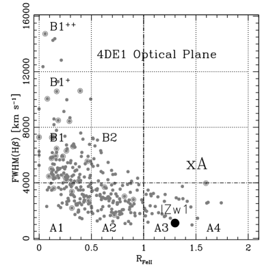
Figure 1: The optical plane of the 4DE1 space, FWHM H$\beta$ vs $R_{\rm FeII}$. Data points (in grey) are from the sample of Zamfir et al. (2010); circled points represent RL sources. The plane is binned following Sulentic et al. (2002) to identify spectral types (thin dot-dashed lines). The thick dot-dashed line separates extreme Pop. A source by the criterion $R_{\rm FeII}$$\geq$1.0. The large filled circle identifies the extreme Pop. A source I Zw 1.

The goal of systematizing observational properties of quasars has made considerable progress in the past 20 years and this makes possible discrimination of sources by $L/L_{\mathrm{Edd}}$. An important first step involved a principal component analysis of line profile measures from high S/N spectra of 87 PG quasars (Boroson & Green, 1992). That study revealed of Eigenvector 1 (E1) correlates including a trend of increasing optical Feii emission strength with decreasing FWHM H$\beta$ and peak intensity of [Oiii]$\lambda$5007. Source luminosity was found to be part of the second Eigenvector and is therefore not directly correlated with the Eigenvector 1 parameters. A second step in quasar systematization attempted to identify more key line and continuum diagnostic measures. 4D Eigenvector 1 (4DE1, Sulentic et al., 2000a) included two E1 broad line measures: 1) full width half maximum of broad H$\beta$ (FWHM H$\beta$) and 2) optical Feii strength defined by the equivalent width W or by the intensity ratio $R_{\rm FeII}$= W(Feii$\lambda$4570)/W(H$\beta$) $\approx$ $I$(Feii$\lambda$4570)/$I$(H$\beta$), where Feii$\lambda$4570 indicates the blend of Feii emission between 4434 Å and 4684 Å. Figure 1 shows the optical plane of 4DE1 as defined by the 470 brightest quasars from SDSS DR5. Domain space in the figure is binned in such a way that all sources within a bin are the same within measurement uncertainties, and can be assigned a well-defined spectral type (Sulentic et al., 2002; Zamfir et al., 2010). The majority of quasars occupy bins A2 and B1 with tails extending towards bins with sources showing stronger Feii emission or broader H$\beta$ profiles. Currently eight bins in intervals of FWHM = 4000 km s^-1 and $R_{\rm FeII}$= 0.5 are needed to fully map source occupation. 4DE1 added two additional principal parameters: 3) a measure discussed in Wang et al. (1996) of the soft X-ray photon index ($\Gamma_{\mathrm{soft}}$) and 4) a measure of the Civ$\lambda$1549 broad line profile shift (at half maximum, Sulentic et al., 2007). Points of departure from BG92 involve: a) removal of [Oiii]$\lambda$5007 measures as 4DE1 correlates, b) consideration of differences in parameter space occupation between radio-quiet (RQ) and radio-loud (RL) sources (Sulentic et al., 2003; Zamfir et al., 2008) as well as c) division of sources into two populations (A and B) designed to emphasize source spectroscopic differences.

Population A sources show FWHM H$\beta<$4000 km s^-1, stronger $R_{\rm FeII}$, a soft X-ray excess and Civ$\lambda$1549 blueshift/asymmetry. Pop. A includes sources often called Narrow line Seyfert 1s (NLSy1s). The H$\beta$ broad-line profile shows an unshifted Lorentzian shape (Véron-Cetty et al., 2001). Population B sources show FWHM H$\beta>$4000 km s^-1 with weaker $R_{\rm FeII}$, no soft X-ray excess and usually no Civ$\lambda$1549 blueshift. Most RL sources are found in the Pop. B domain of Figure 1. Pop. B sources usually require a double Gaussian model (broad unshifted + very broad redshifted components) to describe H$\beta$. Labels on the bins shown in Figure 1 identify regions of occupation for the two source populations following the spectral type classification of Sulentic et al. (2002). Other important 4DE1 correlates exist. The present 4DE1 parameters represent those for which large numbers of reasonably accurate measures are available and for which clear correlations can be seen.

4DE1 parameters measure: FWHM H$\beta$ – the dispersion in low ionization line broad line region (BLR) gas velocity (it is the virial estimator of choice at low $z$), $R_{\rm FeII}$ – the relative strengths of Feii and H$\beta$ emission–likely driven by density $n_{\mathrm{H}}$, ionization and metallicity, $\Gamma_{\mathrm{soft}}$ – the strength of a soft X-ray excess viewed as a thermal signature of accretion (Shields, 1978; Malkan & Sargent, 1982) and Civ$\lambda$1549 shift – the amplitude of systemic radial motions in high ionization BLR gas, possibly due to an accretion disk wind (Konigl & Kartje, 1994; Proga, 2003; Königl, 2006). If we ask what might drive the source distribution in Figure 1 (or any of the other planes of 4DE1) , the answer is most likely Eddington ratio. The idea that Eddington ratio drives 4DE1 goes back to the first E1 study (Boroson & Green, 1992) and has received considerable support in the past 20 years (e.g., Boroson, 2002; Marziani et al., 2003c; Baskin & Laor, 2004; Grupe, 2004; Yip et al., 2004; Ai et al., 2010; Wang et al., 2011; Matsuoka, 2012; Xu et al., 2012). Black hole mass, and orientation are sources of scatter in the 4DE1 sequence. The value $L/L_{\rm Edd}$ $\approx$ 0.2$\pm$0.1 corresponds to the boundary between Pop. A and B sources (for a black hole mass $\log$ $M_{\rm BH}$ $\sim$ 8.0, Marziani et al., 2001, 2003c), and may be ultimately related to a transition between a geometrically thin, optically thick disk and an advection dominated, “slim” disk (e.g., Różańska & Czerny, 2000; Collin et al., 2002; Chen & Wang, 2004). Identification of the most extreme accretors (potentially “Eddington standard candles”) offers the best hope toward finding a cosmologically useful sample of quasars.

1.2 Finding “Eddington Standard Candles”

Any attempt to use quasars as redshift-independent distance estimators must be tied to identification of a special class with some well-defined observational properties. These properties should be chosen to provide an easy link to a physical parameter related to source luminosity. If $L/L_{\rm Edd}$ is known then standard assumptions can lead to a $z$-independent estimate of source luminosity since source luminosity estimation is connected to estimation of $M_{\rm BH}$ (§3).

Empirical studies show that the $L/L_{\rm Edd}$ distribution truncates near $L/L_{\rm Edd}$ $\approx$1 (e.g., Woo & Urry, 2002; Shen et al., 2011). We observe a few super–Eddington outliers but their masses have likely been significantly underestimated due to a special line-of-sight orientation (e.g. sources oriented face-on where virial motions make little or no contribution to line width Marziani et al. 2003c and Marziani & Sulentic 2012). The range of $L/L_{\rm Edd}$ is $0.01\la$$L/L_{\rm Edd}$$\la 1$ for luminous Seyfert 1 nuclei and quasars (Woo & Urry, 2002; Marziani et al., 2003c; Steinhardt & Elvis, 2010; Shen & Kelly, 2012) with a much broader range if low-luminosity sources (of less interest for the present study) are included. The flux-limited distribution of $L/L_{\rm Edd}$ is subject to a strong, mass dependent Malmquist bias (Shen & Kelly, 2012) that may explain claims of a significantly narrower range. The minimum detectable $L/L_{\rm Edd}$ for a limiting magnitude $m_{\mathrm{B,lim}}$ can be written as $L/L_{\rm{Edd,min}}\propto\frac{1}{M_{\rm{BH}}}10^{-0.4m_{\mathrm{B,lim}}}f(z)^{2}(1+z)^{(1-a)}$, where $f(z)$ is the redshift function appearing in the comoving distance definition, and $a$ is the visual continuum spectral index. The above expression shows that only lower $L/L_{\rm Edd}$ values are lost at increasing redshift and that the effect is $M_{\rm BH}$-dependent.

A physical motivation underlies our search for sources radiating at extreme Eddington ratio. When accretion becomes super-Eddington, emitted radiation is advected toward the black hole, so that the source luminosity tends to saturate if accretion rate $\dot{m}\gg\dot{m}_{\mathrm{Edd}}$, where $\dot{m}_{\mathrm{Edd}}=L_{\mathrm{Edd}}/\eta c^{2}$ is the Eddington accretion rate for fixed efficiency. The parameter $\eta$ can be assumed $\approx\frac{1}{6}$, as for $\alpha$ accretion disks (e.g., Shakura & Sunyaev, 1973), or equal 1 (Mineshige et al., 2000). Radiative efficiency is expected to decrease with increasing Eddington ratio and luminosity to increase with log accretion rate (Abramowicz et al., 1988; Szuszkiewicz et al., 1996; Collin & Kawaguchi, 2004; Kawaguchi et al., 2004). Current models indicate a saturation value of a few times the Eddington luminosity for the bolometric luminosity (Mineshige et al., 2000; Watarai et al., 2000). The observed $L/L_{\rm Edd}$ distribution of high Eddington ratio candidates considered in this paper is consistent with a limiting $L/L_{\rm Edd}$$\rightarrow 1$ (§2.3), as found in earlier empirical (e.g., Marziani et al., 2003c).

The primary goal of this paper is to find sources radiating near the limit $L/L_{\rm Edd}$  using emission line intensity ratios. These sources should be the quasars most easily found in flux-limited surveys i.e., the bias described above will only result in selective loss of quasars radiating at lower Eddington ratios for fixed $M_{\rm BH}$. We suggest that the 4DE1 formalism provides a set of parameters currently best suited to identify extreme Eddington radiators (§2). A second goal is to propose a method to for using high $L/L_{\rm Edd}$ quasars as redshift-independent luminosity estimators where the constant parameter is Eddington ratio rather than luminosity (§3). We report explorative calculations and preliminary results (§4) and discuss possible improvements (§5) along with limits and uncertainties (§6).

2 Sample Selection and Measurements

2.1 I Zw 1 as a prototype of highly accreting quasars

The much studied NLSy1 source I Zw 1 is considered to be a low-$z$  ($z\approx 0.0605$) prototype of quasars radiating close to the Eddington limit. It is located in bin A3 of Figure 1. The 4DE1 properties of I Zw 1 are:

1. FWHM H$\beta$= 1200$\pm$50 km s^-1 (Boroson & Green, 1992);

2. $R_{\rm FeII}$= 1.3$\pm$0.1 (Boroson & Green, 1992);

3. Civ$\lambda$1549 blueshift at FWHM (relative to rest frame) $\Delta$ $v_{\mathrm{r}}$= -1670$\pm$100 km s^-1(Sulentic et al., 2007);

4. soft-X photon index $\Gamma_{\mathrm{soft}}$= 3.050 $\pm$ 0.014 (Wang et al., 1996).

All 4DE1 parameters for I Zw 1 are extreme making it a candidate for the sources we are seeking. Conventional $M_{\rm BH}$ and $L/L_{\rm Edd}$ estimates for this source yield $\log$ $M_{\rm BH}$$\approx$ 7.3-7.5 in solar units and $\log$$L/L_{\rm Edd}$$\approx$ -0.13 to +0.10 (Vestergaard & Peterson, 2006; Assef et al., 2011; Negrete et al., 2012; Trakhtenbrot & Netzer, 2012). If we consider the average $M_{\rm BH}$ of Vestergaard & Peterson (2006) and Trakhtenbrot & Netzer (2012) adopting two different bolometric corrections ($L$ = 10 $\lambda L_{\lambda}$(5100) and the $B.C.$ of Nemmen & Brotherton 2010) we obtain $\log$ $L/L_{\rm Edd}$$\approx-0.11\pm 0.17$, consistent with unity.

We need a statistically useful sample of extreme sources for any attempt at cosmological application. It is premature to discuss here all the corrections that must be applied; however, we seek sources similar to, or more extreme than I Zw 1.

FWHM H$\beta$ will be the least useful 4DE1 parameter because all Population A sources – 50% of the low $z$ quasar population – show FWHM H$\beta$ $<$4000 km s^-1, and only a small fraction of this population is likely to involve extreme Eddington radiators based upon current $L/L_{\rm Edd}$ estimates (Marziani et al., 2003c). This is also true for higher $z$ sources. In addition, FWHM of H$\beta$ increases slowly but systematically with $L$, and there is a minimum FWHM possible if gas is moving virially and $L/L_{\rm Edd}$ $\leq$ 1 (Marziani et al., 2009) that is $\approx$ 4000 km s^-1 at $\log L\sim 48$ [ergs s^-1]. Currently only very high $L$ sources can be studied with any accuracy at high $z$. Therefore, we will relax any FWHM limit introduced in the definition of spectral types in low redshift samples ($z\lower 2.15277pt\hbox{$\;\buildrel<\over{\sim}\;$}0.7$). This concerns only spectral types A3 and A4 for which there is no danger of confusion with broader sources, as shown by Fig. 1. The spectral types based only on $R_{\rm FeII}$ will be indicated with A3^m (1 $\leq$ $R_{\rm FeII}$$<$ 1.5) and A4^m (1.5 $\leq$ $R_{\rm FeII}$$<$ 2.0), or together, with “xA” ($R_{\rm FeII}$$\geq$ 1.0).

At this stage we adopt $R_{\rm FeII}$$>$1.0 as a primary selector of low redshift extreme Eddington radiators which are by definition Pop. A sources. Clearly significant numbers of such candidates can be identified, $\approx$ 10% of all low-$z$ quasars (Zamfir et al. 2010, Shen et al. 2011, c.f.). In a recent analysis of Mgii$\lambda$2800 line profiles for an SDSS-based sample of 680 quasars ($z$ in the range 0.4 – 0.75) we found $n$ = 58 candidate A3^m/A4^m sources. They are high confidence candidates because spectral S/N is high enough to be certain about the extreme Feii emission. $\Gamma_{\mathrm{soft}}$   and Civ$\lambda$1549 measures exist for almost none of these sources at this time but most PG candidates at lower redshift ($z<$0.5) show extreme Civ$\lambda$1549 and soft X-ray properties (Boroson & Green, 1992; Wang et al., 1996; Sulentic et al., 2007).

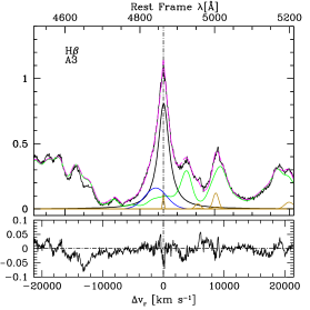
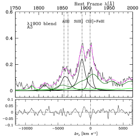
Figure 2: Broad emission line fits of the H$\beta$ spectral region (left) and Aliii$\lambda$1860 for median spectra of two A3 samples, shown after continuum subtraction. Abscissa is rest-frame wavelength; ordinate is normalized intensity. The dashed magenta line shows the model spectrum. The lower panel shows the difference between the observed and the model spectra. The lemon green lines trace Feii  and the dark green one Feiii emission in correspondence of the 1900 blend. The H$\beta$ broad profile (thick line) is isolated after Feii  and narrow line subtraction. Only a faint H$\beta$ narrow component is detected (golden line). The blue line shows the blueshifted residual associated to a non-virial H$\beta$ component. In the right panel, the thick black lines on the right panel trace the Siii$\lambda$1814, Aliii$\lambda$1860, Siiii]$\lambda$1892, and Ciii]$\lambda$1909 in order of increasing wavelength. Note that the Aliii$\lambda$1860 profile is modelled as a doublet with intensity ratio 1858/1863 = 1.2:1.

The left panel of Figure 2 shows profile model fitting to the median bin A3 spectrum (sample of Marziani et al., 2013a). The $R_{\rm FeII}$ value is consistent with the one of I Zw 1 reported in Negrete et al. (2012). Details of model fitting procedures can be found in §  2.4 and Marziani et al. (2010).

2.2 Selecting High $z$ Samples of Eddington Candles

Without IR spectra we lose the $R_{\rm FeII}$ selector employed at $z<$1.0. We must take advantage of quasar abundant rest-frame UV spectra. The first choice would be to use measures of Civ$\lambda$1549 shift, asymmetry and equivalent width because extreme sources tend to show low EW Civ$\lambda$1549 profiles that are blueshifted and blue asymmetric. A measure of Civ$\lambda$1549 shift was chosen as a 4DE1 parameter because it is the best measure of extreme Civ$\lambda$1549 properties. At low $z$ we rely on satellite observations where the HST archive provides the highest S/N and resolution UV spectra for our low $z$ candidates. Data exist in the HST archive for about 130 low $z$ sources of which $n$ = 11 are bin A3 – A4 sources ($R_{\rm FeII}$$>$1.0). Ten of the eleven Feii extreme sources show a significant Civ$\lambda$1549 blueshift confirming its utility as an extreme Eddington selector (Sulentic et al., 2007). The majority of Pop. A sources with $R_{\rm FeII}$$<$1.0 and Pop. B sources show a smaller blueshift and in many cases zero shift or a redshift ($n$ = 3 with shift $>$ 10³ km s^-1).

However, we do not know the geometry of the outflows implied by the profile blueshift. We may miss a considerable number of candidates where orientation diminishes the blueshift. There is also the issue of whether Civ$\lambda$1549 blueshifts are quasi-ubiquitous in high $z$ quasars (Richards et al., 2011). If Civ$\lambda$1549 blueshifts are more common at high $z$ then they may not be useful as a clearcut selector. A further problem is that a selector involving a line shift requires a more accurate estimate of the quasar rest frame which is often missing in high redshift sources.

We propose an alternative high $z$ selector involving the 1900 emission line blend of Aliii$\lambda$1860, Siiii]$\lambda$1892 and Ciii]$\lambda$1909. The blend involving these lines constrains the physical conditions in the broad line emitting gas much the same way as measures of very strong optical Feii. The definition of this selector comes from three sources: 1) measures from a composite spectrum of HST archival data for 10 bin A3 sources (right panel of Fig. 2, Bachev et al., 2004), 2) line ratio measures for I Zw 1 (our bin A3 prototype) from a high S/N and resolution HST spectrum (Laor et al., 1997; Negrete et al., 2012) and 3) measures of SDSS1201+0116 (a high $z$ bin A4 analogue of I Zw 1 from a high S/N VLT spectrum Negrete et al. 2012).

Bachev et al. (2004) noted that the Siiii]$\lambda$1892/Ciii]$\lambda$1909 intensity ratio decreased monotonically along the 4DE1 sequence by a factor $\approx$4 from bin A3 ($\approx$0.8) to bin B1+ ($\approx$0.2). This implies a selection constraint for extreme sources Siiii]$\lambda$1892/Ciii]$\lambda$1909 $>$0.6-0.7. Measures using very high S/N spectra and on the 1900 blend of the A3 composite spectrum (Fig. 2) yield a selection criterion based on two related ratios:

1. Aliii$\lambda$1860/Siiii]$\lambda$1892/ $\geq$ 0.5 and

2. Siiii]$\lambda$1892/Ciii]$\lambda$1909 $\geq$1.0.

Both our low and high redshift selectors are based on more than empiricism because they effectively constrain the range of physical conditions in the line emitting region of the extreme quasars (Baldwin et al., 1996, 2004; Marziani et al., 2010; Negrete et al., 2012). The extreme Feii emission from these sources has been discussed in terms of the densest broad line emitting region ($n_{\mathrm{H}}$$\sim$10¹² cm^-3; Negrete et al. 2012) and extreme metallicity again plausibly connected with high accretion rates.

2.3 Identification of Preliminary Samples

Equipped with low and high redshift selection criteria we identify three samples of extreme Eddington sources over the range $z=$ 0.4 – 3.0.

1. Sample 1: 58 sources with H$\beta$ spectral coverage from an SDSS DR8 sample of 680 quasars in the range $z\approx 0.4-0.75$  (Marziani et al., 2013b). Their spectral bins are A3 and A4. Table 1 lists the 30 and 13 sources in bin A3 and A4 with S/N $\geq$ 15 at 5100 Å. Formats for Tables 1 and 2 are: ID, redshift, restframe flux $\lambda$f_λ, S/N of spectrum, FWHM of virial estimator used, FWHM uncertainty and sample ID. FWHM uncertainties for sample 1 H$\beta$ profiles were assumed to be 10%.

2. Sample 2: 7 sources from a sample of 52 Hamburg-ESO quasars (Marziani et al., 2009) in the range $z$ = 1.0 – 2.5 (all but two $1\lower 2.15277pt\hbox{$\;\buildrel<\over{\sim}\;$}z\lower 2.15277pt\hbox{$\;\buildrel<\over{\sim}\;$}1.6$) with high S/N (VLT-ISAAC) spectra of the H$\beta$ region. They all satisfy the criterion $R_{\rm FeII}$$\geq$ 1.0 within observational uncertainty; 3 of them are however borderline sources with $R_{\rm FeII}$$\approx$ 1.0. The ISAAC sources are meant to cover a redshift range where H$\beta$ observations are very sparse.

3. Sample 3: 63 SDSS sources (additional candidates were identified but require higher S/N data) are listed in Table 2. We extracted spectra for $\approx$3000 sources from SDSS DR6 with coverage of the 1900 blend ($2.0\lower 2.15277pt\hbox{$\;\buildrel<\over{\sim}\;$}z\ \lower 2.15277pt\hbox{$\;\buildrel<\over{\sim}\;$}$ 2.6). Selected sources show emission line ratios Aliii$\lambda$1860/ Siiii]$\lambda$1892 and Ciii]$\lambda$1909/Siiii]$\lambda$1892  satisfying our criterion. A further restriction was imposed by excluding sources with low S/N ($<$ 15) spectra that might have biased FWHM measures as clearly shown by Shen et al. (2008). This yielded a subsample 3 of 42 sources with S/N$\geq$ 15 on the continuum at 1800 Å. FWHM uncertainties were estimated from simulated spectra as a function of Aliii$\lambda$1860 EW, FWHM and S/N.

Sample 1 and 2 are based on flux limited samples analysed in the studies cited above. Sample 3 has no pretence of completeness: the lower fraction of identified xA sources is due to the low S/N of most spectra.

2.4 Emission Line Measurements

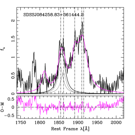
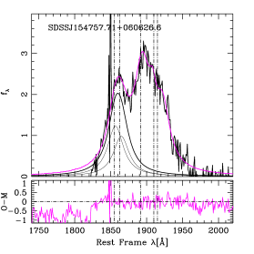
Figure 3: Example of broad emission line fits of the $\lambda$1900 Å blend, shown after continuum subtraction. Abscissa is rest-frame wavelength; ordinate is specific flux in units of 10^-15ergs s^-1 cm^-2 Å^-1. The FWHM of the individual components of the Aliii$\lambda$1860 doublet (thin lines) provide a virial broadening estimator. Total Aliii$\lambda$1860 emission (thick line) can be modeled since the doublet is well-separated from Siiii]$\lambda$1892 and the rest of the blend. The magenta dashed line shows the full model of the $\lambda$1900 Å blend which includes Siiii]$\lambda$1892, and Ciii]$\lambda$1909 and Feiii emission.

Line ratios yield 4DE1 bin assignments. In the optical, $R_{\rm FeII}$ is retrieved from the intensity of the Lorentzian profile representing H$\beta$ and from Fe ii_opt flux in the integrated over the wavelength range 4434 – 4684 Å (Boroson & Green, 1992; Marziani et al., 2003b). In the UV, it is especially the Aliii$\lambda$1860/Siiii]$\lambda$1892 ratio that, with or without Civ$\lambda$1549 measures, provides a selector for high $z$ extreme sources. Figure 3 shows model fits to the 1900 blends for two high $z$ extreme source candidates.

Measurements were made using a nonlinear multicomponent fitting routine that seeks $\chi^{2}$ minimisation between observed and model spectra, i.e., specfit incorporated into iraf (Kriss, 1994). The procedure allows for simultaneous fit of continuum, blended iron emission, and all narrow and broad lines identified in the spectral range under scrutiny. Singly and doubly ionised iron emission (the latter present only in the UV) were modelled with the template method. For the optical Feii emission, we considered the semi-empirical template used by Marziani et al. (2009). This template was obtained from a high resolution spectrum of I Zw 1, with a model of Feii emission computed by a photoionization code in the wavelength range underlying H$\beta$. For the UV Feii and Feiii emission, we considered templates provided by Brühweiler & Verner (2008) and Vestergaard & Wilkes (2001), respectively. The fitting routine scaled and broadened the original templates to reproduce the observed emission. Broad H$\beta$ and the 1900 Å blend lines were fit assuming a Lorentzian function. This assumption follows from analysis of large samples of Pop. A sources (Véron-Cetty et al., 2001; Marziani et al., 2003c; Zamfir et al., 2010; Marziani et al., 2013a): Negrete et al. (2013) verified that H$\beta$, Aliii$\lambda$1860 and Siiii]$\lambda$1892 can be fit with a Lorentzian function whose width is the same for the three lines in Pop. A sources studied with reverberation mapping. The broad H$\beta$ line profile is often asymmetric toward the blue. The line profile has been modeled adding to the Lorentzian component an additional, shifted line component associated to outflows (c.f., Marziani et al., 2013a). Narrow lines ([Oiii]$\lambda\lambda$4959,5007 and H$\beta_{\rm NC}$) were fit with Gaussian functions.

The uncertainty associated with FWHMH$\beta$ was 10% for sample 1, and as reported in Marziani et al. (2009) for the sample 2 (usually $\la$10%). For the UV virial estimator i.e., in cases of lower S/N , synthetic blend profiles were computed as a function of S/N, equivalent width, and individual line width for typical values in our sample (e.g., S/N = 14,22; W(Aliii$\lambda$1860) = 5,10 Å; FWHM = 3000,4000 km s^-1). Statistical measurement errors on each source FWHM were assigned to the value computed for the synthetic case with closest lower S/N, closest lower equivalent width and closest FWHM.

2.5 Consistency of criteria

If optical and UV rest frame range are both covered, it becomes possible to test that the condition $R_{\rm FeII}$$\ga$ 1 is fully interchangeable with Aliii$\lambda$1860/Siiii]$\lambda$1892$\ga 0.5$ and Siiii]$\lambda$1892/ Ciii]$\lambda$1909 $\ga 1$ (i.e., $R_{\rm FeII}$$\ga$ 1 $\Leftrightarrow$ Aliii$\lambda$1860/ Siiii]$\lambda$1892$\ga 0.5$ and Siiii]$\lambda$1892/ Ciii]$\lambda$1909 $\ga 1$). If only xA sources are considered, at low $z$ not many spectra covering the 1900 blend are available in the MAST archive. At high $z$, few objects have H$\beta$ covered in IR windows with adequate resolution spectroscopy. At present, data available to us encompass 6 low-$z$ (including I Zw 1, and excluding all RL sources) and 3 HE sources of sample 2.

Low-$z$ –

We measured with specfit both UV ratios on $\approx$ 100 sources of Bachev et al. (2004) for which the 1900 blend is covered from HST/FOS observations, as a test of consistency for the two criteria. Among them, six A3 sources (1H 0707–495, HE 0132–4313, I Zw 1, PG 1259+593, PG1415+451, PG1444+407) are included. Spectral type assignments and references to the used data can be retrieved from Sulentic et al. (2007).

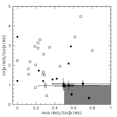
Figure 4: The distribution of Pop. A sources (A1: open squares; A2: filled squares; A3: filled circles) in the plane defined by the ratios Ciii]$\lambda$1909/Siiii]$\lambda$1892 and Aliii$\lambda$1860/Siiii]$\lambda$1892. The area associated with xA sources is the lower-left shaded box. Error bars are shown for borderline sources only. The source with a lower limit to Aliii$\lambda$1860/Siiii]$\lambda$1892 is PG 1415+415, whose Aliii$\lambda$1860 profile is affected by absorption lines.

All Pop. B (56) sources save one show Ciii]$\lambda$1909/Siiii]$\lambda$1892 $\ga$2.0 and are therefore immediately excluded by the selection criteria; many sources appear dominated by Ciii]$\lambda$1909 emission, with Ciii]$\lambda$1909/ Siiii]$\lambda$1892 $\gg$1. Fig. 4 shows the distribution of 37 Pop. A sources in the plane Ciii]$\lambda$1909/Siiii]$\lambda$1892 vs Aliii$\lambda$1860/Siiii]$\lambda$1892, with special attention to sources that are “borderline” and for which error bars are also shown. All type A3 objects fall at the border or within the shaded region defined by the conditions Aliii$\lambda$1860/Siii$\lambda$1814$\geq$0.5 and Ciii]$\lambda$1909/Siiii]$\lambda$1892 $\leq$1. Sources falling close to the border show $R_{\rm FeII}$ $\approx 1$, while the two sources with $R_{\rm FeII}$$>1$ are well within the region. The only source (Mark 478) that is not formally of spectral type A3 and falls close to the area Aliii$\lambda$1860/Siii$\lambda$1814$\geq$0.5 Ciii]$\lambda$1909/Siiii]$\lambda$1892 $\leq$1 is of type A2 with $R_{\rm FeII}$$\approx$0.92. Fig. 4 confirms the consistency of the optical and UV criteria: no source of $R_{\rm FeII}$$<$ 0.9 falls in the domain Ciii]$\lambda$1909/ Siiii]$\lambda$1892$\la$1 and Aliii$\lambda$1860/Siiii]$\lambda$1892/ $\geq$ 0.5, and no source with $R_{\rm FeII}$$\ga$0.9 falls, within the error, outside of it.

High-$z$ –

Three sources of sample 2 have newly-obtained observations covering the Civ$\lambda$1549– Ciii]$\lambda$1909 emission lines (Martínez-Carballo et al. 2014, in preparation): HE0122–3759 ($\log L\approx 47.7$ [ergs s^-1]), HE0358–3959 ($\log L\approx 47.3$), HE1347– 2457 ($\log L\approx 47.9$). In all cases, the condition on the UV lines is satisfied.

The prototype source I Zw1 has $\log L\approx 45.6$ [ergs s^-1]; the lowest luminosity and nearest source is 1H 0707–495 with $\log L\approx 45.04$ at $z\approx 0.04$; the luminosity of the three PG sources is the range $\log L\approx 45.5-47.0$. The condition $R_{\rm FeII}$$\geq$ 1 implied Aliii$\lambda$1860/Siiii]$\lambda$1892 $\geq 0.5$ in all cases, and all individual spectra consistently showed the features typical of A3 sources (low Civ$\lambda$1549 equivalent width, large Civ$\lambda$1549 blueshift, etc.). Within the limit of the available data, the optical and UV criteria are consistent over a very large range in luminosity and redshift, $45\la\log L\la 48$, $0.04\la z\la 3$.

2.6 The a-posteriori distribution of Eddington ratios

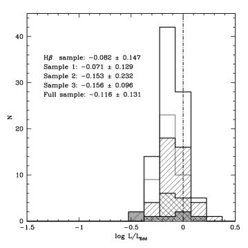
Figure 5: Distribution of $\log$$L/L_{\rm Edd}$ for the sources of the full sample considered in this paper. The shaded histograms shows the distribution of $L/L_{\rm Edd}$ for subsamples 1 and 2 (dark shaded) based on H$\beta$, and sample 3 based on the 1900 blend (thick grey line). The cross-hatched histogram represents the distribution of the A4^m sources in sample 1 (sample 1a of Tab. 1).

An estimate of the spread associated to the $L/L_{\rm Edd}$ distribution comes from the a-posteriori analysis of our sample. We computed $M_{\rm BH}$  following Assef et al. (2011) and applied the bolometric correction indicated by Richards et al. (2006) (optical) and derived using the Mathews & Ferland (1987) continuum (UV, see discussion on $B.C.$ later in this section). The resulting $L/L_{\rm Edd}$ distribution is shown in Fig. 5. The dispersion in the full sample is $\sigma\approx 0.13$. This is consistent with current search techniques that allow us to identify sources radiating within $\pm$0.15 dex in log $L/L_{\rm Edd}$ (Steinhardt & Elvis, 2010). Inter-subsample systematic differences are smaller than the full sample dispersion. A4 H$\beta$ sources of of sample 1 (sample 1a in Tab. 1; cross-hatched histogram in Fig. 5) do not differ significantly from A3 sources. There is a systematic difference between the H$\beta$ and Aliii$\lambda$1860 sample, by $\Delta\log\lambda_{\mathrm{Edd}}\approx 0.07<1\sigma$  that is dependent on the assumed ratio of the $B.C.$ at 1800 Å and 5100 Å ($\approx$ 0.63). This can give to an important systematic effect discussed in §6.2.

Armed with selection criteria to isolate sources clustering around $L/L_{\rm Edd}$$\approx 1$ and having defined preliminary samples, we now discuss how we can derive luminosity information without prior redshift knowledge.

3 Measuring luminosity from emission line properties

The bolometric luminosity – black hole mass ratio of a source radiating at Eddington ratio $\lambda_{\mathrm{Edd}}$ can be expressed as:

$$\frac{L}{M}\approx 10^{4.53}\lambda_{\mathrm{Edd}}\left(\frac{L}{M_{\rm BH}}\right)_{\odot}\approx 10^{4.81}\lambda_{\mathrm{Edd}}~{}\mathrm{erg~{}s}^{-1}~{}{\mathrm{g}}^{-1},$$ (1)

where $M_{\rm BH}$ is the black hole mass, and $L$ the bolometric luminosity. Under the assumption of virial motion the bolometric luminosity is (setting $\xi\approx 10^{4.81}$ erg s^-1 g^-1):

$$L\approx\xi\lambda_{\mathrm{Edd}}M\approx\xi\lambda_{\mathrm{Edd}}f_{\mathrm{S}}\frac{r_{\mathrm{BLR}}(\delta v)^{2}}{G}.$$ (2)

where $f_{\mathrm{S}}$ is the structure factor (Collin et al., 2006), $\delta v$ a virial velocity dispersion estimator, $G$ is the gravitational constant, and $r_{\mathrm{BLR}}$ the BLR radius. The ionization parameter can be written as (under the assumption – satisfied by spherical symmetry – that the line emitting gas is seeing the same continuum that we observe):

$$U=\frac{\int_{\nu_{0}}^{+\infty}\frac{L_{\nu}}{h\nu}d\nu}{4\pi n_{\mathrm{H}}cr_{\mathrm{BLR}}^{2}}$$ (3)

where $L_{\nu}$ is the specific luminosity per unit frequency, $h$ is the Planck constant, $\nu_{0}$ the Rydberg frequency, $c$ the speed of light, and $n_{\mathrm{H}}$ the hydrogen number density. The parameter $r_{\mathrm{BLR}}$ can be interpreted as the distance between the central source of ionizing radiation and the part of the line emitting region that responds to continuum changes. Values of $r_{\mathrm{BLR}}$  from reverberation mapping (Peterson et al., 1998) of H$\beta$ are available for $\approx$60 low-$z$ Seyfert 1 galaxies and quasars (Bentz et al., 2009, 2013). The most recent $r_{\mathrm{BLR}}$ determinations show a correlation with luminosity $r_{\mathrm{BLR}}\propto L^{0.533^{+0.035}_{-0.033}}$ (Bentz et al., 2013), consistent with $U$ remaining constant with luminosity.

There is an alternative way to derive $r_{\mathrm{BLR}}$ if one has a good estimate of the product of $n_{\mathrm{H}}$  $\times$$U$. Without loss of generality,

$$r_{\mathrm{BLR}}=\left[\frac{\int_{\nu_{0}}^{+\infty}\frac{L_{\nu}}{h\nu}d\nu}{4\pi Un_{\mathrm{H}}c}\right]^{1/2}=\left(\frac{{\kappa L}}{4\pi Un_{\rm H}ch\bar{\nu_{\mathrm{i}}}}\right)^{1/2}$$ (4)

where the ionizing luminosity is assumed to be $L_{\mathrm{ion}}=\kappa L$, with $\kappa\approx 0.5$. The number of ionizing photons is $\kappa L/h\bar{\nu_{\mathrm{i}}}$, where $\bar{\nu_{\mathrm{i}}}$ is the average frequency of the ionizing photons. Several workers in the past used Eq. 4 to estimate $r_{\mathrm{BLR}}$ (Padovani et al., 1990; Wandel et al., 1999; Negrete, 2011). Analysis of a subsample of reverberation mapped sources indicates that Eq. 4 provides estimates of $r_{\mathrm{BLR}}$ not significantly different from reverberation values (Negrete et al., 2013). Bochkarev & Gaskell (2009) also show that a photoionization analysis based on the H$\beta$ luminosity provides $r_{\mathrm{BLR}}$  estimates consistent with reverberation mapping.

Inserting Eq. 4 into Eq. 2:

$$L \approx \frac{\xi}{\sqrt{4\pi ch}G}\frac{\lambda_{\mathrm{Edd}}f_{\mathrm{S}}\kappa^{\frac{1}{2}}}{\bar{\nu_{\mathrm{i}}}^{\frac{1}{2}}}\frac{L^{\frac{1}{2}}}{(n_{\mathrm{H}}U)^{\frac{1}{2}}}(\delta v)^{2}$$

$$\approx \frac{\xi^{2}}{4\pi chG^{2}}\frac{\lambda_{\mathrm{Edd}}^{2}f_{\mathrm{S}}^{2}\kappa}{\bar{\nu_{\mathrm{i}}}}\frac{1}{(n_{\mathrm{H}}U)}(\delta v)^{4}$$

Then:

$$L\approx 7.8~{}10^{44}\frac{\lambda_{\mathrm{Edd,1}}^{2}\kappa_{0.5}f^{2}_{\mathrm{S,2}}}{h{\bar{\nu}_{\mathrm{i}},_{\mathrm{100\,eV}}}}\frac{1}{(n_{\mathrm{H}}U)_{10^{9.6}}}(\delta v)_{1000}^{4}~{}~{}\mathrm{erg~{}s^{-1}}$$ (6)

where the energy value has been normalized to 100 eV ($\bar{\nu_{\mathrm{i}}}\approx 2.42\,10^{16}$ Hz), the product $(n_{\mathrm{H}}U)$ to the “typical” value $10^{9.6}$ cm^-3 (Padovani & Rafanelli, 1988; Matsuoka et al., 2008; Negrete et al., 2012) and $\delta v$ to 1000 km s^-1.

Eq. 6 (hereafter the “virial” luminosity equation) is formally valid for any $L/L_{\rm Edd}$; the key issue in the practical use of Eq. 6 is to have a sample of sources tightly clustering around an average $L/L_{\rm Edd}$ (whose value does not need to be 1, or to be accurately known). At present, we can identify sources with $\lambda_{\mathrm{Edd}}\rightarrow 1$, but it is still possible that an eventual analysis may employ different spectral types representative of much different $L/L_{\rm Edd}$ average values. In practice, an approach followed in this paper has been to consider Eq. 6 in the form $L\approx\mathcal{L}_{0}\delta v^{4}$, where $\mathcal{L}_{0}$ has been set by the best guess of the quasar parameters with $\lambda_{\mathrm{Edd}}\rightarrow 1$. This will imply a value of $H_{0}$, and to ignore source-by-source diversity. A second possibility is to compute $L\approx\mathcal{L}_{0}$ to yield the concordance value of $H_{0}$, especially for a sample of sources at very low-$z$  ($\lower 2.15277pt\hbox{$\;\buildrel<\over{\sim}\;$}0.05$) where $\Omega_{\mathrm{M}}$ and $\Omega_{\Lambda}$ are insignificant in luminosity computations. Statistical and systematic errors will be discussed in §6.

4 Preliminary Results

4.1 Comparison of virial luminosity and luminosity derived from redshift

Using our three combined samples we initially consider four cases: (1) “concordance cosmology” ($\Omega_{\mathrm{M}}$+ $\Omega_{\Lambda}$= 1.0, $\Omega_{\mathrm{M}}$= 0.28, $\Omega_{\mathrm{k}}$= 0.0), (2) an “empirical” open model ($\Omega_{\mathrm{M}}$= 0.1, $\Omega_{\Lambda}$= 0.0, $\Omega_{\mathrm{k}}$=0.0), (3) a matter-dominated Universe ($\Omega_{\mathrm{M}}$= 1.00, $\Omega_{\Lambda}$= 0.0, $\Omega_{\mathrm{k}}$=0.0) and (4) a $\Lambda$-dominated model $\Omega_{\mathrm{M}}$= 0.0, $\Omega_{\Lambda}$= 1.0, $\Omega_{\mathrm{k}}$=0.0). Expected bolometric luminosity differences as a function of redshift with respect to an empty Universe are shown in Figure 6.

The transverse comoving distance can be written as

$$d_{\mathrm{p}}=\frac{c}{H_{0}}f(z,\Omega_{\Lambda},\Omega_{\mathrm{M}}),$$ (7)

where $f(z,\Omega_{\Lambda},\Omega_{\mathrm{M}})$ is a function of $z$ with $\Omega_{\Lambda}$ and $\Omega_{\mathrm{M}}$ assumed as parameters reported in Perlmutter et al. (1997). Bolometric luminosity is defined by the relation:

$$\log L=\log\left[4\pi\lambda f_{\lambda}d_{\mathrm{p}}^{2}(H_{0},z,\Omega_{\mathrm{M}},\Omega_{\Lambda})\right]+B.C.,$$ (8)

where $B.C.$ is the bolometric correction and $f_{\lambda}$ the rest frame specific flux at 5100 Å or 1800 Å. Assumed bolometric corrections are: $B.C.$ = 1.00 for $\lambda f_{\lambda}$ measured at 5100 Å  (Richards et al., 2006), and $B.C.$ = 0.800 when $\lambda f_{\lambda}$ was measured at 1800 Å. These bolometric correction are computed for the Mathews & Ferland (1987) continuum that is believed appropriate for Pop. A quasars.

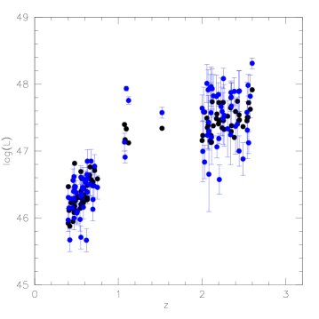
Figure 7: Bolometric luminosity (in logarithmic scale) for our sample of 92 quasars, computed from Eq. 6 (blue circles) and from the customary relationship using concordance cosmology (assuming $H_{0}$ = 70 km s^-1Mpc^-1). The bottom panel shows the residuals. The line is an (unweighted) linear least-square (lsq) fit to the residuals.

We compare two sets of luminosity values as a function of redshift: one derived from the redshift $L$ (Eq. 8) and the other from the virial luminosity (Eq. 6). We assume ${\cal L}_{0}\approx 1.16\cdot 10^{45}$ ergs s^-1 from the best guess of parameters entering Eq. 6, for the standard continuum of Mathews & Ferland (1987): $\kappa\approx 0.6$, $n_{\mathrm{H}}$$U$ $\approx 10^{9.6}$ cm^-3, $h\bar{\nu_{\mathrm{i}}}\approx 41$ eV, and $f_{\mathrm{S}}\approx 1.5$ as recommended by Collin et al. (2006). Figure 7 shows data points computed from the virial equation (blue circles) and values computed from the redshift in the case of concordance cosmology ($H_{0}$=70 km s^-1 Mpc^-1, $\Omega_{\mathrm{M}}$=0.28, $\Omega_{\Lambda}$=0.72). Error bars are 1$\sigma$ uncertainties from FWHM uncertainty estimates given in §2 and are reported in Tab. 1 and 2 (Fig. 7). Residuals defined as $\Delta=\log L(v)-\log L$ are shown in the bottom panel.

The average of residuals ($\bar{\Delta}$) is nonzero and there is a slightly nonzero slope $b\approx+0.03$ in the lower panel of Fig. 7, not significantly different from 0 since its 1$\sigma$ error is $\sigma_{\mathrm{b}}\approx$0.075. The shape of the residuals depends on redshift, as it is related to the shape of $f(z,\Omega_{\mathrm{M}},\Omega_{\Lambda})$ and hence to the metric and the $\Omega$s:

$$\Delta(z,H_{0},\Omega_{\mathrm{M}},\Omega_{\Lambda}) = \log L(v)-[\log(4\pi c^{2})+\log(H_{0}^{2})$$ (9)

$$+\log(\lambda f_{\lambda})+\,B.C.+\log f^{2}(z,\Omega_{\mathrm{M}},\Omega_{\Lambda})]$$

$$= const.-\log(H_{0}^{2})-\log f^{2}(z,\Omega_{\mathrm{M}},\Omega_{\Lambda})$$

The above equation shows that $H_{0}$ sets the scale for $\Delta\log L$ in a way that is not dependent on redshift. A change in the model involving different $\Omega$ values leaves correlated residuals:

$$\Delta(z,H_{0},\Omega_{\mathrm{M}},\Omega_{\Lambda})=\bar{\Delta}(H_{0},\Omega_{\mathrm{M}},\Omega_{\Lambda})+\zeta(z,\Omega_{\mathrm{M}},\Omega_{\Lambda}).$$ (10)

$\bar{\Delta}$ is not formally dependent on $z$ since it is defined as an average, and its value is fixed once the redshift distribution of a sample is given. Retrieving $\zeta(z,\Omega_{\mathrm{M}},\Omega_{\Lambda})$ when $\Delta(z,H_{0},\Omega_{\mathrm{M}},\Omega_{\Lambda})\equiv 0$ is equivalent to finding $\Omega_{\mathrm{M}}$ and $\Omega_{\Lambda}$ and hence the appropriate model. More explicitly, the difference $\zeta(z,\Omega_{\mathrm{M}},\Omega_{\Lambda})$ between a cosmology independent luminosity estimator (the virial luminosity) and a luminosity computed from luminosity distance should become identically zero as a function of redshift for the correct cosmological model.

We consider the conventional $\chi^{2}$ computed from the squared $\Delta$s as a goodness of fit estimator. In principle the residuals $\Delta(z,H_{0},\Omega_{\mathrm{M}},\Omega_{\Lambda})$ could be fit with an analytical approximation of $\zeta(z,\Omega_{\mathrm{M}},\Omega_{\Lambda})$ as complex as needed. Our preliminary data allow only a simple linear least square fit to the residuals: $\Delta(z)=a+b\cdot z$. The sought-for model requires $a=b=0$. In the following analysis we found expedient to consider the normalized average $\bar{\Delta}/\sigma_{\bar{\Delta}}$  and the normalized slope $b/\sigma_{\mathrm{b}}$. $\bar{\Delta}/\sigma_{\bar{\Delta}}$ and $b/\sigma_{\mathrm{b}}$ are both $t$-distributed estimators that for our sample size can be considered normally distributed. They both provide statistical confidence limits $\propto 1/({\mathrm{rms}}/\sqrt{N-1})$, where $N=92$. The normalized average and the slope estimator have been computed under the assumption that the rms scatter of our data is an estimate of uncertainty for individual measures (Press et al., 1992, Ch. 15). The slope estimator is not a very tightly constraining parameter; however it has the considerable advantage to be fully independent on $H_{0}$, and to provide a straightforward representation of the systematic trends associated with $\Omega_{\mathrm{M}}$ and $\Omega_{\Lambda}$ as function of $z$.

The rms value ($\approx 0.365$) is intrinsic to our dataset and will probably not change much with larger samples unless FWHM measures with substantially higher accuracy, and a reduction of other sources of statistical errors, are obtained (§6). Given the redshift range of our data, a change in $\Omega_{\mathrm{M}}$ gives rise to a change in slope of the residuals $\Delta(z)$ that strongly affects $\bar{\Delta}$ (as can be glimpsed from Fig. 6).

4.2 Selected alternative cosmologies

Table 3 reports normalized average $\bar{\Delta}/\sigma_{\bar{\Delta}}$, $b$, and $\chi^{2}$ values for the selected cosmological models of Fig. 6, assuming fixed $H_{0}$= 70 km s^-1 Mpc^-1. Normalized $\chi^{2}/\chi^{2}_{\mathrm{min}}$ values of 1.1, 1.41, and 1.79 limit acceptable fits at confidence levels of 1$\sigma$, $2\sigma$, and $3\sigma$ respectively. Note that $\chi^{2}$ and $\bar{\Delta}/\sigma_{\bar{\Delta}}$ values are affected by $H_{0}$, while $b$ is not dependent on $H_{0}$.

Extreme implausible cases such as a matter ($\Omega_{\mathrm{M}}$=1) or $\Lambda$-dominated ($\Omega_{\Lambda}$=1) Universe are ruled out. The case with $\Omega_{\mathrm{M}}$= 1 ($\Omega_{\Lambda}$= 1) will yield a large positive (negative) slope meaning that redshift based estimates are underluminous (over luminous) with respect to virial luminosities. The concordance case is favored by our dataset, with $\chi^{2}\approx 1.05$ (Fig. 7). The “empirical” model with $\Lambda=0$ and $\Omega_{\mathrm{M}}$= 0.1 is not disfavored by our data, with $\chi^{2}\approx 1.08$ if $H_{0}$= 70 km s^-1 Mpc^-1. The two cases, concordance and “empirical” $\Omega_{\mathrm{M}}$= 0.1 (along with the unrealistic case of a fully empty Universe) cannot be statistically distinguished since their slopes $b$ are close to 0 and $|b/\sigma_{\mathrm{b}}|\la 1$.

Obtaining a solution close to the one of concordance cosmology is not a consequence of how the parameters entering Eq. 6 were obtained. Parameters related to continuum shape and ionising photon flux were not derived assuming any particular luminosity. The assumed value of ${\cal L}_{0}$ depends from $H_{0}$ since the assumed $L/L_{\rm Edd}$  depends on $H_{0}$. However, effects of $\Omega_{\mathrm{M}}$ and $\Omega_{\Lambda}$ are negligible since $L/L_{\rm Edd}$ was calibrated on a very low-$z$ source, I Zw 1 (Fig. 6).

4.3 $H_{0}$, $\Omega_{\mathrm{M}}$ and $\Omega_{\Lambda}$ in a flat Universe

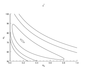
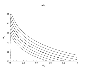
Figure 8: Top: Normalized $\chi^{2}$ of luminosity residuals computed between virial estimates and models, for a flat geometry ($\Omega_{\mathrm{M}}+\Omega_{\Lambda}=1.00$) as a function of $H_{0}$ and $\Omega_{\mathrm{M}}$. Middle: same for average of residuals normalized to standard deviation. One contour line brackets the most likely value and the other three trace the uncertainties at 1$\sigma$, 2$\sigma$ and $3\sigma$ confidence levels. Bottom: Behavior of normalized slope parameter $b/\sigma_{\mathrm{b}}$ as a function of $\Omega_{\mathrm{M}}$. The lower –2, –1$\sigma$ and $+1,+2\sigma$ limits are shown by dotted lines.

Assuming a flat geometry ($\Omega_{\mathrm{M}}$+ $\Omega_{\Lambda}$= 1, $\Omega_{\mathrm{k}}$= 0) the normalized average is influenced by changes in $H_{0}$ and $\Omega_{\mathrm{M}}$ ($\Omega_{\Lambda}$ is set by $\Omega_{\mathrm{M}}$). Fig. 8 shows $\chi^{2}$  (top), $\bar{\Delta}/\sigma_{\bar{\Delta}}$ (middle) as a function of $H_{0}$ and $\Omega_{\mathrm{M}}$, and $|b/\sigma_{\mathrm{b}}|$ as a function of $\Omega_{\mathrm{M}}$. The $\chi^{2}$  contour lines trace 4 values of the ratio $\chi^{2}/\chi^{2}_{\mathrm{min}}$: $\chi^{2}\approx\chi^{2}_{\mathrm{min}}$, and 3 values meant to represent the 0.32, 0.05, and 0.003 probability interval considering that the probability of the $\chi^{2}/\chi^{2}_{\mathrm{min}}$ ratio follows an F-distribution (Bevington, 1969). The $\chi^{2}$ diagram indicate that $\Omega_{\mathrm{M}}$ is constrained within 0.05 and 0.8 if $H_{0}$ is not chosen a priori. The lines in the $\bar{\Delta}/\sigma_{\bar{\Delta}}$  plot (middle panel of Fig. 8) identify a curved strip close to 0, and values 1, 2, 3. The lines of value 1,2,3 trace the corresponding 1,2,3 $\sigma$ confidence levels. The bottom panel of Fig. 8 shows the behaviour of $|b/\sigma_{\mathrm{b}}|$ as a function of $\Omega_{\mathrm{M}}$. The minimum identifies the condition $b=0$. Changing $\Omega_{\mathrm{M}}$ will increase the slope that will become significantly different from 0 at 1 and 2 $\sigma$ confidence levels when $|b/\sigma_{\mathrm{b}}|$ =1 and 2. It is possible to define only –2, –1, and $+1$, $+2\sigma$ uncertainties: $\Omega_{\mathrm{M}}$$\approx$ 0.19${}^{+0.16}_{-0.08}$, and $\approx$ 0.19${}^{+0.76}_{-0.15}$ at 1 and $2\sigma$, respectively.

Once an $H_{0}$ value is assumed as indicated by $\chi^{2}_{\mathrm{min}}$ or $b=0$, uncertainties on $\Omega_{\mathrm{M}}$  are significantly reduced if the normalized average is used as a confidence limit estimator. Eq. 6 in the form $L={\cal L}_{0}\delta v^{4}_{1000}$, with ${\cal L}_{0}\approx 1.16\cdot 10^{45}$ ergs s^-1, implies b = 0 and a minimum $\chi^{2}$ at $H_{0}$ $\approx$ 71 km s^-1 Mpc^-1, yielding $\Omega_{\mathrm{M}}$$\approx$ 0.19${}^{+0.07}_{-0.05}$ at 1$\sigma$, and 0.19${}^{+0.21}_{-0.12}$ at 3$\sigma$ (middle panel of Fig. 8). Broader limits are inferred from the normalized $\chi^{2}$ once $H_{0}$ is prefixed because $\chi^{2}$ includes the uncertainty in $H_{0}$ that we may instead assume a priori. Uncertainties from $\chi^{2}$, $|b/\sigma_{\mathrm{b}}|$ and $\bar{\Delta}/\sigma_{\bar{\Delta}}$  reflect statistical errors only. Constraints are already significant although uncertainties are not as low as those derived from the combination of recent surveys (Hinshaw et al., 2012; Planck Collaboration et al., 2013).

4.4 Constraints on $\Omega_{\mathrm{M}}$ and $\Omega_{\Lambda}$

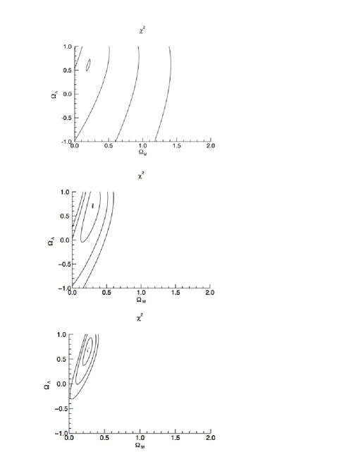
Figure 9: Normalized $\chi^{2}$ behavior in the $\Omega_{\mathrm{M}}$ – $\Omega_{\Lambda}$ plane for data sample presented in this work (top) and mock samples with rms=0.2 (middle) and rms=0.1 (bottom). Contour lines trace $\chi^{2}/\chi^{2}_{\mathrm{min}}$ at confidence limits 1,2,3 $\sigma$.

Rather loose constraints are also obtained where $\Omega_{\mathrm{M}}$ and $\Omega_{\Lambda}$ are left free to vary once $H_{0}$ is assumed ($H_{0}$= 70 km s^-1 Mpc^-1). The top panel of shows the $\chi^{2}$ behavior in the plane $\Omega_{\mathrm{M}}$ and $\Omega_{\Lambda}$. Present data yield $\Omega_{\mathrm{M}}$$\approx$ 0.19${}^{+0.24}_{-0.19}$ and $\Omega_{\mathrm{M}}$$\approx$ 0.19${}^{+1.04}_{-0.19}$ at 1 and 3$\sigma$ confidence level. $\Omega_{\Lambda}$ is unconstrained within the limits of Fig. 9.

5 Prospects for improvement: analysis of synthetic datasets

The limits on $\Omega_{\mathrm{M}}$, and $\Omega_{\Lambda}$ in Fig. 9 are not strong compared to previous studies despite the fact that $\Omega_{\Lambda}$ and $\Omega_{\mathrm{M}}$ are close to currently accepted ones. Our preliminary sample is too small and inhomogeneous. Extreme Eddington sources are estimated to include a sizable minority of the quasar population – most likely $\approx$10%. Significant improvements can come from an increase in sample size with high S/N observations, and by reducing the (large) statistical error in the dataset analyzed here (§6.1).

To quantify the improvement that can be expected from the reduction in statistical errors, synthetic data were created by adding Gaussian deviates to the luminosity computed for the concordance case ($H_{0}$= 70, km s^-1 Mpc^-1, $\Omega_{\mathrm{M}}$$=0.28$, $\Omega_{\Lambda}$$=0.72$), assuming a uniform redshift distribution. In other words, artificial luminosity differences were made to scatter with a Gaussian distribution around the luminosities derived assuming concordance cosmology. This approach is meant to model sources of statistical error that may be present in the virial and $z$-based computations (i.e., FWHM uncertainty, errors in spectrophotometry and bolometric luminosity).

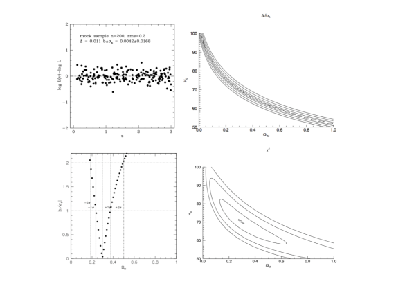
Figure 10: Hypothetical results on mock sample with rms=0.2. The upper left panel shows 200 synthetic data points whose virial luminosity is assumed to deviate (randomly) from the concordance case according to a Gaussian distribution with $\sigma$ = 0.2. Upper right: $\bar{\Delta}/\sigma_{\bar{\Delta}}$ as a function of $H_{0}$ and $\Omega_{\mathrm{M}}$. Bottom left: $|b/\sigma_{\mathrm{b}}|$ as a function of $\Omega_{\mathrm{M}}$. Lower right: normalized $\chi^{2}$ as a function of $H_{0}$ and $\Omega_{\mathrm{M}}$. $\bar{\Delta}/\sigma_{\bar{\Delta}}$, $|b/\sigma_{\mathrm{b}}|$ and $\chi^{2}$ computations assume a a flat geometry ($\Omega_{\mathrm{M}}+\Omega_{\Lambda}=1.00$). See text for more details.

Figure 10 (top left panel) shows the residual as a function of redshift and reports average and dispersion for a mock sample of 200 sources with rms=0.2. The top right, lower left, and lower right panels of Figure 10 show the behaviours of $\chi^{2}$, $|b/\sigma_{\mathrm{b}}|$, and $\bar{\Delta}/\sigma_{\bar{\Delta}}$ respectively, computed assuming $\Omega_{\mathrm{M}}$+$\Omega_{\Lambda}$=1. Meaningful limits can be set in this hypothetical case. The $|b/\sigma_{\mathrm{b}}|$ estimator yields $\Omega_{\mathrm{M}}$$\approx 0.30^{+0.20}_{-0.12}$ at a 2$\sigma$ confidence level, with no assumption on $H_{0}$. If $H_{0}$ = 70 km s^-1 Mpc^-1, $\bar{\Delta}/\sigma_{\bar{\Delta}}$ (top right panel of Fig. 10 ) indicates $\Omega_{\mathrm{M}}$$\approx 0.28^{+0.02}_{-0.02}$ (1 $\sigma$).

The middle panel of Fig. 9, computed for unconstrained $\Omega_{\mathrm{M}}$ + $\Omega_{\Lambda}$, indicates $\Omega_{\mathrm{M}}$$\approx 0.30^{+0.12}_{-0.09}$ at 1$\sigma$ confidence level, with poor constraints on $\Omega_{\Lambda}$. The $\chi^{2}$  distribution for the mock samples was computed as for the real data, varying $\Omega_{\mathrm{M}}$ and $\Omega_{\Lambda}$ with no constraints on their sum.

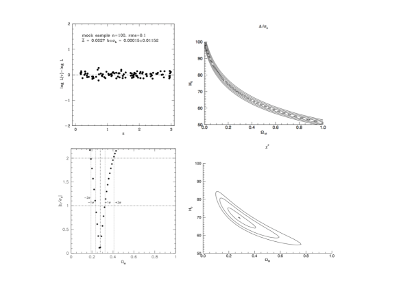
Figure 11: Hypothetical results on mock sample with rms=0.1. Meaning of panels and symbols is the same of previous Figure.

The upper left panel of Fig. 11 (organised as Fig. 10 for the $\Omega_{\mathrm{M}}$+ $\Omega_{\Lambda}$= 1 case) shows a mock sample of 100 sources with rms$\approx$0.1 that is otherwise identical to the previous case. The $|b/\sigma_{\mathrm{b}}|$ estimator yields $\Omega_{\mathrm{M}}$$\approx 0.28^{+0.13}_{-0.09}$ at a 2$\sigma$ confidence level, with no assumption on $H_{0}$. If $H_{0}$ = 70 km s^-1 Mpc^-1, $\bar{\Delta}/\sigma_{\bar{\Delta}}$ (top right panel of Fig. 11) yields $\Omega_{\mathrm{M}}$ with an uncertainty $\pm 0.05$ at a 3$\sigma$ confidence level. From the $\chi^{2}$ distribution (lower right panel of Fig. 11), we derive $\Omega_{\mathrm{M}}$$\approx 0.28^{+0.07}_{-0.06}$, and $\Omega_{\mathrm{M}}$$\approx 0.28^{+0.005}_{-0.015}$ if $H_{0}$ = 70 km s^-1 Mpc^-1 and $\Omega_{\mathrm{M}}$+$\Omega_{\Lambda}$=1. The bottom panel of Fig. 9 ($\Omega_{\mathrm{M}}$+ $\Omega_{\Lambda}$ unconstrained) indicates $\Omega_{\mathrm{M}}$$\approx 0.28^{+0.04}_{-0.08}$ at 1$\sigma$ confidence level, again with poor constraints on $\Omega_{\Lambda}$.

The mock sample improvement over our real sample comes from the larger sample size $N$ (a factor $\sqrt{\frac{N}{92}}$), lower intrinsic rms (a factor 2 – 4), and the uniform distribution in redshift. A reduction of errors associated with the method is therefore tied to an increase in sample size since uncertainties of $\bar{\Delta}$  and $|b/\sigma_{\mathrm{b}}|$ decrease with $1/\sqrt{N}$. Achieving rms$\approx$0.1 would require careful consideration of several systematic effects summarized below, or the definition of a large sample ($\sim$ 1000) of quasars (§6.1).

The value of $\Omega_{\Lambda}$  is affected by larger uncertainty than $\Omega_{\mathrm{M}}$, but significant constraints (for example, the verification that $\Omega_{\Lambda}$$>$0 at a 2$\sigma$ confidence level) are within the reach. The weak constraints on $\Omega_{\Lambda}$ stem from 1) the large errors, 2) the redshift range. Mock sample sources are assumed to spread uniformly over the $z$ range 0.1 – 3.0, but only $z\lower 2.15277pt\hbox{$\;\buildrel<\over{\sim}\;$}1.2$ is strongly affected by $\Omega_{\Lambda}$ (Fig. 6) so that only $\frac{1}{3}$ of the sources are in the relevant range.

We will set more stringent limits on the requirements for an observational program after discussing sources of statistical and systematic uncertainty.

6 Limitations and sources of error/uncertainty

6.1 Statistical error budget

Estimation of the $\Omega$s is affected by statistical errors that will be significantly reduced with larger samples and better source spectra. The residual distribution is affected by errors on the parameters entering into the virial equation (Eq. 6) and into the customary determination of the quasar luminosity from redshift (Eq. 8). In the following each source of statistical error is discussed separately, first for the virial equation and then for the $z$-based $L$ determination. Col. 2 of Table 4 reports the 1$\sigma$ errors as estimated in the following paragraphs, propagating them quadratically to obtain an estimate of statistical error that should be compared with the rms derived from our sample.

6.1.1 Virial equation

Eddington ratio $\lambda_{\mathrm{Edd}}$

– The $L/L_{\rm Edd}$ value of I Zw 1 is consistent with unity (§2), although the exact value depends on the normalization assumed for $M_{\rm BH}$ and on the bolometric correction. The $L/L_{\rm Edd}$ distribution of Fig. 5 shows $\sigma\approx$ 0.13. This dispersion value includes orientation effects. It is unlikely that a larger sample can be obtained with a significantly lower scatter unless scatter is reduced if part of the dispersion can be accounted for by systematic trends (§6.2).

Factor $\kappa/\bar{\nu_{\rm i}}$

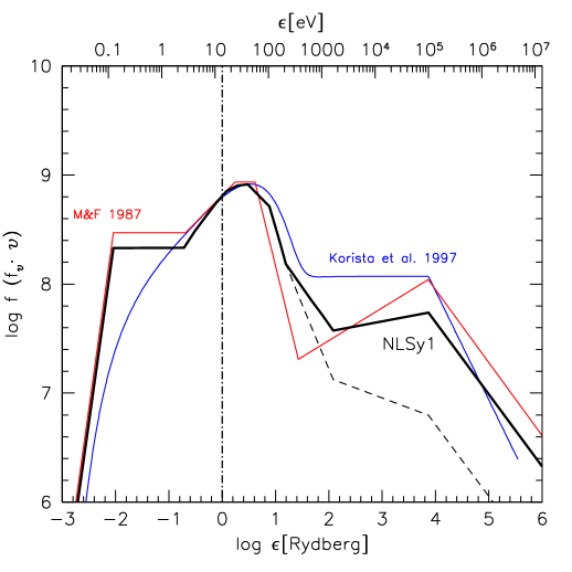
Figure 12: Continuum shapes employed for the evaluation of the error budget, with emitted power in arbitrary units as a function of photon energy in Ryd (lower $x$-axis) and in keV (upper $x$-axis). The thick solid line (NLSy1) is a SED appropriate for highly-accreting quasars; see text for a description of its construction. The dashed line traces the steepest continuum due to source by source diversity (i.e., the continuum of the most extreme Pop. A sources). The red and blue lines trace the Mathews & Ferland (1987) and the Korista et al. (1997) continua, respectively.

– The product $U$$n_{\mathrm{H}}$ value entered in Eq. 6 comes from dedicated sets of photoionization simulations that assume Mathews & Ferland (1987) continuum which is thought to be appropriate for Pop. A sources. However, the values of $\kappa$, $\bar{\nu_{\mathrm{i}}}$, and hence of factor $\kappa/\bar{\nu_{\rm i}}$ depend on the shape of the assumed photoionizing continuum. Extreme sources are expected to converge toward large values of $\Gamma_{\mathrm{soft}}$ (e.g., Boller et al., 1996; Wang et al., 1996; Grupe et al., 1999; Sulentic et al., 2000a; Grupe et al., 2010; Ai et al., 2011). In order to investigate the effect of different continua we considered a typical NLSy1 continuum as proposed by Grupe et al. (2010, Fig. 12). The average $\Gamma_{\mathrm{soft}}$ derived by Panessa et al. (2011) was assumed for energies larger than 20 keV. The dashed line shows a second “minimum” continuum representative of sources with $\Gamma_{\mathrm{hard}}\approx$ 2.2, computed on the basis of the observed dispersion in photon indexes up to 100 keV (Nikolajuk et al., 2004; Wang et al., 2013). The “standard” Mathews & Ferland (1987) and (Korista et al., 1997) were also considered as suitable for Pop. A sources. The scatter in $\log(\kappa/\bar{\nu_{\rm i}})$ derived from the values of the four continua is 0.033. We report this value in Table 4. A more appropriate range is probably between the NLSy1 continuum and the “minimum” spectral energy distribution (SED) of Fig. 12: if so, the scatter will be reduced to 0.02. This prediction should be tested by an analysis of low-$z$ sources for which X-ray data are available.

Factor ${n_{\mathrm{H}}U}$ –

The term ${n_{\mathrm{H}}U}$ is only slightly affected by the frequency redistribution of ionizing continua (within the continua assumed). However, $\log{n_{\mathrm{H}}U}$ depends on the diagnostic ratios values. cloudy 13 simulations (Ferland et al., 2013) indicate a difference of $\Delta\log{n_{\mathrm{H}}U}\approx 0.2$ from ratio Aliii$\lambda$1860/Siiii]$\lambda$1892$\approx$ 0.5 (A3^m) and Aliii$\lambda$1860/Siiii]$\lambda$1892$\approx$ 1.0 (A4^m). Since we do not actually separate A3^m and A4^m sources, we consider the difference as a source of statistical error $\pm 0.1$ around an average value. A proper treatment of the difference as a systematic effect will require a larger sample (§6.2). The measures of Negrete et al. (2013) on high S/N spectra indicate that measurement errors can be reduced to $\Delta\log{n_{\mathrm{H}}U}\approx 0.05$.

The structure factor $f_{\mathrm{S}}$

– The value of $f_{\mathrm{S}}$ is probably governed by $\lambda_{\mathrm{Edd}}$  (Netzer & Marziani, 2010). An upper limit variance was estimated by considering sources observed in reverberation mapping for which $M_{\rm BH}$ has been also derived from the $M_{\rm BH}$ – bulge velocity dispersion relation (Onken et al., 2004). The resulting uncertainty $\delta f_{\mathrm{S}}/f_{\mathrm{S}}\approx 0.2$ was derived from an heterogeneous sample of sources whose emission line profiles and accretion rate are very different (Negrete et al., 2013). The H$\beta$  profiles of xA sources can be almost always modeled with an unshifted (virial) Lorentzian component plus an additional component affecting the line base. This suggests the same, reproducible structure. We therefore expect a significantly smaller $\delta f_{\mathrm{S}}/f_{\mathrm{S}}$, $\rightarrow$ 0, if xA sources are considered as a distinct population in the analysis of the $M_{\rm BH}$ – bulge velocity dispersion relation, and assume $\delta f_{\mathrm{S}}/f_{\mathrm{S}}=0.1$ in Col. 3 of Table 4.

FWHM

– Eq. 6 suggests that a most relevant source of statistical error may be $\delta v$ that appears at the fourth power and is assumed here to be represented by the FWHM of H$\beta$  and intermediate ionization lines Aliii$\lambda$1860 and Siiii]$\lambda$1892 (§2). Indeed, a large fraction of the rms in the present sample can be accounted for by FWHM measurement errors, especially in sample 3. In Table 4 we conservatively estimate a typical error $\approx$15% in FWHM measures. A lower, $\approx$ 5% uncertainty in FWHM is within reach of dedicated observations.

6.1.2 $z$-based luminosity

Aperture effects

– Aperture losses and errors associated to the spectrophotometric calibration should be carefully assessed. Here we conservatively set a 1-$\sigma$ confidence error of 10% following the SDSS website.

Redshift $z$

– Detailed fitting can provide accurate redshift making the uncertainty on $z$ negligible. However, $z$-values provided by the survey suffer from significant uncertainties (Hewett & Wild, 2010). We assume a $\delta z\approx 0.002$. This uncertainty should be easily reduced to 0 by precise $z$ measures unless quasars show significant peculiar velocities with respect to the Hubble flow.

Bolometric correction

– The continuum shape has been represented here by a typical parameterization thought to be suitable for Pop. A sources (Mathews & Ferland, 1987) that are moderate/high Eddington radiators, with a single bolometric correction applied to all sources. The dispersion around the assumed value has been estimated to be $\approx$ 20% by Richards et al. (2006) for quasars of all spectral types. The dispersion around the typical spectral energy distribution of xA sources is probably lower. The main argument for a small scatter is again that we are considering objects thought to be producing similar emission line ratios. These ratios are dependent on the shape of the continuum (Negrete et al., 2012), making it reasonable to assume that the continua of xA sources are similar and with a dispersion significantly less than the one found in general surveys that do not distinguish spectral types. We derive a difference of $\approx$ 10% between the NLSy1 SED and the minimum SED in Fig. 12.

Continuum anisotropy

If the optical/UV continuum is emitted by an accretion disk, the observed luminosity should be dependent on the angle $\theta$ between the disk axis and the line of sight, which will be different for each source. The angular dependence can be written as $\lambda L_{\lambda}\approx\lambda L_{\lambda,\theta=0^{\circ}}\cos\theta(1+a_{1}\cos\theta)$, where the second term is the limb-darkening effect (e.g., Netzer et al., 1992; Netzer & Trakhtenbrot, 2014, in the case of a thin disk). The limb-darkening is wavelength dependent, and we are not aware of any exhaustive calculation in the context of slim disks (Watarai et al., 2001). Nonetheless slim disks are optically thick thermal radiators so that a good starting point is to consider them Lambertian radiators i.e., to first neglect the unknown but second order limb darkening effect, and then apply a reasonable limb darkening term $a_{1}\approx 2$  (Netzer & Trakhtenbrot, 2014). We estimate that anisotropy introduces a scatter of $\delta\log L\approx 0.085$, if the probability of observing a source at $\theta$ is $\propto\sin\theta$ with $0^{\circ}\leq\theta\leq 45^{\circ}$ in the case of a thin disk with no limb darkening effect. The scatter increases to $\delta\log L\la 0.15$ in the case of a slim disk whose height is assumed to scale with radius for dimensionless accretion rate $\dot{m}=1$ (Abramowicz et al., 1988, 1997).

6.1.3 Conclusion on statistical errors

The error sources described above and reported in Col. 2 of Table 4  provide a total error that accounts for and even exceeds the observed rms. The observed dispersion $\approx$0.365 implies that dispersion values reported in Table 4 might be close to the lowest values. Observational improvements can be devised to reduce, whenever possible, the main source of statistical errors that remains the FWHM of virial broadening estimator. Lowering FWHM measurements to $\approx$5%  would results in rms $\approx$ 0.3. This rms values is obtainable without requiring advancements in our physical understanding and in the connection of Eddington ratio to observed properties. If the scatter in Eddington ratio could be reduced by accounting for systematic and random effects, then rms $\approx$ 0.2 would become possible.

6.2 Systematic errors

6.2.1 General considerations

Eq. 6 is probably not influenced by systematic errors except for an offset associated with the the assumed $\lambda_{\mathrm{Edd}}$, $\kappa$ ($n_{\mathrm{H}}$$U$), and $\bar{\nu_{\mathrm{i}}}$. The offset will affect only $H_{0}$. There are also systematic effects that could reduce $z$-derived source luminosities. Light losses will also lead to systematic underestimates for luminosity which will affect $H_{0}$. Eq. 6 currently provides a valid redshift-independent luminosity estimator suited for the measure of $\Omega_{\mathrm{M}}$ and $\Omega_{\Lambda}$ only.

6.2.2 Orientation bias

Under the assumption that observed line broadening $\delta v_{\mathrm{obs}}$ is due to an isotropic component $\delta v_{\mathrm{iso}}$ plus a planar Keplerian component $v_{\mathrm{K}}$, the broadening can be expressed as $\delta v^{2}_{\mathrm{obs}}=\delta v^{2}_{\mathrm{iso}}+v^{2}_{\mathrm{K}}\sin^{2}\theta$ (e.g. Collin et al., 2006). The probability of observing a randomly-oriented source at $i$ is $\sin\theta$, and the systematic offset in Eddington ratio can be computed by integrating the Eddington ratio values computed at $\delta v_{\mathrm{obs}}$ over their probability of occurrence for a fixed $v_{\mathrm{K}}$. Assuming $\delta v_{\mathrm{iso}}/\delta v_{\mathrm{K}}=\frac{1}{2}$, $5\lower 2.15277pt\hbox{$\;\buildrel<\over{\sim}\;$}\theta\lower 2.15277pt\hbox{$\;\buildrel<\over{\sim}\;$}45$ the offset in $L/L_{\rm Edd}$ is approximately a factor of 2. Therefore, the Eddington ratio we are considering (and whose distribution is shown in Fig. 5) could be subject to a substantial bias. However, since orientation effects are not included in $\lambda_{\mathrm{Edd}}$ computations and $\lambda_{\mathrm{Edd}}\propto 1/v^{2}$, a correction to the virial broadening estimator in Eq. 6 would be compensated by the change in $\lambda_{\mathrm{Edd}}$, leading to a net $\Delta\log L\approx 0.0$.

In this paper the $\lambda_{\mathrm{Edd}}$ dispersion reported in Tab. 4 already takes into account orientation effects since $\delta\lambda_{\mathrm{Edd}}$ has been estimated from the a posteriori computed distribution of $\lambda_{\mathrm{Edd}}$  that is broadened by the orientation effect. A more proper approach would be to derive an orientation angle for individual sources. xA sources likely possess strong radiatively-driven winds whose physics and effect on the line profile of a high-ionization line like Civ$\lambda$1549 can be modeled (Murray & Chiang, 1997; Proga et al., 2000; Risaliti & Elvis, 2010; Flohic et al., 2012).

6.2.3 Major expected systematic effects as a function of $z$, $L$, and sample selection criteria

In the 4DE1 approach luminosity dependences are in the parameters correlated with Eigenvector 2 (Boroson & Green, 1992). The main correlate is the equivalent width of Civ$\lambda$1549 (i.e., the well known “Baldwin effect”; Bian et al. e.g., 2012, and references therein). In that case, indeed, even if the most likely explanation of the decrease of W(Civ$\lambda$1549) with luminosity found in large sample is a dependence of W(Civ$\lambda$1549) on Eddington ratio plus selection effects in flux limited sample (Baskin & Laor, 2004; Bachev et al., 2004; Marziani et al., 2008), the Civ$\lambda$1549 equivalent width should be avoided because of a possible residual dependence with luminosity. The diagnostic ratios we employ are meant to minimize any possible dependence from a physical parameter that is in turn related to luminosity, like for example the covering fraction of the emitting gas that may affect W(Civ$\lambda$1549).

Neither $R_{\rm FeII}$ nor Aliii$\lambda$1860/Siiii]$\lambda$1892 depend significantly on $z$ or luminosity in xA sources. Selecting xA sources from the Shen et al. (2011) sample, correlation coefficients are not significantly different from 0. For 378 sources with $R_{\rm FeII}$$\geq$1, the Pearson correlation coefficients are 0.075 and 0.09 with $z$ and $L$ respectively. These values are both not significant even if the sample of sources is relatively large. The Aliii$\lambda$1860/Siiii]$\lambda$1892 ratio as a function of redshift and luminosity yields least-square fittings lines that not significantly different from 0. We have verified that the optical and UV selection criteria are mutually consistent in § 2.5, and shown that the conditions on $R_{\rm FeII}$ and Aliii$\lambda$1860 – Ciii]$\lambda$1909 are simultaneously satisfied over a wide range $L$ and $z$, even if for the only 9 xA sources with available data: from 1H 0707-495 (the lowest luminosity A3 source, $\log L\approx 44.6$ [ergs s^-1] at $z\approx 0.04$) to HE1347-2457 ($\log L\approx 47.9$, at $z\approx 2.599$).

Residual systematic effects can arise if the quantities entering Eq. 6 are different in high- and low-$z$ sources i.e., in $R_{\rm FeII}$-selected and 1900 -selected samples.

$L/L_{\rm Edd}$—

Our present $N=$92 sample suffers from a slight $L/L_{\rm Edd}$ bias. The difference in $L/L_{\rm Edd}$ between sample 1 and 3 (optical and UV based) indicates that $\delta\log$ $L/L_{\rm Edd}$$\la 0.08$.

Several works suggest a relation between diagnostic ratios $R_{\rm FeII}$, Aliii$\lambda$1860/ Siiii]$\lambda$1892 and Siiii]$\lambda$1892/Ciii]$\lambda$1909, and Eddington ratio (Marziani et al., 2003c; Shen et al., 2011; Aoki & Yoshida, 1999; Wills et al., 1999). There is no correlation at all between $R_{\rm FeII}$ and the UV ratios employed in this paper as far as the general population of AGNs is concerned (Fig. 4). However this may not be longer true when $R_{\rm FeII}$$\rightarrow 1$: if $R_{\rm FeII}$$\approx$1, Aliii$\lambda$1860/Siiii]$\lambda$1892$\approx$0.5 and Ciii]$\lambda$1909/Siiii]$\lambda$1892$\approx$1, while for larger $R_{\rm FeII}$ Aliii$\lambda$1860 becomes stronger and Ciii]$\lambda$1909 weaker. Indeed, 4DE1 suggests a relation between $L/L_{\rm Edd}$ and metallicity, with the most metal rich system being associated only with the sources accreting at the highest rate. An important result of the present investigation is right that xA sources – that are extremely metal rich (Negrete et al., 2012) – are revealed over a broad range of $L$ and $z$, but only for a very narrow range of $L/L_{\rm Edd}$. As stressed earlier, luminosity and $z$ cannot be major correlates.

As long as the distribution of the measured intensity ratios Aliii$\lambda$1860/Siiii]$\lambda$1892, Siiii]$\lambda$1892/Ciii]$\lambda$1909 and $R_{\rm FeII}$ are independent of $z$  and $L$ (absence of even a weak correlation could be enforced by resampling to avoid small effects), a relation (if any) between $R_{\rm FeII}$ and Aliii$\lambda$1860/Siiii]$\lambda$1892, Siiii]$\lambda$1892/Ciii]$\lambda$1909 is established, inter-sample systematic effects should be minimized. The 9 sources considered in §2.5 are clearly insufficient to test these conditions. A proper observational strategy could involve: (1) a large sample to define a relation between $R_{\rm FeII}$ and Aliii$\lambda$1860/Siii$\lambda$1814, Siiii]$\lambda$1892/Ciii]$\lambda$1909  (and $L/L_{\rm Edd}$). This is especially needed since any $\lambda_{\mathrm{Edd}}$ deviation as a function of redshift can introduce a significant systematic effect: for example, $\delta\log$$L/L_{\rm Edd}$$\approx-0.05$ between sample 3 and 1 implies $\delta$$\Omega_{\mathrm{M}}$$\approx$ 0.05; (2) a vetted subsample with H$\beta$ observations in the near IR and simultaneous 1900 observations in the optical.

$\kappa/h\bar{\nu}$ —

A change of ionizing continuum shape as a function of redshift and/or luminosity, namely of the ratio $\kappa/h\bar{\nu}_{i}$  for a fixed Aliii$\lambda$1860/ Siiii]$\lambda$1892, Siiii]$\lambda$1892/ Ciii]$\lambda$1909 and $R_{\rm FeII}$. This could occur, practically, if we were selecting more and more extreme objects with the steepest continua. The properties of the ionizing continuum in quasars are not very well known; however, it is reasonable to assume that Pop. A sources show continua intermediate between the continuua shown in Fig. 12. If the continua labeled as Korista et al. (1997) and the extreme, minimum NLSy1 continuum (dashed line) are considered, $\kappa/h\bar{\nu}_{i}$ will change from 0.174 to 0.207, with a $\delta\log L\approx 0.075$. xA sources are expected to show a steep X-ray continuum (Grupe et al., 2010; Panessa et al., 2011; Wang et al., 2013), so that the range of change may be more realistically bracketed by the typical NLSy1 and minimum continuum. In this case, the hypothesis of a systematic evolution implies a change in $\kappa/h\bar{\nu}_{i}$ that leads to $\delta\log L\approx 0.035$. However, the change in $n_{\mathrm{H}}$$U$ associated with different continua (for the same values of the observed Aliii$\lambda$1860/Siii$\lambda$1814 ratios) tends to compensate for the change in $\kappa/h\bar{\nu}_{i}$, reducing the effect to $\delta\log L\approx 0.026$. There is no evidence for such evolution/selection effects in xA sources, but the relevance of systematic continuum changes and the relation between $\kappa$ ($n_{\mathrm{H}}$$U$), and $\bar{\nu_{\mathrm{i}}}$ and diagnostic ratios should be tested with dedicated X-ray observations of high-$z$ xA sources.

Ionizing photon flux $n_{\mathrm{H}}$$U$ —

The factor $n_{\mathrm{H}}$$U$ is set by the Aliii$\lambda$1860/ Siiii]$\lambda$1892, Siiii]$\lambda$1892/ Ciii]$\lambda$1909 and $R_{\rm FeII}$ ratios and, for a given continuum shape, we do not expect systematic changes. When selecting large samples some degree of heterogeneity is unavoidable. Differences in the Eq. 6 parameter values for bins A3^m and A4^m will contribute to the overall sample rms but should not introduce any systematic effects as long as the fraction A3^m/A4^m or, more properly, the Aliii$\lambda$1860/ Siiii]$\lambda$1892, Siiii]$\lambda$1892/ Ciii]$\lambda$1909 and $R_{\rm FeII}$  distributions are consistent and independent from $z$.

Structure factor $f_{\mathrm{S}}$

– The self-similarity of the profiles over $z$ and luminosity should be carefully tested on high S/N spectra since the FWHM of the lines is clearly dependent on the assumed profile shape. Available data support the assumption that the shape is not changing as a function of FWHM and $z$ (as also shown by the data of Fig. 2 and Fig. 3): a Lorentzian function yielded good fits for H$\beta$, Aliii$\lambda$1860, Siii$\lambda$1814 in all cases considered in this paper. This is also true when fits are made to carefully selected composite spectra with S/N $\ga$100 (see e.g., Zamfir et al., 2010).

An important systematic effect is related to the use of equation determination of the quasar luminosity from redshift (Eq. 8).

$B.C.(1800)--B.C.(5100)$ —

The ratio between the bolometric correction at 5100 Å and 1800 Å has been assumed in this paper to be $\lambda f_{\lambda}(5100)/\lambda f_{\lambda}(1800)$ = 0.63 on the basis of the Mathews & Ferland (1987) continuum. A more proper value could be well 0.7, as measured on the optical and UV spectral of I Zw1. This change will shift the estimate of $\Omega_{\mathrm{M}}$ by $\approx$ 0.05, to $\Omega_{\mathrm{M}}$$\approx$ 0.25, in the case of constrained $\Omega_{\mathrm{M}}$+ $\Omega_{\Lambda}$= 1.0. In addition if $\lambda f_{\lambda}(5100)/\lambda f_{\lambda}(1800)\approx$  0.7 the systematic offset in the $L/L_{\rm Edd}$ distribution between sample 1 and 3 will be reduced by $\approx$ 0.05. The average ratio $\lambda f_{\lambda}(5100)/\lambda f_{\lambda}(1800)$  and the associated dispersion (and hence $B.C.(1800)--B.C.(5100)$) should be carefully established by dedicated observations. Such observations are also needed because continuum anisotropy leads, in addition to a random error, to a systematic underestimate of source luminosity, as discussed below. The effect is relevant here as long as it is wavelength dependent if optical and UV data are considered together. Recent observational work on radio-loud sources suggests that the degree of anisotropy changes very little with wavelength (Runnoe et al., 2013). However, this may not be the case for slim disks of highly accreting sources.

The most relevant systematic effects, among the ones that are listed above, are related to $B.C.(1800)/B.C.(5100)$ and to the distributions of the optical and UV line ratios that could be linked to small – but significant – trends in $L/L_{\rm Edd}$. We have shown that other effects, like evolution of the ionising continuum – within reasonable limits – may yield a modest systematic effect on luminosity estimates, $\approx$ 0.03 dex.

The following effects are more speculative in nature and of lower relevance.

• Continuum anisotropy is also expected to give rise to a Malmquist-type bias in $z$ based luminosities. Close to a survey limiting magnitude the brightest (face-on) sources will be selected preferentially. Unlike relativistic beaming however, disk anisotropy is of relatively modest amplitude. In the case of a slim disk with limb darkening the difference between a face-on source and a randomly oriented sample of objects is $\delta\log L\approx 0.2$ dex. Since core-dominated radio-loud sources are expected to have an additional relativistically beamed synchrotron continuum component, they should be avoided from any sample. If sources are selected from a large flux limited sample, (1) either orientation is inferred from Civ$\lambda$1549 line profile modelling, or (2) a more elementary precaution would be to consider sources brighter than $\approx 0.5$  mag than their discovery survey (i.e., the SDSS in the case of sample 3 limiting magnitude).

• Intervening large scale structures are expected to produce a lensing effect on the light emitted by distant quasars. This effect is noticeable especially for sources at $z\ga$1 (Holz & Wald, 1998; Holz & Linder, 2005). The lensing effect is however found to be averaged out for large samples ($\la 100$ sources) which is the case of any quasar sample that could be realistically employed for cosmology.

The present samples hint at (small) systematic differences that can be more clearly revealed and quantified only with a larger sample and/or vetted. As long as we employ the same diagnostic ratios (with consistent distributions of values as a function of $z$) and the same line profile model, residual systematic effects with $z$, $L$, and $L/L_{\rm Edd}$should be minimized. Any systematic change with $z$ and $L$  affecting the parameters entering into Eq. 6 will also affect the intensity ratios and will become detectable. Assessing and avoiding systematic effects would require a uniform redshift coverage, as assumed for the mock samples. More details on a possible observational strategy are give in §7.2.

7 Discussion

The idea to use quasars as Eddington standard candles is not new (e.g., Marziani et al., 2003a; Teerikorpi, 2005; Bartelmann et al., 2009; Sulentic et al., 2012; Wang et al., 2013). Luminosity correlations were the past great hope for using quasars as standard candles. The most promising luminosity correlation involved the Baldwin effect (Baldwin, 1977; Baldwin et al., 1978) which is now thought to be governed by Eddington ratio (Bachev et al., 2004; Baskin & Laor, 2004). In any case it is too weak to provide interesting cosmological constraints. Other methods using line width measures have also been proposed (e.g., Rudge & Raine, 1999) although it is unclear that the line width distribution shows real change with redshift. Recently, a somewhat similar proposal to the one presented in this paper has been advanced which advocates the hard X-ray spectra index as a selector for extreme sources (Wang et al., 2013). We considered both hard and soft X-ray measures when selecting the principal 4DE1 parameters and concluded that hard measures showed too little dispersion across the 4DE1 optical plane compared to $\Gamma_{\mathrm{soft}}$ (Sulentic et al., 2000b).

The concordance $H_{0}$ value has to be assigned a priori to constrain $\Omega_{\mathrm{M}}$ and $\Omega_{\Lambda}$  to avoid circularity, unless the normalised slope is used as a best-fit estimator. The determination of $H_{0}$ is not fully independent of $z$-based distances. The Eddington ratio estimate for I Zw 1 requires a luminosity computation that assumes a value of $H_{0}$. In order to make an independent determination of $\lambda_{\mathrm{Edd}}$ (and hence of $H_{0}$) at least one redshift independent luminosity determination would be needed (e.g. distance inferred from a type Ia supernova). In this case $M_{\rm BH}$ would follow from luminosity via the virial relation with $r\propto L^{1/2}$ and $L/L_{\rm Edd}$ from the ratio $L$/$M_{\rm BH}$. Another approach would be to derive $\lambda_{\mathrm{Edd}}$ from a physical model of the high-ionization outflow common to extreme Eddington sources.

The definition of ionization parameter also involves $L$. However ionization parameter and density values were derived from emission line ratios. The luminosity is a theoretical luminosity that, for an assumed continuum, yields the number of ionizing photons needed to produce the emission lines. We retrieve $Un_{\mathrm{H}}$ from emission line ratios; no flux or line luminosity measurements are involved. The assumption that $r\propto L^{0.5}$ is consistent with the assumption of $Un_{\mathrm{H}}$ = const (actually, it follows from the definition of $U$). Therefore, Eq. 6 has no implicit circularity.

7.1 Comparison with the Supernova Legacy Survey

There are many analogies between supernova surveys (Guy et al., 2010) and our proposed method using quasars. Both methods rely on intrinsic luminosity estimates for a large number of discrete sources. The advantage of the supernova surveys is that individual supernovæ show a smaller scatter in luminosity (e.g., Riess et al., 2001). However, very few supernovæ have been detected at $z\ga 1$ while a quasars sample can be easily extended (with significant numbers) to $z\approx 3$ or possibly $z\approx 4$. Differences in redshift coverage account for the different sensitivity to $\Lambda$: $\Omega_{\Lambda}$ is tightly constrained using supernovæ while it remains loosely constrained using quasars. Quasars are distributed over a redshift range where $\Omega_{\mathrm{M}}$ ruled the expansion of the Universe while supernovæ sample epochs of accelerated expansion (Fig. 6). But quasars can sample any range covered by supernovæ. Statistical errors for $\Omega_{\mathrm{M}}$ derived from the mock samples (with unconstrained $\Omega_{\mathrm{M}}$ and $\Omega_{\Lambda}$) are lower than ones derived from the first three years of the supernova legacy survey that yield $\Omega_{\mathrm{M}}$$\approx 0.19^{+0.08}_{-0.10}$ (Conley et al., 2011).

7.2 Possible observational strategies

In order to exploit a sample of high $L/L_{\rm Edd}$ radiators both calibration observations and a larger sample of extreme Eddington sources are needed. Simultaneous rest frame UV and optical observations covering the 1900 and H$\beta$ range are needed (a feat within the reach of present day multi-branch spectrometers): (1) to constrain the bolometric corrections and specifically the $B.C.(1800)/B.C.(5100)$ ratio; (2) to define systematic differences between spectral types A3^m and A4^m, including the $B.C.$ An attempt should be also made to cover with a large H$\beta$ sample the $z$ range 0.1 – 1.5, where the effect of a nonzero $\Omega_{\Lambda}$ is most noticeable and where any rest-frame optical/UV inter calibration is not needed. A related option is to obtain $R_{\rm FeII}$  only, covering the redshifted H$\beta$ spectral range into the near and mid IR ($K$ band observations can reach $z\approx 3.5$). Alternatively, the UV 1900 blend can be easily covered by optical spectrometers over the redshift range 1.1 $\la z\leq 3.5$. This approach would allow to measure $\Omega_{\mathrm{M}}$ without the encumbrance of an inter calibration with H$\beta$  data.

The best hope for accurate and precise results rests in a “brute force” application of the method to a large sample. Tab. 4 shows that rms$\approx$ 0.3 can be obtained with better data. With uniform redshift coverage the precision of the method will scale with rms/$\sqrt{N}$. This means that a precision similar to the one obtained with the mock sample (rms = 0.2) can be achieved with a sample of 400 sources while a precision similar to rms = 0.1 would require a sample near 1000 quasars. It is possible that a sample of this size (or even larger) can be selected from spectra collected by recent major optical surveys (e.g., Pâris et al., 2012).

8 Conclusion

We have shown that sources radiating at, or close to, $L/L_{\rm Edd}$$\approx$1 can be identified in significant numbers with reasonable confidence. These sources show stable emission line ratios over a very wide range of $z$ and $L$. We have performed exploratory computations and shown that these sources – apart from their intrinsic importance for quasar physics – may be also prime candidates as cosmological probes. We then presented a method for using some quasars as redshift-independent distance estimators. We do not claim to present constraining results in this paper beyond showing an overall consistency with concordance cosmology and exclusion of extreme models (e.g. a flat Universe dominated by the cosmological constant) starting from an estimates of the most likely values of quasar physical parameters entering in Eq. 6. Our goal was to identify suitable quasars, to describe a possible approach capable of yielding meaningful constraints on $\Omega_{\mathrm{M}}$ and $\Omega_{\Lambda}$, and to identify most serious statistical and systematic sources of uncertainty. A quantitative analysis of systematic effects due to continuum shape, orientation, $f_{\mathrm{S}}$  and $\lambda_{\mathrm{Edd}}$ as well as an attempt at reducing statistical errors is deferred to further work. Addressing and overcoming systematic biases requires dedicated, but feasible, new observations.

We stress that the precision of our method can be greatly improved with high S/N spectroscopic observations for significant samples of quasars. This is not just the usual refrain claiming that improvement in S/N can lead to unspecified advancements: previous work shows that broad-line FWHM for Pop. A sources can be measured with a typical accuracy of 10% at a 2$\sigma$ confidence level. This would represent a major improvement with respect to the 20% at 1$\sigma$ uncertainty for many FWHM values used in this work – implying $\Delta\log L$ errors decreasing from $\approx 0.7$ to $\lower 2.15277pt\hbox{$\;\buildrel<\over{\sim}\;$}0.1$. Figs. 10 and 11 shows that cosmologically meaningful limits can be set even with currently obtainable data.

PM and JS acknowledge support from la Junta de Andalucía, through grant TIC-114, Proyectos de Excelencias P08-FQM-04205 + P08-TIC-3531 as well as the Spanish Ministry for Science and Innovation through grant AYA2010-15169.

Funding for the SDSS and SDSS-II has been provided by the Alfred P. Sloan Foundation, the Participating Institutions, the National Science Foundation, the U.S. Department of Energy, the National Aeronautics and Space Administration, the Japanese Monbukagakusho, the Max Planck Society, and the Higher Education Funding Council for England. The SDSS Web Site is http://www.sdss.org/.

The SDSS is managed by the Astrophysical Research Consortium for the Participating Institutions. The Participating Institutions are the American Museum of Natural History, Astrophysical Institute Potsdam, University of Basel, University of Cambridge, Case Western Reserve University, University of Chicago, Drexel University, Fermilab, the Institute for Advanced Study, the Japan Participation Group, Johns Hopkins University, the Joint Institute for Nuclear Astrophysics, the Kavli Institute for Particle Astrophysics and Cosmology, the Korean Scientist Group, the Chinese Academy of Sciences (LAMOST), Los Alamos National Laboratory, the Max-Planck-Institute for Astronomy (MPIA), the Max-Planck-Institute for Astrophysics (MPA), New Mexico State University, Ohio State University, University of Pittsburgh, University of Portsmouth, Princeton University, the United States Naval Observatory, and the University of Washington.

Table 1: Measured quantities for the H$\beta$ based samples

Source	$z^{\mathrm{a}}$	$\lambda f_{\lambda}^{\mathrm{b}}$	S/N	FWHM	$\delta$FWHMc	Sample
		[ergs s-1cm-2]		[km s-1]	[km s-1]
SDSSJ014247.74-084517.5	0.571	3.23E-12	15	2230	220	1
SDSSJ030000.01-080356.9	0.562	7.31E-12	36	2100	210	1a
SDSSJ074840.52+154456.8	0.469	4.50E-12	25	2450	250	1
SDSSJ080908.14+461925.6	0.657	6.34E-12	23	2290	230	1
SDSSJ082024.22+233450.4	0.470	3.12E-12	25	1720	170	1
SDSSJ085557.11+561534.7	0.715	6.49E-12	25	2680	270	1a
SDSSJ090423.31+400704.7	0.410	4.27E-12	20	1870	190	1
SDSSJ090840.71+132117.3	0.458	2.40E-12	16	2370	240	1
SDSSJ093531.61+354101.0	0.494	4.58E-12	18	2140	210	1a
SDSSJ094033.76+462315.0	0.696	4.58E-12	15	2010	200	1
SDSSJ103457.27+235638.1	0.419	2.39E-12	21	1420	140	1
SDSSJ104613.73+525554.2	0.503	2.94E-12	22	1790	180	1
SDSSJ104817.98+312905.8	0.452	5.19E-12	20	1870	190	1
SDSSJ105205.58+364039.6	0.609	5.76E-12	35	2330	230	1a
SDSSJ105600.08+142411.3	0.623	3.94E-12	24	2500	250	1
SDSSJ110312.93+414154.9	0.402	1.01E-11	34	2050	210	1
SDSSJ110406.94+314111.5	0.434	5.02E-12	36	2030	200	1a
SDSSJ111909.51+153216.4	0.674	5.23E-12	24	2800	280	1a
SDSSJ112756.76+115427.1	0.510	4.76E-12	16	1820	180	1
SDSSJ112757.41+644118.4	0.695	4.03E-12	17	1850	190	1
SDSSJ113338.64+220026.8	0.546	2.78E-12	17	2080	210	1
SDSSJ113625.42+100523.2	0.552	3.13E-12	20	1460	150	1
SDSSJ113944.64+121436.0	0.618	3.01E-12	17	1420	140	1
SDSSJ120633.07+412536.1	0.554	4.87E-12	21	2110	210	1a
SDSSJ120734.63+150643.6	0.750	4.51E-12	19	2240	220	1
SDSSJ121850.52+101554.1	0.543	4.06E-12	25	1700	170	1a
SDSSJ122557.86+364907.7	0.477	3.77E-12	22	2210	220	1
SDSSJ124511.25+335610.1	0.711	7.21E-12	20	2270	230	1
SDSSJ130112.93+590206.7	0.476	1.66E-11	42	2250	230	1

• Redshift provided in the SDSS file header.

• At 5100 Å rest frame.

• 1 $\sigma$ confidence level.

Table 1: (cont.) Measured quantities for the H$\beta$ based samples

Source	$z^{\mathrm{a}}$	$\lambda f_{\lambda}^{\mathrm{b}}$	S/N	FWHM	$\delta$FWHMc	Sample
		[ergs s-1cm-2]		[km s-1]	[km s-1]
SDSSJ130357.42+103313.5	0.589	3.87E-12	21	2210	220	1
SDSSJ132048.67+510313.7	0.466	4.74E-12	48	2040	200	1a
SDSSJ133225.99+151926.4	0.466	3.55E-12	24	2160	220	1
SDSSJ133602.01+172513.1	0.552	9.66E-12	15	2440	240	1
SDSSJ143123.67+202142.8	0.578	3.12E-12	17	2240	220	1a
SDSSJ143633.75+065655.0	0.400	2.87E-12	49	1690	170	1
SDSSJ144448.25+234554.3	0.629	3.14E-12	17	2800	280	1a
SDSSJ144733.05+345506.7	0.662	8.31E-12	41	2300	230	1a
SDSSJ145543.45+300322.3	0.629	2.96E-12	18	2140	210	1
SDSSJ154333.94+102231.9	0.487	4.40E-12	29	2250	220	1
SDSSJ154823.46+141407.8	0.581	3.04E-12	24	1890	190	1a
SDSSJ161924.11+260907.2	0.629	4.80E-12	25	2400	240	1
SDSSJ162817.12+200348.7	0.571	3.59E-12	16	2220	220	1
SDSSJ165722.08+395551.4	0.579	3.01E-12	16	2400	240	1
HE0122-3759	2.200	1.44E-11	77	3400	300	2
HE0359-3959	1.521	9.18E-12	40	4250	400	2
HE1003+0149	1.080	9.89E-12	32	2900	300	2
HE1347-2457	2.599	1.88E-11	25	6500	600	2
HE1430-0041	1.122	8.42E-12	40	4720	300	2
HE1505+0212	1.094	1.41E-11	81	5230	200	2
HE2305-5315	1.073	1.68E-11	50	3300	500	2

• Redshift provided in the SDSS file header.

• At 5100 Å rest frame.

• 1 $\sigma$ confidence level.

Table 2: Measured quantities for the Aliii$\lambda$1860 based samples

Source	$z^{\mathrm{a}}$	$\lambda f_{\lambda}^{\mathrm{b}}$	S/N	FWHM	$\delta$FWHMc	Sample
		[ergs s-1cm-2]		[km s-1]	[km s-1]
SDSSJ013514.52-005319.0	2.113	6.13E-12	15	3440	800	3
SDSSJ073149.53+284357.1	2.227	1.25E-11	17	4480	1100	3
SDSSJ075220.38+165506.6	2.109	7.70E-12	24	5320	900	3
SDSSJ081717.14+370252.0	2.064	1.03E-11	23	3500	400	3
SDSSJ082936.31+080140.6	2.196	1.10E-11	21	4970	500	3
SDSSJ084258.83+361444.2	2.490	8.79E-12	22	2850	400	3
SDSSJ084502.73+081214.2	2.348	7.87E-12	15	4860	600	3
SDSSJ084525.84+072222.3	2.306	1.36E-11	21	3700	900	3
SDSSJ085406.12+423810.7	2.386	6.32E-12	16	5110	600	3
SDSSJ091942.82+340301.3	2.447	1.12E-11	20	5120	900	3
SDSSJ093403.96+315331.3	2.422	2.16E-11	30	3850	900	3
SDSSJ094144.72+231144.2	2.541	1.18E-11	22	3660	900	3
SDSSJ094707.81+481613.8	2.439	1.10E-11	20	5100	900	3
SDSS J094748.07+193920.0	2.255	1.20E-11	18	5700	500	3
SDSSJ095707.82+184739.9	2.341	1.78E-11	29	3520	900	3
SDSSJ095817.81+494618.3	2.352	9.63E-12	21	4500	900	3
SDSSJ100356.15-005940.4	2.107	6.07E-12	16	4250	1100	3
SDSSJ100459.14+470058.0	2.577	1.54E-11	29	4900	900	3
SDSSJ100513.60+004028.4	2.557	1.95E-11	18	3280	300	3
SDSSJ104930.88+543839.7	2.549	1.18E-11	19	5380	500	3
SDSSJ105427.17+253600.8	2.400	1.53E-11	23	3780	900	3
SDSSJ111154.35+372321.2	2.058	1.44E-11	25	5470	900	3
SDSSJ112140.13+322346.6	2.177	1.56E-11	22	3170	300	3
SDSSJ114925.65+665949.4	2.240	9.39E-12	29	4290	900	3
SDSSJ120821.01+090130.3	2.075	1.24E-11	24	3920	900	3
SDSSJ122709.48+310749.3	2.173	1.33E-11	19	4890	900	3
SDSSJ125257.96+274542.4	2.001	6.89E-12	19	4420	500	3
SDSSJ125914.85+672011.8	2.443	1.34E-11	25	3060	400	3
SDSSJ125924.28+445105.0	2.030	1.80E-11	28	2780	400	3

• Redshift provided in the SDSS file header.

• At 1800 Å rest frame.

• 1 $\sigma$ confidence level.

Table 2: (cont.) Measured quantities for the Aliii$\lambda$1860 based samples

Source	$z^{\mathrm{a}}$	$\lambda f_{\lambda}^{\mathrm{b}}$	S/N	FWHM	$\delta$FWHMc	Sample
		[ergs s-1cm-2]		[km s-1]	[km s-1]
SDSSJ130236.17+095831.8	2.073	1.12E-11	22	5170	900	3
SDSSJ130924.78+412427.9	2.081	9.08E-12	17	2500	800	3
SDSSJ132615.16-030357.5	2.121	2.45E-11	33	5220	900	3
SDSSJ142402.65+263624.8	2.095	6.44E-12	17	5270	600	3
SDSSJ142500.24+494729.3	2.253	2.24E-11	24	4050	900	3
SDSSJ153837.01+522555.1	2.078	8.34E-12	18	3630	600	3
SDSSJ154624.57-014849.2	2.009	8.15E-12	18	3050	800	3
SDSSJ154757.71+060626.6	2.018	1.82E-11	35	4300	900	3
SDSSJ160955.41+065401.9	2.134	1.06E-11	22	4910	900	3
SDSSJ162115.06+400732.2	2.206	1.21E-11	47	2390	300	3
SDSSJ210831.56-063022.5	2.345	2.53E-11	61	5060	500	3
SDSSJ223304.01-080142.6	2.264	8.82E-12	17	4160	1100	3
SDSSJ232115.48+142131.5	2.537	1.05E-11	16	4260	1100	3

• Redshift provided in the SDSS file header.

• At 1800 Å rest frame.

• 1 $\sigma$ confidence level.

Table 3: Results from Preliminary Sample

Selected Cosmologies
		$\bar{\Delta}/\sigma_{\bar{\Delta}}^{a}$	$b^{b}$	$\chi^{2}~{}^{c}$
Concordance		1.21	0.03	1.05
$\Lambda$-dominated		-6.53	-0.18	1.67
M-dominated		-0.12	0.125	1.84
Little Matter		1.74	-0.03	1.07
Empty		0.64	0.06	1.06

• Ratio between the average of $\delta\log L$ and the average standard deviation.

• Slope of linear fit. For our sample, $\sigma_{b}\approx 0.075$.

• Normalized $\chi^{2}$.

Table 4: Error Budget

Parameter $p$	$\delta\log p^{a}$	Power
	Virial luminosity
$\lambda_{\mathrm{Edd}}$	0.13	2
$\kappa/(\bar{\nu_{\mathrm{i}}})$	0.020 – 0.033	1
$10^{n_{\mathrm{H}}U}$	0.050 – 0.100	1
$f_{\mathrm{S}}$	0.043 – 0.087	2
FWHM	0.065	4
Prop. err.	0.379 – 0.418
	$z$-based luminosity
$f_{\lambda}$	0.043	1
$z$	0.000 – 0.001	2
$B.C.$	0.043 – 0.087	1
Anisotropy	0.085 – 0.15	1
Prop. err.	0.105 – 0.179
Total err.	0.394 – 0.455

• Estimated statical errors for the actual sample of 92 sources presented in this paper.

Figure 6: Expected bolometric luminosity difference for several cosmological models, referenced to the case of an “empty” Universe (horizontal dot-dashed line) with $\Omega_{M}=0.00$, $\Omega_{\Lambda}=0.00$.

References

- Abramowicz et al. (1988) Abramowicz, M. A., Czerny, B., Lasota, J. P., & Szuszkiewicz, E. 1988, ApJ, 332, 646
- Abramowicz et al. (1997) Abramowicz, M. A., Lanza, A., & Percival, M. J. 1997, ApJ, 479, 179
- Ai et al. (2010) Ai, Y. L., Yuan, W., Zhou, H. Y., Wang, T. G., Dong, X.-B., Wang, J. G., & Lu, H. L. 2010, ApJL, 716, L31
- Ai et al. (2011) Ai, Y. L., Yuan, W., Zhou, H. Y., Wang, T. G., & Zhang, S. H. 2011, ApJ, 727, 31
- Allen et al. (2011) Allen, S. W., Evrard, A. E., & Mantz, A. B. 2011, ARAAp, 49, 409
- Aoki & Yoshida (1999) Aoki, K., & Yoshida, M. 1999, in Astronomical Society of the Pacific Conference Series, Vol. 162, Quasars and Cosmology, ed. G. Ferland & J. Baldwin, 385
- Assef et al. (2011) Assef, R. J., et al. 2011, ApJ, 742, 93
- Bachev et al. (2004) Bachev, R., Marziani, P., Sulentic, J. W., Zamanov, R., Calvani, M., & Dultzin-Hacyan, D. 2004, ApJ, 617, 171
- Baldwin (1977) Baldwin, J. A. 1977, ApJ, 214, 679
- Baldwin et al. (1978) Baldwin, J. A., Burke, W. L., Gaskell, C. M., & Wampler, E. J. 1978, Nature, 273, 431
- Baldwin et al. (2004) Baldwin, J. A., Ferland, G. J., Korista, K. T., Hamann, F., & LaCluyzé, A. 2004, ApJ, 615, 610
- Baldwin et al. (1996) Baldwin, J. A., et al. 1996, ApJ, 461, 664
- Bartelmann et al. (2009) Bartelmann, M., et al. 2009, in Questions of Modern Cosmology: Galileo’s Legacy, by D’Onofrio, Mauro; Burigana, Carlo, ISBN 978-3-642-00791-0. Berlin: Springer-Verlag Heidelberg, 2009, p. 7-202, ed. D’Onofrio, M. & Burigana, C. (Springer Verlag, Berlin-Heidelberg), 7–202
- Baskin & Laor (2004) Baskin, A., & Laor, A. 2004, MNRAS, 350, L31
- Bentz et al. (2009) Bentz, M. C., Peterson, B. M., Pogge, R. W., & Vestergaard, M. 2009, ApJL, 694, L166
- Bentz et al. (2013) Bentz, M. C., et al. 2013, ApJ, 767, 149
- Bevington (1969) Bevington, P. R. 1969, Data reduction and error analysis for the physical sciences (New York: McGraw-Hill)
- Bian et al. (2012) Bian, W.-H., Fang, L.-L., Huang, K.-L., & Wang, J.-M. 2012, MNRAS, 427, 2881
- Bochkarev & Gaskell (2009) Bochkarev, N. G., & Gaskell, C. M. 2009, Astronomy Letters, 35, 287
- Boller et al. (1996) Boller, T., Brandt, W. N., & Fink, H. 1996, AAp, 305, 53
- Boroson (2002) Boroson, T. A. 2002, ApJ, 565, 78
- Boroson & Green (1992) Boroson, T. A., & Green, R. F. 1992, ApJS, 80, 109
- Brühweiler & Verner (2008) Brühweiler, F., & Verner, E. 2008, ApJ, 675, 83
- Campbell et al. (2013) Campbell, H., et al. 2013, ApJ, 763, 88
- Chen & Wang (2004) Chen, L.-H., & Wang, J.-M. 2004, ApJ, 614, 101
- Collin et al. (2002) Collin, S., Boisson, C., Mouchet, M., Dumont, A.-M., Coupé, S., Porquet, D., & Rokaki, E. 2002, AAp, 388, 771
- Collin & Kawaguchi (2004) Collin, S., & Kawaguchi, T. 2004, AAp, 426, 797
- Collin et al. (2006) Collin, S., Kawaguchi, T., Peterson, B. M., & Vestergaard, M. 2006, A&Ap, 456, 75
- Conley et al. (2011) Conley, A., et al. 2011, ApJS, 192, 1
- D’Onofrio et al. (2012) D’Onofrio, M., Marziani, P., & Sulentic, J. W., eds. 2012, Astrophysics and Space Science Library, Vol. 386, Fifty Years of Quasars From Early Observations and Ideas to Future Research (Springer Verlag, Berlin-Heidelberg)
- Ferland et al. (2013) Ferland, G. J., et al. 2013, RevMexA&Ap, 49, 137
- Flohic et al. (2012) Flohic, H. M. L. G., Eracleous, M., & Bogdanović, T. 2012, ApJ, 753, 133
- Grupe (2004) Grupe, D. 2004, AJ, 127, 1799
- Grupe et al. (1999) Grupe, D., Beuermann, K., Mannheim, K., & Thomas, H.-C. 1999, AAp, 350, 805
- Grupe et al. (2010) Grupe, D., Komossa, S., Leighly, K. M., & Page, K. L. 2010, ApJS, 187, 64
- Guy et al. (2010) Guy, J., et al. 2010, AAp, 523, A7
- Hewett & Wild (2010) Hewett, P. C., & Wild, V. 2010, MNRAS, 405, 2302
- Hinshaw et al. (2009) Hinshaw, G., et al. 2009, ApJS, 180, 225
- Hinshaw et al. (2012) —. 2012, ArXiv e-prints
- Holz & Linder (2005) Holz, D. E., & Linder, E. V. 2005, ApJ, 631, 678
- Holz & Wald (1998) Holz, D. E., & Wald, R. M. 1998, Phys. Rev. D, 58, 063501
- Kawaguchi et al. (2004) Kawaguchi, T., Aoki, K., Ohta, K., & Collin, S. 2004, A&Ap, 420, L23
- Komatsu et al. (2011) Komatsu, E., et al. 2011, ApJS, 192, 18
- Königl (2006) Königl, A. 2006, MemSAIt, 77, 598
- Konigl & Kartje (1994) Konigl, A., & Kartje, J. F. 1994, ApJ, 434, 446
- Korista et al. (1997) Korista, K., Baldwin, J., Ferland, G., & Verner, D. 1997, ApJS, 108, 401
- Kriss (1994) Kriss, G. 1994, Astronomical Data Analysis Software and Systems III, A.S.P. Conference Series, 61, 437
- Laor et al. (1997) Laor, A., Jannuzi, B. T., Green, R. F., & Boroson, T. A. 1997, ApJ, 489, 656
- Malkan & Sargent (1982) Malkan, M. A., & Sargent, W. L. W. 1982, ApJ, 254, 22
- Marziani et al. (2008) Marziani, P., Dultzin, D., & Sulentic, J. W. 2008, in Revista Mexicana de Astronomia y Astrofisica Conference Series, Vol. 32, Revista Mexicana de Astronomia y Astrofisica Conference Series, 103–103
- Marziani & Sulentic (2012) Marziani, P., & Sulentic, J. W. 2012, NARev, 56, 49
- Marziani et al. (2010) Marziani, P., Sulentic, J. W., Negrete, C. A., Dultzin, D., Zamfir, S., & Bachev, R. 2010, MNRAS, 409, 1033
- Marziani et al. (2013a) Marziani, P., Sulentic, J. W., Plauchu-Frayn, I., & del Olmo, A. 2013a, ArXiv e-prints
- Marziani et al. (2013b) —. 2013b, ApJ, 764
- Marziani et al. (2009) Marziani, P., Sulentic, J. W., Stirpe, G. M., Zamfir, S., & Calvani, M. 2009, A&Ap, 495, 83
- Marziani et al. (2003a) Marziani, P., Sulentic, J. W., Zamanov, R., Calvani, M., Della Valle, M., Stirpe, G., & Dultzin-Hacyan, D. 2003a, Memorie della Societa Astronomica Italiana Supplement, 3, 218
- Marziani et al. (2003b) Marziani, P., Sulentic, J. W., Zamanov, R., Calvani, M., Dultzin-Hacyan, D., Bachev, R., & Zwitter, T. 2003b, ApJS, 145, 199
- Marziani et al. (2001) Marziani, P., Sulentic, J. W., Zwitter, T., Dultzin-Hacyan, D., & Calvani, M. 2001, ApJ, 558, 553
- Marziani et al. (2003c) Marziani, P., Zamanov, R. K., Sulentic, J. W., & Calvani, M. 2003c, MNRAS, 345, 1133
- Mathews & Ferland (1987) Mathews, W. G., & Ferland, G. J. 1987, ApJ, 323, 456
- Matsuoka (2012) Matsuoka, Y. 2012, ApJ, 750, 54
- Matsuoka et al. (2008) Matsuoka, Y., Kawara, K., & Oyabu, S. 2008, ApJ, 673, 62
- Mineshige et al. (2000) Mineshige, S., Kawaguchi, T., Takeuchi, M., & Hayashida, K. 2000, PASJ, 52, 499
- Mortlock et al. (2011) Mortlock, D. J., et al. 2011, Nature, 474, 616
- Murray & Chiang (1997) Murray, N., & Chiang, J. 1997, ApJ, 474, 91
- Negrete et al. (2012) Negrete, A., Dultzin, D., Marziani, P., & Sulentic, J. 2012, ApJ, 757, 62
- Negrete (2011) Negrete, C. A. 2011, PhD thesis, UNAM, Mexico, (2011)
- Negrete et al. (2013) Negrete, C. A., Dultzin, D., Marziani, P., & Sulentic, J. W. 2013, ApJ, 771, 31
- Nemmen & Brotherton (2010) Nemmen, R. S., & Brotherton, M. S. 2010, MNRAS, 408, 1598
- Netzer et al. (1992) Netzer, H., Laor, A., & Gondhalekar, P. M. 1992, MNRAS, 254, 15
- Netzer & Marziani (2010) Netzer, H., & Marziani, P. 2010, ApJ, 724, 318
- Netzer & Trakhtenbrot (2014) Netzer, H., & Trakhtenbrot, B. 2014, MNRAS, 438, 672
- Nikolajuk et al. (2004) Nikolajuk, M., Czerny, B., Różańska, A., & Dumont, A.-M. 2004, Nuclear Physics B Proceedings Supplements, 132, 201
- Nuza et al. (2012) Nuza, S. E., et al. 2012, ArXiv e-prints
- Onken et al. (2004) Onken, C. A., Ferrarese, L., Merritt, D., Peterson, B. M., Pogge, R. W., Vestergaard, M., & Wandel, A. 2004, ApJ, 615, 645
- Padovani et al. (1990) Padovani, P., Burg, R., & Edelson, R. A. 1990, ApJ, 353, 438
- Padovani & Rafanelli (1988) Padovani, P., & Rafanelli, P. 1988, AAp, 205, 53
- Panessa et al. (2011) Panessa, F., et al. 2011, MNRAS, 417, 2426
- Pâris et al. (2012) Pâris, I., et al. 2012, ArXiv e-prints
- Perlmutter et al. (1997) Perlmutter, S., et al. 1997, ApJ, 483, 565
- Perlmutter et al. (1999) —. 1999, ApJ, 517, 565
- Peterson et al. (1998) Peterson, B. M., Wanders, I., Horne, K., Collier, S., Alexander, T., Kaspi, S., & Maoz, D. 1998, PASP, 110, 660
- Planck Collaboration et al. (2013) Planck Collaboration et al. 2013, ArXiv e-prints
- Press et al. (1992) Press, W. H., Teukolsky, S. A., Vetterling, W. T., & Flannery, B. P. 1992, Numerical recipes in FORTRAN. The art of scientific computing (Cambridge University Press)
- Proga (2003) Proga, D. 2003, ApJL, 592, L9
- Proga et al. (2000) Proga, D., Stone, J. M., & Kallman, T. R. 2000, ApJ, 543, 686
- Richards et al. (2006) Richards, G. T., et al. 2006, ApJS, 166, 470
- Richards et al. (2011) —. 2011, AJ, 141, 167
- Riess et al. (2001) Riess, A. G., et al. 2001, ApJ, 560, 49
- Riess et al. (2009) —. 2009, ApJ, 699, 539
- Risaliti & Elvis (2010) Risaliti, G., & Elvis, M. 2010, AAp, 516, A89
- Różańska & Czerny (2000) Różańska, A., & Czerny, B. 2000, AAp, 360, 1170
- Rudge & Raine (1999) Rudge, C. M., & Raine, D. J. 1999, MNRAS, 308, 1150
- Runnoe et al. (2013) Runnoe, J. C., Shang, Z., & Brotherton, M. S. 2013, MNRAS, 435, 3251
- Schlegel et al. (2011) Schlegel, D., et al. 2011, ArXiv e-prints
- Shakura & Sunyaev (1973) Shakura, N. I., & Sunyaev, R. A. 1973, AAp, 24, 337
- Shen et al. (2008) Shen, Y., Greene, J. E., Strauss, M. A., Richards, G. T., & Schneider, D. P. 2008, ApJ, 680, 169
- Shen & Kelly (2012) Shen, Y., & Kelly, B. C. 2012, ApJ, 746, 169
- Shen et al. (2011) Shen, Y., et al. 2011, ApJS, 194, 45
- Shields (1978) Shields, G. A. 1978, Nature, 272, 706
- Spergel et al. (2003) Spergel, D. N., et al. 2003, ApJS, 148, 175
- Steinhardt & Elvis (2010) Steinhardt, C. L., & Elvis, M. 2010, MNRAS, 402, 2637
- Sulentic et al. (2007) Sulentic, J. W., Bachev, R., Marziani, P., Negrete, C. A., & Dultzin, D. 2007, ApJ, 666, 757
- Sulentic et al. (2000a) Sulentic, J. W., Marziani, P., & Dultzin-Hacyan, D. 2000a, ARA&A, 38, 521
- Sulentic et al. (2012) Sulentic, J. W., Marziani, P., & M., D. 2012, Astrophysics and Space Science Library, Vol. 386, Fifty Years of Quasars, ed. M. D’Onofrio, P. Marziani, & J. W. Sulentic (Springer Verlag, Berlin-Heidelberg)
- Sulentic et al. (2002) Sulentic, J. W., Marziani, P., Zamanov, R., Bachev, R., Calvani, M., & Dultzin-Hacyan, D. 2002, ApJL, 566, L71
- Sulentic et al. (2000b) Sulentic, J. W., Marziani, P., Zwitter, T., Dultzin-Hacyan, D., & Calvani, M. 2000b, ApJL, 545, L15
- Sulentic et al. (2003) Sulentic, J. W., Zamfir, S., Marziani, P., Bachev, R., Calvani, M., & Dultzin-Hacyan, D. 2003, ApJL, 597, L17
- Szuszkiewicz et al. (1996) Szuszkiewicz, E., Malkan, M. A., & Abramowicz, M. A. 1996, ApJ, 458, 474
- Teerikorpi (2005) Teerikorpi, P. 2005, ArXiv Astrophysics e-prints
- Tegmark et al. (2004) Tegmark, M., et al. 2004, Ph Rev D, 69, 103501
- Trakhtenbrot & Netzer (2012) Trakhtenbrot, B., & Netzer, H. 2012, MNRAS, 427, 3081
- Véron-Cetty et al. (2001) Véron-Cetty, M.-P., Véron, P., & Gonçalves, A. C. 2001, AAp, 372, 730
- Vestergaard & Peterson (2006) Vestergaard, M., & Peterson, B. M. 2006, ApJ, 641, 689
- Vestergaard & Wilkes (2001) Vestergaard, M., & Wilkes, B. J. 2001, ApJS, 134, 1
- Wandel et al. (1999) Wandel, A., Peterson, B. M., & Malkan, M. A. 1999, ApJ, 526, 579
- Wang et al. (2011) Wang, H., Wang, T., Zhou, H., Liu, B., Wang, J., Yuan, W., & Dong, X. 2011, ApJ, 738, 85
- Wang et al. (2013) Wang, J.-M., Du, P., Valls-Gabaud, D., Hu, C., & Netzer, H. 2013, Physical Review Letters, 110, 081301
- Wang et al. (1996) Wang, T., Brinkmann, W., & Bergeron, J. 1996, A&Ap, 309, 81
- Watarai et al. (2000) Watarai, K.-y., Fukue, J., Takeuchi, M., & Mineshige, S. 2000, PASJ, 52, 133
- Watarai et al. (2001) Watarai, K.-y., Mizuno, T., & Mineshige, S. 2001, ApJL, 549, L77
- Wills et al. (1999) Wills, B. J., Laor, A., Brotherton, M. S., Wills, D., Wilkes, B. J., Ferland, G. J., & Shang, Z. 1999, ApJL, 515, L53
- Woo & Urry (2002) Woo, J.-H., & Urry, C. M. 2002, ApJL, 581, L5
- Xu et al. (2012) Xu, D., Komossa, S., Zhou, H., Lu, H., Li, C., Grupe, D., Wang, J., & Yuan, W. 2012, AJ, 143, 83
- Yip et al. (2004) Yip, C. W., et al. 2004, AJ, 128, 2603
- Zamfir et al. (2008) Zamfir, S., Sulentic, J. W., & Marziani, P. 2008, MNRAS, 387, 856
- Zamfir et al. (2010) Zamfir, S., Sulentic, J. W., Marziani, P., & Dultzin, D. 2010, MNRAS, 403, 1759