Model Selection in Overlapping Stochastic Block Models

Abstract

Networks are a commonly used mathematical model to describe the rich set of interactions between objects of interest. Many clustering methods have been developed in order to partition such structures, among which several rely on underlying probabilistic models, typically mixture models. The relevant hidden structure may however show overlapping groups in several applications. The Overlapping Stochastic Block Model [Latouche, Birmelé and Ambroise (2011)] has been developed to take this phenomenon into account. Nevertheless, the problem of the choice of the number of classes in the inference step is still open. To tackle this issue, we consider the proposed model in a Bayesian framework and develop a new criterion based on a non asymptotic approximation of the marginal log-likelihood. We describe how the criterion can be computed through a variational Bayes EM algorithm, and demonstrate its efficiency by running it on both simulated and real data.

1 Introduction

Networks are commonly used to describe complex interaction patterns in different fields like social sciences (Snijders and Nowicki, 1997) or biology (Albert and Barabási, 2002). They provide a common mathematical framework to study data sets as various as social relations (Palla et al., 2007), protein-protein interactions (Barabási and Oltvai, 2004) or the Internet (Zanghi et al., 2008). One way to learn knowledge from such large data sets is to cluster their vertices according to their topological behaviour. Numerous probabilistic methods have been developed so far to achieve this goal according to different types of underlying models.

Most methods look for community structure, or assortative mixing, that is cluster the vertices such that vertices of a class are mostly connected with vertices of the same class. Girvan and Newman (2002) propose to maximize a modularity score based on the observed values of the internal densities of the classes, compared with their expected values in a random model. The choice of the optimal number of classes is done by splitting current classes as long as a modularity gain can be achieved (Newman, 2006). However, algorithms based on modularity are asymptotically biased and may lead to incorrect community structures as shown by Bickel and Chen (2009). Handcock et al. (2007) propose to map the vertices in a continuous latent space and to cluster them according to their positions. A maximum likelihood approach as well as a Bayesian procedure, coupled with a BIC criterion to estimate the number of classes, are implemented in the R package latentnet (Krivitsky and Handcock, 2009).

The community structure assumption is however not relevant in several types of networks. Transcription factors may for example regulate common operons without regulating each other directly. Other examples like actors or citation networks even exhibit a bipartite structure. Estrada and Rodriguez-Velazquez (2005) therefore look for disassortative mixing, in which most edges link vertices of different classes. Hofman and Wiggins (2008) define a mixture model by an intra-group connectivity $\lambda$ and an inter-group connectivity $\epsilon$, which allows to deal with both assortative and disassortative mixing. Moreover, they develop a variational approximation of the marginal log-likelihood and use it to derive a non asymptotic Bayesian criterion to estimate the number of classes. It is implemented in the software VBMOD.

The Stochastic Block Model (SBM) (Wang and Wong, 1987), initially introduced in social sciences (Fienberg and Wasserman, 1981; Holland et al., 1983), allows to cluster the vertices according to both their preferences and aversions. It assumes that the vertices of the network are spread into $Q$ classes and that the connection probabilities between the classes are given by a $Q\times Q$ matrix $\operatorname{\boldsymbol{\Pi}}$ (Frank and Harary, 1982). Due to the flexibility of the connectivity pattern given by $\operatorname{\boldsymbol{\Pi}}$, this model generalizes the previous ones, as it can deal with network structures which are neither assortative nor disassortative. However, the classical EM algorithm Dempster et al. (1977) cannot be used directly as the posterior distribution $p(\operatorname{{\bf Z}}|\operatorname{{\bf X}})$ of the latent class variables $\operatorname{{\bf Z}}$ given the data do not factorize. To get round this difficulty, Nowicki and Snijders (2001) use a Bayesian approach based on a Gibbs sampling estimation of the posterior distributions. This method is implemented in the software BLOCKS, available in the package StoCNET (Boer et al., 2006). However, no model based criterion is given to determine the number of classes. Daudin et al. (2008) and Mariadassou et al. (2010) propose to tackle that issue in a frequentist framework through an asymptotic approximation of the integrated complete-data log-likelihood. In a Bayesian framework, Latouche et al. (2009) introduce a non asymptotic approximation of the marginal log-likelihood as a criterion to estimate the number of classes.

All techniques previously cited determine a partition of the vertices into classes. In other words, every vertex is assumed to belong to a unique class. This property may not correspond to real applications, in which objects often belong to several groups. Proteins can for instance have more than one function (Jeffery, 1999) or scientists belong to several scientific communities (Palla et al., 2005). It is therefore relevant to develop methods in order to uncover overlapping structures in networks. To our knowledge, the first clustering approach capable of retrieving such overlapping clusters was the algorithm of Palla et al. (2005) implemented in the software CFinder (Palla et al., 2006). For a given integer $k$, it computes all the $k$-cliques (complete subgraphs on $k$ vertices) and all the pairs of adjacent $k$-cliques ($k$-cliques sharing $k-1$ vertices). A community is then defined as the vertex set of $k$-cliques which can be reached from each other through a sequence of adjacent $k$-cliques. Communities may then overlap without being merged if their intersection does not contain a $(k-1)$-clique. Decreasing the parameter $k$ leads to less cohesive but bigger communities. The choice of the optimal value for $k$ is then done heuristically by choosing the smallest value leading to no giant community. Moreover, this model can again only deal with assortative mixing. This is also the case for the more recent approaches of Ball et al. (2011) and Yang and Lescovec (2013), which both propose efficient methods to detect overlapping clusters in large networks, based on the assumption that relevant classes correspond to dense areas.

A first mixture based model with overlapping communities was proposed by Airoldi et al. (2008) and successfully applied on real networks (Airoldi et al., 2006, 2007). This model, called Mixed Membership Stochastic Blockmodel (MMSB), is an adaptation of earlier mixed membership models (Blei et al., 2003; Griffiths and Ghahramani, 2005) to the context of networks. In MMSB, a mixing weight vector $\operatorname{\boldsymbol{\pi}}_{i}$ is drawn from a Dirichlet distribution for each vertex in the network, $\pi_{iq}$ being the probability of vertex $i$ to belong to class $q$. For each couple $(i,j)$, a vector $\operatorname{{\bf Z}}_{i\rightarrow j}$ is sampled from a multinomial distribution $\mathcal{M}(1,\>\operatorname{\boldsymbol{\pi}}_{i})$ and describes the class membership of vertex $i$ in its relation towards vertex $j$. The edge probability from vertex $i$ to vertex $j$ is then given by $p_{ij}=\operatorname{{\bf Z}}_{i\rightarrow j}^{\intercal}\operatorname{\bf B}\operatorname{{\bf Z}}_{i\leftarrow i}$, where $\operatorname{\bf B}$ is a $Q\times Q$ matrix of connection probabilities similar to the $\operatorname{\boldsymbol{\Pi}}$ matrix in SBM. The model parameters are estimated through variational techniques and the number of classes is selected by using a BIC criterion. No assumption being made on the matrix $\operatorname{\bf B}$, this model is as flexible as SBM. Moreover, depending on its relations with other vertices, each vertex can belong to different classes and therefore MMSB can be viewed as allowing overlapping clusters. However, the limit of MMSB is that once the vector $\operatorname{{\bf Z}}_{i\rightarrow j}$ has be drawn, the fact that $i$ may belong to several classes, in its relations to other vertices, does not influence the probability $p_{ij}$. Therefore, MMSB does not produce edges which are themselves influenced by the fact that some vertices belong to multiple clusters.

Latouche et al. (2011) propose another extension of SBM to overlapping classes, called the Overlapping Stochastic Block Model (OSBM). The main difference with SBM and MMSB is that the latent classes $\operatorname{{\bf Z}}$ are no longer drawn from multinomial distributions but from a product of Bernoulli distributions. In other words, to each vertex $i$ corresponds a $\{0-1\}$ vector $\operatorname{{\bf Z}}_{i}$ describing the classes it belongs to, and $\operatorname{{\bf Z}}_{i}$ may contain one, several, or no coordinates equal to $1$. The connection probabilities are then determined by using a connectivity matrix like for SBM. The model parameters are estimated in a frequentist framework by using two successive approximations of the log-likelihood. Simulations show a better behaviour of this model for retrieving structures on a fixed number of classes in comparison with CFinder and MMSB. However, it suffers from a lack of criterion to choose the right number of classes.

Our main concern in this paper is to derive a criterion to estimate the number of classes in OSBM. To do so, we rely on the Bayesian framework and take advantage of the marginal likelihood $p(\operatorname{{\bf X}})$, which provides a consistent estimation of the distribution of the data (Biernacki et al., 2010). Since the marginal likelihood is not tractable directly in OSBM, we derive a non asymptotic approximation which is obtained using a variational Bayes EM algorithm.

In Section 2, we review the OSBM model proposed by Latouche et al. (2011). Then, we introduce conjugate prior distributions for the model parameters. In Section 3, a variational Bayes EM algorithm is derived to perform inference along with a model selection criterion, called $IL_{osbm}$ (Integrated Likelihood for OSBM model), in Section 4. Finally, in Section 5, experiments on simulated data and on a subset of the French political blogosphere network are carried out. Results illustrate the accuracy of the recovered clusters using the overlapping clustering procedure and show that $IL_{osbm}$ is a relevant criterion to estimate the number of overlapping clusters in networks.

2 A Bayesian Overlapping Stochastic Block Model

The data we model consists of a $N\times N$ binary matrix $\operatorname{{\bf X}}$ with entries $X_{ij}$ describing the presence or absence of an edge from vertex $i$ to vertex $j$. Both directed and undirected relations can be analyzed but in the following, we focus on directed relations. Moreover, we assume that the graph we consider does not contain any self loop. Therefore, the variables $X_{ii}$ will not be taken into account.

2.1 Introducing the Overlapping Stochastic Block Model

The Overlapping Stochastic Block Model (OSBM) associates to each vertex of a network a latent binary vector $\operatorname{{\bf Z}}_{i}=(Z_{iq})_{q=1\cdots Q}$ drawn from a multivariate Bernoulli distribution:

$$p(\operatorname{{\bf Z}}_{i}=\operatorname{{\bf z}}_{i})=\prod_{q=1}^{Q}\alpha_{q}^{z_{iq}}(1-\alpha_{q})^{1-z_{iq}},$$

where $Q$ denotes the number of classes considered. Note that in this model, each vertex is not characterized by one class as in standard mixture models. Indeed, the $\{0-1\}$ vector $\operatorname{{\bf Z}}_{i}$ indicating the classes of vertex $i$ may contain several $1$’s, meaning that the vertex belongs to several classes. It may also contain only $0$’s, so that the corresponding vertex belongs to no class in the network. The latter phenomenon may appear as a drawback but is in fact an advantage of the model as mixture models for networks, when applied to real data, often show one heterogeneous class containing all vertices with weak connection profiles (Daudin et al., 2008). Rather than using an extra component to model these outliers, OSBM relies on the null component such $\operatorname{{\bf Z}}_{i}=\mathbf{0}$ if vertex $i$ is an outlier and should not be classified in any class.

The edges are then assumed to be drawn from a Bernoulli distribution:

$$X_{ij}|\operatorname{{\bf Z}}_{i},\operatorname{{\bf Z}}_{j}\sim\mathcal{B}\big{(}X_{ij};\>g(a_{\operatorname{{\bf Z}}_{i},\operatorname{{\bf Z}}_{j}})\big{)},$$

where

$$a_{\operatorname{{\bf Z}}_{i},\operatorname{{\bf Z}}_{j}}=\operatorname{{\bf Z}}_{i}^{\intercal}\operatorname{{\bf W}}\operatorname{{\bf Z}}_{j}+\operatorname{{\bf Z}}_{i}^{\intercal}\operatorname{{\bf U}}+\operatorname{{\bf V}}^{\intercal}\operatorname{{\bf Z}}_{j}+W^{*},$$

and $g(x)=(1+e^{-x})^{-1}$ is the logistic sigmoid function. The first term in the right-hand side describes the interactions between vertices $i$ and $j$ using $\operatorname{{\bf W}}$ a $Q\times Q$ matrix. The second term parametrized by vector $\operatorname{{\bf U}}$ represents the overall capacity of vertex $i$ to emit edges and, symmetrically, the third term parametrized by vector $\operatorname{{\bf V}}$ represents the capacity of vertex $j$ to receive edges. Finally, $W^{*}$ is the parameter controlling sparsity as $g(W^{*})$ is the probability to see an edge between two vertices belonging to no class.

Note that the use of the logistic function $g$ implies that

$$p(X_{ij}=x_{ij}|\operatorname{{\bf Z}}_{i},\operatorname{{\bf Z}}_{j})=e^{x_{ij}a_{\operatorname{{\bf Z}}_{i},\operatorname{{\bf Z}}_{j}}}g(-a_{\operatorname{{\bf Z}}_{i},\operatorname{{\bf Z}}_{j}}),$$

Finally, to simplify notations, we define $\tilde{\operatorname{{\bf Z}}_{i}}=\big{(}\operatorname{{\bf Z}}_{i},1\big{)}^{\intercal},\forall i$ and

$$\tilde{\operatorname{{\bf W}}}=\begin{pmatrix}\operatorname{{\bf W}}&\operatorname{{\bf U}}\\ \operatorname{{\bf V}}^{\intercal}&W^{*}\end{pmatrix},$$

so that

$$a_{\operatorname{{\bf Z}}_{i},\operatorname{{\bf Z}}_{j}}=\tilde{\operatorname{{\bf Z}}_{i}}^{\intercal}\tilde{\operatorname{{\bf W}}}\tilde{\operatorname{{\bf Z}}_{j}}.$$

The latent variables $\operatorname{{\bf Z}}_{1},\dots,\operatorname{{\bf Z}}_{N}$ are iid and given this latent structure, all the edges are supposed to be independent. When considering a directed graph without self loops, conditional distributions can therefore be written as:

$$p(\operatorname{{\bf Z}}|\operatorname{\boldsymbol{\alpha}})=\prod_{i=1}^{N}\prod_{q=1}^{Q}\alpha_{q}^{Z_{iq}}(1-\alpha_{q})^{1-Z_{iq}},$$

and

$$p(\operatorname{{\bf X}}|\operatorname{{\bf Z}},\tilde{\operatorname{{\bf W}}}) =\prod_{i\neq j}^{N}p(X_{ij}|\operatorname{{\bf Z}}_{i},\operatorname{{\bf Z}}_{j},\operatorname{\tilde{\operatorname{{\bf W}}}})$$ (2.1)

$$=\prod_{i\neq j}^{N}e^{X_{ij}a_{\operatorname{{\bf Z}}_{i},\operatorname{{\bf Z}}_{j}}}g(-a_{\operatorname{{\bf Z}}_{i},\operatorname{{\bf Z}}_{j}}).$$

2.2 Fitting OSBM into a Bayesian framework

Let us now describe OSBM in a full Bayesian framework by introducing some conjugate prior distributions for the model parameters. Since $p(\operatorname{{\bf Z}}_{i}|\operatorname{\boldsymbol{\alpha}})$ is a multivariate Bernoulli distribution, we consider independent Beta distributions for the class probabilities:

$$p(\operatorname{\boldsymbol{\alpha}})=\prod_{q=1}^{Q}\operatorname{Beta}(\alpha_{q};\>\eta_{q}^{0},\zeta_{q}^{0}),$$

where $\eta_{q}^{0}=\zeta_{q}^{0}=1/2,\forall q$. This corresponds to a product of non-informative Jeffreys prior distributions. A uniform distribution can also be chosen simply by fixing $\eta_{q}^{0}=\zeta_{q}^{0}=1,\forall q$.

In order to model the $(Q+1)\times(Q+1)$ real matrix $\operatorname{\tilde{\operatorname{{\bf W}}}}$, we consider the $\mathrm{vec}$ operator which stacks the columns of a matrix into a vector. Thus, if $\operatorname{\bf A}$ is a $2\times 2$ matrix such that:

$$\operatorname{\bf A}=\begin{pmatrix}A_{11}&A_{12}\\ A_{21}&A_{22}\end{pmatrix},$$

then

$$\operatorname{\bf A}^{\mathrm{vec}}=\begin{pmatrix}A_{11}\\ A_{21}\\ A_{12}\\ A_{22}\end{pmatrix}.$$

Following the work of Jaakkola and Jordan (2000) on Bayesian logistic regression, where an isotropic Gaussian distribution is used for the weight vector, we model the vector $\operatorname{\tilde{\operatorname{{\bf W}}}}^{\mathrm{vec}}$ using a multivariate Gaussian prior distribution with mean vector $\operatorname{\tilde{\operatorname{{\bf W}}}}_{0}^{\mathrm{vec}}$ and covariance matrix $\operatorname{{\bf S}}_{0}=\frac{\operatorname{{\bf I}}}{\beta}$:

$$p(\operatorname{\tilde{\operatorname{{\bf W}}}}^{\mathrm{vec}}|\beta)=\mathcal{N}(\operatorname{\tilde{\operatorname{{\bf W}}}}^{\mathrm{vec}};\>\operatorname{\tilde{\operatorname{{\bf W}}}}_{0}^{\mathrm{vec}},\frac{\operatorname{{\bf I}}}{\beta}).$$

We denote $\operatorname{{\bf I}}$ the identity matrix and in all the experiments that we carried out, we set $\operatorname{\tilde{\operatorname{{\bf W}}}}_{0}^{\mathrm{vec}}=\mathbf{0}$. This approach can easily be extended to more general Gaussian priors by considering, for instance, a full covariance matrix $\operatorname{{\bf S}}_{0}$ or by associating a different hyperparameter with different subsets of the parameters in $\operatorname{\tilde{\operatorname{{\bf W}}}}$.

Finally, we consider a Gamma distribution to model the hyperparameter $\beta$:

$$p(\beta)=\operatorname{Gam}(\beta;\>a_{0},b_{0}).$$

By construction, the Gamma distribution is informative. In order to limit its influence on the posterior distribution, a common choice in the literature is to set the hyperparameters $a_{0}$ and $b_{0}$, controlling the scale and rate respectively, to low values. In our experiments, we set $a_{0}=b_{0}=1$.

3 Estimation

In this section, we propose a Variational Bayes EM (VBEM) algorithm, based on global and local variational techniques, which leads to an approximation of the full posterior distribution over the model parameters and latent variables, given the observed data $\operatorname{{\bf X}}$. This procedure relies on a lower bound which will be later used as non asymptotic approximation of the marginal log-likelihood $\log p(\operatorname{{\bf X}})$.

3.1 Variational approximation

The integrated log-likelihood under the OSBM model can be written as:

$$\log p(\operatorname{{\bf X}})=\sum_{\operatorname{{\bf Z}}}\int\int\int p(\operatorname{{\bf X}}|\operatorname{{\bf Z}},\tilde{\operatorname{{\bf W}}})p(\operatorname{{\bf Z}}|\operatorname{\boldsymbol{\alpha}})p(\operatorname{\tilde{\operatorname{{\bf W}}}}^{\mathrm{vec}}|\beta)p(\operatorname{\boldsymbol{\alpha}})p(\beta)d\operatorname{\boldsymbol{\alpha}}d\operatorname{\tilde{\operatorname{{\bf W}}}}d\beta.$$

However, as it is often the case when considering mixture models, the exponential number of terms in the summation makes its computation intractable. The well known EM algorithm (Dempster et al., 1977; McLachlan and Krishnan, 1997) cannot be applied as such to perform inference as it would require the posterior distribution $p(\operatorname{{\bf Z}}|\operatorname{{\bf X}},\operatorname{\boldsymbol{\alpha}},\operatorname{\tilde{\operatorname{{\bf W}}}},\beta)$ to be tractable. Therefore, we propose to use a variational approximation, which relies on the decomposition of the marginal log-likelihood into two terms:

$$\log p(\operatorname{{\bf X}})={\mathcal{L}}(q)+\mathrm{KL}\left((q(\cdot)||p(\cdot|\operatorname{{\bf X}})\right),$$

where

$${\mathcal{L}}(q)=\sum_{\operatorname{{\bf Z}}}\int\int\int q(\operatorname{{\bf Z}},\operatorname{\boldsymbol{\alpha}},\operatorname{\tilde{\operatorname{{\bf W}}}},\beta)\log\left\{\frac{p(\operatorname{{\bf X}},\operatorname{{\bf Z}},\operatorname{\boldsymbol{\alpha}},\operatorname{\tilde{\operatorname{{\bf W}}}},\beta)}{q(\operatorname{{\bf Z}},\operatorname{\boldsymbol{\alpha}},\operatorname{\tilde{\operatorname{{\bf W}}}},\beta)}\right\}d\operatorname{\boldsymbol{\alpha}}d\operatorname{\tilde{\operatorname{{\bf W}}}}d\beta,$$ (3.1)

and

$$\mathrm{KL}(q(\cdot)||p(\cdot|\operatorname{{\bf X}}))=-\sum_{\operatorname{{\bf Z}}}\int\int\int q(\operatorname{{\bf Z}},\operatorname{\boldsymbol{\alpha}},\operatorname{\tilde{\operatorname{{\bf W}}}},\beta)\log\left\{\frac{p(\operatorname{{\bf Z}},\operatorname{\boldsymbol{\alpha}},\operatorname{\tilde{\operatorname{{\bf W}}}},\beta|\operatorname{{\bf X}})}{q(\operatorname{{\bf Z}},\operatorname{\boldsymbol{\alpha}},\operatorname{\tilde{\operatorname{{\bf W}}}},\beta)}\right\}d\operatorname{\boldsymbol{\alpha}}d\operatorname{\tilde{\operatorname{{\bf W}}}}d\beta.$$ (3.2)

${\mathcal{L}}$ is a lower bound of $\log p(\operatorname{{\bf X}})$ and $\mathrm{KL}(\cdot||\cdot)$ denotes the Kullback-Leibler divergence between the distributions $q(\operatorname{{\bf Z}},\operatorname{\boldsymbol{\alpha}},\operatorname{\tilde{\operatorname{{\bf W}}}},\beta)$ and $p(\operatorname{{\bf Z}},\operatorname{\boldsymbol{\alpha}},\operatorname{\tilde{\operatorname{{\bf W}}}},\beta|\operatorname{{\bf X}})$. Note that when $q(\cdot)$ and $p(\cdot|\operatorname{{\bf X}}$) are equal, the Kullback-Leibler distance vanishes and ${\mathcal{L}}(q)$ is equal to the integrated log-likelihood. The maximization of ${\mathcal{L}}(q)$ and the minimization of the KL divergence are therefore equivalent problems.

However, to obtain a tractable algorithm, two further approximations are needed. First, the search space for the functional $q(\cdot)$ is limited to factorized distributions, that is we assume that $q(\operatorname{{\bf Z}},\operatorname{\boldsymbol{\alpha}},\operatorname{\tilde{\operatorname{{\bf W}}}},\beta)$ can be written as:

$$q(\operatorname{{\bf Z}},\operatorname{\boldsymbol{\alpha}},\operatorname{\tilde{\operatorname{{\bf W}}}},\beta)=q(\operatorname{\boldsymbol{\alpha}})q(\operatorname{\tilde{\operatorname{{\bf W}}}})q(\beta)q(\operatorname{{\bf Z}})=q(\operatorname{\boldsymbol{\alpha}})q(\operatorname{\tilde{\operatorname{{\bf W}}}})q(\beta)\big{(}\prod_{i=1}^{N}\prod_{q=1}^{Q}q(Z_{iq})\big{)}.$$

Second, the lower bound ${\mathcal{L}}$ is still intractable due to the logistic function in the distribution $p(\operatorname{{\bf X}}|\operatorname{{\bf Z}},\operatorname{\tilde{\operatorname{{\bf W}}}})$ (see Equation 2.1). Therefore, we consider, for a given $N\times N$ positive real matrix $\operatorname{\boldsymbol{\xi}}$, the tractable lower bound obtained by Jaakkola and Jordan (2000):

Proposition 3.1.

(Proof in Appendix 6.1) Given any $N\times N$ positive real matrix $\operatorname{\boldsymbol{\xi}}$, a lower bound of the first lower bound is given by:

$$\log p(\operatorname{{\bf X}})\geq{\mathcal{L}}(q)\geq{\mathcal{L}}(q;\>\operatorname{\boldsymbol{\xi}}),$$

where

$${\mathcal{L}}(q;\>\operatorname{\boldsymbol{\xi}})=\sum_{\operatorname{{\bf Z}}}\int\int\int q(\operatorname{{\bf Z}},\operatorname{\boldsymbol{\alpha}},\operatorname{\tilde{\operatorname{{\bf W}}}},\beta)\log\big{(}\frac{h(\operatorname{{\bf Z}},\operatorname{\tilde{\operatorname{{\bf W}}}},\operatorname{\boldsymbol{\xi}})p(\operatorname{{\bf Z}},\operatorname{\boldsymbol{\alpha}},\operatorname{\tilde{\operatorname{{\bf W}}}},\beta)}{q(\operatorname{{\bf Z}},\operatorname{\boldsymbol{\alpha}},\operatorname{\tilde{\operatorname{{\bf W}}}},\beta)}\big{)}d\operatorname{\boldsymbol{\alpha}}d\operatorname{\tilde{\operatorname{{\bf W}}}}d\beta,$$

and

$$\log h(\operatorname{{\bf Z}},\operatorname{\tilde{\operatorname{{\bf W}}}},\operatorname{\boldsymbol{\xi}})=\sum_{i\neq j}^{N}\left\{(X_{ij}-\frac{1}{2})a_{\operatorname{{\bf Z}}_{i},\operatorname{{\bf Z}}_{j}}-\frac{\xi_{ij}}{2}+\log g(\xi_{ij})-\lambda(\xi_{ij})(a_{\operatorname{{\bf Z}}_{i},\operatorname{{\bf Z}}_{j}}^{2}-\xi_{ij}^{2})\right\},$$

where $\lambda(\xi)=(g(\xi)-1/2)/(2\xi)$.

The lower bound $\log h(\operatorname{{\bf Z}},\operatorname{\tilde{\operatorname{{\bf W}}}},\operatorname{\boldsymbol{\xi}})$ of $\log p(\operatorname{{\bf X}}|\operatorname{{\bf Z}},\operatorname{\tilde{\operatorname{{\bf W}}}})$ can be tight as it is obtained through a Taylor expansion. The precision of the approximation obtained by integrating it over the distributions of $\operatorname{{\bf Z}}$, $\operatorname{\boldsymbol{\alpha}}$, $\operatorname{\tilde{\operatorname{{\bf W}}}}$ and $\beta$ cannot be evaluated but obviously depends on the choice of $\operatorname{\boldsymbol{\xi}}$. We therefore propose an inference algorithm based on the alternate updating of the global variable set $\{\operatorname{{\bf Z}},\operatorname{\tilde{\operatorname{{\bf W}}}},\operatorname{\boldsymbol{\alpha}},\beta\}$ and the local parameter matrix $\operatorname{\boldsymbol{\xi}}$.

3.2 Variational Bayes EM

Suppose first that $\operatorname{\boldsymbol{\xi}}$ is held fixed. In order to approximate the posterior distribution $p(\operatorname{{\bf Z}},\operatorname{\boldsymbol{\alpha}},\operatorname{\tilde{\operatorname{{\bf W}}}},\beta|\operatorname{{\bf X}})$ with a distribution $q(\operatorname{{\bf Z}},\operatorname{\boldsymbol{\alpha}},\operatorname{\tilde{\operatorname{{\bf W}}}},\beta)$, a VBEM algorithm (Beal and Ghahramani, 2002; Latouche et al., 2012) is applied on the lower bound ${\mathcal{L}}(q;\>\operatorname{\boldsymbol{\xi}})$. Such an algorithm mimics the classic EM algorithm by alternating an updating of the distribution $q(\operatorname{{\bf Z}})$ (the variational E-step) and updating of the distributions $q(\operatorname{\tilde{\operatorname{{\bf W}}}})$, $q(\operatorname{\boldsymbol{\alpha}})$ and $q(\beta)$ (variational M-step). The update of each of those distributions is done by integrating the lower bound with respect to all distributions but the one of interest. The functional forms of all the priors were chosen such that the updates generate distributions of the same functional form, so that only the value of the hyperparameters have to be changed. This procedure ensures the convergence of the algorithm to a local maximum of ${\mathcal{L}}(q;\>\operatorname{\boldsymbol{\xi}})$.

In the case of $q(\operatorname{{\bf Z}})$, the updated value is the set $(\tau_{iq})_{1\leq i\leq N,1\leq Q}$ which corresponds to the set of (approximated) posterior probabilities for each individual to belong to each group.

The validity of this approach relies on the results of the following theorem:

Theorem 3.1.

Consider a variable $\mathbf{Y}\in\{\operatorname{{\bf Z}},\operatorname{\tilde{\operatorname{{\bf W}}}},\operatorname{\boldsymbol{\alpha}},\beta\}$ which distribution is of the same functional form the corresponding prior defined in Section 2 and which depends on a set of hyperparamaters $\operatorname{\boldsymbol{\theta}}^{0}$. Consider the updating of this variable by the VBEM algorithm.

The obtained distribution is then of the same functional form as the prior and the new hyperparameter set $\operatorname{\boldsymbol{\theta}}^{N}$ is obtained by applying the relevant formulae among the following:

for $\mathbf{Y}=\operatorname{{\bf Z}}$

$$\tau_{iq} =g\bigg{\{}\psi(\eta_{q}^{N})-\psi(\zeta_{q}^{N})+\sum_{j\neq i}^{N}(X_{ij}-\frac{1}{2})\operatorname{\tilde{\operatorname{\boldsymbol{\tau}}}}_{j}^{\intercal}(\operatorname{\tilde{\operatorname{{\bf W}}}}_{N}^{\intercal})_{\cdot q}+\sum_{j\neq i}^{N}(X_{ji}-\frac{1}{2})\operatorname{\tilde{\operatorname{\boldsymbol{\tau}}}}_{j}^{\intercal}(\operatorname{\tilde{\operatorname{{\bf W}}}}_{N})_{\cdot q}$$

$$\>\>\>\>\>-\mathrm{Tr}\Big{(}\big{(}\operatorname{\boldsymbol{\Sigma}}_{qq}^{{}^{\prime}}+2\sum_{l\neq q}^{Q+1}\tilde{\tau}_{il}\operatorname{\boldsymbol{\Sigma}}_{ql}^{{}^{\prime}}\big{)}\big{(}\sum_{j\neq i}^{N}\lambda(\xi_{ij})\operatorname{\tilde{\operatorname{{\bf E}}}}_{j}\big{)}+\big{(}\operatorname{\boldsymbol{\Sigma}}_{qq}+2\sum_{l\neq q}^{Q+1}\tilde{\tau}_{il}\operatorname{\boldsymbol{\Sigma}}_{ql}\big{)}\big{(}\sum_{j\neq i}^{N}\lambda(\xi_{ji})\operatorname{\tilde{\operatorname{{\bf E}}}}_{j}\big{)}\Big{)}\bigg{\}},$$

with $\operatorname{\boldsymbol{\Sigma}}_{ql}=\mathrm{E}_{\operatorname{\tilde{\operatorname{{\bf W}}}}_{q},\operatorname{\tilde{\operatorname{{\bf W}}}}_{l}}[\operatorname{\tilde{\operatorname{{\bf W}}}}_{\cdot q}\operatorname{\tilde{\operatorname{{\bf W}}}}_{\cdot l}^{\intercal}]$ and $\operatorname{\boldsymbol{\Sigma}}_{ql}^{{}^{\prime}}=\mathrm{E}_{\operatorname{\tilde{\operatorname{{\bf W}}}}_{q\cdot},\operatorname{\tilde{\operatorname{{\bf W}}}}_{l\cdot}}[\operatorname{\tilde{\operatorname{{\bf W}}}}_{q\cdot}^{\intercal}\operatorname{\tilde{\operatorname{{\bf W}}}}_{l\cdot}]$

for $\mathbf{Y}=\operatorname{\tilde{\operatorname{{\bf W}}}}$

$$\operatorname{\tilde{\operatorname{{\bf W}}}}_{N}^{\mathrm{vec}}=\operatorname{{\bf S}}_{N}\left\{\sum_{i\neq j}^{N}(X_{ij}-\frac{1}{2})\operatorname{\tilde{\operatorname{\boldsymbol{\tau}}}}_{j}\otimes\operatorname{\tilde{\operatorname{\boldsymbol{\tau}}}}_{i}\right\},$$

with $\operatorname{{\bf S}}_{N}^{-1}=\frac{a_{N}}{b_{N}}\operatorname{{\bf I}}+2\sum_{i\neq j}^{N}\lambda(\xi_{ij})(\operatorname{\tilde{\operatorname{{\bf E}}}}_{j}\otimes\operatorname{\tilde{\operatorname{{\bf E}}}}_{i})$

for $\mathbf{Y}=\operatorname{\boldsymbol{\alpha}}$

$$\eta_{q}^{N}=\eta_{q}^{0}+\sum_{i=1}^{N}\tau_{iq}\hskip 28.45274pt\mbox{and}\hskip 28.45274pt\zeta_{q}^{N}=\zeta_{q}^{0}+N-\sum_{i=1}^{N}\tau_{iq}$$

for $Y=\beta$

$$a_{N}=a_{0}+\frac{(Q+1)^{2}}{2}\hskip 28.45274pt\mbox{and}\hskip 28.45274ptb_{N}=b_{0}+\frac{1}{2}\mathrm{Tr}(S_{N})+\frac{1}{2}(\operatorname{\tilde{\operatorname{{\bf W}}}}_{N}^{\mathrm{vec}})^{\intercal}\operatorname{\tilde{\operatorname{{\bf W}}}}_{N}^{\mathrm{vec}}$$

The proofs of this statement for each of the distributions, as well as the definition of the quantities $\operatorname{\tilde{\operatorname{\boldsymbol{\tau}}}}$ and $\operatorname{\tilde{\operatorname{{\bf E}}}}$ and of the function $\psi$ used to simplify the formulas, are detailed in the Appendix.

3.3 Optimization of $\xi$

So far, we have seen how a VBEM algorithm could be used to obtain an approximation of the posterior distribution $p(\operatorname{{\bf Z}},\operatorname{\boldsymbol{\alpha}},\operatorname{\tilde{\operatorname{{\bf W}}}},\beta|\operatorname{{\bf X}})$ for a given matrix $\operatorname{\boldsymbol{\xi}}$. However, we have not addressed yet how $\operatorname{\boldsymbol{\xi}}$ could be estimated from the data. We follow the work of Bishop and Svensén (2003) on Bayesian hierarchical mixture of experts. Thus, given a distribution $q(\operatorname{{\bf Z}},\operatorname{\boldsymbol{\alpha}},\operatorname{\tilde{\operatorname{{\bf W}}}},\beta)$, the lower bound ${\mathcal{L}}(q;\>\operatorname{\boldsymbol{\xi}})$ is maximized with respect to each variable $\xi_{ij}$ in order to obtain the tightest lower bound ${\mathcal{L}}(q;\>\operatorname{\boldsymbol{\xi}})$ of ${\mathcal{L}}(q)$. As shown in Proposition 3.2 and Appendix 6.6, this optimization leads to estimates $\hat{\xi}_{ij}$ of $\xi_{ij}$.

Proposition 3.2.

(Proof in Appendix 6.6) An estimate $\hat{\xi_{ij}}$ of $\xi_{ij}$ is given by:

$$\hat{\xi}_{ij}=\sqrt{\mathrm{Tr}\Big{(}\big{(}\operatorname{{\bf S}}_{N}+\operatorname{\tilde{\operatorname{{\bf W}}}}_{N}^{\mathrm{vec}}(\operatorname{\tilde{\operatorname{{\bf W}}}}_{N}^{\mathrm{vec}})^{\intercal}\big{)}(\operatorname{\tilde{\operatorname{{\bf E}}}}_{j}\otimes\operatorname{\tilde{\operatorname{{\bf E}}}}_{i})\Big{)}}.$$

This gives rise to a three step optimization algorithm. Given a matrix $\operatorname{\boldsymbol{\xi}}$, the variational Bayes E and M steps are used to approximate the posterior distribution over the model parameters and latent variables. The distribution $q(\operatorname{{\bf Z}},\operatorname{\boldsymbol{\alpha}},\operatorname{\tilde{\operatorname{{\bf W}}}},\beta)$ is then held fixed while the lower bound ${\mathcal{L}}(q;\>\operatorname{\boldsymbol{\xi}})$ is maximized with respect to $\operatorname{\boldsymbol{\xi}}$. These three stages are repeated until convergence of the lower bound (see Algorithm 1). The distribution $q(\operatorname{{\bf Z}})$ is initialized using a kmeans algorithm.

For all the experiments that we carried out, we set $\xi_{ij}=0.001,\forall i\neq j$. The computational cost of the algorithm is equal to $O(N^{2}Q^{4})$. The code, written in R, is available upon request.

Initialize $\operatorname{\boldsymbol{\tau}}$ with a kmeans algorithm;

Initialize $\xi_{ij},\forall i\neq j$; $a_{N}=a_{0}$, $b_{N}=b_{0}$;

repeat

      

      $\operatorname{\tilde{\operatorname{{\bf E}}}}_{i}\leftarrow\mathrm{E}_{\operatorname{{\bf Z}}_{i}}[\operatorname{\tilde{\operatorname{{\bf Z}}}}_{i}\operatorname{\tilde{\operatorname{{\bf Z}}}}_{i}^{\intercal}],\forall i$;

      

      $\eta_{q}^{N}\leftarrow\eta_{q}^{0}+\sum_{i=1}^{N}\tau_{iq},\forall q$;

       $\zeta_{q}^{N}\leftarrow\zeta_{q}^{0}+N-\sum_{i=1}^{N}\tau_{iq},\forall q$;

       $\operatorname{{\bf S}}_{N}^{-1}\leftarrow\frac{a_{N}}{b_{N}}\mathbf{I}+2\sum_{i\neq j}^{N}\lambda(\xi_{ij})(\operatorname{\tilde{\operatorname{{\bf E}}}}_{j}\otimes\operatorname{\tilde{\operatorname{{\bf E}}}}_{i})$;

      

      $\operatorname{\tilde{\operatorname{{\bf W}}}}_{N}^{\mathrm{vec}}\leftarrow\operatorname{{\bf S}}_{N}\left\{\sum_{i\neq j}^{N}(X_{ij}-\frac{1}{2})\operatorname{\tilde{\operatorname{\boldsymbol{\tau}}}}_{j}\otimes\operatorname{\tilde{\operatorname{\boldsymbol{\tau}}}}_{i}\right\}$;

       $a_{N}\leftarrow a_{0}+(1/2)(Q+1)^{2}$;

       $b_{N}\leftarrow b_{0}+(1/2)\big{(}\mathrm{Tr}(\operatorname{{\bf S}}_{N})+(\operatorname{\tilde{\operatorname{{\bf W}}}}_{N}^{\mathrm{vec}})^{\intercal}\operatorname{\tilde{\operatorname{{\bf W}}}}_{N}\big{)}$;

      

      $\xi_{ij}\leftarrow\sqrt{\mathrm{Tr}\Big{(}\big{(}\operatorname{{\bf S}}_{N}+\operatorname{\tilde{\operatorname{{\bf W}}}}_{N}^{\mathrm{vec}}(\operatorname{\tilde{\operatorname{{\bf W}}}}_{N}^{\mathrm{vec}})^{\intercal}\big{)}(\operatorname{\tilde{\operatorname{{\bf E}}}}_{j}\otimes\operatorname{\tilde{\operatorname{{\bf E}}}}_{i})\Big{)}},\forall i\neq j$;

      

      repeat

             Compute $\tau_{iq},\forall(i,q)$ using Theorem 3.1;

            

      until $\operatorname{\boldsymbol{\tau}}$ converges;

until ${\mathcal{L}}(q;\>\operatorname{\boldsymbol{\xi}})$ converges;

Algorithm 1 Variational Bayes inference for overlapping stochastic block model when applied on a directed graph without self loop.

4 Model Selection

So far, the number of latent clusters has been assumed to be known. Given $Q$, we showed in Section 3.2 how an approximation of the posterior distribution over the latent structure and model parameters could be obtained. We now address the problem of estimating the number of clusters directly from the data. Given a set of values of $Q$, we aim at selecting $Q^{*}$ which maximizes the marginal log-likelihood $\log p(\operatorname{{\bf X}}|Q)$, also called integrated observed-data log-likelihood. Unfortunately, this quantity is not tractable since for each value of $Q$, it involves integrating over all possible model parameters and latent variables:

$$\log p(\operatorname{{\bf X}}|Q)=\log\left\{\sum_{\operatorname{{\bf Z}}}\int\int\int p(\operatorname{{\bf X}},\operatorname{{\bf Z}},\operatorname{\boldsymbol{\alpha}},\operatorname{\tilde{\operatorname{{\bf W}}}},\beta|Q)d\operatorname{\boldsymbol{\alpha}}d\operatorname{\tilde{\operatorname{{\bf W}}}}d\beta\right\}.$$

We propose to replace the marginal log-likelihood with its variational approximation. Thus, for each value of $Q$ considered, Algorithm 1 is applied in order to maximize ${\mathcal{L}}(q;\>\operatorname{\boldsymbol{\xi}})$ with respect to $q(\cdot)$ and $\operatorname{\boldsymbol{\xi}}$. After convergence, the lower bound is then used as an estimation of $\log p(\operatorname{{\bf X}}|Q)$ and $Q^{*}$ is chosen such that the lower bound is maximized. Obviously, this approximation cannot be verified analytically because neither ${\mathcal{L}}(q)$ in (3.1) nor the Kullback-Leibler divergence in (3.2) are tractable. Nevertheless, we rely on such approximation, as in Bishop (2006); Latouche et al. (2009, 2012), to propose a tractable model selection criterion that we call $IL_{osbm}$. We prove in the appendix (Appendix 6.7) that if computed right after the M step of the variational Bayes EM algorithm, the lower bound has the following expression:

$$IL_{osbm}=\sum_{i\neq j}^{N}\left\{\log g(\xi_{ij})-\frac{\xi_{ij}}{2}+\lambda(\xi_{ij})\xi_{ij}^{2}\right\}+\sum_{q=1}^{Q}\log\bigg{\{}\frac{\Gamma(\eta_{q}^{0}+\zeta_{q}^{0})\Gamma(\eta_{q}^{N})\Gamma(\zeta_{q}^{N})}{\Gamma(\eta_{q}^{0})\Gamma(\zeta_{q}^{0})\Gamma(\eta_{q}^{N}+\zeta_{q}^{N})}\bigg{\}}\\ +\log\frac{\Gamma(a_{N})}{\Gamma(a_{0})}+a_{0}\log b_{0}+a_{N}(1-\frac{b_{0}}{b_{N}}-\log b_{N})+\frac{1}{2}(\operatorname{\tilde{\operatorname{{\bf W}}}}_{N}^{\mathrm{vec}})^{\intercal}\operatorname{{\bf S}}_{N}^{-1}\operatorname{\tilde{\operatorname{{\bf W}}}}_{N}^{\intercal}+\frac{1}{2}\log|\operatorname{{\bf S}}_{N}|\\ -\sum_{i=1}^{N}\sum_{q=1}^{Q}\left\{\tau_{iq}\log\tau_{iq}+(1-\tau_{iq})\log(1-\tau_{iq})\right\},$$

where $\Gamma(\cdot)$ is the gamma function. We emphasize that $IL_{osbm}$ is the first model selection criterion to be derived for OSBM.

5 Experiment

We recall that in Latouche et al. (2011), we first introduced the OSBM model along with a variational EM algorithm. We gave an extensive series of comparison of this approach to other widely used graph clustering methods. In particular, OSBM was compared to the (non overlapping) SBM model, the MMSB model of Airoldi et al. (2008), and CFinder (Palla et al., 2005). This set of experiments illustrated the capacity of OSBM along with the variational inference algorithm to uncover overlapping clusters in networks. In light of these results, we now focus in this paper on the OSBM model and we aim at evaluating our new contribution, i.e. a model selection criterion for OSBM.

However, because the quality of the inference procedure we propose obviously depends on the variational bounds, we start by evaluating the approximations, at the parameter level, through credibility intervals and a series of experiments on simulated data. Then, we illustrate the capacity of $IL_{osbm}$ to retrieve the true number of clusters and evaluate the accuracy of the recovered clusters. Finally, we apply our methodology to study a subset of the French political blogosphere network (see (Zanghi et al., 2008)) and we analyze the results, from the estimation of the number of clusters to the clustering of the vertices.

5.1 Simulated data

The OSBM model is used in this set of experiments to generate networks with community structure, where vertices of a community are mostly connected to vertices of the same community.

To limit the number of free parameters, we consider the $Q\times Q$ real matrix $\operatorname{{\bf W}}$:

$$\operatorname{{\bf W}}=\begin{pmatrix}\boldsymbol{\lambda}&-\epsilon&\dots&-\epsilon\\ -\epsilon&\boldsymbol{\lambda}&&\vdots\\ \vdots&&\ddots&-\epsilon\\ -\epsilon&\dots&-\epsilon&\boldsymbol{\lambda}\\ \end{pmatrix},$$

and the $Q$-dimensional real vectors $\operatorname{{\bf U}}$ and $\operatorname{{\bf V}}$:

$$\operatorname{{\bf U}}=\operatorname{{\bf V}}=\begin{pmatrix}\epsilon&\dots&\epsilon\\ \end{pmatrix}.$$

5.1.1 Variational Bayes credibility intervals

The approximation of the posterior distribution allows the construction of (approximate) credibility intervals. Therefore, following the work of Gazal et al. (2011) on the standard SBM model, we evaluate here the inference of the model parameters that can be obtained with the VBEM algorithm, through the quality of the credibility intervals estimated. Thus, setting $\lambda=1.5$, $\epsilon=1$, and $W^{*}=-2$, we simulate 100 networks with $Q=3$ classes, having the same proportions $\alpha_{1}=\alpha_{2}=\alpha_{3}=1/Q$, for various numbers $N$ of vertices in $\{10,20,\dots,100\}$. For each network generated, we run the VBEM algorithm with $Q=3$ classes and we calculate the proportions of credibility intervals obtained containing the true value of the parameters. Such proportions should present binomial fluctuations around the nominal credibility. In Figure 1, we present the results for $W_{11}$, $W_{12}$, $U_{1}$, $W^{*}$, and $\alpha_{1}$, for $99\%$ credibility intervals. We observe that the actual credibility of the estimated intervals is close to the nominal one as long as the network contains 80 vertices.

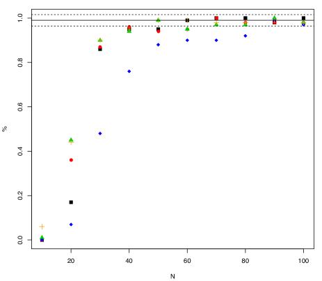
Figure 1: Proportions of the simulations where $99\%$ credibility intervals obtained with the VBEM algorithm contain the true value of the parameters, for various values of $N$ (number of vertices). $W_{11}$, black square; $W_{12}$, red circle; $U_{1}$, green triangle; $W^{*}$, blue diamond; $\alpha_{1}$, orange cross. Nominal credibility ($99\%$), solid line; binomial confidence interval, dotted lines.

5.1.2 Model selection and cluster assessment

We now aim at evaluating $IL_{osbm}$ and the quality of the recovered clusters. We first set $\epsilon=1$ and $W^{*}=-5.5$ which induces a probability $p_{inter}=g(-\epsilon+2\epsilon+W^{*})\approx 0.01$ of connection between each pair of vertices from different clusters. The values $\lambda\in\{6,4,3.5\}$ are then experimented. The corresponding probabilities $p_{intra}=g(\lambda+2\epsilon+W^{*})$ of connection between vertices of the same cluster are approximately $0.9$, $0.6$ and $0.5$. Moreover, we consider various numbers $Q_{True}$ of clusters in the set $\{2,\dots,7\}$ to generate networks, along with two scenarios depending on the type of vector $\operatorname{\boldsymbol{\alpha}}$ considered. The balanced groups correspond to equal proportions $\alpha_{1}=\dots=\alpha_{Q_{True}}=1/Q_{True}$. The unbalanced groups correspond to groups of geometric size, that is $\alpha_{q}\propto a^{q}$ and $\sum_{q=1}^{Q_{True}}\alpha_{q}=1$, for a=0.7. Considering for example $Q_{True}=7$ produces a highly unbalanced $\operatorname{\boldsymbol{\alpha}}=\{0.33,0.23,0.16,0.11,0.08,0.05,0.04\}$. Please note that the value of $a=0.7$ corresponds to an extreme case scenario which ensures, with a 0.99 chance probability, that the smallest class has at least one element. Thus, for each $Q_{True}$, each $\lambda$, and each type of vector $\operatorname{\boldsymbol{\alpha}}$, we generate $100$ networks (see an example in Figure 2) with $N=100$ vertices.

The VBEM algorithm is then applied on each network for various numbers of classes $Q\in\{2,\dots,8\}$. Note that we choose $\eta_{q}^{0}=1/2=\zeta_{q}^{0},\forall q$, $a_{0}=b_{0}=1$ and $\operatorname{\tilde{\operatorname{{\bf W}}}}^{vec}_{0}=\mathbf{0}$ for the hyperparameters. Like any optimization method, the overlapping clustering algorithm we propose depends on the initialization. Thus, for each simulated network and each number of classes $Q$, we consider $100$ initializations of $\operatorname{\boldsymbol{\tau}}$. Finally, we select the best learnt model for which the criterion $IL_{osbm}$ is maximized.

Two types of outputs are generated to present the results. The first aims at describing the accuracy of the recovered clusters. In order to compare a true $\operatorname{{\bf Z}}$ with an estimated clustering matrix $\hat{\operatorname{{\bf Z}}}$, we consider an index similar to the one proposed by Heller and Ghahramani (2007); Heller et al. (2008):

$$\sqrt{\frac{1}{N(N-1)}\sum_{i\neq j}|(\operatorname{{\bf Z}}\operatorname{{\bf Z}}^{\intercal})_{ij}-(\hat{\operatorname{{\bf Z}}}\hat{\operatorname{{\bf Z}}}^{\intercal})_{ij}|}.$$

This can be seen as a root mean square error between $\operatorname{{\bf Z}}\operatorname{{\bf Z}}^{\intercal}$ and $\hat{\operatorname{{\bf Z}}}\hat{\operatorname{{\bf Z}}}^{\intercal}$. These two $N\times N$ matrices are invariant to column permutations of $\operatorname{{\bf Z}}$ and $\hat{\operatorname{{\bf Z}}}$ and compute the number of shared clusters between each pair of vertices of a network. The better the classification, the lower this index, a null index indicating a perfect classification. The results associated to the $100$ generated networks are then summarized as boxplots.

The second type of results we generate is a confusion matrix which aims at showing the accuracy of the $IL_{osbm}$ criterion. It indicates both the real number of classes $Q_{True}$ and the number of classes selected by $IL_{osbm}$, the counts on the first diagonal corresponding to correct decisions.

The results are presented in Table 1 and Figure 3. They illustrate the relevance of $IL_{osbm}$ criterion for estimating the number of overlapping classes in networks, and show that the OSBM learnt groups are accurate. This is clearly the case when the graph is dense and the number of groups is low. The performance of the model choice criterion decreases when the density within groups decreases, and when the balance between group proportions changes (see Table 1). The same behaviour is observed concerning the quality of the overlapping clustering (see Figure 3).

Let us consider for instance the balanced case with highly connected groups. In that particular setting when $Q_{True}\in\{2,3\}$, $IL_{osbm}$ correctly estimate the number of overlapping classes of $100$ out of the $100$ networks generated. For $Q_{True}=5$, $IL_{osbm}$ still has $98$ percent accuracy. The results then slowly deteriorate for $Q_{True}\in\{6,7\}$. Indeed, as $Q_{True}$ increases while the number of vertices remains unchanged, less vertices are associated to each cluster and therefore it becomes more difficult to retrieve and distinguish the overlapping communities.

The results obtained for the unbalanced setting follow the same pattern. They are just degraded compared to balanced setting and tend to show an under-estimation of the number of groups when the connectivity within groups decreases and when the number of true groups increases. Considering for example $Q_{True}=2$ and $\lambda=3.5$ ($p_{intra}=0.5$), the estimated number of classes is accurate 98 times out of 100, but when $Q_{True}=7$ the estimated number of classes is correctly estimated only 3 times out of 100. Most of the time the model choice strategy we proposed estimates 4 groups instead of 7. This demonstrates that correctly estimating the true number of overlapping classes depends both on the intra-connectivity and the group balance.

Considering the ability of OSBM to estimate the overlapping communities, the boxplots of Figure 3 exhibits a near perfect behaviour in all settings for $Q_{True}\in\{2,3\}$. The quality of these performances degrade with a decrease of connectivity as well as a difference of balance between group proportion.

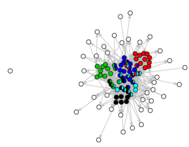
Figure 2: Example of a OSBM network with $\lambda=6$ ($p_{intra}\approx 0.9$) , $\epsilon=1$, $W^{*}=-5.5$, and $Q=5$ classes. Overlaps are represented using pies and outliers are in white.

Table 1: Confusion matrices for estimated number of classes (columns ) $Q_{IL_{osbm}}\in\{2,\dots,8\}$ versus true number of classes (rows) $Q_{True}\in\{2,\dots,7\}$ computed for balanced and unbalanced groups with three different $\lambda$ settings, $\lambda\in\{6,4,3.5\}$ corresponding respectively to three different probabilities of intra group connection $p_{intra}\approx\{0.9,0.6,0.5\}$. Notice that other parameters of simulation where set to $\epsilon=1$, $W^{*}=-5.5$

		balanced groups							unbalanced groups
		2	3	4	5	6	7	8	2	3	4	5	6	7	8
$\lambda=6$	2	$\mathbf{100}$	0	0	0	0	0	0	$\mathbf{100}$	0	0	0	0	0	0
	3	0	$\mathbf{100}$	0	0	0	0		0	$\mathbf{100}$	0	0	0	0	0
	4	0	0	$\mathbf{99}$	0	1	0	0	0	6	$\mathbf{85}$	5	3	1	0
	5	0	0	2	$\mathbf{98}$	0	0	0	0	3	34	$\mathbf{50}$	8	4	1
	6	0	0	0	8	$\mathbf{85}$	6	1	0	0	29	49	$\mathbf{15}$	6	1
	7	0	0	0	1	24	$\mathbf{56}$	19	0	0	30	50	13	$\mathbf{6}$	1
$\lambda=4$	2	$\mathbf{100}$	0	0	0	0	0	0	$\mathbf{100}$	0	0	0	0	0	0
	3	0	$\mathbf{100}$	0	0	0	0	0	0	$\mathbf{99}$	1	0	0	0	0
	4	0	0	$\mathbf{99}$	1	0	0	0	0	14	$\mathbf{68}$	9	7	2	0
	5	0	0	4	$\mathbf{79}$	14	1	2	0	18	50	$\mathbf{22}$	4	6	0
	6	0	0	1	22	$\mathbf{49}$	22	6	0	20	46	16	$\mathbf{13}$	4	1
	7	0	0	0	16	47	$\mathbf{24}$	13	0	22	56	14	5	$\mathbf{3}$	0
$\lambda=3.5$	2	$\mathbf{100}$	0	0	0	0	0	0	$\mathbf{98}$	2	0	0	0	0	0
	3	0	$\mathbf{98}$	2	0	0	0	0	1	$\mathbf{91}$	7	0	1	0	0
	4	0	0	$\mathbf{87}$	9	3	1	0	1	43	$\mathbf{32}$	16	4	1	3
	5	0	0	15	$\mathbf{44}$	26	12	3	2	34	44	$\mathbf{9}$	8	3	0
	6	0	1	11	28	$\mathbf{22}$	25	13	0	47	32	15	$\mathbf{5}$	1	0
	7	0	0	6	34	28	$\mathbf{17}$	15	2	30	46	14	5	$\mathbf{3}$	0

Figure 3: Boxplots of $\sqrt{\frac{1}{N(N-1)}\sum_{i\neq j}|(\operatorname{{\bf Z}}\operatorname{{\bf Z}}^{\intercal})_{ij}-(\hat{\operatorname{{\bf Z}}}\hat{\operatorname{{\bf Z}}}^{\intercal})_{ij}|}\$ for true number of classes $Q_{True}\in\{2,\dots,7\}$ computed for balanced and unbalanced groups with three different $\lambda$ settings, $\lambda\in\{6,4,3.5\}$ corresponding respectively to three different probabilities of intra group connection $p_{intra}\approx\{0.9,0.6,0.5\}$. Notice that other parameters of simulation where set to $\epsilon=1$, $W^{*}=-5.5$

	balanced groups	unbalanced groups
High connectivity ($\lambda=6$)
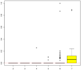
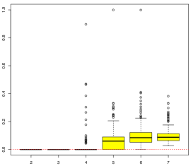
Average connectivity ($\lambda=4$)
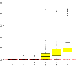
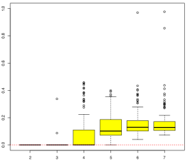
Low connectivity ($\lambda=3.5$)

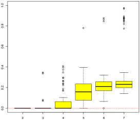
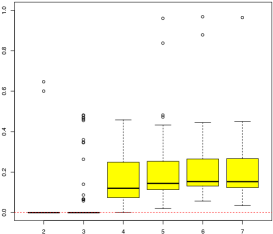
5.2 French political blogosphere

As in Latouche et al. (2011), we consider a subset of the French political blogosphere network. The network is made of 196 vertices connected by 2864 edges. It was built from a single day snapshot of political blogs automatically extracted on 14th october 2006 and manually classified by the “Observatoire Présidentiel Project” (Zanghi et al., 2008). Vertices correspond to hostnames and there is an edge between two vertices if there is a known hyperlink from one hostname to another. The five main political parties which are present in the data set are the UMP (french “republican”), liberal party (supporters of economic-liberalism), UDF (“moderate” party), PRG (“extreme left wing”) and PS (french “democrat”). In Latouche et al. (2011), we expected four political parties (UMP, liberal party, UDF, and PS) to play a key role in the network and therefore we looked for $Q=4$ clusters. The $IL_{osbm}$ model selection criterion now allows us to estimate $Q^{*}$ directly from the data, without any prior information. As we shall see, the PRG, which was discarded in the original study, also influences the topology of the network.

We run the VBEM algorithm on the data sets for $Q\in\{1,\dots,15\}$. The $IL_{osbm}$ is computed and such procedure is repeated $100$ times, for different initialization of $\operatorname{\boldsymbol{\tau}}$. Finally, we select the best learnt model for which the model selection criterion is maximized. Thus, we find $Q^{*}=12$ and a description of the corresponding clustering is given in Figure 4.

First, we notice that the first nine clusters are highly homogeneous and correspond to well known political parties. Thus, cluster 1 contains 11 vertices which are all associated to UMP. Moreover, cluster 2 contains 20 vertices all associated to the same political party. Similarly, it follows that cluster 3 and 4 correspond to the liberal party, cluster 5 to UDF, cluster 6 to PRG, and cluster 7,8, 9 to PS. These results are relevant and highlight some interesting features in the network. Indeed, clustering the vertices into $Q=4$ clusters as in Latouche et al. (2011) only gives a rough picture of the reality. In practice, the UMP, liberal party, and PS are organized into several clusters having different connection patterns. This might indicate various political affinities among the political parties. The extreme case is for the PS which was split into three clusters. Contrarily to the original study where PRG was discarded, most blogs associated to PRG were classified into the same cluster. This indicates that PRG plays a role in shaping parts of the network. Cluster 10 is also homogeneous and contains four blogs among which three correspond to blogs of political analysts.

Cluster 11 is of interest because it does not contain any single membership blog. In other words, its two blogs are both associated to other clusters. Thus, one of them was clustered in both cluster 11 and cluster 9 (PS). Its hostname is “www.parti-socialiste.fr”. The second was clustered in cluster 11 , cluster 7 (PS), and cluster 9 (PS). The corresponding hostname is “annuaire.parti-socialiste.fr”. These two blogs are the most popular blogs of PS, “www.parti-socialiste.fr” being the official website of the PS itself, while “annuaire.parti-socialiste.fr” lists all the members of PS. Interestingly, an extra component was used for the clustering, and these blogs were not just found as overlapping PS clusters, like clusters 7 and 9. This can be easily explained by the nature of these blogs. Indeed, contrarily to the PS blogs which tend to connect, as other political parties, to blogs of their own party, these blogs have extra connections to others. Blogs of other political parties tend to connect to them simply because they are a rich source of information. Finally, cluster 12 is an heterogeneous cluster, which contains blogs of different political parties, from the left wing to the right wing. Interestingly, these blogs were classified into the same cluster due to their relation ties with the world of media. In particular, we point out that three of the blogs with single memberships are blogs of political analysts. Moreover, all blogs from cluster 12 have been popular since the French presidential election in 2007, most of them being mentioned or referenced in newspapers.

We uncovered 23 overlaps in the network which are described in more detail in Table 2. As mentioned previously, we found that the liberal party and PS were organized into several clusters corresponding to sub-groups having various political affinities. Therefore, it is of no surprise to find blogs overlapping these clusters. For instance, two blogs associated with the liberal party belong to both cluster 3 (liberal) and cluster 4 (liberal). Furthermore, PS is made of 11 overlaps among which 10 are 2-membership and three-membership overlaps between clusters 7, 8, 9, and 11 all corresponding to PS clusters. One blog from PRG overlaps cluster 6 (PRG) and cluster 8 (PS). This can easily be understood since both PRG and PS are from the left wing and are known to have some relation ties. Finally, we emphasize that all political parties, except the liberal party, have overlaps with cluster 12. We recall that this cluster contains blogs with strong connection with the world of media.

In the original study in Latouche et al. (2011), with $Q=4$ clusters, 59 blogs were identified as outliers and not classified. With $Q^{*}=12$ clusters, more blogs are now classified and only 44 blogs are found as outliers (null component). These blogs have weak connection profiles compared to all the others.

overlaps	UMP	liberal	UDF	PRG	PS	analysts	others
clusters 2 (UMP)-12 (media)	$\mathbf{3}$	0	0	0	0	0	0
clusters 3 (liberal)-4 (liberal)	0	$\mathbf{2}$	0	0	0	0	0
clusters 5 (UDF)-12 (media)	0	0	$\mathbf{4}$	0	0	0	0
clusters 5 (UDF)-10 (media)	0	0	$\mathbf{1}$	0	0	0	0
clusters 6 (PRG)-8 (PS)	0	0	0	$\mathbf{1}$	0	0	0
clusters 6 (PRG)-12 (media)	0	0	0	$\mathbf{1}$	0	0	0
clusters 7 (PS)-8 (PS)	0	0	0	0	$\mathbf{2}$	0	0
clusters 8 (PS)-9 (PS)	0	0	0	0	$\mathbf{2}$	0	0
clusters 7 (PS)-9 (PS)	0	0	0	0	$\mathbf{2}$	0	0
clusters 9 (PS)-11 (PS)	0	0	0	0	$\mathbf{1}$	0	0
clusters 7 (PS)-9 (PS)-11 (PS)	0	0	0	0	$\mathbf{1}$	0	0
clusters 8 (PS)-9 (PS)-12 (media)	0	0	0	0	$\mathbf{2}$	0	0
clusters 8 (PS)-12 (media)	0	0	0	0	$\mathbf{1}$	0	0

Table 2: Description of the $23$ overlaps found when clustering the blogs into $Q=12$ clusters using OSBM. Non-zero entries are indicated in bold.

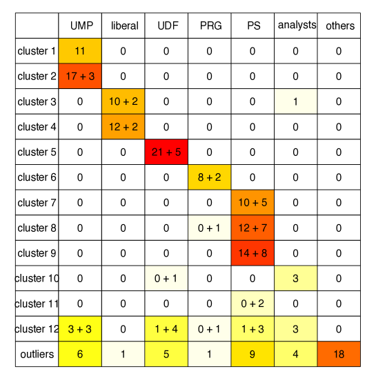
Figure 4: Classification of the blogs into $Q=12$ clusters using OSBM. The entry $(i,j)$ of the matrix describes the number of blogs associated to the $j$-th political party (column) and classified into cluster $i$ (row). Each entry distinguishes blogs which belong to a unique cluster from overlaps (single membership blogs $+$ overlaps). The last row corresponds to the null component.

6 Conclusion

In this paper, we proposed a Bayesian rewriting of the overlapping stochastic block model, which led us to an estimation algorithm and an associated model selection criterion. Introducing some conjugate prior distributions for the parameters of OSBM, we proposed a variational Bayes EM algorithm, based on global and local variational techniques. The algorithm can be used to approximate the posterior distribution over the model parameters and latent variables, given the observed data. In this framework, we derived a model selection criterion, so called $IL_{osbm}$, which is based on a non asymptotic approximation of the marginal log-likelihood. Using simulated data and a real network, we showed that $IL_{osbm}$ provides a relevant estimation of the number of overlapping clusters. In future work, we are interested in exploring parsimonious model selection in order to choose between models where some of the network structure parameters $\operatorname{{\bf U}}$, $\operatorname{{\bf V}}$, $\operatorname{{\bf W}}$ and $W^{*}$ are set to zero or not.

Appendix A: Appendix section

6.1 Lower Bound

Given a $N\times N$ positive real matrix $\operatorname{\boldsymbol{\xi}}$, a lower bound of the first lower bound can be computed:

$$\log p(\operatorname{{\bf X}})\geq{\mathcal{L}}(q)\geq{\mathcal{L}}(q;\>\operatorname{\boldsymbol{\xi}}),$$

where

$${\mathcal{L}}(q;\>\operatorname{\boldsymbol{\xi}})=\sum_{\operatorname{{\bf Z}}}\int\int\int q(\operatorname{{\bf Z}},\operatorname{\boldsymbol{\alpha}},\operatorname{\tilde{\operatorname{{\bf W}}}},\beta)\log\big{(}\frac{h(\operatorname{{\bf Z}},\operatorname{\tilde{\operatorname{{\bf W}}}},\operatorname{\boldsymbol{\xi}})p(\operatorname{{\bf Z}},\operatorname{\boldsymbol{\alpha}},\operatorname{\tilde{\operatorname{{\bf W}}}},\beta)}{q(\operatorname{{\bf Z}},\operatorname{\boldsymbol{\alpha}},\operatorname{\tilde{\operatorname{{\bf W}}}},\beta)}\big{)}d\operatorname{\boldsymbol{\alpha}}d\operatorname{\tilde{\operatorname{{\bf W}}}}d\beta,$$

and

$$\log h(\operatorname{{\bf Z}},\operatorname{\tilde{\operatorname{{\bf W}}}},\operatorname{\boldsymbol{\xi}})=\sum_{i\neq j}^{N}\left\{(X_{ij}-\frac{1}{2})a_{\operatorname{{\bf Z}}_{i},\operatorname{{\bf Z}}_{j}}-\frac{\xi_{ij}}{2}+\log g(\xi_{ij})-\lambda(\xi_{ij})(a_{\operatorname{{\bf Z}}_{i},\operatorname{{\bf Z}}_{j}}^{2}-\xi_{ij}^{2})\right\}.$$

Proof: Let us start by showing that:

$$\log p(\operatorname{{\bf X}}|\operatorname{{\bf Z}},\operatorname{\tilde{\operatorname{{\bf W}}}})\geq\log h(\operatorname{{\bf Z}},\operatorname{\tilde{\operatorname{{\bf W}}}},\operatorname{\boldsymbol{\xi}}),$$

where $\operatorname{\boldsymbol{\xi}}$ is an $N\times N$ positive real matrix. We use the bound on the log-logistic function introduced by Jaakkola and Jordan (2000):

$$\log g(x)\geq\log g(\xi)+\frac{x-\xi}{2}-\lambda(\xi)(x^{2}-\xi^{2}),\forall(x,\xi)\in\mathbb{R}\times\mathbb{R}^{+},$$ (6.1)

where $\lambda(\xi)=(g(\xi)-1/2)/(2\xi)$. Note that (6.1) is an even function and therefore we can consider only positive values of $x$ without loss of generality. Since

$$\log p(X_{ij}|\operatorname{{\bf Z}}_{i},\operatorname{{\bf Z}}_{j},\operatorname{\tilde{\operatorname{{\bf W}}}})=X_{ij}a_{\operatorname{{\bf Z}}_{i},\operatorname{{\bf Z}}_{j}}+\log g(-a_{\operatorname{{\bf Z}}_{i},\operatorname{{\bf Z}}_{j}}),$$

then

$$\log p(X_{ij}|\operatorname{{\bf Z}}_{i},\operatorname{{\bf Z}}_{j},\operatorname{\tilde{\operatorname{{\bf W}}}}) \geq X_{ij}a_{\operatorname{{\bf Z}}_{i},\operatorname{{\bf Z}}_{j}}+\log g(\xi_{ij})-\frac{a_{\operatorname{{\bf Z}}_{i},\operatorname{{\bf Z}}_{j}}+\xi_{ij}}{2}-\lambda(\xi_{ij})(a_{\operatorname{{\bf Z}}_{i},\operatorname{{\bf Z}}_{j}}^{2}-\xi_{ij}^{2})$$ (6.2)

$$=(X_{ij}-\frac{1}{2})a_{\operatorname{{\bf Z}}_{i},\operatorname{{\bf Z}}_{j}}-\frac{\xi_{ij}}{2}+\log g(\xi_{ij})-\lambda(\xi_{ij})(a_{\operatorname{{\bf Z}}_{i},\operatorname{{\bf Z}}_{j}}^{2}-\xi_{ij}^{2}).$$

Following (2.1):

$$\log p(\operatorname{{\bf X}}|\operatorname{{\bf Z}},\operatorname{\tilde{\operatorname{{\bf W}}}})=\sum_{i\neq j}^{N}\log p(\operatorname{{\bf X}}_{ij}|\operatorname{{\bf Z}}_{i},\operatorname{{\bf Z}}_{j},\operatorname{\tilde{\operatorname{{\bf W}}}}).$$

Therefore

$$\log p(\operatorname{{\bf X}}|\operatorname{{\bf Z}},\operatorname{\tilde{\operatorname{{\bf W}}}})\geq\log h(\operatorname{{\bf Z}},\operatorname{\tilde{\operatorname{{\bf W}}}},\operatorname{\boldsymbol{\xi}}).$$

We recall that the lower bound ${\mathcal{L}}(q)$ is given by:

$${\mathcal{L}}(q) =\sum_{\operatorname{{\bf Z}}}\int\int\int q(\operatorname{{\bf Z}},\operatorname{\boldsymbol{\alpha}},\operatorname{\tilde{\operatorname{{\bf W}}}},\beta)\log\left\{\frac{p(\operatorname{{\bf X}},\operatorname{{\bf Z}},\operatorname{\boldsymbol{\alpha}},\operatorname{\tilde{\operatorname{{\bf W}}}},\beta)}{q(\operatorname{{\bf Z}},\operatorname{\boldsymbol{\alpha}},\operatorname{\tilde{\operatorname{{\bf W}}}},\beta)}\right\}d\operatorname{\boldsymbol{\alpha}}d\operatorname{\tilde{\operatorname{{\bf W}}}}d\beta$$

$$=\sum_{\operatorname{{\bf Z}}}\int\int\int q(\operatorname{{\bf Z}},\operatorname{\boldsymbol{\alpha}},\operatorname{\tilde{\operatorname{{\bf W}}}},\beta)\log p(\operatorname{{\bf X}}|\operatorname{{\bf Z}},\operatorname{\tilde{\operatorname{{\bf W}}}})d\operatorname{\boldsymbol{\alpha}}d\operatorname{\tilde{\operatorname{{\bf W}}}}d\beta$$

$$\quad+\sum_{\operatorname{{\bf Z}}}\int\int\int q(\operatorname{{\bf Z}},\operatorname{\boldsymbol{\alpha}},\operatorname{\tilde{\operatorname{{\bf W}}}},\beta)\log\left\{\frac{p(\operatorname{{\bf Z}},\operatorname{\boldsymbol{\alpha}},\operatorname{\tilde{\operatorname{{\bf W}}}},\beta)}{q(\operatorname{{\bf Z}},\operatorname{\boldsymbol{\alpha}},\operatorname{\tilde{\operatorname{{\bf W}}}},\beta)}\right\}d\operatorname{\boldsymbol{\alpha}}d\operatorname{\tilde{\operatorname{{\bf W}}}}d\beta$$

$$\geq\sum_{\operatorname{{\bf Z}}}\int\int\int q(\operatorname{{\bf Z}},\operatorname{\boldsymbol{\alpha}},\operatorname{\tilde{\operatorname{{\bf W}}}},\beta)\log h(\operatorname{{\bf Z}},\operatorname{\tilde{\operatorname{{\bf W}}}},\operatorname{\boldsymbol{\xi}})d\operatorname{\boldsymbol{\alpha}}d\operatorname{\tilde{\operatorname{{\bf W}}}}d\beta$$

$$\quad+\sum_{\operatorname{{\bf Z}}}\int\int\int q(\operatorname{{\bf Z}},\operatorname{\boldsymbol{\alpha}},\operatorname{\tilde{\operatorname{{\bf W}}}},\beta)\log\left\{\frac{p(\operatorname{{\bf Z}},\operatorname{\boldsymbol{\alpha}},\operatorname{\tilde{\operatorname{{\bf W}}}},\beta)}{q(\operatorname{{\bf Z}},\operatorname{\boldsymbol{\alpha}},\operatorname{\tilde{\operatorname{{\bf W}}}},\beta)}\right\}d\operatorname{\boldsymbol{\alpha}}d\operatorname{\tilde{\operatorname{{\bf W}}}}d\beta$$

$$=\sum_{\operatorname{{\bf Z}}}\int\int\int q(\operatorname{{\bf Z}},\operatorname{\boldsymbol{\alpha}},\operatorname{\tilde{\operatorname{{\bf W}}}},\beta)\log\left\{\frac{h(\operatorname{{\bf Z}},\operatorname{\tilde{\operatorname{{\bf W}}}},\operatorname{\boldsymbol{\xi}})p(\operatorname{{\bf Z}},\operatorname{\boldsymbol{\alpha}},\operatorname{\tilde{\operatorname{{\bf W}}}},\beta)}{q(\operatorname{{\bf Z}},\operatorname{\boldsymbol{\alpha}},\operatorname{\tilde{\operatorname{{\bf W}}}},\beta)}\right\}d\operatorname{\boldsymbol{\alpha}}d\operatorname{\tilde{\operatorname{{\bf W}}}}d\beta$$

$$={\mathcal{L}}(q;\>\operatorname{\boldsymbol{\xi}}).$$

Finally

$$\log p(\operatorname{{\bf X}})\geq{\mathcal{L}}(q)\geq{\mathcal{L}}(q;\>\operatorname{\boldsymbol{\xi}}).$$

6.2 Optimization of $q(\operatorname{\boldsymbol{\alpha}})$

The optimization of the lower bound with respect to $q(\operatorname{\boldsymbol{\alpha}})$ produces a distribution with the same functional form as the prior $p(\operatorname{\boldsymbol{\alpha}})$:

$$q(\operatorname{\boldsymbol{\alpha}})=\prod_{q=1}^{Q}\operatorname{Beta}(\alpha_{q};\>\eta_{q}^{N},\zeta_{q}^{N}),$$

where

$$\eta_{q}^{N}=\eta_{q}^{0}+\sum_{i=1}^{N}\tau_{iq},$$

and

$$\zeta_{q}^{N}=\zeta_{q}^{0}+N-\sum_{i=1}^{N}\tau_{iq}.$$

Proof: According to variational Bayes, the optimal distribution $q(\operatorname{\boldsymbol{\alpha}})$ is given by:

$$\log q(\operatorname{\boldsymbol{\alpha}}) =\mathrm{E}_{\operatorname{{\bf Z}},\operatorname{\tilde{\operatorname{{\bf W}}}},\beta}[\log\big{(}h(\operatorname{{\bf Z}},\operatorname{\tilde{\operatorname{{\bf W}}}},\operatorname{\boldsymbol{\xi}})p(\operatorname{{\bf Z}},\operatorname{\boldsymbol{\alpha}},\operatorname{\tilde{\operatorname{{\bf W}}}},\beta)\big{)}]+\mathrm{const}$$ (6.3)

$$=\mathrm{E}_{\operatorname{{\bf Z}}}[\log p(\operatorname{{\bf Z}}|\operatorname{\boldsymbol{\alpha}})]+\log p(\operatorname{\boldsymbol{\alpha}})+\mathrm{const}$$

$$=\sum_{i=1}^{N}\sum_{q=1}^{Q}\left\{\tau_{iq}\log\alpha_{q}+(1-\tau_{iq})\log(1-\alpha_{q})\right\}+\sum_{q=1}^{Q}\left\{(\eta_{q}^{0}-1)\log\alpha_{q}+(\zeta_{q}^{0}-1)\log(1-\alpha_{q})\right\}$$

$$\quad+\mathrm{const}$$

$$=\sum_{q=1}^{Q}\left\{(\eta_{q}^{0}+\sum_{i=1}^{N}\tau_{iq}-1)\log\alpha_{q}+(\zeta_{q}^{0}+N-\sum_{i=1}^{N}\tau_{iq}-1)\log(1-\alpha_{q})\right\}+\mathrm{const}.$$

The functional form of (6.3) corresponds to the logarithm of a product of Beta distributions.

6.3 Optimization of $q(\operatorname{\tilde{\operatorname{{\bf W}}}})$

The optimization of the lower bound with respect to $q(\operatorname{\tilde{\operatorname{{\bf W}}}})$ produces a distribution with the same functional form as the prior $p(\operatorname{\tilde{\operatorname{{\bf W}}}})$:

$$q(\operatorname{\tilde{\operatorname{{\bf W}}}}^{vec})=\mathcal{N}(\operatorname{\tilde{\operatorname{{\bf W}}}}^{\mathrm{vec}};\>\operatorname{\tilde{\operatorname{{\bf W}}}}_{N}^{\mathrm{vec}},\operatorname{{\bf S}}_{N}),$$

with

$$\operatorname{{\bf S}}_{N}^{-1}=\frac{a_{N}}{b_{N}}\operatorname{{\bf I}}+2\sum_{i\neq j}^{N}\lambda(\xi_{ij})(\operatorname{\tilde{\operatorname{{\bf E}}}}_{j}\otimes\operatorname{\tilde{\operatorname{{\bf E}}}}_{i}),$$

and

$$\operatorname{\tilde{\operatorname{{\bf W}}}}_{N}^{\mathrm{vec}}=\operatorname{{\bf S}}_{N}\left\{\sum_{i\neq j}^{N}(X_{ij}-\frac{1}{2})\operatorname{\tilde{\operatorname{\boldsymbol{\tau}}}}_{j}\otimes\operatorname{\tilde{\operatorname{\boldsymbol{\tau}}}}_{i}\right\}.$$

Each $(Q+1)\times(Q+1)$ probability matrix $\operatorname{\tilde{\operatorname{{\bf E}}}}_{i}$ satisfies:

$$\operatorname{\tilde{\operatorname{{\bf E}}}}_{i} =\mathrm{E}_{\operatorname{{\bf Z}}_{i}}[\operatorname{\tilde{\operatorname{{\bf Z}}}}_{i}\operatorname{\tilde{\operatorname{{\bf Z}}}}_{i}^{\intercal}]$$

$$=\begin{pmatrix}\tau_{i1}&\tau_{i1}\tau_{i2}&\dots&\tau_{i1}\tau_{iQ}&\tau_{i1}\\ \tau_{i2}\tau_{i1}&\tau_{i2}&\dots&\tau_{i2}\tau_{iQ}&\tau_{i2}\\ \vdots&&&&\vdots\\ \tau_{iQ}\tau_{i1}&\tau_{iQ}\tau_{i2}&\dots&\tau_{iQ}&\tau_{iQ}\\ \tau_{i1}&\tau_{i2}&\dots&\tau_{iQ}&1\end{pmatrix}.$$

Proof: According to variational Bayes, the optimal distribution $q(\operatorname{\tilde{\operatorname{{\bf W}}}})$ is given by:

$$\log q(\operatorname{\tilde{\operatorname{{\bf W}}}}^{\mathrm{vec}}) =\mathrm{E}_{\operatorname{{\bf Z}},\operatorname{\boldsymbol{\alpha}},\beta}[\log\big{(}h(\operatorname{{\bf Z}},\operatorname{\tilde{\operatorname{{\bf W}}}},\operatorname{\boldsymbol{\xi}})p(\operatorname{{\bf Z}},\operatorname{\boldsymbol{\alpha}},\operatorname{\tilde{\operatorname{{\bf W}}}},\beta)\big{)}]+\mathrm{const}$$ (6.4)

$$=\mathrm{E}_{\operatorname{{\bf Z}}}[\log h(\operatorname{{\bf Z}},\operatorname{\tilde{\operatorname{{\bf W}}}},\operatorname{\boldsymbol{\xi}})]+\mathrm{E}_{\beta}[\log p(\operatorname{\tilde{\operatorname{{\bf W}}}}^{\mathrm{vec}}|\beta)]+\mathrm{const}$$

$$=\sum_{i\neq j}^{N}\left\{(X_{ij}-\frac{1}{2})\mathrm{E}_{\operatorname{{\bf Z}}_{i},\operatorname{{\bf Z}}_{j}}[a_{\operatorname{{\bf Z}}_{i},\operatorname{{\bf Z}}_{j}}]-\lambda(\xi_{ij})\mathrm{E}_{\operatorname{{\bf Z}}_{i},\operatorname{{\bf Z}}_{j}}[a_{\operatorname{{\bf Z}}_{i},\operatorname{{\bf Z}}_{j}}^{2}]\right\}$$

$$\>\>\>\>\>-\frac{1}{2}\mathrm{E}_{\beta}[\beta](\operatorname{\tilde{\operatorname{{\bf W}}}}^{\mathrm{vec}})^{\intercal}\operatorname{\tilde{\operatorname{{\bf W}}}}^{\mathrm{vec}}+\mathrm{const}.$$

$\mathrm{E}_{\operatorname{{\bf Z}}_{i},\operatorname{{\bf Z}}_{j}}[a_{\operatorname{{\bf Z}}_{i},\operatorname{{\bf Z}}_{j}}]$ is given by:

$$\mathrm{E}_{\operatorname{{\bf Z}}_{i},\operatorname{{\bf Z}}_{j}}[a_{\operatorname{{\bf Z}}_{i},\operatorname{{\bf Z}}_{j}}] =\mathrm{E}_{\operatorname{{\bf Z}}_{i},\operatorname{{\bf Z}}_{j}}[\operatorname{\tilde{\operatorname{{\bf Z}}}}_{i}^{\intercal}\operatorname{\tilde{\operatorname{{\bf W}}}}\operatorname{\tilde{\operatorname{{\bf Z}}}}_{j}]$$ (6.5)

$$=\operatorname{\tilde{\operatorname{\boldsymbol{\tau}}}}_{i}^{\intercal}\operatorname{\tilde{\operatorname{{\bf W}}}}\operatorname{\tilde{\operatorname{\boldsymbol{\tau}}}}_{j}$$

$$=(\operatorname{\tilde{\operatorname{\boldsymbol{\tau}}}}_{j}\otimes\operatorname{\tilde{\operatorname{\boldsymbol{\tau}}}}_{i})^{\intercal}\operatorname{\tilde{\operatorname{{\bf W}}}}^{\mathrm{vec}}$$

$$=(\operatorname{\tilde{\operatorname{{\bf W}}}}^{\mathrm{vec}})^{\intercal}(\operatorname{\tilde{\operatorname{\boldsymbol{\tau}}}}_{j}\otimes\operatorname{\tilde{\operatorname{\boldsymbol{\tau}}}}_{i}).$$

$\mathrm{E}_{\operatorname{{\bf Z}}_{i},\operatorname{{\bf Z}}_{j}}[a_{\operatorname{{\bf Z}}_{i},\operatorname{{\bf Z}}_{j}}^{2}]$ is given by:

$$\mathrm{E}_{\operatorname{{\bf Z}}_{i},\operatorname{{\bf Z}}_{j}}[a_{\operatorname{{\bf Z}}_{i},\operatorname{{\bf Z}}_{j}}^{2}] =\mathrm{E}_{\operatorname{{\bf Z}}_{i},\operatorname{{\bf Z}}_{j}}[(\operatorname{\tilde{\operatorname{{\bf Z}}}}_{i}^{\intercal}\operatorname{\tilde{\operatorname{{\bf W}}}}\operatorname{\tilde{\operatorname{{\bf Z}}}}_{j})^{2}]$$ (6.6)

$$=\mathrm{E}_{\operatorname{{\bf Z}}_{i},\operatorname{{\bf Z}}_{j}}[\big{(}(\operatorname{\tilde{\operatorname{{\bf Z}}}}_{j}\otimes\operatorname{\tilde{\operatorname{{\bf Z}}}}_{i})^{\intercal}\operatorname{\tilde{\operatorname{{\bf W}}}}^{\mathrm{vec}}\big{)}^{2}]$$

$$=\mathrm{E}_{\operatorname{{\bf Z}}_{i},\operatorname{{\bf Z}}_{j}}[(\operatorname{\tilde{\operatorname{{\bf Z}}}}_{j}\otimes\operatorname{\tilde{\operatorname{{\bf Z}}}}_{i})^{\intercal}\operatorname{\tilde{\operatorname{{\bf W}}}}^{\mathrm{vec}}(\operatorname{\tilde{\operatorname{{\bf Z}}}}_{j}\otimes\operatorname{\tilde{\operatorname{{\bf Z}}}}_{i})^{\intercal}\operatorname{\tilde{\operatorname{{\bf W}}}}^{\mathrm{vec}}]$$

$$=\mathrm{E}_{\operatorname{{\bf Z}}_{i},\operatorname{{\bf Z}}_{j}}[(\operatorname{\tilde{\operatorname{{\bf W}}}}^{\mathrm{vec}})^{\intercal}(\operatorname{\tilde{\operatorname{{\bf Z}}}}_{j}\otimes\operatorname{\tilde{\operatorname{{\bf Z}}}}_{i})(\operatorname{\tilde{\operatorname{{\bf Z}}}}_{j}\otimes\operatorname{\tilde{\operatorname{{\bf Z}}}}_{i})^{\intercal}\operatorname{\tilde{\operatorname{{\bf W}}}}^{\mathrm{vec}}]$$

$$=\mathrm{E}_{\operatorname{{\bf Z}}_{i},\operatorname{{\bf Z}}_{j}}[(\operatorname{\tilde{\operatorname{{\bf W}}}}^{\mathrm{vec}})^{\intercal}\big{(}(\operatorname{\tilde{\operatorname{{\bf Z}}}}_{j}\operatorname{\tilde{\operatorname{{\bf Z}}}}_{j}^{\intercal})\otimes(\operatorname{\tilde{\operatorname{{\bf Z}}}}_{i}\operatorname{\tilde{\operatorname{{\bf Z}}}}_{i}^{\intercal})\big{)}\operatorname{\tilde{\operatorname{{\bf W}}}}^{\mathrm{vec}}]$$

$$=(\operatorname{\tilde{\operatorname{{\bf W}}}}^{\mathrm{vec}})^{\intercal}\big{(}\operatorname{\tilde{\operatorname{{\bf E}}}}_{j}\otimes\operatorname{\tilde{\operatorname{{\bf E}}}}_{i}\big{)}\operatorname{\tilde{\operatorname{{\bf W}}}}^{\mathrm{vec}}.$$

$\mathrm{E}_{\beta}[\beta]$ is given by:

$$\mathrm{E}_{\beta}[\beta]=\frac{a_{N}}{b_{N}}.$$ (6.7)

Using (6.5), (6.6) and (6.7) in (6.4), we obtain:

$$\log q(\operatorname{\tilde{\operatorname{{\bf W}}}}^{\mathrm{vec}}) =(\operatorname{{\bf W}}^{\mathrm{vec}})^{\intercal}\left\{\sum_{i\neq j}^{N}(X_{ij}-\frac{1}{2})(\operatorname{\tilde{\operatorname{\boldsymbol{\tau}}}}_{j}\otimes\operatorname{\tilde{\operatorname{\boldsymbol{\tau}}}}_{i})\right\}$$ (6.8)

$$\>\>\>\>\>-\frac{1}{2}(\operatorname{\tilde{\operatorname{{\bf W}}}}^{\mathrm{vec}})^{\intercal}\left\{\frac{a_{N}}{b_{N}}\operatorname{{\bf I}}+2\sum_{i\neq j}^{N}\lambda(\xi_{ij})\big{(}\operatorname{\tilde{\operatorname{{\bf E}}}}_{j}\otimes\operatorname{\tilde{\operatorname{{\bf E}}}}_{i}\big{)}\right\}\operatorname{\tilde{\operatorname{{\bf W}}}}^{\mathrm{vec}}+\mathrm{const}.$$

The functional form of (6.8) corresponds to the logarithm of a Gaussian distribution with mean $\operatorname{\tilde{\operatorname{{\bf W}}}}^{\mathrm{vec}}_{N}$ and covariance matrix $\operatorname{{\bf S}}_{N}$.

6.4 Optimization of $q(\beta)$

The optimization of the lower bound with respect to $q(\beta)$ produces a distribution with the same functional form as the prior $p(\beta)$:

$$q(\beta)=\operatorname{Gam}(\beta;\>a_{N},b_{N}),$$

where

$$a_{N}=a_{0}+\frac{(Q+1)^{2}}{2},$$

and

$$b_{N}=b_{0}+\frac{1}{2}\mathrm{Tr}(S_{N})+\frac{1}{2}(\operatorname{\tilde{\operatorname{{\bf W}}}}_{N}^{\mathrm{vec}})^{\intercal}\operatorname{\tilde{\operatorname{{\bf W}}}}_{N}^{\mathrm{vec}}.$$

Proof: According to variational Bayes, the optimal distribution $q(\beta)$ is given by:

$$\log q(\beta) =\mathrm{E}_{\operatorname{{\bf Z}},\operatorname{\boldsymbol{\alpha}},\operatorname{\tilde{\operatorname{{\bf W}}}}}[\log\big{(}h(\operatorname{{\bf Z}},\operatorname{\tilde{\operatorname{{\bf W}}}},\operatorname{\boldsymbol{\xi}})p(\operatorname{{\bf Z}},\operatorname{\boldsymbol{\alpha}},\operatorname{\tilde{\operatorname{{\bf W}}}},\beta)\big{)}]+\mathrm{const}$$ (6.9)

$$=\mathrm{E}_{\operatorname{\tilde{\operatorname{{\bf W}}}}}[\log p(\operatorname{\tilde{\operatorname{{\bf W}}}}|\beta)]+\log p(\beta)+\mathrm{const}$$

$$=-\frac{1}{2}\log|\frac{\operatorname{{\bf I}}}{\beta}|-\frac{\beta}{2}\mathrm{E}_{\operatorname{\tilde{\operatorname{{\bf W}}}}}[(\operatorname{\tilde{\operatorname{{\bf W}}}}^{\mathrm{vec}})^{\intercal}\operatorname{\tilde{\operatorname{{\bf W}}}}^{\mathrm{vec}}]+(a_{0}-1)\log\beta-b_{0}\beta+\mathrm{const}$$

$$=\big{(}a_{0}+\frac{(Q+1)^{2}}{2}-1\big{)}\log\beta-\beta\Big{(}b_{0}+\frac{1}{2}\mathrm{Tr}(S_{N})+\frac{1}{2}(\operatorname{\tilde{\operatorname{{\bf W}}}}_{N}^{\mathrm{vec}})^{\intercal}\operatorname{\tilde{\operatorname{{\bf W}}}}_{N}^{\mathrm{vec}}\Big{)}+\mathrm{const}.$$

The functional form of (6.9) corresponds to the logarithm of a Gamma distribution.

6.5 Optimization of $q(Z_{iq})$

The optimization of the lower bound with respect to $q(Z_{iq})$ produces a distribution with the same functional form as the prior $p(Z_{iq}|\operatorname{\boldsymbol{\alpha}})$:

$$q(Z_{iq})=\mathcal{B}(Z_{iq};\>\tau_{iq}),$$

where

$$\tau_{iq} =g\bigg{\{}\psi(\eta_{q}^{N})-\psi(\zeta_{q}^{N})+\sum_{j\neq i}^{N}(X_{ij}-\frac{1}{2})\operatorname{\tilde{\operatorname{\boldsymbol{\tau}}}}_{j}^{\intercal}(\operatorname{\tilde{\operatorname{{\bf W}}}}_{N}^{\intercal})_{\cdot q}+\sum_{j\neq i}^{N}(X_{ji}-\frac{1}{2})\operatorname{\tilde{\operatorname{\boldsymbol{\tau}}}}_{j}^{\intercal}(\operatorname{\tilde{\operatorname{{\bf W}}}}_{N})_{\cdot q}$$

$$\>\>\>\>\>-\mathrm{Tr}\Big{(}\big{(}\operatorname{\boldsymbol{\Sigma}}_{qq}^{{}^{\prime}}+2\sum_{l\neq q}^{Q+1}\tilde{\tau}_{il}\operatorname{\boldsymbol{\Sigma}}_{ql}^{{}^{\prime}}\big{)}\big{(}\sum_{j\neq i}^{N}\lambda(\xi_{ij})\operatorname{\tilde{\operatorname{{\bf E}}}}_{j}\big{)}+\big{(}\operatorname{\boldsymbol{\Sigma}}_{qq}+2\sum_{l\neq q}^{Q+1}\tilde{\tau}_{il}\operatorname{\boldsymbol{\Sigma}}_{ql}\big{)}\big{(}\sum_{j\neq i}^{N}\lambda(\xi_{ji})\operatorname{\tilde{\operatorname{{\bf E}}}}_{j}\big{)}\Big{)}\bigg{\}},$$

and $\operatorname{\boldsymbol{\Sigma}}_{ql}=\mathrm{E}_{\operatorname{\tilde{\operatorname{{\bf W}}}}_{q},\operatorname{\tilde{\operatorname{{\bf W}}}}_{l}}[\operatorname{\tilde{\operatorname{{\bf W}}}}_{\cdot q}\operatorname{\tilde{\operatorname{{\bf W}}}}_{\cdot l}^{\intercal}]$, $\operatorname{\boldsymbol{\Sigma}}_{ql}^{{}^{\prime}}=\mathrm{E}_{\operatorname{\tilde{\operatorname{{\bf W}}}}_{q\cdot},\operatorname{\tilde{\operatorname{{\bf W}}}}_{l\cdot}}[\operatorname{\tilde{\operatorname{{\bf W}}}}_{q\cdot}^{\intercal}\operatorname{\tilde{\operatorname{{\bf W}}}}_{l\cdot}]$.

Proof: According to variational Bayes, the optimal distribution $q(Z_{iq})$ is given by:

$$\log q(Z_{bc})=\mathrm{E}_{\operatorname{{\bf Z}}^{\backslash bc},\operatorname{\boldsymbol{\alpha}},\operatorname{\tilde{\operatorname{{\bf W}}}},\beta}[\log\big{(}h(\operatorname{{\bf Z}},\operatorname{\tilde{\operatorname{{\bf W}}}},\operatorname{\boldsymbol{\xi}})p(\operatorname{{\bf Z}},\operatorname{\boldsymbol{\alpha}},\operatorname{\tilde{\operatorname{{\bf W}}}},\beta)\big{)}]+\mathrm{const},$$

where $\operatorname{{\bf Z}}^{\backslash bc}$ is the set of all class memberships except $Z_{bc}$.

$$\log q(Z_{bc})=\mathrm{E}_{\operatorname{{\bf Z}}^{\backslash bc},\operatorname{\tilde{\operatorname{{\bf W}}}}}[\log h(\operatorname{{\bf Z}},\operatorname{\tilde{\operatorname{{\bf W}}}},\operatorname{\boldsymbol{\xi}})]+\mathrm{E}_{\operatorname{{\bf Z}}^{\backslash bc},\operatorname{\boldsymbol{\alpha}}}[\log p(\operatorname{{\bf Z}}|\operatorname{\boldsymbol{\alpha}})]+\mathrm{const}.$$

$\mathrm{E}_{\operatorname{{\bf Z}}^{\backslash bc},\operatorname{\boldsymbol{\alpha}}}[\log p(\operatorname{{\bf Z}}|\operatorname{\boldsymbol{\alpha}})]$ is given by:

$$\mathrm{E}_{\operatorname{{\bf Z}}^{\backslash bc},\operatorname{\boldsymbol{\alpha}}}[\log p(\operatorname{{\bf Z}}|\operatorname{\boldsymbol{\alpha}})] =Z_{bc}\mathrm{E}_{\alpha_{c}}[\log\alpha_{c}]+(1-Z_{bc})\mathrm{E}_{\alpha_{c}}[\log(1-\alpha_{c})]+\mathrm{const}$$

$$=Z_{bc}\big{(}\psi(\eta_{c}^{N})-\psi(\eta_{c}^{N}+\zeta_{c}^{N})\big{)}+(1-Z_{bc})\big{(}\psi(\zeta_{c}^{N})-\psi(\eta_{c}^{N}+\zeta_{c}^{N})\big{)}+\mathrm{const}$$

$$=Z_{bc}\big{(}\psi(\eta_{c}^{N})-\psi(\zeta_{c}^{N})\big{)}+\mathrm{const},$$

where $\psi(\cdot)$ is the digamma function (the logarithmic derivative of the gamma function $\Gamma(\cdot)$ which appears in the normalizing constants of the Beta distributions).

$$\mathrm{E}_{\operatorname{{\bf Z}}^{\backslash bc},\operatorname{\tilde{\operatorname{{\bf W}}}}}[\log h(\operatorname{{\bf Z}},\operatorname{\tilde{\operatorname{{\bf W}}}},\operatorname{\boldsymbol{\xi}})] =\sum_{i\neq j}^{N}\left\{(X_{ij}-\frac{1}{2})\mathrm{E}_{\operatorname{{\bf Z}}^{\backslash bc},\operatorname{\tilde{\operatorname{{\bf W}}}}}[a_{\operatorname{{\bf Z}}_{i},\operatorname{{\bf Z}}_{j}}]-\lambda(\xi_{ij})\mathrm{E}_{\operatorname{{\bf Z}}^{\backslash bc},\operatorname{\tilde{\operatorname{{\bf W}}}}}[a_{\operatorname{{\bf Z}}_{i},\operatorname{{\bf Z}}_{j}}^{2}]\right\}+\mathrm{const}$$

$$=\sum_{j\neq b}^{N}\left\{(X_{bj}-\frac{1}{2})\mathrm{E}_{\operatorname{{\bf Z}}_{b}^{\backslash c},\operatorname{{\bf Z}}_{j},\operatorname{\tilde{\operatorname{{\bf W}}}}}[a_{\operatorname{{\bf Z}}_{b},\operatorname{{\bf Z}}_{j}}]-\lambda(\xi_{bj})\mathrm{E}_{\operatorname{{\bf Z}}_{b}^{\backslash c},\operatorname{{\bf Z}}_{j},\operatorname{\tilde{\operatorname{{\bf W}}}}}[a_{\operatorname{{\bf Z}}_{b},\operatorname{{\bf Z}}_{j}}^{2}]\right\}$$

$$\>\>\>\>\>+\sum_{i\neq b}^{N}\left\{(X_{ib}-\frac{1}{2})\mathrm{E}_{\operatorname{{\bf Z}}_{b}^{\backslash c},\operatorname{{\bf Z}}_{i},\operatorname{\tilde{\operatorname{{\bf W}}}}}[a_{\operatorname{{\bf Z}}_{i},\operatorname{{\bf Z}}_{b}}]-\lambda(\xi_{ib})\mathrm{E}_{\operatorname{{\bf Z}}_{b}^{\backslash c},\operatorname{{\bf Z}}_{i},\operatorname{\tilde{\operatorname{{\bf W}}}}}[a_{\operatorname{{\bf Z}}_{i},\operatorname{{\bf Z}}_{b}}^{2}]\right\}+\mathrm{const}$$

$$=\sum_{j\neq b}^{N}\Big{\{}(X_{bj}-\frac{1}{2})\mathrm{E}_{\operatorname{{\bf Z}}_{b}^{\backslash c},\operatorname{{\bf Z}}_{j},\operatorname{\tilde{\operatorname{{\bf W}}}}}[a_{\operatorname{{\bf Z}}_{b},\operatorname{{\bf Z}}_{j}}]+(X_{jb}-\frac{1}{2})\mathrm{E}_{\operatorname{{\bf Z}}_{b}^{\backslash c},\operatorname{{\bf Z}}_{j},\operatorname{\tilde{\operatorname{{\bf W}}}}}[a_{\operatorname{{\bf Z}}_{j},\operatorname{{\bf Z}}_{b}}]$$

$$\>\>\>\>\>-\lambda(\xi_{bj})\mathrm{E}_{\operatorname{{\bf Z}}_{b}^{\backslash c},\operatorname{{\bf Z}}_{j},\operatorname{\tilde{\operatorname{{\bf W}}}}}[a_{\operatorname{{\bf Z}}_{b},\operatorname{{\bf Z}}_{j}}^{2}]-\lambda(\xi_{jb})\mathrm{E}_{\operatorname{{\bf Z}}_{b}^{\backslash c},\operatorname{{\bf Z}}_{j},\operatorname{\tilde{\operatorname{{\bf W}}}}}[a_{\operatorname{{\bf Z}}_{j},\operatorname{{\bf Z}}_{b}}^{2}]\Big{\}}+\mathrm{const}.$$

$$\mathrm{E}_{\operatorname{{\bf Z}}_{b}^{\backslash c},\operatorname{{\bf Z}}_{j},\operatorname{\tilde{\operatorname{{\bf W}}}}}[a_{\operatorname{{\bf Z}}_{b},\operatorname{{\bf Z}}_{j}}] =\mathrm{E}_{\operatorname{{\bf Z}}_{b}^{\backslash c},\operatorname{{\bf Z}}_{j},\operatorname{\tilde{\operatorname{{\bf W}}}}}[\sum_{q,l}^{Q+1}\operatorname{\tilde{Z}}_{bq}\operatorname{\tilde{W}}_{ql}\operatorname{\tilde{Z}}_{jl}]$$

$$=Z_{bc}\sum_{l=1}^{Q+1}\mathrm{E}_{\operatorname{\tilde{W}}_{cl}}[\operatorname{\tilde{W}}_{cl}]\tilde{\tau}_{jl}+\mathrm{const}$$

$$=Z_{bc}\operatorname{\tilde{\operatorname{\boldsymbol{\tau}}}}_{j}^{\intercal}(\operatorname{\tilde{\operatorname{{\bf W}}}}_{N}^{\intercal})_{\cdot c}+\mathrm{const}.$$

$$\mathrm{E}_{\operatorname{{\bf Z}}_{b}^{\backslash c},\operatorname{{\bf Z}}_{j},\operatorname{\tilde{\operatorname{{\bf W}}}}}[a_{\operatorname{{\bf Z}}_{j},\operatorname{{\bf Z}}_{b}}] =\mathrm{E}_{\operatorname{{\bf Z}}_{b}^{\backslash c},\operatorname{{\bf Z}}_{j},\operatorname{\tilde{\operatorname{{\bf W}}}}}[\sum_{q,l}^{Q+1}\operatorname{\tilde{Z}}_{jq}\operatorname{\tilde{W}}_{ql}\operatorname{\tilde{Z}}_{bl}]$$

$$=Z_{bc}\sum_{l=1}^{Q+1}\mathrm{E}_{\operatorname{\tilde{W}}_{lc}}[\operatorname{\tilde{W}}_{lc}]\tilde{\tau}_{jl}+\mathrm{const}$$

$$=Z_{bc}\operatorname{\tilde{\operatorname{\boldsymbol{\tau}}}}_{j}^{\intercal}(\operatorname{\tilde{\operatorname{{\bf W}}}}_{N})_{\cdot c}+\mathrm{const}.$$

$$\mathrm{E}_{\operatorname{{\bf Z}}_{b}^{\backslash c},\operatorname{{\bf Z}}_{j},\operatorname{\tilde{\operatorname{{\bf W}}}}}[a_{\operatorname{{\bf Z}}_{j},\operatorname{{\bf Z}}_{b}}^{2}] =\mathrm{E}_{\operatorname{{\bf Z}}_{b}^{\backslash c},\operatorname{{\bf Z}}_{j},\operatorname{\tilde{\operatorname{{\bf W}}}}}[\big{(}\sum_{q,l}^{Q+1}\operatorname{\tilde{Z}}_{jq}\operatorname{\tilde{W}}_{ql}\operatorname{\tilde{Z}}_{bl}\big{)}\big{(}\sum_{q,l}^{Q+1}\operatorname{\tilde{Z}}_{jq}\operatorname{\tilde{W}}_{ql}\operatorname{\tilde{Z}}_{bl}\big{)}]$$

$$=\mathrm{E}_{\operatorname{{\bf Z}}_{b}^{\backslash c},\operatorname{{\bf Z}}_{j},\operatorname{\tilde{\operatorname{{\bf W}}}}}[\sum_{q,q^{{}^{\prime}},l,l^{{}^{\prime}}}^{Q+1}\operatorname{\tilde{Z}}_{bl}\operatorname{\tilde{Z}}_{bl^{{}^{\prime}}}\operatorname{\tilde{Z}}_{jq}\operatorname{\tilde{W}}_{ql}\operatorname{\tilde{W}}_{q^{{}^{\prime}}l^{{}^{\prime}}}\operatorname{\tilde{Z}}_{jq^{{}^{\prime}}}]$$

$$=\mathrm{E}_{\operatorname{{\bf Z}}_{b}^{\backslash c},\operatorname{{\bf Z}}_{j},\operatorname{\tilde{\operatorname{{\bf W}}}}}[Z_{bc}\sum_{q,q^{{}^{\prime}}}^{Q+1}\operatorname{\tilde{Z}}_{jq}\operatorname{\tilde{W}}_{qc}\operatorname{\tilde{W}}_{q^{{}^{\prime}}c}\operatorname{\tilde{Z}}_{jq^{{}^{\prime}}}+2Z_{bc}\sum_{q,q^{{}^{\prime}},l\neq c}^{Q+1}\operatorname{\tilde{Z}}_{bl}\operatorname{\tilde{Z}}_{jq}\operatorname{\tilde{W}}_{qc}\operatorname{\tilde{W}}_{q^{{}^{\prime}}l}\operatorname{\tilde{Z}}_{jq^{{}^{\prime}}}]+\mathrm{const}$$

$$=Z_{bc}\left\{\mathrm{E}_{\operatorname{{\bf Z}}_{j},\operatorname{\tilde{\operatorname{{\bf W}}}}_{\cdot c}}[\operatorname{\tilde{\operatorname{{\bf W}}}}_{\cdot c}^{\intercal}\operatorname{\tilde{\operatorname{{\bf Z}}}}_{j}\operatorname{\tilde{\operatorname{{\bf Z}}}}_{j}^{\intercal}\operatorname{\tilde{\operatorname{{\bf W}}}}_{\cdot c}]+2\sum_{l\neq c}^{Q+1}\tilde{\tau}_{bl}\mathrm{E}_{\operatorname{{\bf Z}}_{j},\operatorname{\tilde{\operatorname{{\bf W}}}}_{\cdot c},\operatorname{\tilde{\operatorname{{\bf W}}}}_{\cdot l}}[\operatorname{\tilde{\operatorname{{\bf W}}}}_{\cdot c}^{\intercal}\operatorname{\tilde{\operatorname{{\bf Z}}}}_{j}\operatorname{\tilde{\operatorname{{\bf Z}}}}_{j}^{\intercal}\operatorname{\tilde{\operatorname{{\bf W}}}}_{\cdot l}]\right\}+\mathrm{const}$$

$$=Z_{bc}\left\{\mathrm{E}_{\operatorname{\tilde{\operatorname{{\bf W}}}}_{\cdot,c}}[\operatorname{\tilde{\operatorname{{\bf W}}}}_{\cdot c}^{\intercal}\operatorname{\tilde{\operatorname{{\bf E}}}}_{j}\operatorname{\tilde{\operatorname{{\bf W}}}}_{\cdot c}]+2\sum_{l\neq c}^{Q+1}\tilde{\tau}_{bl}\mathrm{E}_{\operatorname{\tilde{\operatorname{{\bf W}}}}_{\cdot c},\operatorname{\tilde{\operatorname{{\bf W}}}}_{\cdot l}}[\operatorname{\tilde{\operatorname{{\bf W}}}}_{\cdot c}^{\intercal}\operatorname{\tilde{\operatorname{{\bf E}}}}_{j}\operatorname{\tilde{\operatorname{{\bf W}}}}_{\cdot l}]\right\}+\mathrm{const}$$

$$=Z_{bc}\left\{\mathrm{E}_{\operatorname{\tilde{\operatorname{{\bf W}}}}_{\cdot c}}[(\operatorname{\tilde{\operatorname{{\bf W}}}}_{\cdot c}\otimes\operatorname{\tilde{\operatorname{{\bf W}}}}_{\cdot c})^{\intercal}]\operatorname{\tilde{\operatorname{{\bf E}}}}_{j}^{\mathrm{vec}}+2\sum_{l\neq c}^{Q+1}\tilde{\tau}_{bl}\mathrm{E}_{\operatorname{\tilde{\operatorname{{\bf W}}}}_{\cdot c},\operatorname{\tilde{\operatorname{{\bf W}}}}_{\cdot l}}[(\operatorname{\tilde{\operatorname{{\bf W}}}}_{\cdot l}\otimes\operatorname{\tilde{\operatorname{{\bf W}}}}_{\cdot c})^{\intercal}]\operatorname{\tilde{\operatorname{{\bf E}}}}_{j}^{\mathrm{vec}}\right\}+\mathrm{const}$$

$$=Z_{bc}\left\{\mathrm{E}_{\operatorname{\tilde{\operatorname{{\bf W}}}}_{\cdot c}}[((\operatorname{\tilde{\operatorname{{\bf W}}}}_{\cdot c}\operatorname{\tilde{\operatorname{{\bf W}}}}_{\cdot c}^{\intercal})^{\mathrm{vec}})^{\intercal}]\operatorname{\tilde{\operatorname{{\bf E}}}}_{j}^{\mathrm{vec}}+2\sum_{l\neq c}^{Q+1}\tilde{\tau}_{bl}\mathrm{E}_{\operatorname{\tilde{\operatorname{{\bf W}}}}_{\cdot c},\operatorname{\tilde{\operatorname{{\bf W}}}}_{\cdot l}}[((\operatorname{\tilde{\operatorname{{\bf W}}}}_{\cdot c}\operatorname{\tilde{\operatorname{{\bf W}}}}_{\cdot l}^{\intercal})^{\mathrm{vec}})^{\intercal}]\operatorname{\tilde{\operatorname{{\bf E}}}}_{j}^{\mathrm{vec}}\right\}+\mathrm{const}$$

$$=Z_{bc}\left\{(\operatorname{\boldsymbol{\Sigma}}_{cc}^{\mathrm{vec}})^{\intercal}\operatorname{\tilde{\operatorname{{\bf E}}}}_{j}^{\mathrm{vec}}+2\sum_{l\neq c}^{Q+1}\tilde{\tau}_{bl}(\operatorname{\boldsymbol{\Sigma}}_{cl}^{\mathrm{vec}})^{\intercal}\operatorname{\tilde{\operatorname{{\bf E}}}}_{j}^{\mathrm{vec}}\right\}+\mathrm{const}$$

$$=Z_{bc}\mathrm{Tr}\Big{(}\big{(}\operatorname{\boldsymbol{\Sigma}}_{cc}+2\sum_{l\neq c}^{Q+1}\tilde{\tau}_{bl}\operatorname{\boldsymbol{\Sigma}}_{cl}\big{)}\operatorname{\tilde{\operatorname{{\bf E}}}}_{j}\Big{)}+\mathrm{const},$$

where $\operatorname{\boldsymbol{\Sigma}}_{ql}=\mathrm{E}_{\operatorname{\tilde{\operatorname{{\bf W}}}}_{q},\operatorname{\tilde{\operatorname{{\bf W}}}}_{l}}[\operatorname{\tilde{\operatorname{{\bf W}}}}_{\cdot q}\operatorname{\tilde{\operatorname{{\bf W}}}}_{\cdot l}^{\intercal}]$. Similarly, we have:

$$\mathrm{E}_{\operatorname{{\bf Z}}_{b}^{\backslash c},\operatorname{{\bf Z}}_{j},\operatorname{\tilde{\operatorname{{\bf W}}}}}[a_{\operatorname{{\bf Z}}_{b},\operatorname{{\bf Z}}_{j}}^{2}]=Z_{bc}\mathrm{Tr}\Big{(}\big{(}\operatorname{\boldsymbol{\Sigma}}_{cc}^{{}^{\prime}}+2\sum_{l\neq c}^{Q+1}\tilde{\tau}_{bl}\operatorname{\boldsymbol{\Sigma}}_{cl}^{{}^{\prime}}\big{)}\operatorname{\tilde{\operatorname{{\bf E}}}}_{j}\Big{)}+\mathrm{const},$$

where $\operatorname{\boldsymbol{\Sigma}}_{ql}^{{}^{\prime}}=\mathrm{E}_{\operatorname{\tilde{\operatorname{{\bf W}}}}_{q\cdot},\operatorname{\tilde{\operatorname{{\bf W}}}}_{l\cdot}}[\operatorname{\tilde{\operatorname{{\bf W}}}}_{q\cdot}^{\intercal}\operatorname{\tilde{\operatorname{{\bf W}}}}_{l\cdot}]$. Finally, we obtain:

$$\log q(Z_{bc}) =Z_{bc}\bigg{\{}\psi(\eta_{c}^{N})-\psi(\zeta_{c}^{N})+\sum_{j\neq b}^{N}(X_{bj}-\frac{1}{2})\operatorname{\tilde{\operatorname{\boldsymbol{\tau}}}}_{j}^{\intercal}(\operatorname{\tilde{\operatorname{{\bf W}}}}_{N}^{\intercal})_{\cdot c}+\sum_{j\neq b}^{N}(X_{jb}-\frac{1}{2})\operatorname{\tilde{\operatorname{\boldsymbol{\tau}}}}_{j}^{\intercal}(\operatorname{\tilde{\operatorname{{\bf W}}}}_{N})_{\cdot c}$$ (6.10)

$$\>\>\>\>\>-\mathrm{Tr}\Big{(}\big{(}\operatorname{\boldsymbol{\Sigma}}_{cc}^{{}^{\prime}}+2\sum_{l\neq c}^{Q+1}\tilde{\tau}_{bl}\operatorname{\boldsymbol{\Sigma}}_{cl}^{{}^{\prime}}\big{)}\big{(}\sum_{j\neq b}^{N}\lambda(\xi_{bj})\operatorname{\tilde{\operatorname{{\bf E}}}}_{j}\big{)}+\big{(}\operatorname{\boldsymbol{\Sigma}}_{cc}+2\sum_{l\neq c}^{Q+1}\tilde{\tau}_{bl}\operatorname{\boldsymbol{\Sigma}}_{cl}\big{)}\big{(}\sum_{j\neq b}^{N}\lambda(\xi_{jb})\operatorname{\tilde{\operatorname{{\bf E}}}}_{j}\big{)}\Big{)}\bigg{\}}$$

$$\quad+\mathrm{const}.$$

The functional form of (6.10) corresponds to the logarithm of a Bernoulli distribution with parameter $\tau_{bc}$. Indeed:

$$\log\mathcal{B}(Z_{bc};\>\tau_{bc}) =Z_{bc}\log\tau_{bc}+(1-Z_{bc})\log(1-\tau_{bc})$$

$$=Z_{bc}\log(\frac{\tau_{bc}}{1-\tau_{bc}})+\mathrm{const}.$$

If we denote $p=\log\big{(}\tau_{bc}/(1-\tau_{bc})\big{)}$, then $\tau_{bc}=g(p)$.

6.6 Optimization of $\operatorname{\boldsymbol{\xi}}$

Setting the partial derivative of the lower bound with respect to $\xi_{ij}$, to zero, leads to an estimate $\hat{\xi_{ij}}$ of $\xi_{ij}$:

$$\hat{\xi}_{ij}=\sqrt{\mathrm{Tr}\Big{(}\big{(}\operatorname{{\bf S}}_{N}+\operatorname{\tilde{\operatorname{{\bf W}}}}_{N}^{\mathrm{vec}}(\operatorname{\tilde{\operatorname{{\bf W}}}}_{N}^{\mathrm{vec}})^{\intercal}\big{)}(\operatorname{\tilde{\operatorname{{\bf E}}}}_{j}\otimes\operatorname{\tilde{\operatorname{{\bf E}}}}_{i})\Big{)}}.$$

Proof: The partial derivative of the lower bound with respect to $\xi_{ij}$ is given by:

$$\frac{\partial{\mathcal{L}}}{\partial\xi_{ij}}(q;\>\operatorname{\boldsymbol{\xi}})=-\frac{1}{2}+g(-\xi_{ij})-\lambda^{{}^{\prime}}(\xi_{ij})\big{(}\mathrm{E}_{\operatorname{{\bf Z}}_{i},\operatorname{{\bf Z}}_{j},\operatorname{\tilde{\operatorname{{\bf W}}}}}[a_{\operatorname{{\bf Z}}_{i},\operatorname{{\bf Z}}_{j}}^{2}]-\xi_{ij}^{2}\big{)}+2\xi_{ij}\lambda(\xi_{ij}).$$

According to (6.6),

$$\mathrm{E}_{\operatorname{{\bf Z}}_{i},\operatorname{{\bf Z}}_{j}}[a_{\operatorname{{\bf Z}}_{i},\operatorname{{\bf Z}}_{j}}^{2}]=(\operatorname{\tilde{\operatorname{{\bf W}}}}^{\mathrm{vec}})^{\intercal}\big{(}\operatorname{\tilde{\operatorname{{\bf E}}}}_{j}\otimes\operatorname{\tilde{\operatorname{{\bf E}}}}_{i}\big{)}\operatorname{\tilde{\operatorname{{\bf W}}}}^{\mathrm{vec}},$$

therefore

$$\mathrm{E}_{\operatorname{{\bf Z}}_{i},\operatorname{{\bf Z}}_{j},\operatorname{\tilde{\operatorname{{\bf W}}}}}[a_{\operatorname{{\bf Z}}_{i},\operatorname{{\bf Z}}_{j}}^{2}] =\mathrm{E}_{\operatorname{\tilde{\operatorname{{\bf W}}}}}[(\operatorname{\tilde{\operatorname{{\bf W}}}}^{\mathrm{vec}})^{\intercal}(\operatorname{\tilde{\operatorname{{\bf E}}}}_{j}\otimes\operatorname{\tilde{\operatorname{{\bf E}}}}_{i})\operatorname{\tilde{\operatorname{{\bf W}}}}^{\mathrm{vec}}]$$ (6.11)

$$=\mathrm{E}_{\operatorname{\tilde{\operatorname{{\bf W}}}}}\Big{[}[\mathrm{Tr}\Big{(}\operatorname{\tilde{\operatorname{{\bf W}}}}^{\mathrm{vec}}(\operatorname{\tilde{\operatorname{{\bf W}}}}^{\mathrm{vec}})^{\intercal}(\operatorname{\tilde{\operatorname{{\bf E}}}}_{j}\otimes\operatorname{\tilde{\operatorname{{\bf E}}}}_{i})\Big{)}\Big{]}$$

$$=\mathrm{Tr}\Big{(}\mathrm{E}_{\operatorname{\tilde{\operatorname{{\bf W}}}}}\big{[}\operatorname{\tilde{\operatorname{{\bf W}}}}^{\mathrm{vec}}(\operatorname{\tilde{\operatorname{{\bf W}}}}^{\mathrm{vec}})^{\intercal}\big{]}(\operatorname{\tilde{\operatorname{{\bf E}}}}_{j}\otimes\operatorname{\tilde{\operatorname{{\bf E}}}}_{i})\Big{)}$$

$$=\mathrm{Tr}\Big{(}\big{(}\operatorname{{\bf S}}_{N}+\operatorname{\tilde{\operatorname{{\bf W}}}}_{N}^{\mathrm{vec}}(\operatorname{\tilde{\operatorname{{\bf W}}}}_{N}^{\mathrm{vec}})^{\intercal}\big{)}(\operatorname{\tilde{\operatorname{{\bf E}}}}_{j}\otimes\operatorname{\tilde{\operatorname{{\bf E}}}}_{i})\Big{)}.$$

Moreover $(\log g)^{{}^{\prime}}(\xi_{ij})=g(-\xi_{ij})$ and $g(\xi_{j})+g(-\xi_{ij})=1$. We obtain:

$$\frac{\partial{\mathcal{L}}}{\partial\xi_{ij}}(q;\>\operatorname{\boldsymbol{\xi}})=-\lambda^{{}^{\prime}}(\xi_{ij})\left\{\mathrm{Tr}\Big{(}\big{(}\operatorname{{\bf S}}_{N}+\operatorname{\tilde{\operatorname{{\bf W}}}}_{N}^{\mathrm{vec}}(\operatorname{\tilde{\operatorname{{\bf W}}}}_{N}^{\mathrm{vec}})^{\intercal}\big{)}(\operatorname{\tilde{\operatorname{{\bf E}}}}_{j}\otimes\operatorname{\tilde{\operatorname{{\bf E}}}}_{i})\Big{)}-\xi_{ij}^{2}\right\}.$$

Finally, $\lambda(\xi_{ij})$ is a strictly decreasing function for positive values of $\xi_{ij}$. Thus, $\lambda^{{}^{\prime}}(\xi_{ij})\neq 0$ and if we set the derivative of (6.6) to zero, it leads to:

$$\xi_{ij}^{2}=\mathrm{Tr}\Big{(}\big{(}\operatorname{{\bf S}}_{N}+\operatorname{\tilde{\operatorname{{\bf W}}}}_{N}^{\mathrm{vec}}(\operatorname{\tilde{\operatorname{{\bf W}}}}_{N}^{\mathrm{vec}})^{\intercal}\big{)}(\operatorname{\tilde{\operatorname{{\bf E}}}}_{j}\otimes\operatorname{\tilde{\operatorname{{\bf E}}}}_{i})\Big{)}.$$

6.7 Lower bound

After the variational Bayes M-step, most of the terms in the lower bound vanish:

$${\mathcal{L}}(q;\>\operatorname{\boldsymbol{\xi}})=\sum_{i\neq j}^{N}\left\{\log g(\xi_{ij})-\frac{\xi_{ij}}{2}+\lambda(\xi_{ij})\xi_{ij}^{2}\right\}+\sum_{q=1}^{Q}\log\bigg{\{}\frac{\Gamma(\eta_{q}^{0}+\zeta_{q}^{0})\Gamma(\eta_{q}^{N})\Gamma(\zeta_{q}^{N})}{\Gamma(\eta_{q}^{0})\Gamma(\zeta_{q}^{0})\Gamma(\eta_{q}^{N}+\zeta_{q}^{N})}\bigg{\}}+\log\frac{\Gamma(a_{N})}{\Gamma(a_{0})}+a_{0}\log b_{0}\\ +a_{N}(1-\frac{b_{0}}{b_{N}}-\log b_{N})+\frac{1}{2}(\operatorname{\tilde{\operatorname{{\bf W}}}}_{N}^{\mathrm{vec}})^{\intercal}\operatorname{{\bf S}}_{N}^{-1}\operatorname{\tilde{\operatorname{{\bf W}}}}_{N}^{\intercal}+\frac{1}{2}\log|\operatorname{{\bf S}}_{N}|-\sum_{i=1}^{N}\sum_{q=1}^{Q}\left\{\tau_{iq}\log\tau_{iq}+(1-\tau_{iq})\log(1-\tau_{iq})\right\}.$$ (6.12)

Proof:

$${\mathcal{L}}(q;\>\operatorname{\boldsymbol{\xi}}) =\sum_{\operatorname{{\bf Z}}}\int\int\int q(\operatorname{{\bf Z}},\operatorname{\boldsymbol{\alpha}},\operatorname{\tilde{\operatorname{{\bf W}}}},\beta)\log\big{(}\frac{h(\operatorname{{\bf Z}},\operatorname{\tilde{\operatorname{{\bf W}}}},\operatorname{\boldsymbol{\xi}})p(\operatorname{{\bf Z}},\operatorname{\boldsymbol{\alpha}},\operatorname{\tilde{\operatorname{{\bf W}}}},\beta)}{q(\operatorname{{\bf Z}},\operatorname{\boldsymbol{\alpha}},\operatorname{\tilde{\operatorname{{\bf W}}}},\beta)}d\operatorname{\boldsymbol{\alpha}}d\operatorname{\tilde{\operatorname{{\bf W}}}}d\beta$$ (6.13)

$$=\mathrm{E}_{\operatorname{{\bf Z}},\operatorname{\tilde{\operatorname{{\bf W}}}}}[\log h(\operatorname{{\bf Z}},\operatorname{\tilde{\operatorname{{\bf W}}}},\operatorname{\boldsymbol{\xi}})]+\mathrm{E}_{\operatorname{{\bf Z}},\operatorname{\boldsymbol{\alpha}}}[\log p(\operatorname{{\bf Z}}|\operatorname{\boldsymbol{\alpha}})]+\mathrm{E}_{\operatorname{\boldsymbol{\alpha}}}[\log p(\operatorname{\boldsymbol{\alpha}})]+\mathrm{E}_{\operatorname{\tilde{\operatorname{{\bf W}}}},\beta}[\log p(\operatorname{\tilde{\operatorname{{\bf W}}}}|\beta)]+\mathrm{E}_{\beta}[\log p(\beta)]$$

$$\>\>\>\>\>-\mathrm{E}_{\operatorname{{\bf Z}}}[\log q(\operatorname{{\bf Z}})]-\mathrm{E}_{\operatorname{\boldsymbol{\alpha}}}[\log q(\operatorname{\boldsymbol{\alpha}})]-\mathrm{E}_{\operatorname{\tilde{\operatorname{{\bf W}}}}}[\log q(\operatorname{\tilde{\operatorname{{\bf W}}}})]-\mathrm{E}_{\beta}[\log q(\beta)]$$

$$=\sum_{i\neq j}^{N}\bigg{\{}(X_{ij}-\frac{1}{2})\mathrm{E}_{\operatorname{{\bf Z}}_{i},\operatorname{{\bf Z}}_{j},\operatorname{\tilde{\operatorname{{\bf W}}}}}[a_{\operatorname{{\bf Z}}_{i},\operatorname{{\bf Z}}_{j}}]-\frac{\xi_{ij}}{2}+\log g(\xi_{ij})-\lambda(\xi_{ij})\big{(}\mathrm{E}_{\operatorname{{\bf Z}}_{i},\operatorname{{\bf Z}}_{j},\operatorname{\tilde{\operatorname{{\bf W}}}}}[a_{\operatorname{{\bf Z}}_{i},\operatorname{{\bf Z}}_{j}}^{2}]-\xi_{ij}^{2}\big{)}\bigg{\}}$$

$$\>\>\>\>\>+\sum_{i=1}^{N}\sum_{q=1}^{Q}\bigg{\{}\tau_{iq}\big{(}\psi(\eta_{q}^{N})-\psi(\eta_{q}^{N}+\zeta_{q}^{N})\big{)}+(1-\tau_{iq})\big{(}\psi(\zeta_{q}^{N})-\psi(\eta_{q}^{N}+\zeta_{q}^{N})\big{)}\bigg{\}}$$

$$\>\>\>\>\>+\sum_{q=1}^{Q}\bigg{\{}\log(\frac{\Gamma(\eta_{q}^{0}+\zeta_{q}^{0})}{\Gamma(\eta_{q}^{0})\Gamma(\zeta_{q}^{0})})+(\eta_{q}^{0}-1)\big{(}\psi(\eta_{q}^{N})-\psi(\eta_{q}^{N}+\zeta_{q}^{N})\big{)}$$

$$\>\>\>\>\>+(\zeta_{q}^{0}-1)\big{(}\psi(\zeta_{q}^{N})-\psi(\eta_{q}^{N}+\zeta_{q}^{N})\big{)}\bigg{\}}+\mathrm{E}_{\operatorname{\tilde{\operatorname{{\bf W}}}},\beta}[\log p(\operatorname{\tilde{\operatorname{{\bf W}}}}|\beta)]-\log\Gamma(a_{0})+a_{0}\log b_{0}$$

$$\>\>\>\>\>+(a_{0}-1)\big{(}\psi(a_{N})-\log b_{N}\big{)}-b_{0}\frac{a_{N}}{b_{N}}-\sum_{i=1}^{N}\sum_{q=1}^{Q}\bigg{\{}\tau_{iq}\log\tau_{iq}+(1-\tau_{iq})\log(1-\tau_{iq})\bigg{\}}$$

$$\>\>\>\>\>-\sum_{q=1}^{Q}\bigg{\{}\log(\frac{\Gamma(\eta_{q}^{N}+\zeta_{q}^{N})}{\Gamma(\eta_{q}^{N})\Gamma(\zeta_{q}^{N})})+(\eta_{q}^{N}-1)\big{(}\psi(\eta_{q}^{N})-\psi(\eta_{q}^{N}+\zeta_{q}^{N})\big{)}$$

$$\>\>\>\>\>+(\zeta_{q}^{N}-1)\big{(}\psi(\zeta_{q}^{N})-\psi(\eta_{q}^{N}+\zeta_{q}^{N})\big{)}\bigg{\}}-\mathrm{E}_{\operatorname{\tilde{\operatorname{{\bf W}}}}}[\log q(\operatorname{\tilde{\operatorname{{\bf W}}}})]+\log\Gamma(a_{N})-a_{N}\log b_{N}$$

$$\>\>\>\>\>-(a_{N}-1)\big{(}\psi(a_{N})-\log b_{N}\big{)}+b_{N}\frac{a_{N}}{b_{N}}.$$

$\mathrm{E}_{\operatorname{{\bf Z}}_{i},\operatorname{{\bf Z}}_{j},\operatorname{\tilde{\operatorname{{\bf W}}}}}[a_{\operatorname{{\bf Z}}_{i},\operatorname{{\bf Z}}_{j}}]$ is given by:

$$\mathrm{E}_{\operatorname{{\bf Z}}_{i},\operatorname{{\bf Z}}_{j},\operatorname{\tilde{\operatorname{{\bf W}}}}}[a_{\operatorname{{\bf Z}}_{i},\operatorname{{\bf Z}}_{j}}] =\mathrm{E}_{\operatorname{{\bf Z}}_{i},\operatorname{{\bf Z}}_{j},\operatorname{\tilde{\operatorname{{\bf W}}}}}[\operatorname{\tilde{\operatorname{{\bf Z}}}}_{i}^{\intercal}\operatorname{\tilde{\operatorname{{\bf W}}}}\operatorname{\tilde{\operatorname{{\bf Z}}}}_{j}]$$ (6.14)

$$=\mathrm{E}_{\operatorname{\tilde{\operatorname{{\bf W}}}}}[\operatorname{\tilde{\operatorname{\boldsymbol{\tau}}}}_{i}^{\intercal}\operatorname{\tilde{\operatorname{{\bf W}}}}\operatorname{\tilde{\operatorname{\boldsymbol{\tau}}}}_{j}]$$

$$=\mathrm{E}_{\operatorname{\tilde{\operatorname{{\bf W}}}}}[(\operatorname{\tilde{\operatorname{\boldsymbol{\tau}}}}_{j}\otimes\operatorname{\tilde{\operatorname{\boldsymbol{\tau}}}}_{i})^{\intercal}\operatorname{\tilde{\operatorname{{\bf W}}}}^{\mathrm{vec}}]$$

$$=\mathrm{E}_{\operatorname{\tilde{\operatorname{{\bf W}}}}}[(\operatorname{\tilde{\operatorname{{\bf W}}}}^{\mathrm{vec}})^{\intercal}(\operatorname{\tilde{\operatorname{\boldsymbol{\tau}}}}_{j}\otimes\operatorname{\tilde{\operatorname{\boldsymbol{\tau}}}}_{i})]$$

$$=(\operatorname{\tilde{\operatorname{{\bf W}}}}_{N}^{\mathrm{vec}})^{\intercal}(\operatorname{\tilde{\operatorname{\boldsymbol{\tau}}}}_{j}\otimes\operatorname{\tilde{\operatorname{\boldsymbol{\tau}}}}_{i}).$$

$\mathrm{E}_{\operatorname{{\bf Z}}_{i},\operatorname{{\bf Z}}_{j},\operatorname{\tilde{\operatorname{{\bf W}}}}}[a_{\operatorname{{\bf Z}}_{i},\operatorname{{\bf Z}}_{j}}^{2}]$ is given by (6.11)

$\mathrm{E}_{\operatorname{\tilde{\operatorname{{\bf W}}}}}[\log p(\operatorname{\tilde{\operatorname{{\bf W}}}}|\beta)]$ is given by:

$$\mathrm{E}_{\operatorname{\tilde{\operatorname{{\bf W}}}}}[\log p(\operatorname{\tilde{\operatorname{{\bf W}}}}|\beta)] =-\frac{(Q+1)^{2}}{2}\log 2\pi-\frac{1}{2}\mathrm{E}_{\beta}[\log|\frac{\operatorname{{\bf I}}}{\beta}|]-\frac{1}{2}\mathrm{E}_{\beta}[\beta]\mathrm{E}_{\operatorname{\tilde{\operatorname{{\bf W}}}}}[(\operatorname{\tilde{\operatorname{{\bf W}}}}^{\mathrm{vec}})^{\intercal}\operatorname{\tilde{\operatorname{{\bf W}}}}^{\mathrm{vec}}]$$ (6.15)

$$=-\frac{(Q+1)^{2}}{2}\log 2\pi+\frac{(Q+1)^{2}}{2}\mathrm{E}_{\beta}[\log\beta]-\frac{a_{N}}{2b_{N}}\mathrm{Tr}\Big{(}\operatorname{{\bf S}}_{N}+\operatorname{\tilde{\operatorname{{\bf W}}}}_{N}^{\mathrm{vec}}(\operatorname{\tilde{\operatorname{{\bf W}}}}_{N}^{\mathrm{vec}})^{\intercal}\Big{)}$$

$$=-\frac{(Q+1)^{2}}{2}\log 2\pi+\frac{(Q+1)^{2}}{2}\big{(}\psi(a_{N})-\log b_{N}\big{)}-\frac{a_{N}}{2b_{N}}\mathrm{Tr}\Big{(}\operatorname{{\bf S}}_{N}+\operatorname{\tilde{\operatorname{{\bf W}}}}_{N}^{\mathrm{vec}}(\operatorname{\tilde{\operatorname{{\bf W}}}}_{N}^{\mathrm{vec}})^{\intercal}\Big{)}.$$

Similarly, we have:

$$\mathrm{E}_{\operatorname{\tilde{\operatorname{{\bf W}}}}}[\log q(\operatorname{\tilde{\operatorname{{\bf W}}}})] =-\frac{(Q+1)^{2}}{2}\log 2\pi-\frac{1}{2}\log|\operatorname{{\bf S}}_{N}|-\frac{1}{2}\mathrm{E}_{\operatorname{\tilde{\operatorname{{\bf W}}}}}[(\operatorname{\tilde{\operatorname{{\bf W}}}}^{\mathrm{vec}})^{\intercal}\operatorname{{\bf S}}_{N}^{-1}\operatorname{\tilde{\operatorname{{\bf W}}}}^{\mathrm{vec}}]+\mathrm{E}_{\operatorname{\tilde{\operatorname{{\bf W}}}}}[(\operatorname{\tilde{\operatorname{{\bf W}}}}^{\mathrm{vec}})^{\intercal}\operatorname{{\bf S}}_{N}^{-1}\operatorname{\tilde{\operatorname{{\bf W}}}}_{N}^{\mathrm{vec}}]$$ (6.16)

$$\>\>\>\>\>-\frac{1}{2}(\operatorname{\tilde{\operatorname{{\bf W}}}}_{N}^{\mathrm{vec}})^{\intercal}\operatorname{{\bf S}}_{N}^{-1}\operatorname{\tilde{\operatorname{{\bf W}}}}_{N}^{\mathrm{vec}}$$

$$=-\frac{(Q+1)^{2}}{2}\log 2\pi-\frac{1}{2}\log|\operatorname{{\bf S}}_{N}|-\frac{1}{2}\mathrm{E}_{\operatorname{\tilde{\operatorname{{\bf W}}}}}\Big{[}\mathrm{Tr}\Big{(}\operatorname{\tilde{\operatorname{{\bf W}}}}^{\mathrm{vec}}(\operatorname{\tilde{\operatorname{{\bf W}}}}^{\mathrm{vec}})^{\intercal}\operatorname{{\bf S}}_{N}^{-1}\Big{)}\Big{]}+(\operatorname{\tilde{\operatorname{{\bf W}}}}_{N}^{\mathrm{vec}})^{\intercal}\operatorname{{\bf S}}_{N}^{-1}\operatorname{\tilde{\operatorname{{\bf W}}}}_{N}^{\mathrm{vec}}$$

$$\>\>\>\>\>-\frac{1}{2}(\operatorname{\tilde{\operatorname{{\bf W}}}}_{N}^{\mathrm{vec}})^{\intercal}\operatorname{{\bf S}}_{N}^{-1}\operatorname{\tilde{\operatorname{{\bf W}}}}_{N}^{\mathrm{vec}}$$

$$=-\frac{(Q+1)^{2}}{2}\log 2\pi-\frac{1}{2}\log|\operatorname{{\bf S}}_{N}|-\frac{1}{2}\mathrm{Tr}\Big{(}\big{(}\operatorname{{\bf S}}_{N}+\operatorname{\tilde{\operatorname{{\bf W}}}}_{N}^{\mathrm{vec}}(\operatorname{\tilde{\operatorname{{\bf W}}}}_{N}^{\mathrm{vec}})^{\intercal}\big{)}\operatorname{{\bf S}}_{N}^{-1}\Big{)}+(\operatorname{\tilde{\operatorname{{\bf W}}}}_{N}^{\mathrm{vec}})^{\intercal}\operatorname{{\bf S}}_{N}^{-1}\operatorname{\tilde{\operatorname{{\bf W}}}}_{N}^{\mathrm{vec}}$$

$$\>\>\>\>\>-\frac{1}{2}(\operatorname{\tilde{\operatorname{{\bf W}}}}_{N}^{\mathrm{vec}})^{\intercal}\operatorname{{\bf S}}_{N}^{-1}\operatorname{\tilde{\operatorname{{\bf W}}}}_{N}^{\mathrm{vec}}$$

After rearranging the terms in (6.13) and using (6.11), (6.14), (6.15), as well as (6.16), we obtain:

$${\mathcal{L}}(q;\>\operatorname{\boldsymbol{\xi}})=\sum_{i\neq j}^{N}\left\{\log g(\xi_{ij})-\frac{\xi_{ij}}{2}+\lambda(\xi_{ij})\xi_{ij}^{2}\right\}+\sum_{q=1}^{Q}\log\bigg{\{}\frac{\Gamma(\eta_{q}^{0}+\zeta_{q}^{0})\Gamma(\eta_{q}^{N})\Gamma(\zeta_{q}^{N})}{\Gamma(\eta_{q}^{0})\Gamma(\zeta_{q}^{0})\Gamma(\eta_{q}^{N}+\zeta_{q}^{N})}\bigg{\}}+\log\frac{\Gamma(a_{N})}{\Gamma(a_{0})}+a_{0}\log b_{0}\\ +a_{N}(1-\frac{b_{0}}{b_{N}}-\log b_{N})+\frac{1}{2}(\operatorname{\tilde{\operatorname{{\bf W}}}}_{N}^{\mathrm{vec}})^{\intercal}\operatorname{{\bf S}}_{N}^{-1}\operatorname{\tilde{\operatorname{{\bf W}}}}_{N}^{\intercal}+\frac{1}{2}\log|\operatorname{{\bf S}}_{N}|-\sum_{i=1}^{N}\sum_{q=1}^{Q}\left\{\tau_{iq}\log\tau_{iq}+(1-\tau_{iq})\log(1-\tau_{iq})\right\}\\ +(a_{0}+\frac{(Q+1)^{2}}{2}-a_{N})\big{(}\psi(a_{N})-\log b_{N}\big{)}\\ +\sum_{q=1}^{Q}\bigg{\{}\big{(}\eta_{q}^{0}+\sum_{i\neq j}^{N}\tau_{iq}-\eta_{q}^{N}\big{)}\big{(}\psi(\eta_{q}^{N})-\psi(\eta_{q}^{N}+\zeta_{q}^{N})\big{)}+\big{(}\zeta_{q}^{0}+N-\sum_{i=1}^{N}\tau_{iq}-\zeta_{q}^{N}\big{)}\big{(}\psi(\zeta_{q}^{N})-\psi(\eta_{q}^{N}+\zeta_{q}^{N})\big{)}\bigg{\}}\\ -\frac{1}{2}\mathrm{Tr}\Big{(}\big{(}\operatorname{{\bf S}}_{N}+\operatorname{\tilde{\operatorname{{\bf W}}}}_{N}^{\mathrm{vec}}(\operatorname{\tilde{\operatorname{{\bf W}}}}_{N}^{\mathrm{vec}})^{\intercal}\big{)}\big{(}\frac{a_{N}}{b_{N}}\operatorname{{\bf I}}+2\sum_{i\neq j}^{N}\lambda(\xi_{ij})(\operatorname{\tilde{\operatorname{{\bf E}}}}_{j}\otimes\operatorname{\tilde{\operatorname{{\bf E}}}}_{i})-\operatorname{{\bf S}}_{N}^{-1}\big{)}\Big{)}\\ +(\operatorname{\tilde{\operatorname{{\bf W}}}}_{N}^{\mathrm{vec}})^{\intercal}\Big{(}\sum_{i\neq j}^{N}(X_{ij}-\frac{1}{2})(\operatorname{\tilde{\operatorname{\boldsymbol{\tau}}}}_{j}\otimes\operatorname{\tilde{\operatorname{\boldsymbol{\tau}}}}_{i})-\operatorname{{\bf S}}_{N}^{-1}\operatorname{\tilde{\operatorname{{\bf W}}}}_{N}^{\mathrm{vec}}\Big{)}.\\$$ (6.17)

After the variational M step (optimization of $q(\operatorname{\tilde{\operatorname{{\bf W}}}})$), many terms vanish.

References

- Airoldi et al. [2006] E. Airoldi, D. Blei, E. Xing, and S. Fienberg. Mixed membership stochastic block models for relational data with application to protein-protein interactions. In Proceedings of the International Biometrics Society Annual Meeting, 2006.
- Airoldi et al. [2007] E. Airoldi, D. Blei, S. Fienberg, and E. Xing. Mixed membership analysis of high-throughput interaction studies: relational data. ArXiv e-prints, 2007.
- Airoldi et al. [2008] E.M. Airoldi, D.M. Blei, S.E. Fienberg, and E.P. Xing. Mixed membership stochastic blockmodels. Journal of Machine Learning Research, 9:1981–2014, 2008.
- Albert and Barabási [2002] R. Albert and A.L. Barabási. Statistical mechanics of complex networks. Modern Physics, 74:47–97, 2002.
- Ball et al. [2011] B. Ball, B. Karrer, and M.E.J. Newman. An efficient and principled method for detecting communities in networks. Phys. Rev. E, 84(036103), 2011.
- Barabási and Oltvai [2004] A.L. Barabási and Z.N. Oltvai. Network biology: understanding the cell’s functional organization. Nature Rev. Genet, 5:101–113, 2004.
- Beal and Ghahramani [2002] M.J. Beal and Z. Ghahramani. The variational bayesian em algorithm for incomplete data: with application to scoring graphical model structures. In JM Bernardo, MJ Bayarri, JO Berger, AP Dawid, D Heckerman, AFM Smith, and M (eds) West, editors, Bayesian Statistics 7: Proceedings of the 7th Valencia International Meeting, page 453, 2002.
- Bickel and Chen [2009] P.J. Bickel and A. Chen. A non parametric view of network models and newman-girvan and other modularities. In Proceedings of the National Academy of Sciences, volume 106, pages 21068–21073, 2009.
- Biernacki et al. [2010] C. Biernacki, G. Celeux, and G. Govaert. Exact and monte carlo calculations of integrated likelihoods for the latent class model. Journal of Statistical Planning and Inference, 140:2991–3002, 2010.
- Bishop [2006] C.M. Bishop. Pattern recognition and machine learning. Springer-Verlag, 2006.
- Bishop and Svensén [2003] C.M. Bishop and M. Svensén. Bayesian hierarchical mixtures of experts. In Proceedings of the 19th Conference on Uncertainty in Artificial Intelligence, pages 57–64. U. Kjaerulff and C. Meek, 2003.
- Blei et al. [2003] D. Blei, A.Y. Ng, and M.I. Jordan. Latent dirichlet allocation. Journal of Machine Learning Research, 3:993–1022, 2003.
- Boer et al. [2006] P. Boer, M. Huisman, T.A.B. Snijders, C.E.G. Steglich, L.H.Y Wichers, and E.P.H Zeggelink. StOCNET : an open software system for the advanced statistical analysis of social networks, 2006.
- Daudin et al. [2008] J. Daudin, F. Picard, and S. Robin. A mixture model for random graphs. Statistics and Computing, 18:1–36, 2008.
- Dempster et al. [1977] A.P. Dempster, N.M. Laird, and D.B. Rubin. Maximum likelihood for incomplete data via the em algorithm. Journal of the Royal Statistical Society, B39:1–38, 1977.
- Estrada and Rodriguez-Velazquez [2005] E. Estrada and J.A. Rodriguez-Velazquez. Spectral measures of bipartivity in complex networks. Physical Review E, 72:046105, 2005.
- Fienberg and Wasserman [1981] S.E. Fienberg and S. Wasserman. Categorical data analysis of single sociometric relations. Sociological Methodology, 12:156–192, 1981.
- Frank and Harary [1982] O. Frank and F. Harary. Cluster inference by using transitivity indices in empirical graphs. Journal of the American Statistical Association, 77:835–840, 1982.
- Gazal et al. [2011] S. Gazal, J.-J. Daudin, and S. Robin. Accuracy of variational estimates for random graph mixture models. Journal of Statistical Computation and Simulation, 2011.
- Girvan and Newman [2002] M. Girvan and M.E.J. Newman. Community structure in social and biological networks. In Proceedings of the National Academy of Sciences, volume 99, pages 7821–7826, 2002.
- Griffiths and Ghahramani [2005] T. Griffiths and Z. Ghahramani. Infinite latent feature models and the indian buffet process. In Neural Information Processing Systems, volume 18, pages 475–482, 2005.
- Handcock et al. [2007] M.S. Handcock, A.E. Raftery, and J.M. Tantrum. Model-based clustering for social networks. Journal of the Royal Statistical Society, 170:1–22, 2007.
- Heller and Ghahramani [2007] K. Heller and Z. Ghahramani. A nonparametric bayesian approach to modeling overlapping clusters. In In Proceedings of The 11th International Conference On AI And Statistics, 2007.
- Heller et al. [2008] K. Heller, S. Williamson, and Z. Ghahramani. Statistical models for partial membership. In Proceedings of the 25th International Conference on Machine Learning (ICML), pages 392–399, 2008.
- Hofman and Wiggins [2008] J.M. Hofman and C.H. Wiggins. A bayesian approach to network modularity. Physical Review Letters, 100:258701, 2008.
- Holland et al. [1983] P. Holland, K.B. Laskey, and S. Leinhardt. Stochastic blockmodels: some first steps. Social Networks, 5:109–137, 1983.
- Jaakkola and Jordan [2000] T.S. Jaakkola and M.I. Jordan. Bayesian parameter estimation via variational methods. Statistics and Computing, 10:25–37, 2000.
- Jeffery [1999] C.J. Jeffery. Moonlighting proteins. Trends in Biochemical Sciences, 24:8–11, 1999.
- Krivitsky and Handcock [2009] P.N. Krivitsky and M.S. Handcock. The latentnet package, 2009.
- Latouche et al. [2009] P. Latouche, E. Birmelé, and C. Ambroise. Bayesian methods for graph clustering, pages 229–239. Springer, 2009.
- Latouche et al. [2011] P. Latouche, E Birmelé, and C. Ambroise. Overlapping stochastic block models with application to the french political blogosphere. Annals of Applied Statistics, 5(1):309–336, 2011.
- Latouche et al. [2012] P. Latouche, E. Birmelé, and C. Ambroise. Variational bayes inference and complexity control for stochastic block models. Statistical Modelling, 12(1):93–115, 2012.
- Mariadassou et al. [2010] M. Mariadassou, S. Robin, and C. Vacher. Uncovering latent structure in valued graphs: a variational approach. Annals of Applied Statistics, 4(2), 2010.
- McLachlan and Krishnan [1997] G. McLachlan and T. Krishnan. The EM algorithm and extensions. New York: John Wiley, 1997.
- Newman [2006] M. E. J. Newman. Modularity and community structure in networks. In aaa, volume 103, pages 8577–8582, 2006.
- Nowicki and Snijders [2001] K. Nowicki and T.A.B. Snijders. Estimation and prediction for stochastic blockstructures. Journal of the American Statistical Association, 96:1077–1087, 2001.
- Palla et al. [2005] G. Palla, I. Derenyi, I. Farkas, and T. Vicsek. Uncovering the overlapping community structure of complex networks in nature and society. Nature, 435:814–818, 2005.
- Palla et al. [2006] G. Palla, I. Derenyi, I. Farkas, and T. Vicsek. CFinder, the community cluster finding program, 2006.
- Palla et al. [2007] G. Palla, A.L Barabási, and T. Vicsek. Quantifying social group evolution. Nature, 446:664–667, 2007.
- Snijders and Nowicki [1997] T.A.B. Snijders and K. Nowicki. Estimation and prediction for stochastic block-structures for graphs with latent block structure. Journal of Classification, 14:75–100, 1997.
- Wang and Wong [1987] Y.J. Wang and G.Y. Wong. Stochastic blockmodels for directed graphs. Journal of the American Statistical Association, 82:8–19, 1987.
- Yang and Lescovec [2013] J. Yang and J Lescovec. Overlapping community detection at scale: A nonnegative matrix factorization approach. In ACM International Conference on Web Search and Data Mining (WSDM), 2013.
- Zanghi et al. [2008] H. Zanghi, C. Ambroise, and V. Miele. Fast online graph clustering via erdös renyi mixture. Pattern Recognition, 41(12):3592–3599, 2008.