Statistical Model Checking
for Biological Applications

Abstract

In this paper we survey recent work on the use of statistical model checking techniques for biological applications. We begin with an overview of the basic modelling techniques for biochemical reactions and their corresponding stochastic simulation algorithm - the Gillespie algorithm. We continue by giving a brief description of the relation between stochastic models and continuous (ordinary differential equation) models. Next we present a literature survey, divided in two general areas. In the first area we focus on works addressing verification of biological models, while in the second area we focus on papers tackling the parameter synthesis problem. We conclude with some open problems and directions for further research.

1 Introduction

In this paper we survey recent works on the application of statistical model checking to stochastic biological models. Statistical model checking (SMC) is particularly apt for computational analysis of stochastic biological models. The reason is that such models are predominantly finite-state (or countably infinite) continuous-time Markov chains. A walk, or simulation, through the chain is thus a legitimate trajectory of the actual stochastic process, without any information loss except, of course, for the use of pseudo-random numbers. This contrasts with continuous models (e.g., ordinary differential equations), where one is forced to discretise both time and state space. This can lead to loss of detail in the simulation of the process, which in turn can lead to missing certain events in the state space — this is the so-called zero-crossing problem [39].

Another reason for the use of SMC in Biology is that most biological models are lacking many key parameters, e.g., reaction rate constants. Such parameters must be obtained through expensive and time-consuming wet-lab experiments, hence their scarcity. Also, the actual value of the parameters in a given experiment can be affected by imprecisions in the experiment’s initial conditions, such as temperature, reactant concentrations, etc. Overall, these two hurdles cause most biological models to be “quantitatively imprecise” and thus unable to give accurate predictions of the actual behaviour of the system under study. Hence, it appears to be wasteful to use very precise numeric model checking techniques on models that are rough approximation by construction. Also, numeric techniques tend to scale poorly with the model size and can quickly become unfeasible, thereby leaving simulation as the only option. In this work we focus on SMC for stochastic biological models. A general introduction to SMC can be found elsewhere in this special issue. For a broad perspective on general model checking techniques for biological systems, we refer the reader to Brim et al.’s comprehensive recent review [6].

The structure of this paper is as follows. First we give an overview of biochemical reaction networks modelling, focusing on the most used simulation approach - the Gillespie algorithm. In this part we also briefly elucidate the relation between stochastic models and ordinary differential equation models. Next we present our literature survey broadly divided into two areas. In the first area we present papers addressing the verification of biological models. In the second area we focus of papers tackling the parameter estimation and parameter synthesis problems. Finally, we conclude with some open problems and possible directions for future research.

2 Biological Modelling

A very large portion of the biological modelling literature addresses the problem of devising efficient computational models of biochemical reactions. In this Section we give a brief overview of the most used techniques for such a problem — ordinary differential equations and Gillespie’s algorithm [14].

2.1 Biochemical Reactions

A biochemical reaction specifies a transformation from a bag of molecular types or chemical species (the reactants) to another bag of chemical species (the products). For example, the reactions for the well-known Michaelis-Menten enzyme kinetics are:

$$\begin{array}[]{rll}S+E&\longleftrightarrow&SE\\ SE&\longrightarrow&P+E\end{array}$$

where $E$ is an enzyme that catalyses the production of $P$ from a substrate $S$. The top line actually defines a reversible reaction (note the double arrow): we have a forward reaction that produces the complex $SE$ from $E$ and $S$, and we have a backward reaction that ‘splits’ $SE$ into $S$ and $E$.

In general, a biochemical reaction has the following shape:

$$l_{1}R_{1}+\ldots+l_{r}R_{r}\quad\longrightarrow\quad m_{1}P_{1}+\ldots+m_{p}P_{p}$$

where the $R_{i}$ ($P_{i}$)’s denotes the reactants (products), $r$ ($p$) is the number of reactant (product) chemical species. The naturals $l_{i}$ and $m_{i}$ are called stoichiometries, where $l_{i}$ specifies the number of molecules of $R_{i}$ consumed when the reaction ‘fires’, while $m_{i}$ denotes the number of $P_{i}$ molecules produced. It is clear that a reversible reaction can be written as two separate reactions of the type just described. Also, it is not assumed that the $R_{i}$ and $P_{i}$ are distinct, i.e., it might as well happen that a given chemical species is both consumed and produced in a reaction.

2.2 Differential Equation Models

In ordinary differential equation (ODE) models we are interested in modelling the (continuous) time evolution of the concentration of each molecular species. The concentration $[S]$ of chemical species $S$ is calculated dividing the actual number of molecules of $S$ by the volume of the container where the reactions take place. (Concentrations are usually measured in moles per litre, $M$.) In many applications, it is correct to assume that the ‘speed’ or rate of a reaction is directly proportional to the concentration (hence mass) of each reactant involved raised to the power of its stoichiometry coefficient. This is known as mass-action kinetics. For example, the forward reaction of the Michaelis-Menten model is assumed to proceed, i.e., producing the complex $SE$, at an instantaneous speed proportional to $[S][E]$ (note that concentrations change continuously with time, although the notation usually omits this dependency.) In particular, this also means that $S$ and $E$ are both consumed at a rate $k_{f}[S][E]$, where $k_{f}$ is the rate constant for the forward reaction and $k_{f}[S][E]$ is its rate law.

To illustrate the use of differential equations, we write the Michaelis-Menten model with the rate constants:

$$\begin{array}[]{rll}S+E&\overset{k_{f}}{\longrightarrow}&SE\\ SE&\overset{k_{b}}{\longrightarrow}&S+E\\ SE&\overset{k_{p}}{\longrightarrow}&P+E\end{array}$$ (1)

and assuming mass-action kinetics we can write the following four differential equations, one for each species:

$$\begin{array}[]{rll}[S]^{\prime}&=&k_{b}[SE]-k_{f}[S][E]\\[4.30554pt] $[$E$]$^{\prime}&=&(k_{b}+k_{p})[SE]-k_{f}[S][E]\\[4.30554pt] $[$SE$]$^{\prime}&=&k_{f}[S][E]-(k_{b}+k_{p})[SE]\\[4.30554pt] $[$P$]$^{\prime}&=&k_{p}[SE]\end{array}$$ (2)

Again, recall that the concentrations are functions of time. Once the rate constants $k_{f},k_{b}$, $k_{p}$, and the initial concentrations are specified, then the dynamics of the model is fully specified. The resulting ODEs can be solved analytically only in very few cases, so the solution is most often obtained via numerical computation. In Figure 1 we plot a snapshot of the numerical solutions of the ODE system (2) for a particular set of initial concentrations and rate constants.

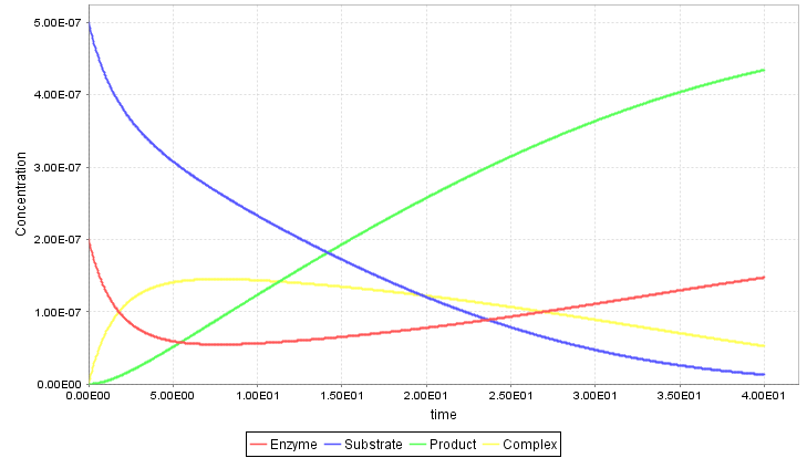
Figure 1: Numerical solution of the Michaelis-Menten ODE system (2); rate constants: $k_{f}=10^{6},k_{b}=10^{-4}$, and $k_{p}=0.1$; initial concentrations: $E={\bf 2\times 10^{-7}},S={\bf 5\times 10^{-7}},P=C=0$.

2.3 The Stochastic Simulation Algorithm

Consider a system made of $M$ chemical reactions $R_{1},\ldots,R_{M}$ and $N$ chemical species. The state of the system at time $t$ is given by the vector ${\bf x}(t)\in\mathbb{N}^{N}$, i.e., the state is just the number of molecules for each species. (Again, we drop time dependency and just write ${\bf x}$.) The state of the system changes only when a reaction fires. Reaction $R_{j}$ changes the state from ${\bf x}$ to ${\bf x}+{\bf v}_{j}$, where ${\bf v}_{j}\in\mathbb{Z}^{N}$ denotes the (fixed) state change caused by $R_{j}$. Therefore, we must have $M$ state change vectors ${\bf v}$’s, one for each reaction. Note that the elements of a vector ${\bf v}_{j}$ are negative integers when molecules of a particular species are consumed, while positive integers denote production of species.

The fundamental element in the Stochastic Simulation Algorithm (SSA) [14] is the propensity function. To each reaction $R_{j}$ there corresponds a function $a_{j}:\mathbb{N}^{N}\rightarrow\mathbb{R}^{\geqslant 0}$, which describes a probability law as follows:

$$\text{Prob}(R_{j}\;\text{fires in interval}\;[t,t+dt)\,|\,{\bf x})=a_{j}({\bf x})dt\ .$$

Note that the propensity functions do not explicitly depend on time (but remember that ${\bf x}$ is the state at time $t$).

It can be shown that the (infinitesimal) probability that the system evolves away from ${\bf x}$ in the time interval $[t+\tau,t+\tau+d\tau)$ is

$$\text{Prob}(\text{system evolves}\ \text{in}\;[t+\tau,t+\tau+d\tau)\,|\,{\bf x})=a_{0}({\bf x})e^{-a_{0}({\bf x})\tau}d\tau$$ (3)

where $a_{0}({\bf x})=\sum_{j=1}^{M}a_{j}({\bf x})$. Therefore, the time of the next reaction is a random variable distributed as an exponential with mean $\frac{1}{a_{0}({\bf x})}$. Now, the probability that system actually chooses reaction $R_{j}$ is

$$\text{Prob}(R_{j}\ \text{fires}\,|\,{\bf x})=\frac{a_{j}({\bf x})}{a_{0}({\bf x})}$$ (4)

thus a discrete random variable. Therefore, by (conditional) event independence we multiply (3) and (4) to get

$$\text{Prob}(R_{j}\ \text{fires in}\;[t+\tau,t+\tau+d\tau)\,|\,{\bf x})=a_{0}({\bf x})e^{-a_{0}({\bf x})\tau}d\tau\cdot\frac{a_{j}({\bf x})}{a_{0}({\bf x})}\ .$$ (5)

The SSA thus simulates the evolution of the system by sampling two random variables: it samples the time of the next reaction according to the density (3), and it selects which reaction to fire by sampling from the distribution (4). The simulation stops when a given time bound $T$ is reached (see Algorithm 1).

// initialise time and system state

$\tau$ := 0;

${\bf x}:={\bf x}_{0}$;

// simulate up to time $T$

while $\tau\leqslant T$ do

       evaluate $a_{j}({\bf x})$ ($1\leqslant j\leqslant M$) and $a_{0}({\bf x})$;

       $t:=\text{sample time step from density of Eq.}$ (3);

       $j:=\text{sample reaction index from distribution of Eq.}$ (4);

       $\tau:=\tau+t$;

       ${\bf x}:={\bf x}+{\bf v}_{j}$;

      

end

Algorithm 1 The Stochastic Simulation Algorithm

From (3) and (4) we see that the propensity functions actually define a time-homogeneous Continuous-Time Markov Chain (CTMC), whose state space can possibly be (countably) infinite. For finite-state CTMCs, it can be shown that during a finite simulation (i.e., $T<\infty$) the state space explored is finite with probability one. That is, the state transition sequences of finite CTMCs satisfy the non-zenoness property [1]. In our setting, this means that the SSA will fire an infinite number of reactions in finite time with probability zero.

To complete the description of the SSA, we only need to define explicitly the propensity functions. As for ODE modelling, one may generally assume mass-action kinetics. For example, the stochastic rate law (or propensity) for a unimolecular reaction such as the Michaelis-Menten production reaction is $c_{p}{\bf[se]}$, where $c_{p}$ is the stochastic rate constant for the reaction and ${\bf[se]}$ is the quantity of species $SE$ (remember that ${\bf[se]}$ is a natural number.) For bimolecular reactions such as the forward reaction, the rate law is $c_{f}{\bf[s][e]}$, where ${\bf[s]}$ and ${\bf[e]}$ are the quantity of species $S$ and $E$, respectively. For the case of a general reaction, and to see how the stochastic rate constants can be obtained from the deterministic (ODE) constants, the interested reader can find more details in [36], for example.

In Figure 2 we plot an exemplary run of the SSA on the Michaelis-Menten set of reactions (1). The initial molecule numbers and stochastic rate constants were converted from the respective deterministic (ODE) values used for generating Figure 1. As we can see from the plot in Figure 2, the temporal evolution of the species’ quantity fluctuates, and it is not a smooth line as in the ODE solution of Figure 1. Typically, no two SSA runs are the same, except in the case of large initial molecule numbers — see Section 2.5 below.

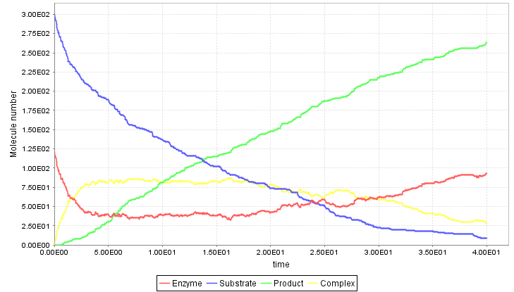
Figure 2: An exemplary run of the SSA on the Michaelis-Menten reaction system (1); stochastic rate constants: $c_{f}=1.66\times 10^{-3},c_{b}=10^{-4}$, and $c_{p}=0.1$; initial molecule numbers: $E={\bf 121},S={\bf 300},P=C=0$.

In Figure 3 we give an example of what happens instead at low molecule numbers: stochastic effects are even more preponderant than in the setting of Figure 2, and the temporal evolution of the species seems to be very “noisy”. Also, note that the CTMC nature of the model is more evident here. In fact, it is easy to see time intervals (e.g., at about 17s) in which the species’ numbers do not change at all, meaning that no reaction has fired in those intervals.

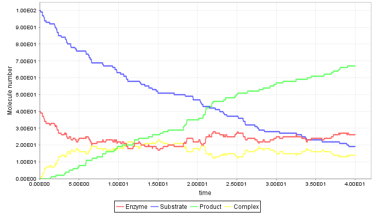
Figure 3: An exemplary run of the SSA on the Michaelis-Menten reaction system (1); stochastic rate constants: $c_{f}=1.66\times 10^{-3},c_{b}=10^{-4}$, and $c_{p}=0.1$; initial molecule numbers: $E={\bf 40},S={\bf 100},P=C=0$.

2.4 Probability Estimation

The SSA can be used in a simple Monte Carlo approach to estimate the probability of events such as

$$\xi=\text{within $T$ time units the state {\bf x}\ of the system will reach region O}$$

where $O\subset\mathbb{N}^{N}$. As usual, one can define a Bernoulli random variable whose success probability is Prob($\xi$). Then, the system is repeatedly simulated up to time $T$, while checking at every step whether ${\bf x}\in O$ (and stopping the simulation if that is true). Finally, to get an estimate of Prob$(\xi)$, we divide the number of “successful” trajectories - those where $\xi$ occurs - by the total number of trajectories (see Algorithm 2). One can use statistical estimation techniques (e.g., Chernoff bound) to get confidence intervals for the estimate, or use appropriate hypothesis tests.

In the SMC setting, the events $\xi$ are represented by formulae of a suitable temporal logic. In particular, formulae need to be decidable on a finite simulation trace, since any simulation must terminate at some point. An example of such formulae is

$${\bf F}^{25}(\text{\em Product}>40)$$

which is true if and only if within the next 25s the amount of Product will raise above 40. Essentially, SMC boils down to either estimating or hypothesis testing the probability of such properties.

$s:=0$;

for $i\leftarrow 1$ to $K$ do

       // initialise time and system state

       $\tau$ := 0;

       ${\bf x}:={\bf x}_{0}$;

       // simulate up to time $T$

       while $\tau\leqslant T$ do

             if ${\bf x}\in O$ then

                  // record occurrence of event $\xi$ and stop simulation

                   $s:=s+1$;

                   break

            end evaluate $a_{j}({\bf x})$ ($1\leqslant j\leqslant M$) and $a_{0}({\bf x})$;

             $t:=\text{sample time step from density of Eq.}$ (3);

             $j:=\text{sample reaction index from distribution of Eq.}$ (4);

             $\tau:=\tau+t$;

             ${\bf x}:={\bf x}+{\bf v}_{j}$;

            

      end

end return $\frac{s}{K}$

Algorithm 2 Probability estimation using the SSA

2.5 Relation with Differential Equation Models

It can be shown that, for any given finite volume, for high molecule numbers (hence high concentrations) the stochastic (CTMC) model can be very well approximated by its corresponding ODE model. On the other hand, for low molecule numbers the stochastic and ODE model will in general behave very differently. The same effects can be had if we fix the molecule numbers and vary the volume, of course. In Figure 4 we plot a run of the SSA on the Michaelis-Menten reactions (1) with a 100-fold increase of the initial molecule numbers with respect to those used in Figure 2. Notice how the species’ numbers evolve almost “continuously”, in a very similar way to the solutions of the corresponding ODE system plotted in Figure 5.

Figure 4: An exemplary run of the SSA on the Michaelis-Menten reaction system (1); stochastic rate constants: $c_{f}=1.66\times 10^{-3},c_{b}=10^{-4}$, and $c_{p}=0.1$; initial molecule numbers: $E={\bf 12,100},S={\bf 30,000},P=C=0$.

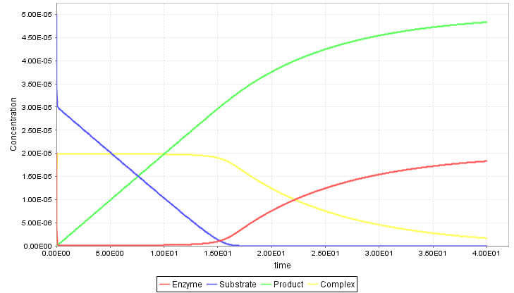
Figure 5: Numerical solution of the Michaelis-Menten ODE system (2); rate constants: $k_{f}=10^{6},k_{b}=10^{-4}$, and $k_{p}=0.1$; initial concentrations: $E={\bf 2\times 10^{-5}},S={\bf 5\times 10^{-5}},P=C=0$.

From a computational point of view, the cost of simulating a set of ODEs does not depend much on the initial conditions. However, it is easy to see that for high molecule numbers, the cost of simulating the CTMC reaction model increases significantly. In particular, the mean time of the next reaction is inversely proportional to the total number of molecules present in the system and the reaction rates — see Eq. (3). Therefore, to simulate a given amount of system time, the SSA will generate a much higher number of reaction events. This is the reason why many researchers are still actively investigating ways to speed up the SSA while maintaining a reasonable accuracy. The $\tau$-leaping technique is such an example [16, 30].

The ODE approximation of CTMCs in the context of biochemical modelling was formally proved in a 1992 paper by Gillespie [15], although in fact the general theory had been developed in 1970 by Kurtz [26]. The same theory has been recently introduced in performance modelling (but known as fluid flow approximation.)

3 Verification of Biological Models

3.1 Biochemical Reaction Networks

The idea of using a statistical (or Monte Carlo) approach for model checking stochastic biological models was introduced as early as 2006 by Calzone et al. [8]. In that paper, the authors outline a Monte Carlo approach for estimating the probability of (a finite variant of) LTL formulae over CTMC models of biochemical reactions, along the lines presented in Section 2.4. The authors do not discuss the type of statistical tests to be used, although they seem to hint at the Chernoff bound.

In a 2008 work, Clarke et al. [9] have applied Wald’s Sequential Probability Ratio Test (SPRT) [35] for verifying stochastic models of signalling pathways. Properties are expressed using a novel formalism, the Bounded Linear Temporal Logic (BLTL). This logic is essentially a variant of LTL in which temporal operators are equipped with a time bound. Also, BLTL can be seen as a sublogic of Metric Temporal Logic [25]. Previous approaches used a version of LTL defined over finite traces, with the addition of a time proposition representing the ‘global’ time of the simulation. Hence, BLTL offers better flexibility as every temporal operator has its own ‘clock’. We note that the use of the SPRT for statistical model checking was first introduced by Younes and Simmons’ in their pioneering paper [38].

A Bayesian approach to SMC was first introduced by Jha et al. in a 2009 paper [18]. In particular, the authors introduce a sequential version of the Bayes factor (hypothesis) test. It is a test for composite hypotheses, i.e., $p\leqslant\theta$ vs. $p>\theta$, where in our SMC setting $p$ is the unknown probability that a given property holds. Basically, the test starts with a prior distribution over $p$, which is then sequentially updated via Bayes’ theorem to a posterior distribution computed as a function of the prior and the likelihood of the simulated sample. On the other hand, we recall that the SPRT is in fact a test for simple hypotheses, i.e., $p=\theta_{1}$ vs. $p=\theta_{2}$ (where $0\leqslant\theta_{1}<\theta_{2}\leqslant 1$) and the so-called indifference region is the distance $\theta_{2}-\theta_{1}$. It can be shown that for a large class of distributions (including the SMC relevant Binomial) the SPRT can be used to decide the composite test $p\leqslant\theta_{1}$ vs. $p\geqslant\theta_{2}$, while respecting the same Type I and II error probabilities of the simple hypothesis test. The number of samples required by the SPRT is inversely proportional to the square of the size of the indifference region, while for the Bayes factor test a similar relation holds with respect to the distance between the threshold $\theta$ and the true probability of the given formula. Also, it can be shown that the SPRT is in fact the Bayes factor test for simple hypotheses with equal a priori probabilities.

In a 2012 paper, Ballarini et al. [3] have proposed a SMC approach in which properties are expressed in Hybrid Automata Stochastic Logic (HASL) instead of one of the usual variants of temporal logic. Basically, a HASL property is made of a linear hybrid automaton and an arithmetic expression over the so-called data variables of the automaton. The goal of the SMC procedure is to estimate the value of the expression by simulating the (synchronous) composition of the model and the HASL automaton. The whole approach has been implemented in the COSMOS tool [2]. The authors demonstrate their technique by analysing stochastic models of gene networks with delayed dynamics. The introduction of a time delay is meant to capture more faithfully the actual timings involved in fundamental gene expression processes, i.e., transcription and translation. A drawback of this approach is the difficulty of writing HASL specifications that capture a given behaviour,e.g., oscillations. That essentially amounts to specify an automaton, and hence it might constitute a roadblock for non-expert users.

Koh et al.[24] have presented OSM, a new hypothesis test algorithm based on the SPRT, in which one does not have to specify the indifference region. Also, if this new algorithm cannot reach a conclusion within an allotted amount of time, the p-value of the two hypotheses (with respect to the samples seen so far) will be computed and returned to the user, who is then left with the final choice. The approach is a simple modification of Younes’ SPRT version with error control in the indifference region [37]. The key modification is a dynamic adjustment of the indifference region, from the largest possible value (i.e., 1) to the largest value that enable a SPRT decision between the null and the alternative hypothesis. The approach is applied for verifying temporal logic properties of a neuron subnet model of the worm C. elegans. The authors have empirically shown that their algorithm is more efficient than Younes’ original algorithm.

In Table 1 we summarise the various hypothesis tests mentioned in this Section.

Test	Problem addressed	Notes
SPRT [35]	$H_{0}:p=\theta_{1}$ vs. $H_{1}:p=\theta_{2}$	Also usable for
	where $0\leqslant\theta_{1}<\theta_{2}\leqslant 1$	$H_{0}:p\leqslant\theta_{1}$ vs. $H_{1}:p\geqslant\theta_{2}$
Bayes [18]	$H_{0}:p\leqslant\theta$ vs. $H_{1}:p>\theta$	Easy to modify for
	where $0<\theta<1$	$H_{0}:p\leqslant\theta_{1}$ vs. $H_{1}:p\geqslant\theta_{2}$
OSM [24]	$H_{0}:p\leqslant\theta$ vs. $H_{1}:p>\theta$	Based on the SPRT;
	where $0<\theta<1$	may return ‘undecided’

Table 1: Hypothesis testing techniques used in SMC; $p$ is the (unknown) mean of a Bernoulli distribution.

3.2 Other Biological Models

In a recent paper, Sankaranarayanan and Fainekos [32] have analysed the risks resulting from malfunctioning of insulin infusion pumps by modelling the insuline-glucose regulatory system. The model is essentially a Stateflow/Simulink hybrid system with nonlinear differential equations. Randomness is introduced by sampling several initial model parameters, such as meal time, pump calibration error, etc. The author have used Bayesian SMC [40] for estimating the probabilities of hyper- and hypoglycemia conditions, which are expressed as Metric Temporal Logic formulae. (In Section 4.1 we survey another work on the synthesis of safe controllers for insulin infusion pumps.)

Jha and Langmead [21] have investigated SMC in the context of rare-event behaviour in biological models expressed as stochastic differential equations (SDEs). The behaviours under study are expressed as BLTL formulae, while the systems studied are models of tumour progression. The verification problem is then to decide whether a given property is satisfied with a probability larger than a threshold — the problem thus reduces to hypothesis testing. The technique presented basically uses importance sampling to simulate a higher proportion of the ‘important’, i.e., rare, event from the SDE model. Then, a modified version of the Bayes factor test is used to decide the verification problem. The authors have also derived bounds on the probability of returning the wrong answer.

4 Parameter Estimation and Synthesis

The parameter estimation problem is to determine a combination of model parameters that fit experimental results (e.g., time-series data) or some well-specified behaviour (e.g., temporal logic formulae.) Parameter synthesis is similarly defined, except that one is instead interested in determining sets of parameters that satisfy the given constraints. Obviously, parameter synthesis is a much harder problem than parameter estimation. In the setting involving biochemical reactions, the parameters in question are the reaction rate constants of the model.

4.1 Parameter Estimation

In a 2006 paper, Calzone et al. [8] suggested that a SMC approach could be used to learn model parameters from LTL specifications. However, the authors also argued that such an approach would not be practical because of the complexity of the (stochastic) simulation and model checking. Hence, no result for stochastic models is actually reported in the paper, although the authors do apply their method to continuous deterministic models [8]. Also, note that the procedure could be used for parameter synthesis, since it is essentially a simple sweep of the whole (compact) parameter space, up to a certain numerical precision.

Donaldson and Gilbert [11] presented in 2008 a SMC approach for estimating reaction rate constants from temporal logic specifications and numerical constraints. In particular, the temporal logic used is a variant of LTL that allows for arithmetic expressions and general functions of the state (e.g., derivative) as atomic properties. The search in the parameter space is performed by a genetic algorithm whose objective is minimising the distance between the behaviour of the current model and the target model. The authors motivate the use of genetic algorithms because of their ability to avoid getting trapped in local optima. The authors apply the technique to a large model, and estimate the values of all its 65 parameters. Even though the model analysed is continuous, we have reported here this work because the authors defined their framework to be usable on stochastic models, too.

In a 2012 paper, Jha et al. [19] have studied the problem of synthesising control laws for insulin infusion pumps from safety specifications expressed in BLTL. The glucose-insulin model is a relatively simple ODE model, while the controller implements a Proportional Integral Derivative control law, described by an equation containing both integration and derivation (of course, the entire model can be converted to an equivalent ODE-only model.) The task is to find values for the three parts of the control law in such a way that the controller meets its safety specifications. This is achieved by an exhaustive sweep of the (bounded) parameter space. Also, the authors assume that some of the model’s parameters are random, so that the ODE model becomes suitable for SMC.

Recently, Palaniappan et al. [29] have introduced a SMC-based approach for calibrating ODE models of signalling pathways. In particular, the authors present a technique for parameter estimation with respect to behavioural specification and experimental data that are described as BLTL formulae. The idea is quite straightforward: the unknown parameters are sampled from (usually uniform) distributions, the resulting ODE model is then simulated, and finally the SPRT is used to decide whether the given probabilistic BLTL formula is satisfied or not. An evolutionary algorithm is used to guide the search in the parameter space, through a goodness-of-fit function that measures how well the current model agrees with the behavioural specification and the experimental data. The same function is also used to perform sensitivity analysis. The authors have successfully applied their approach to a reasonably large (105 ODEs, 39 unknown parameters) pathway model.

In the past year, verification and statistical model checking have started embracing the notion of robustness for temporal logic. The idea is to endow temporal logic with a suitable quantitative semantics that: 1) generalises the standard (Boolean) semantics; and 2) gives a measure of “how much” a temporal formula is true. For example, consider the formula ${\bf F}(x>0)$: intuitively, a trace would satisfy the formula more robustly if the maximum value of $x$ in such a trace is higher (conversely, if $x$ is always negative then the formula robustness will be negative, and the Boolean semantics is false, of course). Donzé et al. [12] defined a quantitative semantics for STL (a generalisation of LTL in which the Until operator may be equipped with an interval) and gave algorithms for computing the robustness of a STL formula with respect to time-series data (or traces).

Bartocci et al. [4] have extended the notion of STL robustness to stochastic (CTMC) models. In this setting, robustness becomes a random variable defined on the space of the stochastic model’s traces. Also, one obtains the robustness distribution, i.e., the probability distribution associated to the robustness random variable. For example, the mean of the robustness distribution gives the ‘average’ robustness of the model traces. The authors use the robustness distribution to guide parameter estimation for CTMC models, i.e., find a parameter combination such that the model satisfies a given STL formula with probability greater than a given threshold, while maximising its robustness. In particular, statistical model checking (on STL properties) is used for building a statistical emulator of the robustness distribution, upon which an optimisation algorithm is then used to identify the parameter combination. The use of a statistical emulator is motivated by the fact that evaluating the true robustness distribution is computationally onerous.

Česka et al. [34] explore another definition of robustness, based on an earlier notion by Kitano [23]. Basically, they define robustness as the expected value of an evaluation function with respect to a probability measure over a space of system perturbations. The evaluation function is defined over the perturbation space, and it determines to what degree the “wild-type” behaviour of the system is preserved by a given perturbation. The evaluation function is based on the probability that the model satisfies a given CSL formula. To compute the expectation, the authors employ a novel probabilistic model checking technique that can provide bounds on the evaluation function, since computing the function for every perturbation point is unfeasible. Even though the current approach is based on probabilistic model checking, the authors report that they are looking into extending it towards statistical model checking in order to cope with dimensionally large parameter spaces.

4.2 Parameter Synthesis

In [20], Jha and Langmead present three algorithms for synthesising kinetic constants of stochastic (CTMC) reaction models given a probabilistic temporal logic specification, a parameter search region (a multi-dimensional real compact set), and an error tolerance. The algorithms decide whether there are parameters in the region that satisfy the specification (up to the given error) or whether the model is unfeasible within the given parameter region. The difference between the three algorithms lies in the output: two algorithms return, if it exists, a subregion of the parameter search space for which every point is guaranteed to satisfy the probabilistic temporal formula — so called feasible region. (The second algorithm uses an abstraction-refinement technique to speed up convergence.) The third algorithm returns instead the point in the feasible region that maximises the probability that the temporal logic formula is true, thereby solving parameter estimation.

The algorithms rely on the fact that the probability density in the SSA is a continuous function of the kinetic parameters, and thus uniformly continuous as the parameter region is a compact set. Therefore, the probability that the formula is true can be bounded accordingly on any subset of the parameter region. This is the key result that enable the parameter synthesis algorithms: basically, one first partitions the parameter region according to the error tolerance selected by the user, and then one point is randomly sampled in each partition sets. If the point satisfies the formula then the entire partition set is added to the feasible region, otherwise that partition set is rejected. Note that the size of each partition set is computed in such a way that for any point in a given partition set the probability of the formula being true does not change more than the error tolerance. The third (parameter estimation) algorithm works in a similar way except that it uses the gradient of the satisfaction probability of the formula to guide the search in the parameter region. The authors successfully apply their parameter synthesis techniques to a six-dimensional biological model, while their parameter estimation algorithm was able to scale up to eleven parameters. Finally, we remark that all the results given by the algorithms are necessarily approximate, because of general undecidability results for complex first order formulae over the reals [31, 13].

5 Tool support

In this Section we give a brief overview of software tools that support SMC, which are now in growing numbers. We have the aforementioned COSMOS tool [2] for SMC of stochastic hybrid automata, which has been applied for studying gene networks. The ANIMO tool [33] allows the user to build signalling pathway models in a graphical way. The models can be simulated and also verified using the UPPAAL model checker [28], since the underlying semantics is given as timed automata.

PLASMA-Lab [5] is a very flexible library for embedding statistical model checking capabilities in general simulation tools. In particular, PLASMA-Lab can verify biological models expressed as CTMCs via its own modelling language and simulator; the property language is BLTL extended with several temporal operators for minimum, maximum and mean of a variable. PLASMA-Lab can also efficiently handle the verification of rare events, i.e., properties that are satisfied with extremely low probability.

PRISM [27] is a very powerful model checker that can handle a large variety of stochastic models (discrete-time MC, CTMC, Markov Decision Processes, Probabilistic Automata, etc.) and temporal logics (CSL, LTL, etc.). For our application area, PRISM’s modelling language can directly support CTMCs, and temporal logic verification can be performed either numerically or via SMC. The former is very precise, but it can become quickly infeasible for large models. PRISM has been used for many case studies in systems biology.

UPPAAL-SMC [7] extends UPPAAL by adding SMC capabilities for networks of stochastic hybrid automata. The modelling language is quite rich, allowing the user to define hybrid models containing both CTMCs and ODEs. UPPAAL-SMC has been used for studying a number of biological case studies, e.g., a genetic oscillator [10]. Also, UPPAAL-SMC supports SBML models (see below) through an internal conversion utility.

Finally, the Systems Biology Markup Language (SBML) [17] is a very much used language for interchanging computational biology models. It is supported by most tools for scientific computation such as, e.g., MATLAB (via the SimBiology package or SBMLToolbox [22]). A list of SBML compliant tools is available on http://sbml.org.

6 Conclusions

Statistical model checking (SMC) is becoming increasingly useful for analysing stochastic biological models, as witnessed by a number of recent works surveyed in this paper. The use of SMC for ‘traditional’ verification of biological models appeared first, and it is perhaps now the only way to tackle the usually large and complex models arising from biological applications. Now, SMC is being investigated for other difficult problems, such as parameter estimation and parameter synthesis, which are even more central to systems biology. It is expected that computer science researchers will make use of the rich literature on parameter estimation and synthesis from other disciplines, e.g., control theory. The estimation of rare-event probabilities for biological models might represent another area for further work. It is well known that standard SMC would require extremely large sample sizes to estimate accurately very low probabilities. Finally, a whole new area of possible application for SMC techniques is represented by sequence analysis. In that field, hidden Markov models are routinely used to analyse DNA sequences, and one could conceivably use some variant of temporal logic to express sequence properties and then apply SMC for verification.

References

- [1] C. Baier, B. R. Haverkort, H. Hermanns, and J.-P. Katoen. Model-checking algorithms for continuous-time Markov chains. IEEE Trans. Software Eng., 29(6):524–541, 2003.
- [2] P. Ballarini, H. Djafri, M. Duflot, S. Haddad, and N. Pekergin. COSMOS: A statistical model checker for the hybrid automata stochastic logic. In QEST, pages 143–144, 2011.
- [3] P. Ballarini, J. Mäkelä, and A. S. Ribeiro. Expressive statistical model checking of genetic networks with delayed stochastic dynamics. In CMSB, volume 7605 of LNCS, pages 29–48, 2012.
- [4] E. Bartocci, L. Bortolussi, L. Nenzi, and G. Sanguinetti. On the robustness of temporal properties for stochastic models. In HSB, volume 125 of EPTCS, pages 3–19, 2013.
- [5] B. Boyer, K. Corre, A. Legay, and S. Sedwards. PLASMA-lab: A flexible, distributable statistical model checking library. In QEST, volume 8054 of LNCS, pages 160–164, 2013.
- [6] L. Brim, M. Česka, and D. Šafránek. Model checking of biological systems. In SFM, volume 7938 of LNCS, pages 63–112, 2013.
- [7] P. E. Bulychev, A. David, K. G. Larsen, M. Mikucionis, D. B. Poulsen, A. Legay, and Z. Wang. UPPAAL-SMC: Statistical model checking for priced timed automata. In QAPL, volume 85 of EPTCS, pages 1–16, 2012.
- [8] L. Calzone, N. Chabrier-Rivier, F. Fages, and S. Soliman. Machine learning biochemical networks from temporal logic properties. In T. Comp. Sys. Biology, volume 4220 of LNCS, pages 68–94, 2006.
- [9] E. M. Clarke, J. R. Faeder, C. J. Langmead, L. A. Harris, S. K. Jha, and A. Legay. Statistical model checking in BioLab: Applications to the automated analysis of T-cell receptor signaling pathway. In CMSB, volume 5307 of LNCS, pages 231–250, 2008.
- [10] A. David, K. G. Larsen, A. Legay, M. Mikucionis, D. B. Poulsen, and S. Sedwards. Runtime verification of biological systems. In ISoLA (1), volume 7609 of LNCS, pages 388–404, 2012.
- [11] R. Donaldson and D. Gilbert. A model checking approach to the parameter estimation of biochemical pathways. In CMSB, volume 5307 of LNCS, pages 269–287, 2008.
- [12] A. Donzé, T. Ferrère, and O. Maler. Efficient robust monitoring for STL. In CAV, volume 8044 of LNCS, pages 264–279, 2013.
- [13] S. Gao, J. Avigad, and E. M. Clarke. Delta-decidability over the reals. In LICS, pages 305–314, 2012.
- [14] D. T. Gillespie. A general method for numerically simulating the stochastic time evolution of coupled chemical reactions. J. Comp. Phys., 22:403–434, 1976.
- [15] D. T. Gillespie. A rigorous derivation of the chemical master equation. Physica A, 188:404–425, 1992.
- [16] D. T. Gillespie. Approximate accelerated stochastic simulation of chemically reacting systems. J. Chem. Phys., 115(4):1716–1733, 2001.
- [17] M. Hucka et al. The systems biology markup language (SBML): a medium for representation and exchange of biochemical network models. Bioinformatics, 19(4):524–531, 2003.
- [18] S. K. Jha, E. M. Clarke, C. J. Langmead, A. Legay, A. Platzer, and P. Zuliani. A Bayesian approach to model checking biological systems. In CMSB, volume 5688 of LNCS, pages 218–234, 2009.
- [19] S. K. Jha, R. G. Dutta, C. J. Langmead, S. Jha, and E. Sassano. Synthesis of insulin pump controllers from safety specifications using Bayesian model validation. IJBRA, 8(3/4):263–285, 2012.
- [20] S. K. Jha and C. J. Langmead. Synthesis and infeasibility analysis for stochastic models of biochemical systems using statistical model checking and abstraction refinement. Theor. Comput. Sci., 412(21):2162–2187, 2011.
- [21] S. K. Jha and C. J. Langmead. Exploring behaviors of stochastic differential equation models of biological systems using change of measures. BMC Bioinformatics, 13(S-5):S8, 2012.
- [22] S. M. Keating, B. J. Bornstein, A. Finney, and M. Hucka. SBMLToolbox: an SBML toolbox for MATLAB users. Bioinformatics, 22(10):1275–1277, 2006.
- [23] H. Kitano. Biological robustness. Nature Review Genetics, 5(11):826–837, 2004.
- [24] C. H. Koh, S. K. Palaniappan, P. S. Thiagarajan, and L. Wong. Improved statistical model checking methods for pathway analysis. BMC Bioinformatics, 13(S-17):S15, 2012.
- [25] R. Koymans. Specifying real-time properties with metric temporal logic. Real-time Systems, 2(4):255–299, 1990.
- [26] T. G. Kurtz. Solutions of ordinary differential equations as limits of pure jump Markov processes. J. Appl. Prob., 7(1):49–58, 1970.
- [27] M. Kwiatkowska, G. Norman, and D. Parker. PRISM 4.0: Verification of probabilistic real-time systems. In CAV, volume 6806 of LNCS, pages 585–591, 2011.
- [28] K. G. Larsen, P. Pettersson, and W. Yi. UPPAAL in a nutshell. STTT, 1(1-2):134–152, 1997.
- [29] S. K. Palaniappan, B. M. Gyori, B. Liu, D. Hsu, and P. S. Thiagarajan. Statistical model checking based calibration and analysis of bio-pathway models. In CMSB, volume 8130 of LNCS, pages 120–134, 2013.
- [30] M. Rathinam, L. R. Petzold, Y. Cao, and D. T. Gillespie. Stiffness in stochastic chemically reacting systems: The implicit tau-leaping method. J. Chem. Phys., 119(24):12784–12794, 2003.
- [31] D. Richardson. Some undecidable problems involving elementary functions of a real variable. The Journal of Symbolic Logic, 33(4):pp. 514–520, 1968.
- [32] S. Sankaranarayanan and G. E. Fainekos. Simulating insulin infusion pump risks by in-silico modeling of the insulin-glucose regulatory system. In CMSB, volume 7605 of LNCS, pages 322–341, 2012.
- [33] S. Schivo, J. Scholma, B. Wanders, R. A. U. Camacho, P. E. van der Vet, M. Karperien, R. Langerak, J. van de Pol, and J. N. Post. Modelling biological pathway dynamics with timed automata. In BIBE, pages 447–453. IEEE, 2012.
- [34] M. Česka, D. Šafránek, S. Dražan, and L. Brim. Robustness analysis of stochastic biochemical systems. PLoS ONE, 9(4), 2014.
- [35] A. Wald. Sequential test of stastistical hypotheses. Annals of Math. Stat., 16(2):117–186, 1945.
- [36] D. J. Wilkinson. Stochastic Modelling for Systems Biology. CRC Press, 2nd edition, 2011.
- [37] H. L. S. Younes. Error control for probabilistic model checking. In VMCAI, volume 3855 of LNCS, pages 142–156, 2006.
- [38] H. L. S. Younes and R. G. Simmons. Probabilistic verification of discrete event systems using acceptance sampling. In CAV, volume 2404 of LNCS, pages 223–235, 2002.
- [39] F. Zhang, M. Yeddanapudi, and P. Mosterman. Zero-crossing location and detection algorithms for hybrid system simulation. IFAC World Congress, pages 7967–7972, 2008.
- [40] P. Zuliani, A. Platzer, and E. M. Clarke. Bayesian statistical model checking with application to Simulink/Stateflow verification. In HSCC, pages 243–252, 2010.