Abstract

The off-diagonal Bethe ansatz method is generalized to the high spin integrable systems associated with the $su(2)$ algebra by employing the spin-$s$ isotropic Heisenberg chain model with generic integrable boundaries as an example. With the fusion techniques, certain closed operator identities for constructing the functional $T-Q$ relations and the Bethe ansatz equations are derived. It is found that a variety of inhomogeneous $T-Q$ relations obeying the operator product identities can be constructed. Numerical results for two-site $s=1$ case indicate that an arbitrary choice of the derived $T-Q$ relations is enough to give the complete spectrum of the transfer matrix.

PACS: 75.10.Pq, 02.30.Ik, 05.30.Jp

Keywords: Spin chain; Reflection equation; Bethe Ansatz; $T-Q$ relation

1 Introduction

Among integrable quantum spin chains, the $su(2)$-invariant spin-$s$ Heisenberg chain is particularly interesting due to its relationship to the Wess-Zumino-Novikov-Witten (WZNW) models [1, 2, 3, 4] and lower dimensional super-symmetric quantum field theories [5] such as the super-symmetric sine-Gordon model [6], the fractional statistics [7] and the multi-channel Kondo problem [8, 9, 10] when it couples to an impurity spin. The $s=1$ integrable spin chain model was firstly proposed by Zamalodchikov and Fateev [11]. Its generalization to arbitrary $s$ cases was subsequently constructed via the fusion techniques [12] based on the fundamental $s=\frac{1}{2}$ representations of the Yang-Baxter equation [13, 14]. Those observations allow one to diagonalize the models with periodic boundary conditions in the framework of algebraic Bethe ansatz method (for example, see [15]). On the other hand, the discovery of the boundary Yang-Baxter equation or the reflection equation [16, 17] directly stimulated the studies on the exact solutions of the quantum integrable models with boundary fields. A striking feature of the reflection equation is that it allows non-diagonal solutions [18, 19], which leads to the corresponding eigenvalue problem quite frustrated. Many efforts had been made [20, 21, 22, 23, 24, 25, 26, 27, 28, 29, 30, 31, 32] to approach this nontrivial problem. However, in a long period of time, the Bethe ansatz solutions could only be obtained for either constrained boundary parameters [20] or special crossing parameters [21] associated with spin-$\frac{1}{2}$ chains or with spin-$s$ chains [33, 34, 35, 36].

Recently, based on the fundamental properties of the $R$-matrix and the $K$-matrices for quantum integrable models, a systematic method for solving the eigenvalue problem of integrable models with generic boundary conditions, i.e., the off-diagonal Bethe ansatz (ODBA) method was proposed in [37] and several long-standing models [37, 38, 39] were then solved. Subsequently, the nested-version of ODBA for the models associated with $su(n)$ algebra [40], the application to the integrable models beyond $A$-type [41] and the thermodynamic analysis based on the ODBA solutions [42] were developed. We remark that two other promising methods, namely, the $q$-Onsager algebra method [43] and the separation of variables (SoV) method [31, 44] were also used to approach the spin-$\frac{1}{2}$ chains with generic integrable boundaries. Especially, the eigenstate problem for such kind of models with generic inhomogeneity was first approached via the SoV method [31]. A set of Bethe states for was then constructed in [45] and a method for retrieving the Bethe states based on the inhomogeneous $T-Q$ relation [37] and the SoV basis [31] was developed in [46]. The latter method allows one to reach the homogeneous limit of the SoV eigenstates and provides a clear connection among the SoV approach, the algebraic Bethe Ansatz and the ODBA.

The high spin models with periodic [11, 12, 15] and diagonal [47, 48, 49] boundaries have been extensively studied. Even the most general integrable boundary condition (corresponding to the non-diagonal reflection matrix) for the spin-$1$ model has been known for many years [50], the exact solutions of the models with non-diagonal boundaries were known only for some special cases such as the boundary parameters obeying some constraint [33] or the crossing parameter taking some special value (e.g., roots of unity) [34, 35]. In this paper, we show that the ODBA method can also be applied to the $su(2)$-invariant spin-$s$ chain with generic crossing parameter and generic integrable boundaries . The outline of the paper is the following: Section 2 serves as an introduction to some notations and the fusion procedure. In Section 3, after briefly reviewing the fusion hierarchy [33] of the high spin transfer matrices we derive certain closed operator product identities for the fundamental spin-$(\frac{1}{2},s)$ transfer matrix by using some intrinsic properties of the high spin $R$-matrix ($R^{(s,s)}(u)$) and $K$-matrices ($K^{\pm(s)}(u)$). The asymptotic behavior of the transfer matrix is also obtained. Section 4 is devoted to the construction of the inhomogeneous $T-Q$ relations and the corresponding Bethe ansatz equations (BAEs). Taking the spin-$1$ XXX chain as an example, we present numerical results for the model with some small number of sites, which indicate that an arbitrary choice of the derived $T-Q$ relations is enough to give the complete set of spectrum of the transfer matrix. In section 5, we summarize our results and give some discussions. In Appendix A, we prove that each solution of our functional equations can be parameterized in terms of a variety of inhomogeneous $T-Q$ relations and therefore that different $T-Q$ relations only indicate different parameterizations but not new solutions.

2 Transfer matrices for the spin-$s$ XXX spin chain

2.1 Fusion of the $R$-matrices and the $K$-matrices

Throughout, $V_{i}$ denotes a $(2l_{i}+1)$-dimensional linear space ($\mathbb{C}^{2l_{i}+1}$) which endows an irreducible representation of $su(2)$ algebra with spin $l_{i}$. The $R$-matrix $R^{(l_{i},l_{j})}_{ij}(u)$, denoted as the spin-$(l_{i},l_{j})$ $R$-matrix, is a linear operator acting in $V_{i}\otimes V_{j}$. The $R$-matrix satisfies the following quantum Yang-Baxter equation (QYBE) [13, 14]

$$R_{12}^{(l_{1},l_{2})}(u-v)R_{13}^{(l_{1},l_{3})}(u)R_{23}^{(l_{2},l_{3})}(v)=R_{23}^{(l_{2},l_{3})}(v)R_{13}^{(l_{1},l_{3})}(u)R_{12}^{(l_{1},l_{2})}(u-v).$$ (2.1)

Here and below we adopt the standard notations: for any matrix $A\in{\rm End}({V})$, $A_{j}$ is an embedding operator in the tensor space ${V}\otimes{V}\otimes\cdots$, which acts as $A$ on the $j$-th space and as identity on the other factor spaces; $R_{ij}(u)$ is an embedding operator of $R$-matrix in the tensor space, which acts as identity on the factor spaces except for the $i$-th and $j$-th ones.

The fundamental spin-$(\frac{1}{2},s)$ $R$-matrix $R^{(\frac{1}{2},s)}_{12}(u)$ defined in spin-$\frac{1}{2}$ (i.e., two-dimensional) auxiliary space and spin-$s$ (i.e., $(2s+1)$-dimensional) quantum space is given by [12]

$$R^{(\frac{1}{2},s)}_{12}(u)=u+\frac{\eta}{2}+\eta\,\vec{\sigma}_{1}\cdot\vec{S}_{2},$$ (2.2)

where $\eta$ is the crossing parameter, $\vec{\sigma}$ are the Pauli matrices and $\vec{S}$ are the spin-$s$ realization of the $su(2)$ generators. For the simplest case, i.e., $s=\frac{1}{2}$ case the corresponding $R$-matrix reads

$$R^{(\frac{1}{2},\frac{1}{2})}(u)=\left(\begin{array}[]{cccc}u+\eta&0&0&0\\ 0&u&\eta&0\\ 0&\eta&u&0\\ 0&0&0&u+\eta\end{array}\right).$$ (2.7)

Besides the QYBE (2.1), the $R$-matrix (2.7) also enjoys the following properties,

$$\mbox{Initial condition}:\,R^{(\frac{1}{2},\frac{1}{2})}_{12}(0)=\eta P_{12},$$ (2.8)

$$\mbox{Unitary relation}:\,R^{(\frac{1}{2},\frac{1}{2})}_{12}(u)R^{(\frac{1}{2},\frac{1}{2})}_{21}(-u)=-\xi(u)\,{\rm id},\quad\xi(u)=(u+\eta)(u-\eta),$$ (2.9)

$$\mbox{Crossing relation}:\,R^{(\frac{1}{2},\frac{1}{2})}_{12}(u)=V_{1}\{R^{(\frac{1}{2},\frac{1}{2})}_{12}\}^{t_{2}}(-u-\eta)V_{1},\quad V=-i\sigma^{y},$$ (2.10)

$$\mbox{PT-symmetry}:\,R^{(\frac{1}{2},\frac{1}{2})}_{12}(u)=R^{(\frac{1}{2},\frac{1}{2})}_{21}(u)=\{R^{(\frac{1}{2},\frac{1}{2})}\}^{t_{1}\,t_{2}}_{12}(u),$$ (2.11)

$$\mbox{Fusion conditions}:\,R^{(\frac{1}{2},\frac{1}{2})}_{12}(\pm\eta)=\eta(\pm 1+P_{12})=\pm 2\eta P_{12}^{\pm}.$$ (2.12)

Here $R^{(\frac{1}{2},\frac{1}{2})}_{21}(u)=P_{12}R^{(\frac{1}{2},\frac{1}{2})}_{12}(u)P_{12}$ with $P_{12}$ being the permutation operator and $t_{i}$ denotes transposition in the $i$-th space. Using the fusion procedure [12] the spin-$(\frac{1}{2},s)$ $R$-matrix $R^{(\frac{1}{2},s)}_{12}(u)$ can be obtained by the symmetric fusion of the spin-$(\frac{1}{2},\frac{1}{2})$ $R$-matrix

$$R^{({1\over 2},s)}_{a\{1\cdots 2s\}}(u)=\frac{1}{\prod_{k=1}^{2s-1}(u+(\frac{1}{2}-s+k)\eta)}P^{+}_{\{1\cdots 2s\}}\prod_{k=1}^{2s}\left\{R^{(\frac{1}{2},\frac{1}{2})}_{a,k}(u+(k-\frac{1}{2}-s)\eta)\right\}P^{+}_{\{1\cdots 2s\}},$$ (2.13)

where $P^{+}_{\{1\cdots 2s\}}$ is the symmetric projector given by

$$P^{+}_{1,\cdots,2s}=\frac{1}{(2s)!}\prod_{k=1}^{2s}\left(\sum_{l=1}^{k}P_{l\,k}\right).$$ (2.14)

Similarly, from the spin-$({1\over 2},s)$ $R$-matrix we can also extend the auxiliary space from $\frac{1}{2}$ to $j$ to obtain the spin-$(j,s)$ $R$-matrix by the symmetric fusion

$$R^{(j,s)}_{\{1\cdots 2j\}\{1\cdots 2s\}}(u)=P^{+}_{\{1\cdots 2j\}}\prod_{k=1}^{2j}\left\{R^{(\frac{1}{2},s)}_{k,\{1\cdots 2s\}}(u+(k-j-\frac{1}{2})\eta)\right\}P^{+}_{\{1\cdots 2j\}}.$$ (2.15)

We remark that the $R$-matrices in the products (2.15) and (2.13) are in the order of increasing $k$. One can demonstrate that the fused $R$-matrices (2.2) and (2.13) also satisfy the associated QYBE (2.1) with the help of (2.12). Direct calculation shows that the spin-$(s,s)$ $R$-matrix can be given by [12]

$$R^{(s,s)}=\prod_{j=1}^{2s}(u-j\eta)\,\sum_{l=0}^{2s}\prod_{k=1}^{l}\frac{u+k\eta}{u-k\eta}\,\mathbf{P}^{(l)},$$ (2.16)

where $\mathbf{P}^{(l)}$ is a projector acting on the tensor product of two spin-$s$ spaces and projects the tensor space into the irreducible subspace of spin-$l$ (i.e., $(2l+1)$-dimensional subspace). In particular, the fundamental spin-$(\frac{1}{2},s)$ and the fused spin-$(s,s)$ $R$-matrix possess the following important properties

$$\mbox{Unitary relation}:\,R^{(\frac{1}{2},s)}_{12}(u)R^{(s,\frac{1}{2})}_{21}(-u)=-(u+(\frac{1}{2}+s)\eta)(u-(\frac{1}{2}+s)\eta)\,{\rm id},$$ (2.17)

$$\mbox{ Initial condition}:\,R^{(s,s)}_{12}(0)=\eta^{2s}(2s)!P_{12},$$ (2.18)

$$\mbox{ Fusion condition}:\,R^{(s,s)}_{12}(-\eta)=(-1)^{2s}\eta^{2s}(2s+1)!\,\mathbf{P}^{(0)}.$$ (2.19)

The projector $\mathbf{P}^{(0)}$ projects the tensor product of two spin-$s$ spaces to the singlet space, namely,

$$\mathbf{P}^{(0)}=|\Phi_{0}\rangle\langle\Phi_{0}|,\quad|\Phi_{0}\rangle=\frac{1}{\sqrt{2s+1}}\sum_{l=0}^{2s}(-1)^{l}|s-l\rangle\otimes|-s+l\rangle,$$ (2.20)

where $\{|m\rangle,\,m=s,s-1,\ldots,-s\}$ spans the spin-$s$ representation of $su(2)$ algebra and forms an orthonormal basis of it. The very properties (2.17), (2.18) and (2.19) are the analogues of (2.9), (2.8) and (2.12) for the high spin case.

Having defined the fused-$R$ matrices, one can analogously construct the fused-$K$ matrices by using the methods developed in [47, 52] as follows. The fused $K^{-}$ matrices (e.g the spin-$j$ $K^{-}$ matrix) is given by

$$K^{-(j)}_{\{a\}}(u) = P_{\{a\}}^{+}\prod_{k=1}^{2j}\Bigg{\{}\left[\prod_{l=1}^{k-1}R^{(\frac{1}{2},\frac{1}{2})}_{a_{l}a_{k}}(2u+(k+l-2j-1)\eta)\right]$$ (2.21)

$$\times K^{-(\frac{1}{2})}_{a_{k}}(u+(k-j-\frac{1}{2})\eta)\Bigg{\}}P_{\{a\}}^{+}.$$

In this paper we adopt the most general non-diagonal spin-$\frac{1}{2}$ $K$-matrix $K^{-(\frac{1}{2})}(u)$ [18, 19]

$$K^{-(\frac{1}{2})}(u)=\left(\begin{array}[]{cc}p_{-}+u&\alpha_{-}u\\ \alpha_{-}u&p_{-}-u\end{array}\right),$$ (2.24)

where $p_{-}$ and $\alpha_{-}$ are some boundary parameters. It is noted that the products of braces $\{\ldots\}$ in (2.21) are in the order of increasing $k$. The fused $K^{-(j)}_{\{a\}}(u)$ matrices satisfy the following reflection equation [16, 33]

$$R^{(j,s)}_{\{a\}\{b\}}(u-v)\,K^{-(j)}_{\{a\}}(u)\,R^{(s,j)}_{\{b\}\{a\}}(u+v)\,K^{-(s)}_{\{b\}}(v)$$ (2.25)

$$=K^{-(s)}_{\{b\}}(v)\,R^{(j,s)}_{\{a\}\{b\}}(u+v)\,K^{-(j)}_{\{a\}}(u)\,R^{(s,j)}_{\{b\}\{a\}}(u-v)\,.$$

The fused dual reflection matrices $K^{+(j)}$ [17] are given by

$$K^{+(j)}_{\{a\}}(u)={1\over f^{(j)}(u)}\,K^{-(j)}_{\{a\}}(-u-\eta)\Big{|}_{(p_{-},\alpha_{-})\rightarrow(p_{+},-\alpha_{+})}\,,$$ (2.26)

with

$$f^{(j)}(u)=\prod_{l=1}^{2j-1}\prod_{k=1}^{l}[-\xi(2u+(l+k+1-2j)\eta)].$$ (2.27)

Particularly, the fundamental one $K^{+(\frac{1}{2})}(u)$ is

$$K^{+(\frac{1}{2})}(u)=\left(\begin{array}[]{cc}p_{+}-u-\eta&\alpha_{+}(u+\eta)\\ \alpha_{+}(u+\eta)&p_{+}+u+\eta\end{array}\right)=K^{-(\frac{1}{2})}(-u-\eta)\Big{|}_{(p_{-},\alpha_{-})\rightarrow(p_{+},-\alpha_{+})},\$$ (2.30)

where $p_{+}$ and $\alpha_{+}$ are some boundary parameters.

2.2 Fused transfer matrices

In a similar way to that developed by Sklyanin [17] for the spin-$\frac{1}{2}$ case, one can construct a transfer matrix $t^{(j,s)}(u)$ whose auxiliary space is spin-$j$ ($(2j+1)$- dimensional) and each of its $N$ quantum spaces are spin-$s$ ($(2s+1)$-dimensional) following the method in [33], for any $j,s\in\{\frac{1}{2},1,\frac{3}{2},\ldots\}$. The fused transfer matrix $t^{(j,s)}(u)$ can be constructed by the fused $R$-matrices and $K$-matrices as follows [17, 33]

$$t^{(j,s)}(u)=\mathop{\rm tr}\nolimits_{\{a\}}K^{+(j)}_{\{a\}}(u)\,T^{(j,s)}_{\{a\}}(u)\,K^{-(j)}_{\{a\}}(u)\,\hat{T}^{(j,s)}_{\{a\}}(u)\,,$$ (2.31)

where $T^{(j,s)}_{\{a\}}(u)$ and $\hat{T}^{(j,s)}_{\{a\}}(u)$ are the fused one-row monodromy matrices given by

$$T^{(j,s)}_{\{a\}}(u) = R^{(j,s)}_{\{a\},\{b^{[N]}\}}(u-\theta_{N})\ldots R^{(j,s)}_{\{a\},\{b^{[1]}\}}(u-\theta_{1})\,,$$

$$\hat{T}^{(j,s)}_{\{a\}}(u) = R^{(s,j)}_{\{b^{[1]}\},\{a\}}(u+\theta_{1})\ldots R^{(s,j)}_{\{b^{[N]}\},\{a\}}(u+\theta_{N})\,.$$ (2.32)

Here $\{\theta_{j}|j=1,\ldots,N\}$ are arbitrary free complex parameters which are usually called the inhomogeneous parameters. The QYBE (2.1), the reflection equation (2.25) and its dual version lead to that these transfer matrices with different spectral parameters are mutually commutative for arbitrary $j,j^{\prime},s\in\{\frac{1}{2},1,\frac{3}{2},\ldots\}$

$$\left[t^{(j,s)}(u)\,,t^{(j^{\prime},s)}(v)\right]=0\,.$$ (2.33)

Therefore $t^{(j,s)}(u)$ serve as the generating functionals of the conserved quantities.

3 Fusion hierarchy and operator identities

3.1 Operator identities

Let us fix an $s\in\{\frac{1}{2},1,\frac{3}{2},\ldots\}$, i.e., each of the $N$ quantum spaces is described by a spin $\vec{S}$ ($(2s+1)$-dimensional). The fused transfer matrices $\{t^{(j,s)}(u)\}$ given by (2.31) obey the following fusion hierarchy relation [47, 52, 33]

$$t^{(\frac{1}{2},s)}(u)\,t^{(j-\frac{1}{2},s)}(u-j\eta) = t^{(j,s)}(u-(j-\frac{1}{2})\eta)+\delta^{(s)}(u)\,t^{(j-1,s)}(u-(j+\frac{1}{2})\eta),$$

$$j = \frac{1}{2},1,\frac{3}{2},\cdots,$$ (3.1)

where we have used the convention $t^{(0,s)}={\rm id}$. The coefficient function $\delta^{(s)}(u)$ related to the quantum determinant is given by

$$\delta^{(s)}(u) = \frac{(2u-2\eta)(2u+2\eta)}{(2u-\eta)(2u+\eta)}((1+\alpha_{-}^{2})u^{2}-p_{-}^{2})((1+\alpha_{+}^{2})u^{2}-p_{+}^{2})$$ (3.2)

$$\quad\times\prod_{l=1}^{N}(u-\theta_{l}+(\frac{1}{2}+s)\eta)(u+\theta_{l}+(\frac{1}{2}+s)\eta)$$

$$\quad\times\prod_{l=1}^{N}(u-\theta_{l}-(\frac{1}{2}+s)\eta)(u+\theta_{l}-(\frac{1}{2}+s)\eta).$$

Using the recursive relation (3.1), we can express the fused transfer matrix $t^{(j,s)}(u)$ in terms of the fundamental one $t^{(\frac{1}{2},s)}(u)$ with a $2j$-order functional relation as follows:

$$t^{(j,s)}(u) = t^{(\frac{1}{2},s)}(u+(j-\frac{1}{2})\eta)\,t^{(\frac{1}{2},s)}(u+(j-\frac{1}{2})\eta-\eta)\ldots t^{(\frac{1}{2},s)}(u-(j-\frac{1}{2})\eta)$$ (3.3)

$$-\delta^{(s)}(u+(j-\frac{1}{2})\eta)\,t^{(\frac{1}{2},s)}(u+(j-\frac{1}{2})\eta-2\eta)\ldots\,t^{(\frac{1}{2},s)}(u-(j-\frac{1}{2})\eta)$$

$$-\delta^{(s)}(u+(j-\frac{1}{2})\eta-\eta)\,t^{(\frac{1}{2},s)}(u+(j-\frac{1}{2})\eta)\,t^{(\frac{1}{2},s)}(u+(j-\frac{1}{2})\eta-3\eta)$$

$$\quad\quad\times\ldots\,t^{(\frac{1}{2},s)}(u-(j-\frac{1}{2})\eta)$$

$$\vdots$$

$$-\delta^{(s)}(u-(j-\frac{1}{2})\eta+\eta)\,t^{(\frac{1}{2},s)}(u+(j-\frac{1}{2})\eta)\ldots\,t^{(\frac{1}{2},s)}(u-(j-\frac{1}{2})\eta+2\eta)$$

$$+\ldots.$$

For example, the first three fused transfer matrices are given by

$$t^{(1,s)}(u) = t^{(\frac{1}{2},s)}(u+\frac{\eta}{2})\,t^{(\frac{1}{2},s)}(u-\frac{\eta}{2})-\delta^{(s)}(u+\frac{\eta}{2}),$$ (3.4)

$$t^{(\frac{3}{2},s)}(u) = t^{(\frac{1}{2},s)}(u+\eta)\,t^{(\frac{1}{2},s)}(u)\,t^{(\frac{1}{2},s)}(u-\eta)-\delta^{(s)}(u+\eta)\,t^{(\frac{1}{2},s)}(u-\eta)$$ (3.5)

$$-\delta^{(s)}(u)\,t^{(\frac{1}{2},s)}(u+\eta),$$

$$t^{(2,s)}(u) = t^{(\frac{1}{2},s)}(u+\frac{3\eta}{2})\,t^{(\frac{1}{2},s)}(u+\frac{\eta}{2})\,t^{(\frac{1}{2},s)}(u-\frac{\eta}{2})\,t^{(\frac{1}{2},s)}(u-\frac{3\eta}{2})$$ (3.6)

$$-\delta^{(s)}(u+\frac{3\eta}{2})\,t^{(\frac{1}{2},s)}(u-\frac{\eta}{2})\,t^{(\frac{1}{2},s)}(u-\frac{3\eta}{2})$$

$$-\delta^{(s)}(u+\frac{\eta}{2})\,t^{(\frac{1}{2},s)}(u+\frac{3\eta}{2})\,t^{(\frac{1}{2},s)}(u-\frac{3\eta}{2})$$

$$-\delta^{(s)}(u-\frac{\eta}{2})\,t^{(\frac{1}{2},s)}(u+\frac{3\eta}{2})\,t^{(\frac{1}{2},s)}(u+\frac{\eta}{2})$$

$$+\delta^{(s)}(u+\frac{3\eta}{2})\,\delta^{(s)}(u-\frac{\eta}{2}).$$

Keeping the very properties (2.17)-(2.19) in mind and following the method developed in [40, 41], after a tedious calculation, we find that the spin-$(s,s)$ transfer matrix satisfies the following operator identities,

$$t^{(s,s)}(\theta_{j})\,t^{(\frac{1}{2},s)}(\theta_{j}-(\frac{1}{2}+s)\eta)=\delta^{(s)}(\theta_{j}+(\frac{1}{2}-s)\eta)\,t^{(s-\frac{1}{2},s)}(\theta_{j}+\frac{\eta}{2}),\quad j=1,\ldots,N.$$ (3.7)

The $R$-matrix (2.2) and the $K$-matrices (2.24) and (2.30) imply that the transfer matrix $t^{(\frac{1}{2},s)}(u)$ possesses the following properties:

$$t^{(\frac{1}{2},s)}(0)=2p_{-}p_{+}\prod_{l=1}^{N}(\theta_{l}+(\frac{1}{2}+s)\eta)(-\theta_{l}+(\frac{1}{2}+s)\eta)\times{\rm id},$$ (3.8)

$$t^{(\frac{1}{2},s)}(u)\left|{}_{u\rightarrow\infty}\right.=2(\alpha_{-}\alpha_{+}-1)u^{2N+2}\times{\rm id}+\ldots,$$ (3.9)

$$t^{(\frac{1}{2},s)}(-u-\eta)=t^{(\frac{1}{2},s)}(u).$$ (3.10)

The analyticities of the spin-$(\frac{1}{2},s)$ $R$-matrix and spin-$\frac{1}{2}$ $K$-matrices and the property (3.9) imply that the transfer matrix $t^{(\frac{1}{2},s)}(u)$, as a function of $u$, is a polynomial of degree $2N+2$. The fusion hierarchy relation (3.1) gives rise to that all the other fused transfer matrix $t^{(j,s)}(u)$ can be expressed in terms of $t^{(\frac{1}{2},s)}(u)$ (see (3.3)). Therefore, the very operator identities (3.7) lead to $N$ constraints on the fundamental transfer matrix $t^{(\frac{1}{2},s)}(u)$. Thus the relations (3.7) and (3.8)-(3.10) are believed to completely characterize the eigenvalues of the fundamental transfer matrix $t^{(\frac{1}{2},s)}(u)$ (as a consequence, also determine the eigenvalues of all the transfer matrices $\{t^{(j,s)}(u)\}$).

3.2 Functional relations of the eigenvalues

The commutativity (2.33) of the fused transfer matrices $\{t^{(j,s)}(u)\}$ with different spectral parameters implies that they have common eigenstates. Let $|\Psi\rangle$ be a common eigenstate of these fused transfer matrices with the eigenvalues $\Lambda^{(j,s)}(u)$

$$t^{(j,s)}(u)|\Psi\rangle=\Lambda^{(j,s)}(u)|\Psi\rangle.$$ (3.11)

The fusion hierarchy relation (3.1) of the fused transfer matrices allows one to express all the eigenvalues $\Lambda^{(j,s)}(u)$ in terms of the fundamental one $\Lambda^{(\frac{1}{2},s)}(u)$ by the following recursive relations

$$\Lambda^{(\frac{1}{2},s)}(u)\,\Lambda^{(j-\frac{1}{2},s)}(u-j\eta) = \Lambda^{(j,s)}(u-(j-\frac{1}{2})\eta)+\delta^{(s)}(u)\,\Lambda^{(j-1,s)}(u-(j+\frac{1}{2})\eta),$$

$$j = \frac{1}{2},1,\frac{3}{2},\cdots.$$ (3.12)

Here $\Lambda^{(0,s)}(u)=1$ and the coefficient function $\delta^{(s)}(u)$ is given by (3.2). The very operator identities (3.7) imply that the eigenvalue $\Lambda^{(s,s)}(u)$ satisfies the same relations

$$\Lambda^{(s,s)}(\theta_{j})\,\Lambda^{(\frac{1}{2},s)}(\theta_{j}-(\frac{1}{2}+s)\eta)=\delta^{(s)}(\theta_{j}+(\frac{1}{2}-s)\eta)\,\Lambda^{(s-\frac{1}{2},s)}(\theta_{j}+\frac{\eta}{2}),\quad j=1,\ldots,N.$$ (3.13)

The properties of the transfer matrix $t^{(\frac{1}{2},s)}(u)$ given by (3.8)-(3.10) give rise to that the corresponding eigenvalue $\Lambda^{(\frac{1}{2},s)}(u)$ satisfies the following relations

$$\Lambda^{(\frac{1}{2},s)}(0)=2p_{-}p_{+}\prod_{l=1}^{N}(\theta_{l}+(\frac{1}{2}+s)\eta)(-\theta_{l}+(\frac{1}{2}+s)\eta),$$ (3.14)

$$\Lambda^{(\frac{1}{2},s)}(u)\left|{}_{u\rightarrow\infty}\right.=2(\alpha_{-}\alpha_{+}-1)u^{2N+2}+\ldots,$$ (3.15)

$$\Lambda^{(\frac{1}{2},s)}(-u-\eta)=\Lambda^{(\frac{1}{2},s)}(u).$$ (3.16)

The analyticities of the spin-$(\frac{1}{2},s)$ $R$-matrix and spin-$\frac{1}{2}$ $K$-matrices and the property (3.15) imply that the eigenvalue $\Lambda^{(\frac{1}{2},s)}(u)$ possesses the following analytical property

$$\Lambda^{(\frac{1}{2},s)}(u)\mbox{, as a function of $u$, is a polynomial of degree $2N+2$}.$$ (3.17)

Namely, $\Lambda^{(\frac{1}{2},s)}(u)$ is a polynomial of $u$ with $2N+3$ unknown coefficients. The crossing relation (3.16) reduces the number of the independent unknown coefficients to $N+2$. Therefore the relations (3.12)-(3.17) are believed to completely characterize the spectrum of the fundamental spin-$(\frac{1}{2},s)$ transfer matrix $t^{(\frac{1}{2},s)}(u)$.

For the $s=\frac{1}{2}$ case, the relations (3.12)-(3.17) are reduced to those used in [37] to determine the spectrum of the corresponding transfer matrix. The eigenstates associated with each solution of the resulting relations were constructed in [31] in the framework of the SoV method. In such a sense, each solution corresponds to a correct eigenvalue of the transfer matrix. Since all the eigenvalues of the transfer matrix belong to the solution set of (3.12)-(3.17), we conclude that in the spin-$\frac{1}{2}$ case our functional relations characterize the spectrum completely. It is remarked that the corresponding Bethe states were given in [45, 46]. These Bethe states have well-defined homogeneous limits and allows one to study the corresponding homogeneous open chain directly. For the spin-$1$ case, the numerical results in subsection 4.2 for $N=2$ case also suggest that the equations (3.12)-(3.17) indeed give the complete spectrum of the transfer matrix.

4 $T-Q$ relation

4.1 Eigenvalues of the fundamental transfer matrix

Following the method developed in [37], let us introduce the following inhomogeneous $T-Q$ relation

$$\Lambda^{(\frac{1}{2},s)}(u) = a^{(s)}(u)\frac{Q(u-\eta)\,Q_{1}(u-\eta)}{Q(u)\,Q_{2}(u)}+d^{(s)}(u)\frac{Q(u+\eta)\,Q_{2}(u+\eta)}{Q(u)\,Q_{1}(u)}$$ (4.1)

$$+c\,u(u+\eta)\frac{(u(u+\eta))^{m}F^{(s)}(u)}{Q(u)\,Q_{1}(u)\,Q_{2}(u)},$$

where $m$ is a non-negative integer and the functions $a^{(s)}(u)$, $d^{(s)}(u)$, $F^{(s)}(u)$ and the constant $c$ are given by

$$a^{(s)}(u) = \frac{2u+2\eta}{2u+\eta}(\sqrt{1+\alpha_{+}^{2}}\,u+p_{+})(\sqrt{1+\alpha_{-}^{2}}\,u+p_{-})$$ (4.2)

$$\quad\times\prod_{l=1}^{N}(u-\theta_{l}+(\frac{1}{2}+s)\eta)(u+\theta_{l}+(\frac{1}{2}+s)\eta),$$

$$d^{(s)}(u) = a^{(s)}(-u-\eta),$$ (4.3)

$$F^{(s)}(u) = \prod_{l=1}^{N}\prod_{k=0}^{2s}(u-\theta_{l}+(\frac{1}{2}-s+k)\eta)(u+\theta_{l}+(\frac{1}{2}-s+k)\eta),$$ (4.4)

$$c = 2(\alpha_{-}\alpha_{+}-1-\sqrt{(1+\alpha^{2}_{-})(1+\alpha^{2}_{+})}).$$ (4.5)

The $Q_{i}(u)$ functions are parameterized by $2sN+m$ parameters $\{\lambda_{j}|j=1,\ldots,2sN+m-2M\}$ and $\{\mu_{j}|j=1,\ldots,2M\}$ ($M$ being a non-negative integer) as

$$Q(u) = \prod_{j=1}^{2sN+m-2M}(u-\lambda_{j})(u+\lambda_{j}+\eta)=Q(-u-\eta),$$ (4.6)

$$Q_{1}(u) = \prod_{j=1}^{2M}(u-\mu_{j})=Q_{2}(-u-\eta),$$ (4.7)

$$Q_{2}(u) = \prod_{j=1}^{2M}(u+\mu_{j}+\eta)=Q_{1}(-u-\eta).$$ (4.8)

One can check that the $T-Q$ relation (4.1) does satisfy the relations (3.14)-(3.16). The explicit expression (4.4) of the function $F^{(s)}(u)$ implies that

$$F^{(s)}(\theta_{j}+(s-\frac{1}{2}-k)\eta))=0,\quad{\rm for}\,\,k=0,1,\ldots,2s,\quad j=1,\ldots,N.$$

Combining the above equations and the fusion hierarchy relations (3.12), we can evaluate $\Lambda^{(s,s)}(u)$, $\Lambda^{(s-\frac{1}{2},s)}(u)$ and $\Lambda^{(\frac{1}{2},s)}(u)$ at the points $\theta_{j}$, $\theta_{j}+\frac{\eta}{2}$ and $\theta_{j}-(\frac{1}{2}+s)\eta$ respectively

$$\Lambda^{(s,s)}(\theta_{j}) = \frac{Q(\theta_{j}-(s+\frac{1}{2})\eta)}{Q(\theta_{j}+(s-\frac{1}{2})\eta)}\prod_{k=0}^{2s-1}a^{(s)}(\theta_{j}+(s-\frac{1}{2}-k)\eta)\frac{Q_{1}(\theta_{j}+(s-\frac{3}{2}-k)\eta)}{Q_{2}(\theta_{j}+(s-\frac{1}{2}-k)\eta)},$$ (4.9)

$$\Lambda^{(s-\frac{1}{2},s)}(\theta_{j}+\frac{\eta}{2}) = \frac{Q(\theta_{j}+(\frac{1}{2}-s)\eta)}{Q(\theta_{j}+(s-\frac{1}{2})\eta)}\prod_{k=0}^{2s-2}a^{(s)}(\theta_{j}+(s-\frac{1}{2}-k)\eta)\frac{Q_{1}(\theta_{j}+(s-\frac{3}{2}-k)\eta)}{Q_{2}(\theta_{j}+(s-\frac{1}{2}-k)\eta)},$$ (4.10)

$$\Lambda^{(\frac{1}{2},s)}(\theta_{j}-(\frac{1}{2}+s)\eta) = d^{(s)}(\theta_{j}-(\frac{1}{2}+s)\eta)\frac{Q(\theta_{j}+(\frac{1}{2}-s)\eta)Q_{2}(\theta_{j}+(\frac{1}{2}-s)\eta)}{Q(\theta_{j}-(\frac{1}{2}+s)\eta)Q_{1}(\theta_{j}-(\frac{1}{2}+s)\eta)}.$$ (4.11)

The above equations give rise to

$$\Lambda^{(s,s)}(\theta_{j})\Lambda^{(\frac{1}{2},s)}(\theta_{j}-(\frac{1}{2}+s)\eta) = a^{(s)}(\theta_{j}+(\frac{1}{2}-s)\eta)d^{(s)}(\theta_{j}-(\frac{1}{2}+s)\eta)\frac{Q(\theta_{j}+(\frac{1}{2}-s)\eta)}{Q(\theta_{j}+(s-\frac{1}{2})\eta)}$$ (4.12)

$$\quad\times\prod_{k=0}^{2s-2}a^{(s)}(\theta_{j}+(s-\frac{1}{2}-k)\eta)\frac{Q_{1}(\theta_{j}+(s-\frac{3}{2}-k)\eta)}{Q_{2}(\theta_{j}+(s-\frac{1}{2}-k)\eta)}$$

$$= \delta^{(s)}(\theta_{j}+(\frac{1}{2}-s)\eta)\,\Lambda^{(s-\frac{1}{2},s)}(\theta_{j}+\frac{\eta}{2}),\,j=1,\ldots,N,$$

indicating that the $T-Q$ relation (4.1) indeed satisfies the very functional identities (3.13). From the explicit expression (4.1) one may find that there might be some apparent simple poles at the following points:

$$\lambda_{j},\,-\lambda_{j}-\eta,\quad\mu_{k},\,-\mu_{k}-\eta,\quad j=1,\ldots,2sN+m-2M,\quad k=1,\ldots,2M.$$ (4.13)

As required by the regularity of the transfer matrix, the residues of $\Lambda^{(\frac{1}{2},s)}(u)$ (4.1) at these points must vanish, which leads to the following BAEs

$$a^{(s)}(\lambda_{j})Q(\lambda_{j}-\eta)Q_{1}(\lambda_{j})Q_{1}(\lambda_{j}-\eta)+d^{(s)}(\lambda_{j})Q(\lambda_{j}+\eta)Q_{2}(\lambda_{j})Q_{2}(\lambda_{j}+\eta)$$

$$\quad\quad\quad\quad+c\,(\lambda_{j}(\lambda_{j}+\eta))^{m+1}\,F^{(s)}(\lambda_{j})=0,\quad j=1,\ldots,2sN+m-2M,$$ (4.14)

$$d^{(s)}(\mu_{k})Q(\mu_{k}+\eta)Q_{2}(\mu_{k})Q_{2}(\mu_{k}+\eta)+c\,(\mu_{k}(\mu_{k}+\eta))^{m+1}\,F^{(s)}(\mu_{k})=0.\,\,$$

$$\quad\quad\quad\quad k=1,\ldots,2M.$$ (4.15)

Finally we conclude that the $T-Q$ relation (4.1) indeed satisfies (3.12)-(3.17) as it is required if the $2sN+m$ parameters $\{\lambda_{j}|j=1,\ldots,2sN+m-2M\}$ and $\{\mu_{j}|j=1,\ldots,2M\}$ satisfy the associated BAEs (4.14)-(4.15). Thus the $\Lambda^{(\frac{1}{2},s)}(u)$ given by (4.1) becomes the eigenvalue of the transfer matrix $t^{(\frac{1}{2},s)}(u)$ given by (2.31). With the help of the recursive relation (3.12), we can obtain the inhomogeneous $T-Q$ equations for all the other $\Lambda^{(j,s)}(u)$ from the fundamental one $\Lambda^{(\frac{1}{2},s)}(u)$.

The results of isotropic spin-$\frac{1}{2}$ chains [37, 51, 54] suggest that fixed $m$ and $M$ can give a complete set of eigenvalues of the transfer matrix. In Appendix A, we prove that each solution of (3.12)-(3.17) can be parameterized by the inhomogeneous $T-Q$ relation with fixed $m$ and $M$. In such a sense, different $m$ and $M$ just give different parameterizations of $\Lambda(u)$ but not new solutions of $\Lambda(u)$ . Here we list some special forms of the $T-Q$ relations for particular choices of $m$ and $M$.

• The case of $Q_{1}(u)=Q_{2}(u)=1$. In this case, $M=0$ and one can always choose $m=0$ such that the number of the Bethe parameters $\{\lambda_{j}\}$ takes the minimal value $2sN$. The resulting $T-Q$ relation reads

  $$\Lambda^{(\frac{1}{2},s)}(u) = a^{(s)}(u)\frac{Q(u-\eta)}{Q(u)}+d^{(s)}(u)\frac{Q(u+\eta)}{Q(u)}+c\,u(u+\eta)\frac{F^{(s)}(u)}{Q(u)},$$ (4.16)

  where the functions $a^{(s)}(u)$, $d^{(s)}(u)$, $F^{(s)}(u)$ and the constant $c$ are given by (4.2)-(4.5) respectively and the associated $Q(u)$ function is

  $$Q(u) = \prod_{j=1}^{2sN}(u-\lambda_{j})(u+\lambda_{j}+\eta).$$ (4.17)

  The $2sN$ parameters $\{\lambda_{j}\}$ satisfy the resulting BAEs

  $$a^{(s)}(\lambda_{j})Q(\lambda_{j}-\eta)+d^{(s)}(\lambda_{j})Q(\lambda_{j}+\eta)+c\,\lambda_{j}(\lambda_{j}+\eta)\,F^{(s)}(\lambda_{j})=0,$$

  $$\qquad\qquad j=1,\ldots,2sN.$$ (4.18)

• The case of $Q(u)=1$. The minimal value of $m$ in this case does depend on the parity of $2sN$. If $2sN$ is even, one can choose $m=0$ such that the number of the Bethe parameters $\{\mu_{j}\}$ is $2sN$. The resulting $T-Q$ relation becomes

  $$\Lambda^{(\frac{1}{2},s)}(u) = a^{(s)}(u)\frac{Q_{1}(u-\eta)}{Q_{2}(u)}+d^{(s)}(u)\frac{Q_{2}(u+\eta)}{Q_{1}(u)}+c\,u(u+\eta)\frac{F^{(s)}(u)}{Q_{1}(u)\,Q_{2}(u)},$$ (4.19)

  where

  $$Q_{1}(u) = \prod_{j=1}^{M_{1}}(u-\mu_{j})=Q_{2}(-u-\eta),\quad M_{1}=2sN.$$ (4.20)

  The resulting BAEs read

  $$d^{(s)}(\mu_{j})Q_{2}(\mu_{j})Q_{2}(\mu_{j}+\eta)+c\,\mu_{j}(\mu_{j}+\eta)\,F^{(s)}(\mu_{j})=0,\,\,j=1,\ldots,M_{1}.$$ (4.21)

  On the other hand, if $2sN$ is odd, the minimal $m$ becomes $m=1$ and the corresponding number of the Bethe parameters $\{\mu_{j}\}$ is $2sN+1$. The associated $T-Q$ relation is

  $$\Lambda^{(\frac{1}{2},s)}(u) = a^{(s)}(u)\frac{Q_{1}(u-\eta)}{Q_{2}(u)}+d^{(s)}(u)\frac{Q_{2}(u+\eta)}{Q_{1}(u)}+c\,u^{2}(u+\eta)^{2}\frac{F^{(s)}(u)}{Q_{1}(u)\,Q_{2}(u)},$$ (4.22)

  where $Q_{1}(u)$ is still given by (4.20) but with $M_{1}=2sN+1$ and the resulting BAEs now become

  $$d^{(s)}(\mu_{j})Q_{2}(\mu_{j})Q_{2}(\mu_{j}+\eta)+c\,\mu_{j}^{2}(\mu_{j}+\eta)^{2}\,F^{(s)}(\mu_{j})=0,\,\,j=1,\ldots,2sN+1.$$ (4.23)

It should be remarked that there also exist other choices for the functions $a^{(s)}(u)$, $d^{(s)}(u)$ and the constant $c$. For $\{\epsilon_{i}=\pm 1|i=1,2,3\}$, let us introduce

$$a^{(s)}(u;\epsilon_{1},\epsilon_{2},\epsilon_{3}) = \epsilon_{1}\frac{2u+2\eta}{2u+\eta}(\sqrt{1+\alpha_{+}^{2}}\,u+\epsilon_{2}p_{+})(\sqrt{1+\alpha_{-}^{2}}\,u+\epsilon_{3}p_{-})$$ (4.24)

$$\quad\times\prod_{l=1}^{N}(u-\theta_{l}+(\frac{1}{2}+s)\eta)(u+\theta_{l}+(\frac{1}{2}+s)\eta),$$

$$d^{(s)}(u;;\epsilon_{1},\epsilon_{2},\epsilon_{3}) = a^{(s)}(-u-\eta;\epsilon_{1},\epsilon_{2},\epsilon_{3}),$$

$$c(\epsilon_{1},\epsilon_{2},\epsilon_{3}) = 2(\alpha_{-}\alpha_{+}-1-\epsilon_{1}\sqrt{(1+\alpha^{2}_{-})(1+\alpha^{2}_{+})}).$$ (4.25)

Similarly as in [27], the three discrete variables $\{\epsilon_{i}\}$ are required to obey the following relation

$$\epsilon_{1}\epsilon_{2}\epsilon_{3}=1.$$ (4.26)

Alternatively, let us make the following $T-Q$ ansatz for the eigenvalue $\Lambda^{(\frac{1}{2},s)}(u)$

$$\Lambda^{(\frac{1}{2},s)}(u) = a^{(s)}(u;\epsilon_{1},\epsilon_{2},\epsilon_{3})\frac{Q(u-\eta)\,Q_{1}(u-\eta)}{Q(u)\,Q_{2}(u)}+d^{(s)}(u;\epsilon_{1},\epsilon_{2},\epsilon_{3})\frac{Q(u+\eta)\,Q_{2}(u+\eta)}{Q(u)\,Q_{1}(u)}$$ (4.27)

$$+c(\epsilon_{1},\epsilon_{2},\epsilon_{3})\,u(u+\eta)\frac{F^{(s)}(u)}{Q(u)\,Q_{1}(u)\,Q_{2}(u)},$$

where $F^{(s)}(u)$ is given by (4.4) and the $Q$-functions are given by (4.6)-(4.8) with $m=0$. It is easy to check that the alternative $T-Q$ relation (4.27) indeed satisfies (3.12)-(3.17) if the $2sN$ parameters $\{\lambda_{j}|j=1,\ldots,2sN-2M\}$ and $\{\mu_{j}|j=1,\ldots,2M\}$ satisfy the similar BAEs as (4.14)-(4.15) but with the functions $a^{(s)}(u)$, $d^{(s)}(u)$ and the constant $c$ replaced by $a^{(s)}(u;\epsilon_{1},\epsilon_{2},\epsilon_{3})$, $d^{(s)}(u;\epsilon_{1},\epsilon_{2},\epsilon_{3})$ and $c(\epsilon_{1},\epsilon_{2},\epsilon_{3})$, respectively. Each choice of $\{\epsilon_{i}\}$ satisfying the constraint (4.26) can give the complete set of the spectrum. Moreover, if the boundary parameters satisfy the constraint $\alpha_{-}=-\alpha_{+}$, which corresponds to that the two $K^{\pm}(u)$ can be diagonalized simultaneously, the algebraic Bethe ansatz method can be applied [36]. In this particular case one can choose $\epsilon_{1}=-1$, $\epsilon_{2}\epsilon_{3}=-1$ and therefore $c=0$. The corresponding $T-Q$ ansatz (4.27), under the similar analysis as that in [37], is naturally reduced to the conventional one [36] obtained by the algebraic Bethe ansatz.

4.2 Spin-$1$ case

In this subsection we illustrate the completeness of the Bethe ansatz solutions obtained in the previous subsection. For the case of $s=\frac{1}{2}$, which corresponds to the spin-$\frac{1}{2}$ XXX spin chain and the corresponding transfer matrix is $t^{(\frac{1}{2},\frac{1}{2})}(u)$, our result is reduced to that obtained in [37]. The completeness of the Bethe ansatz solution was already studied in [37, 51, 54]. Here we provide numerical evidence for the $s=1$ case, which corresponds to the isotropic Fateev-Zamolodchikov (or Takhtajan-Babujian) model [11, 15] with general non-diagonal boundary terms. In terms of the basis $\{|l\rangle|l=1,0,-1\}$ given by

$$|1\rangle=|\frac{1}{2}\rangle\otimes|\frac{1}{2}\rangle,$$

$$|0\rangle=\frac{1}{\sqrt{2}}\left(|\frac{1}{2}\rangle\otimes|-\frac{1}{2}\rangle+|-\frac{1}{2}\rangle\otimes|\frac{1}{2}\rangle\right),$$

$$|-1\rangle=|-\frac{1}{2}\rangle\otimes|-\frac{1}{2}\rangle,$$

the corresponding spin-$(1,1)$ $R$-matrix $R^{(1,1)}(u)$ defined in (2.15) is

$$R^{(1,1)}(u)=\left(\begin{array}[]{r|r|r}{\begin{array}[]{rrr}c(u)&&\\ &b(u)&\\ &&d(u)\end{array}}&{\begin{array}[]{lll}&&\\ e(u)&}{&}{\\ }{&g(u)&}{\end{array}}&{\begin{array}[]{lll}&&\\ &&\\ f(u)&}{&}{\end{array}}\\[12.0pt] \hline\cr{\begin{array}[]{rrr}&e(u)&\\ &&g(u)\\ &&\end{array}}&{\begin{array}[]{ccc}b(u)&&\\ &a(u)&\\ &&b(u)\end{array}}&{\begin{array}[]{lll}&&\\ g(u)&}{&}{\\ &e(u)&}{\end{array}}\\[12.0pt] \hline\cr{\begin{array}[]{ccc}&&f(u)\\ &&\\ &&\end{array}}&{\begin{array}[]{ccc}&g(u)&\\ &&e(u)\\ &&\end{array}}&{\begin{array}[]{ccc}d(u)&&\\ &b(u)&\\ &&c(u)\end{array}}\end{array}\right),$$ (4.58)

where the non-vanishing entries are

$$a(u)=u(u+\eta)+2\eta^{2},\,\,b(u)=u(u+\eta),\,\,c(u)=(u+\eta)(u+2\eta),$$

$$d(u)=u(u-\eta),\,\,e(u)=2\eta(u+\eta),\,\,f(u)=2\eta^{2},\,\,g(u)=2u\eta.$$ (4.59)

The spin-$1$ $K$-matrix defined by (2.21), in terms of the basis $\{|l\rangle|l=1,0,-1\}$, is given by

$$K^{-(1)}(u)=(2u+\eta)\left(\begin{array}[]{ccc}x_{1}(u)&y_{4}(u)&y_{6}(u)\\ y_{4}(u)&x_{2}(u)&y_{5}(u)\\ y_{6}(u)&y_{5}(u)&x_{3}(u)\end{array}\right),$$ (4.63)

where the matrix elements are

$$x_{1}(u) = (p_{-}+u+\frac{\eta}{2})\,(p_{-}+u-\frac{\eta}{2})+\frac{\alpha_{-}^{2}}{2}\,\eta\,(u-\frac{\eta}{2}),$$

$$x_{2}(u) = (p_{-}+u-\frac{\eta}{2})\,(p_{-}-u+\frac{\eta}{2})+\alpha_{-}^{2}\,(u+\frac{\eta}{2})\,(u-\frac{\eta}{2}),$$

$$x_{3}(u) = (p_{-}-u-\frac{\eta}{2})\,(p_{-}-u+\frac{\eta}{2})+\frac{\alpha_{-}^{2}}{2}\,\eta\,(u-\frac{\eta}{2}),$$

$$y_{4}(u) = \sqrt{2}\,\alpha_{-}\,u\,(p_{-}+u-\frac{\eta}{2}),$$

$$y_{5}(u) = \sqrt{2}\,\alpha_{-}\,u\,(p_{-}-u+\frac{\eta}{2}),$$

$$y_{6}(u) = \alpha_{-}^{2}\,u\,(u-\frac{\eta}{2}).$$ (4.64)

The dual spin-$1$ $K$-matrix $K^{+(1)}(u)$ can be given by the above $K$-matrix through the correspondence (2.26).

The eigenvalue $\Lambda^{(\frac{1}{2},1)}(u)$ in the homogeneous limit (i.e., $\theta_{j}\rightarrow 0$) reads

$$\Lambda^{(\frac{1}{2},1)}(u) = a^{(1)}(u)\frac{Q(u-\eta)\,Q_{1}(u-\eta)}{Q(u)\,Q_{2}(u)}+d^{(1)}(u)\frac{Q(u+\eta)\,Q_{2}(u+\eta)}{Q(u)\,Q_{1}(u)}$$ (4.65)

$$+c\,u(u+\eta)\frac{F^{(1)}(u)}{Q(u)\,Q_{1}(u)\,Q_{2}(u)},$$

where we have chosen $m=0$ and the functions $a^{(1)}(u)$, $d^{(1)}(u)$, $F^{(1)}(u)$ are given by

$$a^{(1)}(u) = \frac{2u+2\eta}{2u+\eta}(\sqrt{1+\alpha_{+}^{2}}\,u+p_{+})(\sqrt{1+\alpha_{-}^{2}}\,u+p_{-})(u+\frac{3\eta}{2})^{2N},$$ (4.66)

$$d^{(1)}(u) = a^{(1)}(-u-\eta),$$ (4.67)

$$F^{(1)}(u) = (u-\frac{\eta}{2})^{2N}(u+\frac{\eta}{2})^{2N}(u+\frac{3\eta}{2})^{2N}.$$ (4.68)

The constant $c$ is given by (4.5). The three $Q$-functions are parameterized by $2N$ parameters $\{\lambda_{j}|j=1,\ldots,2N-2M\}$ and $\{\mu_{j}|j=1,\ldots,2M\}$ (with $M$ a non-negative integer) as

$$Q(u) = \prod_{j=1}^{2N-2M}(u-\lambda_{j})(u+\lambda_{j}+\eta)=Q(-u-\eta),$$ (4.69)

$$Q_{1}(u) = \prod_{j=1}^{2M}(u-\mu_{j})=Q_{2}(-u-\eta),$$ (4.70)

$$Q_{2}(u) = \prod_{j=1}^{2M}(u+\mu_{j}+\eta)=Q_{1}(-u-\eta).$$ (4.71)

The $2N$ parameters $\{\lambda_{j}|j=1,\ldots,2N-2M\}$ and $\{\mu_{j}|j=1,\ldots,2M\}$ satisfy the following BAEs

$$a^{(1)}(\lambda_{j})Q(\lambda_{j}-\eta)Q_{1}(\lambda_{j})Q_{1}(\lambda_{j}-\eta)+d^{(1)}(\lambda_{j})Q(\lambda_{j}+\eta)Q_{2}(\lambda_{j})Q_{2}(\lambda_{j}+\eta)$$

$$\quad\quad\quad\quad+c\,\lambda_{j}(\lambda_{j}+\eta)\,F^{(1)}(\lambda_{j})=0,\quad j=1,\ldots,2N-2M,$$ (4.72)

$$d^{(1)}(\mu_{k})Q(\mu_{k}+\eta)Q_{2}(\mu_{k})Q_{2}(\mu_{k}+\eta)+c\,\mu_{k}(\mu_{k}+\eta)\,F^{(1)}(\mu_{k})=0,\,\,$$

$$\quad\quad\quad\quad k=1,\ldots,2M.$$ (4.73)

The eigenvalue $\Lambda^{(1,1)}(u)$ can be constructed from the fundamental one $\Lambda^{(\frac{1}{2},1)}(u)$ given by (4.65)-(4.68) by using the relation (3.12) as follows

$$\Lambda^{(1,1)}(u) = \Lambda^{(\frac{1}{2},1)}(u+\frac{\eta}{2})\,\Lambda^{(\frac{1}{2},1)}(u-\frac{\eta}{2})-\delta^{(1)}(u+\frac{\eta}{2}).$$ (4.74)

The Hamiltonian of the spin-1 XXX open chain with the generic non-diagonal boundary terms is given by

$$H = \partial_{u}\left\{\ln u(u+\eta)\,t^{(1,1)}(u)\right\}\left|{}_{u=0}\right.$$ (4.75)

$$= \frac{1}{\eta^{2}}\sum_{j=1}^{N-1}\left[\vec{S}_{j}\cdot\vec{S}_{j+1}-(\vec{S}_{j}\cdot\vec{S}_{j+1})^{2}\right]$$

$$+\frac{1}{p_{-}^{2}-\frac{1}{4}(1+\alpha_{-}^{2})\eta^{2}}\left[2p_{-}\alpha_{-}S_{1}^{x}+2p_{-}S_{1}^{z}+\frac{1}{2}(\alpha_{-}^{2}\eta-2\eta)(S_{1}^{z})^{2}\right.$$

$$\qquad\left.-\frac{1}{2}\alpha_{-}^{2}\eta[(S_{1}^{x})^{2}-(S_{1}^{y})^{2}]-\alpha_{-}\eta[S_{1}^{z}S_{1}^{x}+S_{1}^{x}S_{1}^{z}]\right]$$

$$+\frac{1}{(3p_{+}^{2}-\frac{3}{4}(1+\alpha_{+}^{2})\eta^{2})\eta^{2}}\left[6p_{+}\alpha_{+}\eta S_{N}^{x}-6p_{+}\eta S_{N}^{z}\right.$$

$$\qquad\left.+3\alpha_{+}\eta^{2}[S_{N}^{x}S_{N}^{z}+S_{N}^{z}S_{N}^{x}]-(2p_{+}^{2}-\frac{3}{2}(1-\alpha_{+}^{2})\eta^{2})(S_{N}^{x})^{2}\right.$$

$$\qquad\left.-(2p_{+}^{2}-\frac{3}{2}(1+\alpha_{+}^{2})\eta^{2})(S_{N}^{y})^{2}-(2p_{+}^{2}+\frac{3}{2}(1-\alpha_{+}^{2})\eta^{2})(S_{N}^{z})^{2}\right]$$

$$+\frac{\eta(1+\alpha_{+}^{2})}{3p_{+}^{2}-\frac{3}{4}(1+\alpha_{+}^{2})\eta^{2}}+\frac{\eta}{p_{-}^{2}-\frac{1}{4}(1+\alpha_{-}^{2})\eta^{2}}+3N\frac{1}{\eta^{2}}+\frac{4}{\eta}.$$

The eigenvalues of the Hamiltonian (4.75) thus read

$$E = \sum_{j=1}^{2N-2M}\frac{4\eta}{(\lambda_{j}+\frac{3\eta}{2})(\lambda_{j}-\frac{\eta}{2})}-\sum_{k=1}^{2M}\frac{4(\mu_{k}+\eta)}{(\mu_{k}+\frac{\eta}{2})(\mu_{k}+\frac{3\eta}{2})}+E_{0},$$ (4.76)

$$E_{0} = \frac{1}{\eta}\left\{3N+\frac{8}{3}+\frac{2\sqrt{1+\alpha_{+}^{2}}\,p_{+}\eta}{p_{+}^{2}-\frac{\eta^{2}}{4}(1+\alpha_{+}^{2})}+\frac{2\sqrt{1+\alpha_{-}^{2}}\,p_{-}\eta}{p_{-}^{2}-\frac{\eta^{2}}{4}(1+\alpha_{-}^{2})}\right\}.$$ (4.77)

Table 1: Solutions of the BAEs (4.72)-(4.73) for $N=2$, $M=0$, $\eta=1$, $p_{+}=0.1$, $p_{-}=0.2$, $\alpha_{+}=0.3$ and $\alpha_{-}=0.4$. $n$ indicates the number of the energy levels and $E_{n}$ is the corresponding eigenenergy. The energy $E_{n}$ calculated from the Bethe roots is exactly the same to that from the exact diagonalization of the Hamiltonian (4.75).

$\lambda_{1}$	$\lambda_{2}$	$\lambda_{3}$	$\lambda_{4}$	$E_{n}$	$n$
$0.02022$	$0.15565-0.56301i$	$0.15565+0.56301i$	$1.28344$	$-2.82985$	$1$
$0.01436-0.14539i$	$0.01436+0.14539i$	$1.02580-0.23475i$	$1.02580+0.23475i$	$0.74454$	$2$
$0.00579-0.12153i$	$0.00579+0.12153i$	$0.95719-0.17885i$	$0.95719+0.17885i$	$1.84509$	$3$
$-0.50000+0.46805i$	$-0.09323$	$0.93690$	$1.18821$	$3.99277$	$4$
$0.06934-0.91728i$	$0.06934+0.91728i$	$1.06778-0.60960i$	$1.06778+0.60960i$	$4.36850$	$5$
$-0.50000+0.16632i$	$-0.18832$	$0.82026$	$1.19558$	$5.34163$	$6$
$-0.09561$	$0.89614$	$1.31281-0.54820i$	$1.31281+0.54820i$	$7.59257$	$7$
$-0.25439$	$0.03756$	$0.73530-0.09425i$	$0.73530+0.09425i$	$9.12855$	$8$
$-0.18554$	$0.81124$	$1.29199-0.51363i$	$1.29199+0.51363i$	$9.43905$	$9$

Table 2: Solutions of the BAEs (4.72)-(4.73) for $N=2$, $M=2$, $\eta=1$, $p_{+}=0.1$, $p_{-}=0.2$, $\alpha_{+}=0.3$ and $\alpha_{-}=0.4$. $n$ indicates the number of the energy levels and $E_{n}$ is the corresponding eigenenergy. The energy $E_{n}$ calculated from the Bethe roots is exactly the same to that from the exact diagonalization of the Hamiltonian (4.75).

$\mu_{1}$	$\mu_{2}$	$\mu_{3}$	$\mu_{4}$	$E_{n}$	$n$
$-2.01449$	$-1.03956$	$-0.20728-0.16066i$	$-0.20728+0.16066i$	$-2.82985$	$1$
$-1.02843$	$-0.99277$	$0.08448$	$9.58424$	$0.74454$	$2$
$-1.24529$	$-0.75827$	$0.29385$	$6.34119$	$1.84509$	$3$
$-0.90627$	$-0.50220-0.45722i$	$-0.50220+0.45722i$	$8.15074$	$3.99277$	$4$
$-6.63560$	$-1.41141$	$-0.58859$	$0.74744$	$4.36850$	$5$
$-0.80847$	$-0.50016-0.16539i$	$-0.50016+0.16539i$	$6.62545$	$5.34163$	$6$
$-4.94473$	$-0.90422$	$2.81138$	$35.70597$	$7.59257$	$7$
$-4.56687$	$-0.88866$	$-0.82335$	$0.40258$	$9.12855$	$8$
$-4.49000$	$-0.81430$	$2.38972$	$32.53964$	$9.43905$	$9$

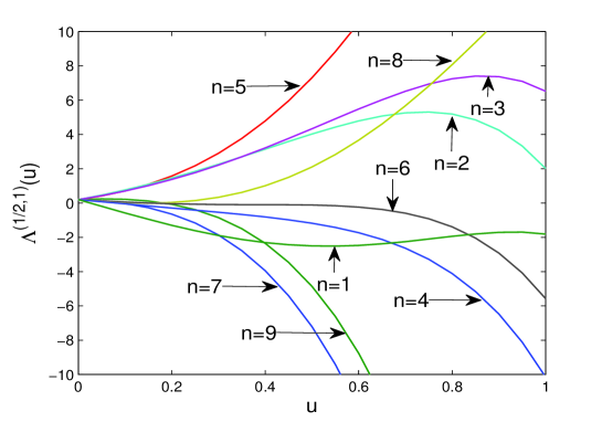
Figure 1: $\Lambda^{(\frac{1}{2},1)}(u)$ vs. $u$ calculated from both the $T-Q$ relations and exact diagonalization of $t^{(\frac{1}{2},1)}(u)$ for $N=2$, $\eta=1$, $p_{+}=0.1$, $p_{-}=0.2$, $\alpha_{+}=0.3$, $\alpha_{-}=0.4$. The correspondence is indicated by the number $n=1$ to $9$.

Numerical solutions of the BAEs and exact diagonalizations of the transfer matrix $t^{(\frac{1}{2},1)}(u)$ and the Hamiltonian (4.75) are performed for the case of $N=2$ and randomly choosing of boundary parameters. The results are listed in Table 1 for $M=0$ and Table 2 for $M=2$, respectively. The eigenvalues of the Hamiltonian obtained by solving the BAEs are exactly the same to those obtained by the exact diagonalization of the Hamiltonian. The eigenvalues $\Lambda^{(\frac{1}{2},1)}(u)$ of the transfer matrix $t^{(\frac{1}{2},1)}(u)$ are shown in Figure 1. Again, the curves of $\Lambda^{(\frac{1}{2},1)}(u)$ calculated from the BAEs and the $T-Q$ relations coincide exactly with those from the exact diagonalization of the transfer matrix $t^{(\frac{1}{2},1)}(u)$. The numerical results strongly suggest that a fixed $M$ is enough to give the complete spectrum of the transfer matrix.

5 Conclusions

The spin-$s$ XXX chain with the generic non-diagonal boundary terms specified by the most general non-diagonal $K$-matrices given by (2.21)-(2.30) has been studied by the off-diagonal Bethe anstz method. Based on the intrinsic properties of the fused $R$-matrices and $K$-matrices, we obtain the closed operator identities (3.7) of the fundamental transfer matrix $t^{(\frac{1}{2},s)}(u)$. These identities, together with other properties (3.8)-(3.10), allow us to construct an off-diagonal (or inhomogeneous) $T-Q$ equation (4.1) of the eigenvalues of the transfer matrix and the associated BAEs (4.14)-(4.15). It should be emphasized that there are a variety of forms of the inhomogeneous $T-Q$ relations such as (4.16), (4.19) and (4.22). Each of them should give the complete spectrum of the transfer matrix. Taking the spin-$1$ XXX chain as an example, we give the numerical evidence for two-site $s=1$ case. We note that the method developed in the present paper can also be applied to the integrable models with cyclic representations such as the lattice sine-Gordon model, the $\tau_{2}$ model, the relativistic Toda chain and the chiral Potts model with generic integrable boundary conditions.

For the spin-$\frac{1}{2}$ case, the Bethe states corresponding to the $T-Q$ relation (4.16) were constructed in [46] (also conjectured in [45]) with the helps of the SoV basis proposed in [31]. It is interesting that the resulting Bethe states directly induces the homogeneous limits of the SoV states constructed in [31]. Following the similar procedure, the eigenstates for the spin-$s$ open chains might be constructed with a similar basis proposed in [55].

Appendix A: Proof of the inhomogeneous $T-Q$ relation

In this appendix, we show that each solution of (3.12)-(3.17) can be parameterized in terms of the inhomogeneous $T-Q$ relation (4.1) with two fixed non-negative integers $m$ and $M$ (taking $m=M=0$ as an example).

Let us introduce a function $f(u)$ associated with each solution $\Lambda(u)$ of (3.12)-(3.17)

$$f(u)=\Lambda^{(\frac{1}{2},s)}(u)Q(u)-a^{(s)}(u)Q(u-\eta)-d^{(s)}(u)Q(u+\eta)-c\,u(u+\eta)F^{(s)}(u),$$ (A.1)

where the functions $a^{(s)}(u)$, $d^{(s)}(u)$, $F^{(s)}(u)$, $c$ and $Q(u)$ are given by (4.2)-(4.5) and (4.17) respectively. It follows from its definition that the function $f(u)$, as a function of $u$, is a polynomial of degree $2(2s+1)N+2$ with the crossing symmetry

$$f(-u-\eta)=f(u).$$ (A.2)

This very property implies that the function can be fixed by its values at $(2s+1)N+2$ different points. It is clear from the relations (3.14) and (3.15) that

$$f(0)=0,\quad{\rm and}\,\lim_{u\rightarrow\infty}f(u)=0\times u^{2(2s+1)N+2}+\ldots.$$ (A.3)

This means that it is enough to completely determine $f(u)$ by fixing its values at other $(2s+1)N$ independent points. Thanks to the fact that $Q(u)$ is also a crossing polynomial (i.e., $Q(-u-\eta)=Q(u)$) of degree $4sN$ with a known coefficient of the term $u^{4sN}$, for each solution $\Lambda(u)$ of (3.12)-(3.17) one can always choose the function $Q(u)$ of form (4.17) such that the following equations hold:

$$f(\theta_{j}+(s-\frac{1}{2}-k)\eta)=0,\quad k=0,\ldots,2s,\,{\rm and}\quad j=1,\ldots,N.$$ (A.4)

Then the relations (A.2)-(A.4) leads to $f(u)=0$ or that each solution of (3.12)-(3.17) can be parameterized in terms of the inhomogeneous $T-Q$ relation (4.16) with properly choice of the function $Q(u)$. In fact the conditions (A.4) are equivalent to the following $(2s+1)N$ linear equations with respect to the values of $Q(u)$ at the $(2s+1)N$ different points $\{\theta_{j}+(s-\frac{1}{2}-k)\eta|k=0,\ldots,2s,\,j=1,\ldots,N\}$, namely,

$$B^{(j)}\,X^{(j)}=0,\quad j=1,\ldots,N,$$ (A.5)

with each $(2s+1)\times(2s+1)$ matrix $B^{(j)}$ is given by

$$\left(\begin{array}[]{cccccc}\Lambda(\theta_{j}+(s-\frac{1}{2})\eta)&-a(\theta_{j}+(s-\frac{1}{2})\eta)&&&&\\[4.0pt] -d(\theta_{j}+(s-\frac{3}{2})\eta)&\Lambda(\theta_{j}+(s-\frac{3}{2})\eta)&-a(\theta_{j}+(s-\frac{3}{2})\eta)&&&\\[16.0pt] &\ddots&\ddots&\ddots&&\\[16.0pt] &&&-d(\theta_{j}-(s+\frac{1}{2})\eta)&\Lambda(\theta_{j}-(s+\frac{1}{2})\eta)&\end{array}\right),$$ (A.10)

and the $(2s+1)$ components vector $X^{(j)}$ is given by

$$\left(\begin{array}[]{c}Q(\theta_{j}+(s-\frac{1}{2})\eta)\\[4.0pt] Q(\theta_{j}+(s-\frac{3}{2})\eta)\\[4.0pt] \vdots\\[4.0pt] Q(\theta_{j}-(s+\frac{1}{2})\eta)\end{array}\right).$$ (A.15)

The conditions that the $(2s+1)N$ linear equations (A.5) have non-zero solutions is that the determinant of each matrix $B^{(j)}$ vanishes, namely, ${\rm Det}(B^{(j)})=0$. In this case, the number of independent linear equations (A.5) is reduced to $2sN$ and one can always fix at most the $2sN$ values (up to a scaling factor) of $Q(u)$ at $2sN$ points among $\{\theta_{j}+(s-\frac{1}{2}-k)\eta|k=0,1,\ldots,2s,\,j=1,\ldots,N\}$, for an example, $\{\theta_{j}+(s-\frac{1}{2}-k)\eta|k=1,\ldots,2s,\,j=1,\ldots,N\}$. Direct calculation shows that the vanishing of the determinants of $B^{(j)}$ are exactly the very identities (3.13). Therefore, each solution $\Lambda(u)$ of (3.12)-(3.17) allows one to parameterize it in terms of the inhomogeneous $T-Q$ relation (4.16) where $Q(u)$ can be determined either by its values at $2sN$ different points via the equations (A.5) or its roots: $\{\lambda_{j}|j=1,\ldots,2sN\}$ in (4.17) via the associated BAEs (4.18).

One can use the similar method to check that each solution of (3.12)-(3.17) can be also parameterized in terms of the inhomogeneous $T-Q$ relation with other values of $m$ and $M$. In this case the degree of the corresponding function $f(u)$ becomes $(2s+1)N+m$. Thanks to the relation (3.12)-(3.17), besides the $(2s+1)N$ conditions (A.4), one is always able to choose its values at some extra $m$ points to be zero such that the associated $T-Q$ satisfied.

References

• [1] J. Wess and B. Zumino, Phys. Lett. B 37, 95 (1971).
• [2] S. Novikov, Usp. Math. Nauk. 37, 3 (1982).
• [3] E. Witten, Commun. Math. Phys. 92, 455 (1984).
• [4] R. Thomale, S. Rachel, P. Schmitteckert and M. Greiter, Phys. Rev. B 85, 195149 (2012).
• [5] R. Shankar and E. Witten, Phys. Rev. D 17, 2134 (1978);
C. Ahn, D. Bernard and A. Leclair, Nucl. Phys. B 346, 409 (1990).
• [6] T. Inami, S. Odake and Y. -Z. Zhang, Phys. Lett. B 359, 118 (1995);
R. I. Nepomechie, Phys. Lett. B 509, 183 (2001);
Z. Bajnok, L. Palla and G. Takacs, Nucl. Phys. B 644, 509 (2002).
• [7] H. Frahm and M. Stahlsmeier, Phys. Lett. A 250, 293 (1998).
• [8] N. Andrei and C. Destri, Phys. Rev. Lett. 52, 364 (1984).
• [9] A. Tsvelik and P. Wiegmann, Z. Phys. 54, 201 (1984).
• [10] J. Dai, Y. Wang and U. Eckern, Phys. Rev. B 60, 6594 (1999).
• [11] A. B. Zamolodchikov and V. A. Fateev, Sov. J. Nucl. Phys. 32, 298 (1980).
• [12] P. P. Kulish and E. K. Sklyanin, Lecture Notes in Physics 151, 61 (Springer, 1982);
P. P. Kulish, N. Yu. Reshetikhin and E. K. Sklyanin, Lett. Math. Phys. 5, 393 (1981);
P. P. Kulish and N. Yu. Reshetikhin, J. Sov. Math. 23, 2435 (1983);
A. N. Kirillov and N. Yu. Reshetikhin, J. Sov. Math. 35, 2627 (1986);
A. N. Kirillov and N. Yu. Reshetikhin, J. Phys. A 20, 1565 (1987).
• [13] C. N. Yang, Phys. Rev. Lett. 19, 1312 (1967).
• [14] R. J. Baxter, Exactly Solved Models in Statistical Mechanics (Academic Press, London, 1982).
• [15] H. M. Babujian, Nucl. Phys. B 215, 317 (1983);
L. A. Takhtajan, Phys. Lett. A 87, 479 (1982);
H. M. Babujian, Phys. Lett. A 90, 479 (1982).
• [16] I. V. Cherednik, Theor. Math. Phys. 61, 977 (1984).
• [17] E. K. Sklyanin, J. Phys. A 21, 2375 (1988).
• [18] H. J. de Vega and A. Gonzales-Ruiz, J. Phys. A 27, 6129 (1994).
• [19] S. Ghoshal and A. B. Zamolodchikov, Int. J. Mod. Phys. A 9, 3841 (1994).
• [20] J. Cao, H. -Q. Lin, K. -J. Shi and Y. Wang, Nucl. Phys. B 663, 487 (2003).
• [21] R. I. Nepomechie, J. Phys. A 34, 9993 (2001);
R. I. Nepomechie, Nucl. Phys. B 622, 615 (2002);
R. I. Nepomechie, J. Stat. Phys. 111, 1363 (2003);
R. I. Nepomechie, J. Phys. A 37, 433 (2004).
• [22] W. -L. Yang, Y. -Z. Zhang and M. Gould, Nucl. Phys. B 698, 503 (2004).
• [23] J. de Gier and P. Pyatov, J. Stat. Mech. P03002, (2004);
A. Nichols, V. Rittenberg and J. de Gier, J. Stat. Mech. P03003, (2005);
J. de Gier, A. Nichols, P. Pyatov and V. Rittenberg, Nucl. Phys. B 729, 387 (2005).
• [24] J. de Gier and F. H. L. Essler, Phys. Rev. Lett. 95, 240601 (2005);
J. de Gier and F. H. L. Essler, J. Stat. Mech. P12011, (2006).
• [25] A. Doikou and P. P. Martins, J. Stat. Mech. P06004, (2006);
A. Doikou, J. Stat. Mech. P09010, (2006).
• [26] Z. Bajnok, J. Stat. Mech. P06010, (2006).
• [27] W. -L. Yang, R. I. Nepomechie and Y. -Z. Zhang, Phys. Lett. B 633, 664 (2006).
• [28] W. -L. Yang and Y. -Z. Zhang, Nucl. Phys. B 744, 312 (2006).
• [29] W. Galleas, Nucl. Phys. B 790, 524 (2008).
• [30] H. Frahm, A. Seel and T. Wirth, Nucl. Phys. B 802, 351 (2008).
• [31] G. Niccoli, J. Stat. Mech. P10025, (2012);
G. Niccoli, Nucl. Phys. B 870, 397 (2013);
G. Niccoli, J. Phys. A 46, 075003 (2013);
S. Faldella, N. Kitanine, G. Niccoli, J. Stat. Mech. P01011, (2014).
• [32] S. Belliard, N. Crampé, E. Ragoucy, Lett. Math. Phys. 103, 493 (2013).
• [33] L. Frappat, R. I. Nepomechie and E. Ragoncy, J. Stat. Mech. P09008, (2007).
• [34] R. Murgan, JHEP 04, 076 (2009).
• [35] R. Baiyasi and R. Murgan, J. Stat. Mech. P10003, (2012).
• [36] C.S. Melo, G.A.P. Ribeiro, M.J. Martins, Nucl. Phys. B 711 [FS], 565 (2005).
• [37] J. Cao, W. -L. Yang, K. Shi and Y. Wang, Phys. Rev. Lett. 111, 137201 (2013);
J. Cao, W. -L. Yang, K. Shi and Y. Wang, Nucl. Phys. B 875, 152 (2013);
J. Cao, S. Cui, W. -L. Yang, K. Shi and Y. Wang, Nucl. Phys. B 866, 185 (2014);
J. Cao, W. -L. Yang, K. Shi and Y. Wang, Nucl. Phys. B 877, 152 (2013).
• [38] Y. -Y. Li, J. Cao, W. -L. Yang, K. Shi and Y. Wang, Nucl. Phys. B 879, 98 (2014).
• [39] X. Zhang, J. Cao, W. -L. Yang, K. Shi and Y. Wang, J. Stat. Mech. P04031 (2014).
• [40] J. Cao, W. -L. Yang, K. Shi and Y. Wang, JHEP 04, 143 (2014).
• [41] K. Hao, G. -L. Li, W. -L. Yang, K. Shi and Y. Wang, JHEP 06, 128 (2014).
• [42] Y. -Y. Li, J. Cao, W. -L. Yang, K. Shi and Y. Wang, Nucl. Phys. B 884, 17 (2014).
• [43] P. Baseilhac and K. Koizumi, J. Stat. Mech. P09006 (2007).
• [44] N. Kitanine, J.-M. Maillet, G. Niccoli, Open spin chains with generic integrable boundaries: Baxter equation and Bethe ansatz completeness from SOV, arXiv:1401.4901.
• [45] S. Belliard and N. Crampé, SIGMA 9, 072 (2013).
• [46] X. Zhang, Y.-Y. Li, J. Cao, W. -L. Yang, K. Shi and Y. Wang, Retrieve the Bethe states of quantum integrable models solved via off-diagonal Bethe ansatz, arXiv:1407.5294v2.
• [47] L. Mezincescu, R.I. Nepomechie and V. Rittenberg, Phys. Lett. A 147, 70 (1990).
• [48] E. C. Fireman, A. Lima-Santos and W. Utiel, Nucl. Phys. B 626, 435 (2002).
• [49] A. Doikou, Nucl. Phys. B 668, 447 (2003).
• [50] T. Inami, S. Odake and Y. -Z. Zhang, Nucl. Phys. B 470, 419 (1996).
• [51] R. I. Nepomechie, J. Phys. A 46, 442002 (2013).
• [52] L. Mezincescu and R. I. Nepomechie, J. Phys. A 25, 2533 (1992);
Y.-K. Zhou, Nucl. Phys. B 458, 504 (1996).
• [53] C. Korff, J. Phys. A 41, 295206 (2008).
• [54] Y. Jiang, S. Cui, J. Cao, W. -L. Yang and Y. Wang, Completeness and Bethe root distribution of the spin-1/2 Heisenberg chain with arbitrary boundary fields, arXiv:1309.6456.
• [55] G. Niccoli, J. Math. Phys. 54, 053516 (2013).