Time-resolved charge fractionalization in inhomogeneous Luttinger liquids

Abstract

The recent observation of charge fractionalization in single Tomanga-Luttinger liquids (TLLs) [Kamata et al., Nature Nanotech., 9 177 (2014)] opens new routes for a systematic investigation of this exotic quantum phenomenon. In this Letter we perform measurements on two adjacent TLLs and put forward an accurate theoretical framework to address the experiments. The theory is based on the plasmon scattering approach and can deal with injected charge pulses of arbitrary shape in TLL regions. We accurately reproduce and interpret the time-resolved multiple fractionalization events in both single and double TLLs. The effect of inter-correlations between the two TLLs is also discussed.

Introduction.— When electrons are confined in one spatial dimension the traditional concept of Fermi-liquid quasiparticles breaks down giamarchi ; vignale ; gonzalez . The Fermi surface collapses and the elementary excitations become collective modes of bosonic nature haldane ; these are two distinctive features of the so-called Tomonaga-Luttinger liquid (TLL) tomonaga ; luttinger . A paradigmatic example of TLL is the edge state of a quantum Hall system, typically created on contiguous boundaries of 2D semiconductor heterostructures chang . Here the properties of the TLL can be tuned by varying the gate voltage kamataprb , the magnetic field, the filling factor $\nu$ chang , and electrostatic environment of the channel kumata ; hashisaka . Spatially separated TLLs with opposite chirality can be realized in systems with $\nu>1$ and, as a result of strong correlations, charge fractionalization occurs lederer ; lederer2 . According to the plasmon scattering theory safi1 ; safi2 an electron injected into a TLL region undergoes multiple reflections from one edge of the sample to the other. A fraction $r$ (dependent on the TLL parameter $g$) of the injected charge $Q$ is reflected back in the adjacent edge, and the remaining fraction $1-r$ is transmitted forward through the same edge. This fractionalization is a transient effect safi1 ; safi2 ; salvay ; psc ; iucci ; pcb ; dolcini ; oreg ; neder . Due to charge compensations occurring at every fractionalization a full charge $Q$ is transmitted in the long-time limit. Therefore, only time-resolved (or finite frequency) experiments could detect the value of the fractional charge $rQ$. The first conclusive evidence of transient fractionalization was reported only recently by means of time-resolved transport measurements of charge wave packets kamata . This provides a complementary evidence of fractionalization seen in shot-noise measurements dolcini ; oreg ; neder ; unpubl , frequency-domain experiments bocquillon , and momentum-resolved spectroscopy steinberg .

In this Letter we implement the technique developed in Ref. kamata to perform transport measurements across two spatially separated TLLs and highlight the effect of inter-TLL interactions. Furthemore we put forward a theoretical framework to calculate the evolution of wavepackets of arbitrary shape scattering against multiple noninteracting-liquid/TLL interfaces arranged in different geometries. By a proper treatment of the boundary conditions we are able to make direct comparisons with the measured signal. All features of the transient current are correctly captured both in the single and double TLL systems.

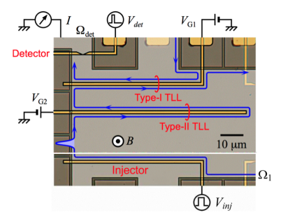
Figure 1: Optical micrograph of the sample (the horizontal white line indicates that unused parts are not shown). Metal gate electrodes (gold regions) are patterned on a 2DES (light grey region) and etched insulating GaAs (dark grey regions). The 2DES located $90\,\mathrm{nm}$ below the surface has a density of $1.45\times 10^{11}\,\mathrm{cm}^{-2}$ and a low-temperature mobility of $4.0\times 10^{5}\,\mathrm{cm}^{2}\mathrm{V}^{-1}\mathrm{s}^{-1}$. Chiral one-dimensional edge channels are formed along the edge of the 2DES in a strong perpendicular magnetic field $B=4.0\,\mathrm{T}$, which corresponds to a bulk filling factor $\nu=1.5$. Type-I and Type-II TLL regions has an effective length of $\ell_{1}=68$ and $\ell_{2}=80\,\mu\mathrm{m}$, respectively, and a width of $1\,\mu\mathrm{m}$. The charge wavepacket is injected at the falling edge of a voltage step $5\,\mathrm{mV}$ in amplitude applied to an injection gate $V_{\mathrm{inj}}$. The QPC detector is set at the pinched-off regime, and one of the gate voltages is modulated by a voltage pulse $V_{\mathrm{det}}$ of height $0.2\mathrm{V}$ for a period of $80\,\mathrm{ps}$ to temporally enhance the transmission probability of the QPC. The average current $I$ through the QPC as a function of time interval $t$ between two voltage pulses is measured at the detection Ohmic contact $\Omega_{\mathrm{det}}$ under the pulse pattern repeated at $25\,\mathrm{MHz}$. All measurements were carried out at $\sim 300\,\mathrm{mK}$.

Experimental setup.— Figure 1 shows the sample patterned on a GaAs/AlGaAs heterostructure with chiral one-dimensional edge channels formed along the edge of the two-dimensional electronic system (2DES) in a strong perpendicular magnetic field $B$. Artificial TLL can be formed in a pair of counter-propagating edge channels along both sides of a narrow gate metal kamata . Other unpaired channels are considered as noninteracting (NI) leads. Two types of TLL regions were investigated: Type-I TLL, with NI leads on both ends, and Type-II TLL, with NI leads only on the left and a closed end on the right. We can selectively activate one or both the TLL regions by applying appropriate voltages ($V_{G1}$ and $V_{G2}$). A non-equilibrium charge wavepacket of charge $Q\simeq 150\;e$ is generated by depleting electrons around an injection gate with a voltage step applied on the gate. The wavepacket travels along a NI lead as shown in Fig. 1, and undergoes charge fractionalization processes at the left and right ends of the TLL regions. The multiple charge fractionalization processes must be investigated separately. The reflected wavepacket appears on another NI lead, on which time-resolved charge detection scheme is applied with a quantum point contact (QPC) detector kamataprb . We have successfully resolved the reflected wavepackets of charge $Q^{(\mathrm{refl})}_{1}$ fractionalized at the left boundary and $Q^{(\mathrm{refl})}_{2}$ at the right boundary. Typical waveforms are shown by dots in Figs. 3 and 4. The fractionalization ratio $r$, which is related to the TLL parameter $g$ through $g=(1-r)/(1+r)$, can be extracted from $r=Q^{(\mathrm{refl})}_{1}/Q$ and is found to be approximately $g=0.92$kamata . The charge velocity in the TLL region can be measured from the time interval between the two reflected wavepackets. The interest in activating both Type-I and -II regions is to assess the role of the long-range Coulomb interaction between the two TLLs.

Model and formalism.—

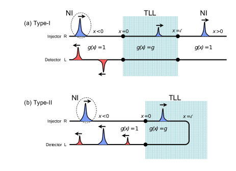
Figure 2: (Color online) Model of the experimental setup. The wavepacket is injected from the $R$ edge (dashed circle). The figure shows a snapshot of the fractionalized charge when the injected wavepacket has passed the TLL region. Transmitted packets are dark (blue) and reflected packets are light (red). Type-I geometry (a): $R$ and $L$ edges with NI regions for $x<0$ and $x>\ell$, and activated TLL region for $0<x<\ell$. Type-II geometry (b): a single bent edge with NI regions for $x<0$, and activated TLL region for $0<x<\ell$.

To model the setup of Fig. 1 we consider two parallel chiral edges hosting Right ($R$) and Left ($L$) moving electrons, see Fig. 2. Electrons with opposite chirality experience a space-dependent repulsion $V(x)$. In the regions where $V(x)=0$ we have a NI liquid and otherwise, $V(x)=V$, a TLL is formed. For electrons with the same chirality an additional repulsion $U(x)=U$ in the NI liquid and $U(x)=U^{\ast}$ in the TLL is included. Spatial inhomogeneities in $V(x)$ induce back-scattering from the $R$ to the $L$ edge (and vice versa) even without a inter-edge hopping safi1 ; safi2 . The low-energy Hamiltonian of the system reads changRMP

$$\hat{H}\! = \!\sum_{\alpha=L,R}i\alpha v_{F}\int dx\,\hat{\psi}^{\dagger}_{\alpha}(x)\partial_{x}\hat{\psi}_{\alpha}(x)$$ (1)

$$+ \!2\pi\!\!\int\!dx\left\{\!V(x)\,\hat{n}_{R}(x)\hat{n}_{L}(x)+\frac{U(x)}{2}\left[\hat{n}^{2}_{R}(x)+\hat{n}^{2}_{L}(x)\right]\!\right\}\quad\;$$

where the fermion field $\hat{\psi}^{(\dagger)}_{R/L}$ destroys (creates) $R/L$ edge-state electrons moving with bare Fermi velocity $\alpha v_{F}\equiv\pm v_{F}$, and $\hat{n}_{\alpha}\equiv\,\,:\hat{\psi}^{\dagger}_{\alpha}\hat{\psi}_{\alpha}:$ is the density fluctuation operator. For a nonperturbative treatment of the interaction we bosonize the field operators as $\hat{\psi}_{\alpha}(x)=\frac{\eta_{\alpha}}{\sqrt{2\pi a}}e^{-2\sqrt{\pi}\,i\hat{\phi}_{\alpha}(x)},$ with $\eta_{\alpha}$ the anticommuting Klein factor, $a$ a short-distance cutoff, and $\hat{\phi}_{\alpha}(x)$ the chiral boson fields. The density can then be expressed as $\hat{n}_{\alpha}=-\partial_{x}\hat{\phi}_{\alpha}/\sqrt{\pi}.$ By introducing the auxiliary fields $\hat{\phi}=\hat{\phi}_{L}+\hat{\phi}_{R}$ and $\hat{\theta}=\hat{\phi}_{L}-\hat{\phi}_{R}$ Eq. (1) becomes giamarchi

$$\hat{H}=\frac{1}{2}\int dx\left\{\frac{v(x)}{g(x)}[\partial_{x}\hat{\phi}(x)]^{2}+v(x)g(x)[\partial_{x}\hat{\theta}(x)]^{2}\right\},$$ (2)

where for a TLL region of length $\ell$ the parameter $g(x)$ and the renormalized velocity $v(x)$ depends on the interactions through the relations

$$g(x) = \left\{\begin{array}[]{ccc}\sqrt{\frac{v_{F}+U^{*}-V}{v_{F}+U^{*}+V}}\equiv g&&\mathrm{for}\quad 0<x<\ell\\ 1&&\mathrm{otherwise}\\ \end{array}\right.$$ (5)

$$v(x) = \left\{\begin{array}[]{ccc}\sqrt{(v_{F}+U^{*})^{2}-V^{2}}\equiv v^{*}&&\mathrm{for}\quad 0<x<\ell\\ v_{F}+U\equiv v&&\mathrm{otherwise.}\\ \end{array}\right.$$

The temporal evolution of the system is governed by the equation of motion for $\hat{\phi}$ suppmat . Taking the average $\phi(x,t)\equiv\langle\hat{\phi}(x,t)\rangle$ over an arbitrary wavepacket state we find

$$\frac{d^{2}}{dt^{2}}\phi(x,t)=v(x)g(x)\partial_{x}\left(\frac{v(x)}{g(x)}\partial_{x}\phi(x,t)\right),$$ (9)

which implies that $\phi$ and $\frac{v(x)}{g(x)}\partial_{x}\phi$ are continuous for all $x$. For independent channels, as those of the Type-I geometry illustrated in Fig. 2, these are the only conditions to impose on the solution of Eq. (9) safi1 ; hashisaka ; HRHL.2011 . On the other hand, for the Type-II geometry one has to further impose that $R$ electrons are converted into $L$ electrons and viceversa, i.e., that the channels are not independent. The proper treatment of boundary conditions, absent in previous works, leads to a qualitative different transient fractionalization since the transmission and reflection coefficients are entangled. Once $\phi(x,t)$ is known the total density and current are extracted from $\rho(x,t)=e\langle\hat{n}(x,t)\rangle=-e\partial_{x}\phi(x,t)/\sqrt{\pi}$ and $j(x,t)=e\partial_{t}\phi(x,t)/\sqrt{\pi}$.

We consider an incident wavepacket injected in the upper $R$ edge, see Fig. 2. Then the solution of Eq. (9) can be expanded in right-going scattering states $s_{q}(x)$ of energy $\epsilon_{q}=vq$ according to $\phi(x,t)=\int_{-\infty}^{\infty}\frac{dq}{2\pi}\phi_{q}s_{q}(x)e^{-i\epsilon_{q}t}$ bcnote . For a wavepacket initially, say at time $t=0$, localized in $x<0$ the function $\phi_{q}$ is related to the Fourier transform $\rho^{(\mathrm{inc})}_{q}$ of $\rho^{(\mathrm{inc})}(x)=\rho(x,0)$ by the relation $\phi_{q}=\frac{i\sqrt{\pi}}{eq}\rho^{(\mathrm{inc})}_{q}$ nontrivial . Therefore, once $s_{q}(x)$ is known the time-dependent density and current are given by

$$\rho(x,t) = -i\int_{-\infty}^{\infty}\frac{dq}{2\pi}\frac{\rho^{(\mathrm{inc})}_{q}}{q}e^{-i\epsilon_{q}t}\partial_{x}s_{q}(x),$$

$$j(x,t) = v\int_{-\infty}^{\infty}\frac{dq}{2\pi}\rho^{(\mathrm{inc})}_{q}e^{-i\epsilon_{q}t}s_{q}(x).$$ (10)

Below we solve the scattering problem in the geometries of the experiment.

Type-I geometry.— This geometry is illustrated in Fig. 2.a and has been realized in Ref. kamata . We look for scattering states of the form

$$s_{q}(x)=\left\{\begin{array}[]{ccc}e^{iqx}+r_{q}e^{-iqx}&\quad\mathrm{for}&\quad x<0\\ a_{q}e^{iq^{\prime}x}+b_{q}e^{-iq^{\prime}x}&\quad\mathrm{for}&\quad 0<x<\ell\\ t_{q}e^{iqx}&\quad\mathrm{for}&\quad x>\ell\,,\end{array}\right.$$ (11)

with $q^{\prime}=\frac{v}{v^{*}}q$. By imposing the continuity conditions at the boundaries we obtain a $4\times 4$ linear system suppmat that we solve exactly. If we are interested in the current detected at the collector (located in $x<0$) only the reflection coefficient $r_{q}$ is needed nota2 :

$$r_{q}=-r+4g\sum_{n=1}^{\infty}\zeta_{n}e^{2inq^{\prime}\ell},$$ (12)

where $g_{\pm}=1\pm g$, $r=\frac{g_{-}}{g_{+}}$, and $\zeta_{n}=\frac{g_{-}^{2n-1}}{g_{+}^{2n+1}}$. Inserting this expression in Eq. (10) the time-dependent density and current for $x<0$ read

$$\rho(x,t) = \rho^{(\mathrm{inc})}(x_{-})+\rho^{(\mathrm{refl})}(x_{+})$$

$$j(x,t) = v[\rho^{(\mathrm{inc})}(x_{-})-\rho^{(\mathrm{refl})}(x_{+})],$$ (13)

with $x_{\pm}=x\pm vt$, $x_{n}=\frac{2n\ell v}{v^{*}}$, and

$$\rho^{(\mathrm{refl})}(x_{+})=r\rho^{(\mathrm{inc})}(-x_{+})-4g\sum_{n=1}^{\infty}\zeta_{n}\rho^{(\mathrm{inc})}(-x_{+}+x_{n}).$$ (14)

Equation (14) generalizes the result of Ref. safi1 to arbitrary wavepacket shapes. The first reflection occurs at time $t_{1}=|x_{0}|/v$ ($x_{0}<0$ being the initial position of the wavepacket) at the left boundary and a fractionalized charge $Q^{(\mathrm{refl})}_{1}=rQ$ is reflected back in the $L$ edge (here $Q=\int dx\rho^{(\mathrm{inc})}(x)$). The transmitted fractional charge propagates in the TLL region, a second reflection occurs at the right boundary and at time $t_{2}=t_{1}+2\ell/v^{*}$ a second wavepacket of charge $Q^{(\mathrm{refl})}_{2}=-Q(4gg_{-}/g_{+}^{3})=-Qr(1-r^{2})$ appears in the $L$ edge. The fractionalization sequence continues ad infinitum and the reflected charge $Q^{(\mathrm{refl})}_{n}$ diminishes at each event. At the end of the infinite sequence the total reflected charge vanishes since $Q^{(\mathrm{refl})}=\sum_{n=1}^{\infty}Q^{(\mathrm{refl})}_{n}=-r-4g\sum_{n=1}^{\infty}\zeta_{n}=0$. This is a consequence of the chiral charge conservation and highlights the transient nature of the fractionalization phenomenon.

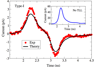
Figure 3: Type-I geometry: Calculated current (black curve) from Eqs. (13,14) versus measured current (dotted-red curve) from Ref. kamata . The inset shows the incident waveform $v\rho^{(\mathrm{inc})}$.

For the comparison with the experiment we acquire $\rho^{(\mathrm{inc})}(x_{0}-vt)$ from Ref. kamata, , see inset in Fig. 3 and used $g=0.92$, $\ell=\ell_{1}=68$ $\mu$m, $v^{*}=150$ km/s and estimated $v$ by a best fitting. As shown in Fig. 3 the agreement with the current calculated from Eq. (13) is remarkably good.

Type-II geometry.— Here a single edge is bent on itself as illustrated in Fig. 2.b. Therefore $R$ electrons in the upper branch are converted in $L$ electrons in the lower branch. We model this geometry by imposing that the $L$ amplitude $b_{q}$ of the scattering state in the TLL region equals $-a_{q}e^{2iq^{\prime}\ell}$ suppmat . Following the same line of reasoning as before we find the reflection coefficient

$$r_{q}=-r+4g\sum_{n=1}^{\infty}\xi_{n}e^{2inq^{\prime}\ell},$$ (15)

with $\xi_{n}=(-1)^{n}\frac{g_{-}^{n-1}}{g_{+}^{n+1}}$. We observe that $|r_{q}|=1$ as it should due to charge conservation. The density and current at the collector in $x<0$ are still given by Eq. (13) but the reflected density reads

$$\rho^{(\mathrm{refl})}(x_{+})=r\rho^{(\mathrm{inc})}(-x_{+})-4g\sum_{n=1}^{\infty}\xi_{n}\rho^{(\mathrm{inc})}(-x_{+}+x_{n}).$$ (16)

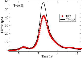
Figure 4: Type-II geometry: Calculated current (black curve) from Eqs. (13,16) versus measured current (dotted-red curve) from Ref. kamata .

In Fig. 4 we show the calculated (black curve) and measured kamata (dotted-red curve) current in the lower branch. The parameters are the same as in Fig. 3 with the only difference that $\ell=\ell_{2}=80$ $\mu$m. Again a good agreement between theory and experiment is found. The theory reproduces a small first reflection of charge $rQ$ (occurring at time $t_{1}$) and a subsequent large transmitted charge $(4g/g_{+}^{2})Q$ (occurring at time $t_{2}$).

Type-I + Type-II geometry.— Finally we present numerical and experimental results when both Type-I and Type-II TLLs are activated. As illustrated in Fig. 1 the wavepacket injected into TLL-II is partially transmitted toward TLL-I and the resulting reflected wavepacket is then measured at the collector. The measured signal is displayed in Fig. 5 (dotted red curve). The simultaneous activation of TLL-I and TLL-II produces a richer current pattern characterized by an additional peak and dip. These extra structures are naturally interpreted within our theory. The reflected wavepacket is given by $\rho^{(\mathrm{refl})}(x_{+})$ with only TLL-I activated by replacing $\rho^{(\mathrm{inc})}(x)$ in Eq. (13) with the outcome $\rho(x_{-})$ obtained by a preliminary calculation with only TLL-II activated. TLL-II alone produces a waveform similar to the incident one, with the addition of a small side peak of weight $r$ on the left, see Fig. 4. The temporal delay between the peaks is $\Delta t_{II}=2\ell_{2}/v^{*}_{II}$, where $v^{*}_{II}$ is the renormalized velocity inside TLL-II. When this double-peaked wavepacket enters TLL-I the reflected current displays a first replica of the incident shape with positive weight $r$ and a second replica of the incident shape with negative weight $-r(1-r^{2})$, as we demonstrated in Fig. 3. The delay between the two replicas is $\Delta t_{I}=2\ell_{1}/v^{*}_{I}$, $v^{*}_{I}$ being the renormalized velocity inside TLL-I. This explains the experimentally observed pattern of Fig. 5 (the inset shows a cartoon of this double fractionalization process).

The calculated reflected current is shown in Fig. 5 for comparison. From $\Delta t_{I(II)}=\ell_{1(2)}/v^{*}_{I(II)}$ with $\Delta t_{I}\approx 1.0$ ns and $\Delta t_{II}\approx 0.5$ ns we estimated $v^{*}_{I}\approx 136$ km/s, $v^{*}_{II}\approx 320$ km/s, and $v$ by a best fitting. The value $g=0.92$ (black-dashed curve) is probably too large as the additional peak and dip are almost invisible. We therefore repeated the calculation with $g=0.87$ (black-solid curve) to match the height of the positive main peak and found that the additional peak and dip are correctly more pronounced. The physical justification of a smaller $g$ is elaborated in the conclusions.

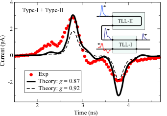
Figure 5: Measured current (dotted-red curve) from TLL-I when both TLL-I and TLL-II are activated versus calculated current with $g=0.92$ (black-dashed curve) and $g=0.87$ (black-solid curve). The inset shows a cartoon of the fractionalization process. The velocities in TLL-I and TLL-II are different (with $V_{G1}=-0.19\,\mathrm{V}$ and $V_{G2}=-1.4\,\mathrm{V}$) in order to isolate four fractionalized wavepackets.

Conclusions.— We extended the plasmon scattering approach to address the charge fractionalization phenomenon recently observed in artificial TLLs of different geometries kamata . The method allows us to monitor the temporal evolution of a charge wavepacket in each chiral edge of the experimental setup, thus providing a tool for a direct comparison with the time-resolved transport measurement. Quantitative agreement between theory and experiment is obtained for the Type-I and Type-II geometries. We then performed new measurements in a double-TLL geometry and found indications that electron correlations are enhanced due to the repulsion between electrons in different TLLs. Our calculations neglect the inter-TLL repulsion and the enhancement of correlations is effectively accounted for by a reduced TLL parameter $g$. The proper inclusion of the long-range interaction across the bulk 2DEG is eventually required for the ultimate understanding of the transport properties of interacting edge channels.

E.P. and G.S. acknowledge funding by MIUR FIRB grant No. RBFR12SW0J. H.K. and T.F. acknowledge funding by JSPS KAKENHI (21000004, 11J09248). We also thank N. Kumada, M. Hashisaka, and K. Muraki for experimental supports.

References

- (1) T. Giamarchi, Quantum Physics in One Dimension (Clarendon, Oxford, 2004).
- (2) G. Giuliani and G. Vignale, Qunatum theory of the electron liquid (Cambridge University Press, 2008).
- (3) J. González, M. A. Martín-Delgado, G. Sierra, and M. A. H. Vozmediano, Quantum Electron Liquids and High-Tc Superconductivity (Springer-Verlag, Berlin, 1995).
- (4) F.D.M. Haldane, J. Phys. C: Solid State Phys. 14, 2585 (1981).
- (5) S. Tomonaga, Prog. Theor. Phys. 5, 544 (1950).
- (6) J.M. Luttinger, J. Math. Phys. 4, 1154 (1963).
- (7) A.M. Chang, Rev. Mod. Phys. 75, 1449 (2003).
- (8) H. Kamata, T. Ota, K. Muraki, and T. Fujisawa, Phys. Rev. B 81, 085329 (2010).
- (9) N. Kumada, H. Kamata, and T. Fujisawa, Phys. Rev. B 84, 045314 (2011).
- (10) M. Hashisaka, H. Kamata, N. Kumada, K. Washio, R. Murata, K, Muraki, and T. Fujisawa, Phys. Rev. B 88, 235409 (2013).
- (11) K.-V. Pham, M. Gabay, and P. Lederer, Phys. Rev. B 61, 16397 (2000).
- (12) K.-I. Imura, K.-V. Pham, P. Lederer, and F. Piéchon, Phys. Rev. B 66, 035313 (2002).
- (13) I. Safi and H. J. Schulz, Phys. Rev. B 52, R17040 (1995).
- (14) I. Safi, Ann. Phys. (Paris) 22, 463 (1997).
- (15) M.J. Salvay, H.A. Aita, and C.M. Naón, Phys. Rev. B 81, 125406 (2010).
- (16) E. Perfetto, G. Stefanucci, and M. Cini, Phys. Rev. Lett. 105, 156802 (2010).
- (17) M.J. Salvay, A. Iucci, and C.M. Naón, Phys. Rev. B 84, 075482 (2011).
- (18) E. Perfetto, M. Cini, and S. Bellucci, Phys. Rev. B 87, 035412 (2013).
- (19) H. Kamata, N. Kumada, M. Hashisaka, K. Muraki, and T. Fujisawa, Nature Nanotech., 9 177 (2014).
- (20) B. Trauzettel, I. Safi, F. Dolcini, and H. Grabert, Phys. Rev. Lett. 92, 226405 (2004).
- (21) E. Berg, Y. Oreg, E.-A. Kim, and F. von Oppen, Phys. Rev. Lett. 102, 236402 (2009).
- (22) I. Neder, Phys. Rev. Lett. 108, 186404 (2012).
- (23) H. Inoue, A. Grivnin, N. Ofek, I. Neder, M. Heiblum, V. Umansky and D. Mahalu, arXiv1310.0691 (2013).
- (24) E. Bocquillon, V. Freulon, J. M. Berroir, P. Degiovanni, B. Pla ais, A. Cavanna, Y. Jin, and G. F ve, Nat Commun 4, 1839 (2013).
- (25) H. Steinberg, G. Barak, A. Yacoby, L. N. Pfeiffer, K. W. West, B. I. Halperin, and K. Le Hur, Nat Phys 4, 116 (2008).
- (26) A. M. Chang, Rev. Mod. Phys. 75, 1449 (2003).
- (27) See Supplemental Material at [URL will be inserted by publisher].
- (28) M. Horsdal, M. Rypestøl, H. Hansson and J. M. Leinaas, Phys. Rev. B 84, 115313 (2011).
- (29) For an incident wavepacket injected from in the lower edge .
- (30) The property that the expansion coefficients of are the same in the scattering-state basis and in the plane-wave basis is crucial to perform the -integral in Eqs. (10). This property can be checked by calculating for all , see Ref. suppmat, .
- (31) Within our convention the current carried by an excess of left-moving electrons is negative. Thus in order to compare the theoretical results with the experiment in Ref. kamata, , in producing the plots we have to revert the “” sign appearing in the second lines of Eqs. (13).
- (32) To evaluate and in the expressions of and are needed suppmat .