A Superbubble Feedback Model for Galaxy Simulations

Abstract

We present a new stellar feedback model that reproduces superbubbles. Superbubbles from clustered young stars evolve quite differently to individual supernovae and are substantially more efficient at generating gas motions. The essential new components of the model are thermal conduction, sub-grid evaporation and a sub-grid multi-phase treatment for cases where the simulation mass resolution is insufficient to model the early stages of the superbubble. The multi-phase stage is short compared to superbubble lifetimes. Thermal conduction physically regulates the hot gas mass without requiring a free parameter. Accurately following the hot component naturally avoids overcooling. Prior approaches tend to heat too much mass, leaving the hot ISM below $10^{6}$ K and susceptible to rapid cooling unless ad-hoc fixes were used. The hot phase also allows feedback energy to correctly accumulate from multiple, clustered sources, including stellar winds and supernovae.

We employ high-resolution simulations of a single star cluster to show the model is insensitive to numerical resolution, unresolved ISM structure and suppression of conduction by magnetic fields. We also simulate a Milky Way analog and a dwarf galaxy. Both galaxies show regulated star formation and produce strong outflows.

1 Introduction

Galaxies are star factories: with their large potential wells, they accrete gas and convert that gas into stars. The throttle for this process is the energy released from these stars through winds and supernovae: stellar feedback. Without this large source of energy ($\sim 3\times 10^{38}$ erg s^-1 per solar mass of stars) to stir and heat the interstellar medium, star formation would consume all available gas for every galaxy in less than a Hubble time. Not only does stellar feedback allow star formation to self-regulate, it is one of the most important processes in producing a multiphase ISM (McKee & Ostriker, 1977). A third way feedback shapes the history and structure of gas in a galaxy is by cycling (and even ejecting) gas through outflows. Galactic winds can remove potential star-forming gas from a galaxy by propelling it out of a galaxy faster than the escape velocity. Gas ‘fountains’ can reduce the cold gas available in a galactic disc by cycling it between the disc and high in the galactic halo. This acts to temporarily store gas in a reservoir above the galactic plane, where it is too hot and diffuse to form stars. These outflows are likely an important component in determining the ultimate fate of a galaxy, and are the most plausible mechanism for metal enrichment observed in the circumgalactic medium (Songaila & Cowie, 1996; Davé et al., 1998).

Much work has been done to build feedback models based on the evolution of individual supernova blastwaves (e.g. Stinson et al., 2006), but these efforts have overlooked two key factors. First, star formation is clustered; new stars are spatially and temporally correlated, and feedback from their individual winds and supernovae merge, thermalize and grow as a superbubble rather than a series of isolated supernovae. Second, because superbubbles have both hot gas $>10^{6}\;\mathrm{K}$ and sharp temperature gradients, thermal conduction is significant (Weaver et al., 1977). Omitting this process can cause one to incorrectly estimate the interior density (and thus the amount of hot gas) of superbubbles by orders of magnitude, regardless of whether or not one can resolve the superbubble. In simulations of galaxy evolution, the temporal resolution required to resolve the pre-thermalization Sedov phase is out of reach (on the order of $100\;\mathrm{yr}$), and even the post-thermalization early superbubble can require shorter timesteps than are practical. Worse still, during this period the amount of mass contained within the hot, rarefied interior of a superbubble is less than the mass of the progenitor star cluster. This can make it impossible to spatially resolve this stage in simulations where resolution elements are comparable in mass to star particles. This leads to denser, cooler feedback regions. These overcool and lead to ineffective feedback overall (Katz, 1992).

A number of approaches exist to attack the problem of overcooling. The earliest techniques were to simply deposit a fraction of the energy released in feedback events as kinetic energy (Navarro & White (1993), Mihos & Hernquist (1994), Dubois & Teyssier (2008), etc.). Gerritsen (1997) detailed a second approach; by introducing cooling shutoff, where feedback-heated gas is explicitly prevented from cooling radiatively, and Thacker & Couchman (2000) explored a range of different times for this shutoff period. Stinson et al. (2006) proposed using the time required to resolve a Sedov-Taylor blastwave, and showed that this can be an effective way of modelling feedback in cosmological simulations of galaxy evolution. Agertz et al. (2013) used a decaying non-cooling energy, where energy in a non-cooling state decayed back to the ‘normal’ cooling form. Another technique is to manually decouple density estimates and hydrodynamic interactions between feedback-heated gas and the cold ISM (Marri & White (2003), Scannapieco et al. (2006), etc.). With extremely high resolution, it is possible to generate rarefied hot gas from feedback directly without a subgrid treatment (e.g. Hopkins, Quataert & Murray, 2012). However, as we argue here, mass transfer between hot and cold gas depends on the physics of conduction which relies on sub-parsec gradients. These are beyond the reach of even the highest resolution galaxy scale simulations so some subgrid modeling may be unavoidable.

Another approach has been to explicitly model the multiphase ISM below the resolution limit. Springel & Hernquist (2003) described a multiphase model based on the theoretical framework of McKee & Ostriker (1977). Each particle was composed of an isobaric mix of cold clouds and ambient warm to hot gas. Radiative cooling coverts warmer gas into cold. The cold phase forms stars on a characteristic timescale chosen to yield a Schmidt-type star formation law. An empirical model of stellar feedback evaporates the cold phase. Springel & Hernquist (2003) recognized that while this model works well for simulating star formation and feedback in quiescent galaxies, the coupling of hot and cold mass can prevent hot gas from leaving the disc as winds or outflows. Their solution was to convert a fraction of the feedback energy in a kinetic kick on selected particles, in the same vein as Mihos & Hernquist (1994).

Both Dalla Vecchia & Schaye (2012) and Hopkins, Quataert & Murray (2012) have shown that it is possible to get consistent wind results for a given energy input model. Dalla Vecchia & Schaye (2012) demonstrated that simply depositing energy stochastically to ensure a constant temperature increase for feedback-heated gas can directly generate winds. They found that for the same feedback energy, changing the temperature of feedback-heated gas results in significant differences in both star formation regulation and galactic outflows. Higher feedback temperatures, $\Delta T>10^{7}\;\mathrm{K}$, avoid overcooling and allow for more efficient regulation and higher velocity galactic winds. This still leaves open the question of what sets this temperature? This question is equivalent to asking: what sets the mass-loading in stellar feedback? Previous feedback models have not explored key physical mechanisms, such as conduction, that affect mass-loading.

The above sub-grid models are reasonably successful at preventing overcooling. However, many of them have limitations which are increasingly severe with improving resolution. For example, stellar feedback in the form of kinetic energy is rapidly converted into thermal energy as it encounters the ISM and shocks (Durier & Dalla Vecchia, 2012). In nature, the gas heated by feedback doesn’t completely stop cooling radiatively, it merely cools inefficiently. Applying a cooling shutoff is unlikely to give the correct behaviour in different star forming environments and is also dependent on the integrated energy injection from all nearby stars. Finally, because star formation is clustered, feedback is localized within starforming regions.

Recent studies such as Nath & Shchekinov (2013) and Sharma et al. (2014) have emphasized that feedback from clustered stars forms superbubbles, which behave quite differently from isolated supernovae. A key outcome is that superbubbles are intrinsically more efficient than individual supernovae at converting feedback energy into gas motions, particularly at late times and over larger scales. The reason for this difference is that gas heated by feedback remains distinct from the cooler surrounding material. Most current models smear together the hot bubble with the cold shell surrounding it. This results in an intermediate effective temperature that is prone to overcooling. Separating the hot and cold phases automatically avoids overcooling. Dalla Vecchia & Schaye (2012) achieved this with a stochastic feedback model. An alternative approach is to add an explicit hot reservoir to accumulate feedback mass and energy. This avoids overcooling without artificially turning off cooling and correctly handles feedback from multiple sources over time without resorting to a stochastic approach. Such a model still leaves the bubble mass as a free parameter. Mac Low & McCray (1988) showed that thermal conduction controls the mass flow into the hot bubble from the cold shell. This evaporation process regulates the temperature of the hot bubble and determines how much mass is heated by feedback. Adding a sub-grid model for evaporation allows the physics of thermal conduction to set bubble temperatures and masses.

Drawing on these facts, we can construct a superbubble-based feedback model. As outlined in Mac Low & McCray (1988), superbubbles efficiently convert feedback energy into thermal energy in a hot phase and kinetic energy in an expanding cold shell. The rarefied hot phase cools inefficiently, avoiding overcooling. Thus a correct model requires following distinct hot and cold phases even when they may be difficult to resolve directly. A new requirement with respect to prior feedback models is the inclusion of thermal conduction. Conduction both smooths the temperature distribution in the hot gas and mediates mass flows where hot gas meets a cold phase. Thus a second feature of such a model is that an explicit physical process sets the amount of hot gas in the ISM and in outflows.

In this paper, we begin by explaining the theoretical underpinning and numerical implementation of the superbubble-based feedback method in section 2. In section 3.1 we use a single star cluster to illustrate the effectiveness of our model at capturing the basic behaviour of superbubbles at high and low resolution. In section 3.2 we apply the model to simulations of isolated galaxies to explore the impact on the galaxy scale ISM and the production of outflows.

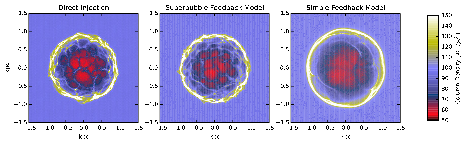
Figure 1: Column density projections from the simulations of a single star cluster with mass $3\times 10^{4}\;\mathrm{M_{\odot}}$, $50\;\mathrm{Myr}$ after the cluster has formed. The superbubble feedback model (center column) produces bubbles with radius and enclosed mass that match well to the direct injection simulations (left column). This is shown quantitatively in figure 2 and figure 6. The simple model (right column), despite injecting the same amount of energy, fails to generate enough hot mass inside the bubble, and subsequently suppresses the growth of Vishniac instabilities along the bubble edge because of the poorly resolved hot interior.

2 Thermal Conduction and Feedback Method

Our new treatment of feedback has three components. The first is the addition of thermal conduction. Inside resolved hot bubbles, thermal conduction maintains uniform temperatures. In the presence of strong gradients, thermal conduction can lead to evaporative mass flows from cold to hot gas. The second component is a stochastic model of evaporation to allow resolved hot gas to continue to gain mass from nearby cold gas. Thus, the amount of cold gas heated by feedback is not a free parameter, but is set by thermal conduction. Without a mechanism like thermal conduction, this hot gas mass is set by how many fluid elements have feedback energy deposited into them. It is important to note that in our model these processes operate everywhere temperatures are above $10^{5}K$.

Finally, in the first few $\mathrm{Myr}$ of feedback heating, the mass contained within a hot bubble can be smaller than the simulation gas mass resolution. To prevent overcooling, we allow resolution elements to become briefly two-phase; a hot interior (bubble) in contact with a cold shell. Evaporation of the cold shell moderates this two-phase period, rapidly returning particles to single phase once their cold phase has been fully evaporated. Our model does not assume all fluid elements are multiphase, but only those in which a partial feedback region exists. This allows the model to follow winds and outflows without continuing to rely on sub-grid machinery.

Young stellar population steadily release energy in the form of winds and SNe at a rate of $3\times 10^{38}\;\mathrm{erg\;s^{-1}M_{\odot}^{-1}}$ for around 40 Myr (Leitherer et al., 1999). We deposit this energy into the gas particle nearest to the star particle. In following with past work, we use the feedback rates and times for supernovae, but the method is general enough to handle heating from stellar winds, ionization, etc. Heating takes effect $4\;\mathrm{Myr}$ after a star forms, and continues until $30\;\mathrm{Myr}$ after the star particle forms (the time associated with SNII from OB stars). Thus, each supernova releases $10^{51}\;\mathrm{erg}$, and each star particle will release $10^{49}\;\mathrm{ergM^{-1}_{\odot}}$ using the Chabrier (2003) IMF.

2.1 Thermal Conduction

In an ionized gas, thermal conduction, mediated by electrons, transports heat down temperature gradients. This flux, $\mathbf{Q}=-\kappa\nabla T$, depends on the temperature gradient and the conduction coefficient, as derived by Cowie & McKee (1977),

$$\kappa(T)=1.8\left(\frac{2}{\pi}\right)^{3/2}\frac{T^{5/2}k_{B}^{7/2}}{m_{e}\,e^{4}\ln\Lambda}.$$ (1)

This coefficient depends only on the Coulomb logarithm $\ln\Lambda$ (which has an extremely weak dependence on density), and is well approximated by $\kappa(T)=\kappa_{0}\,T^{5/2}$, where $\kappa_{0}$ is $6.1\times 10^{-7}\;\mathrm{erg\;s^{-1}K^{-7/2}cm^{-1}}$ in the absence of magnetic fields. In order for this situation to not cause spontaneous currents, a corresponding mass flux, in the opposite direction, must also occur (Cowie & McKee, 1977). With spherical symmetry, this implies a mass flow rate that depends on the sound speed in the hot gas, $c_{\rm s}$, as follows,

$$\frac{5}{2}\dot{M}c_{\rm s}^{2}=4\,\pi^{2}r^{2}\kappa(T)\frac{{\rm d}T}{{\rm d}r}.$$ (2)

These rates hold only when the mean free path of electrons in the medium is smaller than the scale length of the temperature gradient. If the gradient becomes steep enough, the heat flux (and corresponding mass flux) saturates at a value that depends only on the density, temperature, and thermal velocity of the electrons in the medium (Cowie & McKee, 1977),

$$\mathbf{Q}=\nabla\left(\frac{3}{2}n_{e}k_{B}T_{e}v_{e}\right).$$ (3)

This saturation has the convenient numerical side effect of setting the smallest timestep required to resolve this mass flux to $\sim 1/17$ the standard Courant time.

In situations where the temperature gradient is embedded in a strong magnetic field, the value of $\kappa_{0}$ can be reduced by factors approaching an order of magnitude depending on the strength and configuration of the magnetic fields (Cowie & McKee, 1977).

The edge of a feedback-driven superbubble presents a strong discontinuity in both temperature and density. Interior to the bubble, gas has temperatures of $\sim 10^{6}\;\mathrm{K}$ and densities of $\sim 10^{-3}\;\mathrm{cm^{-3}}$, while the shell can have temperatures below $100\;\mathrm{K}$ and densities of $\sim 10\;\mathrm{cm^{-3}}$ (Chevalier, 1974). This generates significant mass and energy flows due to thermal conduction.

2.2 Evaporation

The dominant physical process governing mass flux between the hot and cold phases of a feedback bubble is thermal conduction between the dense shell and the hot interior. As this process takes place on length scales far below the resolution limit, we must capture its effects in a subgrid model. For the thin shell surrounding a feedback bubble, thermal conduction causes an evaporative mass flux from the cold shell into the hot bubble. Following Mac Low & McCray (1988), the mass flux into a bubble with interior temperature $T$ is,

$$\frac{{\rm d}M_{b}}{{\rm d}t}=\frac{4\,\pi\mu}{25k_{B}}\kappa_{0}\,\frac{\Delta T^{5/2}}{\Delta x}\ A,$$ (4)

where $A$ is the bubble surface area and $\Delta x$ is the thickness of the hot layer. For the Smoothed Particle Hydrodynamics (SPH) method used for our tests, we calculate evaporation using the outer layer of hot particles bordering the cold gas. The members of this layer are those with no other hot particles within $45^{o}$ of the vector to the centre of mass of their cold neighbours. As we cannot directly determine the radius of a well-resolved superbubble without expensive non-local calculations, we need a way to allow each particle to estimate the radius and thus its fractional contribution of the shell surface area. The total area estimated by all hot particles in a bubble should approach $\sim 4\pi R^{2}$ where $R$ is the bubble radius. For a poorly resolved bubble $R\sim 1-2\,h$, where $h$ is a hot particle’s SPH smoothing length. For larger bubbles each hot particle contributes an area of $\sim h^{2}$ and each particle sees a nearly plane-parallel section of the cold shell. We examined a number of bubbles at different stages of growth, as well as a plane-parallel slab, and empirically found that a good per-particle area estimate was $A=\frac{6\,\pi\,h^{2}}{N_{\rm hot}}$, where $N_{\rm hot}$ is the number of hot neighbours for that particle and $\Delta x=h$. We stress that this is a fit for our specific SPH neighbour approach (described below) that should be recalibrated for other codes.

The mass evaporation rate can be converted into a probability that a resolution element with cold mass $m$ converts into a hot one over a time period $\Delta t$ as follows,

$$P_{evap}=\frac{{\rm d}M_{b}}{{\rm d}t}\frac{\Delta t}{m}.$$ (5)

This allows us to stochastically choose full particles to evaporate, and prevent overcooling due to fractional particle evaporation (exactly the same overcooling problem seen in feedback heating). Each hot particle determines how many cold-shell particles $N_{evap}$ will evaporate each timestep, and then chooses the $N_{evap}$ nearest cold particles, and averages the thermal energy of itself and those particles. These particles spontaneously join the hot bubble (demonstrated in the figures in section 3.1.3). The thermal conduction rates calculated are capped using the saturation values derived in Cowie & McKee (1977). Within an SPH framework, this is well approximated using,

$$\frac{{\rm d}M_{sat}}{{\rm d}t}=17\rho\,c_{\rm s}h^{2}.$$ (6)

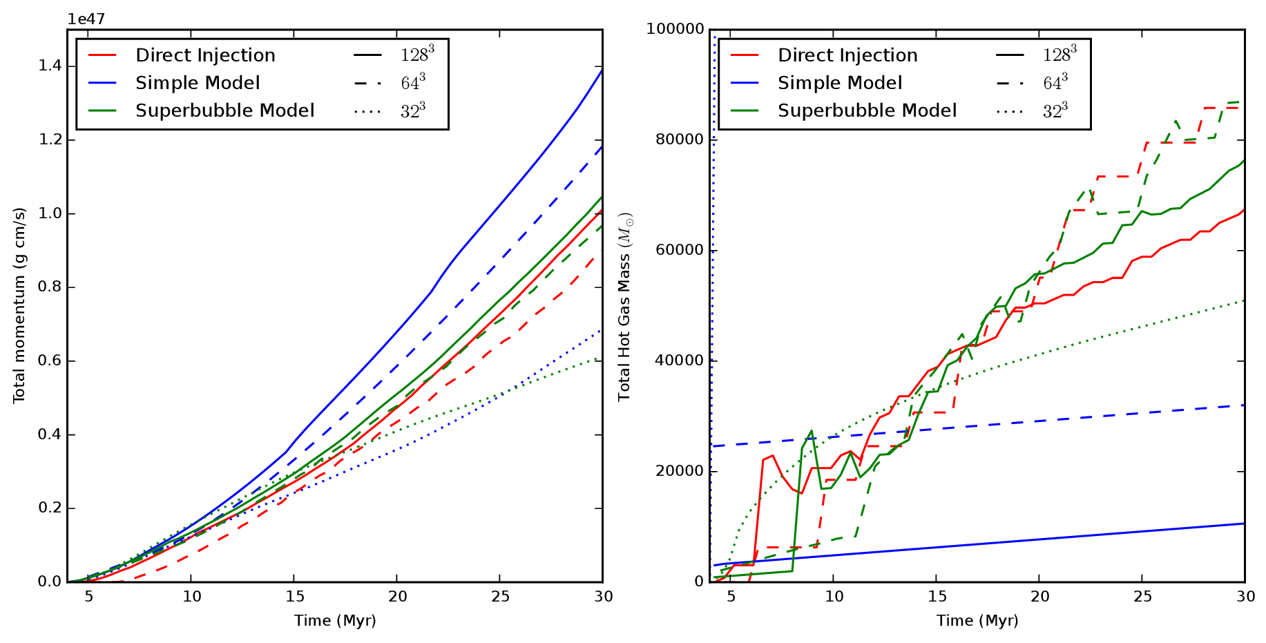
Figure 2: Feedback effects as a function of resolution. The above figure shows on the left the total radial momentum imparted to the medium, and on the right the total amount of mass heated to above $10^{5}\;\mathrm{K}$. The red curves are the direct injection results, the blue corresponds to the simple feedback, while the green shows the results of the superbubble model. Solid lines show the values from simulations run with resolutions of $128^{3}$ particles, dashed for $64^{3}$, and dotted for $32^{3}$. Note that for the $32^{3}$ run, the simple model produces $\sim 2\times 10^{5}\;M_{\odot}$ of hot gas.

2.3 Multiphase Fluid Elements

When feedback energy is deposited in a low-resolution simulation, or is deposited as a luminosity, the temperature and density are certain to be under- and over-estimated respectively. This problem leads to the well-known overcooling problem that has typically been addressed by disabling cooling for some amount of time for feedback-heated gas (e.g. Stinson et al. (2006), Springel & Hernquist (2003), or by stochastic feedback heating, where the temperature change of a fluid element heated by feedback is fixed to a constant value (e.g. Dalla Vecchia & Schaye (2012). We employ a third option: storing feedback energy in a second phase that is in pressure equilibrium with the rest of the fluid inside an element.

Fluid elements (gas cells or particles) enter the multi-phase state if they are given energy from feedback, and if their temperature is below $10^{5}\;\mathrm{K}$ (the ‘hot’ threshold). Multiphase elements have two values for their mass and energy, related to their total mass $m$ and energy $E$ by:

$$m=m_{\rm hot}+m_{\rm cold}\\ E=u_{\rm hot}m_{\rm hot}+u_{\rm cold}m_{\rm cold}$$ (7)

Assuming pressure equilibrium, both phases will have the same pressure $P$, and their densities are found using this and the total density $\rho$:

$$\frac{P}{\rho}=\frac{(\gamma-1)E}{m}$$ (8)

$$\rho_{\rm cold}=\frac{P}{(\gamma-1)u_{\rm cold}}\\ \rho_{\rm hot}=\frac{P}{(\gamma-1)u_{\rm hot}}$$ (9)

Both the cold and hot phases are allowed to radiatively cool using their separate temperatures and densities. When $PdV$ work is done to a multiphase particle, it is shared between the two phases weighted by their respective fraction of the total energy E,

$$\dot{u}_{\rm PdV,cold}=m\ \dot{u}_{\rm PdV}\frac{u_{\rm cold}}{E}\\$$ (10)

$$\dot{u}_{\rm PdV,hot}=m\ \dot{u}_{\rm PdV}\frac{u_{\rm hot}}{E}.$$ (11)

In the absence of heating and cooling, this allows each phase to correctly maintain constant entropy as the densities change.

Mass flux between the hot and cold phase is calculated in a continuous manner consistent with the prior evaporation scheme. Each timestep, a multi-phase element evaporates a fraction of its cold phase into the hot phase,

$$\frac{{\rm d}M_{b}}{{\rm d}t}=\frac{16\pi\mu}{25k_{B}}\kappa_{0}(T_{\rm hot}^{5/2})\ h.$$ (12)

Once an element has evaporated all of its mass into the hot phase, or if the hot phase cools below $10^{5}\;\mathrm{K}$, it is returned to the single-phase state.

2.4 SPH Implementation

We implemented this method in the SPH code GASOLINE (Wadsley, Stadel & Quinn, 2004) with updates described in Shen, Wadsley & Stinson (2010). These include a sub-grid model for turbulent mixing of metals and energy. The heating and cooling include photoelectric heating of dust grains, UV heating and ionization and cooling due to hydrogen, helium and metals.

The SPH hydrodynamic treatment has had some further, key updates. We currently use a standard SPH density estimator but a geometric density average in the SPH force expression: $(P_{i}+P_{j})/(\rho_{i}\,\rho_{j})$ in place of $P_{i}/\rho_{i}^{2}+P_{j}/\rho_{j}^{2}$ where $P_{i}$ and $\rho_{i}$ are particle pressures and densities respectively. This force expression alleviates numerical surface tension associated with density discontinuities, which is important for correct Kelvin-Hemholtz instabilities and ablation of cold blobs (as in the Agertz et al 2010 ’blob’ test). A similar force expression was first proposed by Ritchie & Thomas (2001). Geometric density averaged force expressions are now employed in all modern SPH codes (e.g. Hopkins (2013), Saitoh2013, Kawata2013, Hu2014 and Read2010). As stated in Read2010 and Saitoh2013, a key requirement for correct results with the modified force expression is a consistent energy equation that conserves entropy (which we employ). This is important to correctly model strong shocks, such as Sedov blasts. The extreme temperature jumps at strong shocks also require the time-step limiter of Saitoh & Makino (2009). The modern SPH code papers listed above all employ these updates and demonstrate accurate solutions for strong shocks (e.g. Sedov blasts) and shear flows (e.g. Kelvin Helmholz instabilities and the destruction of cold blobs).

For the tests shown here we used the Wendland $C_{2}$ kernel detailed in Dehnen & Aly (2012) with 64 neigbours where the SPH smoothing distance is defined so that the kernel weight drops to zero at $2\,h$.

Sharp density contrasts, as seen in highly resolved superbubbles, can require additional checks on the neighbour finding component of the SPH method. For example, hot particles can inadvertently become hydrodynamically decoupled from cold ones for a fixed number of neighbours. A full set of cold neighbours can sit at the edge of the kernel, where their contribution is negligible. The hot particle can thus have a full set of neighbours but feel minimal forces. We increase the number of neighbours until at least $18$ neighbours are within $1.41\,h$.

With respect to heating and cooling, for this work we used the Ritchie & Thomas (2001) density when calculating cooling rates to sharpen the density contrast between hot and cold gas. This is particularly useful at lower resolution when the hot bubble is resolved with a small number of particles. This improves the ability of low resolution runs to give similar energy loss rates to high resolution versions.

Feedback can increase gas particle masses substantially in the rare event that a gas particle spends a lot of time within star clusters without forming a star itself. This can degrade the accuracy of the SPH method. We avoid this problem by splitting particles that exceed $4/3$ their initial mass into two equal mass particles with the same properties. This affects a very small fraction of the particles.

These modifications, along with detailed testing, will be discussed in a forthcoming paper on GASOLINE2. For reference, the quality of our results on the tests discussed here is similar to the results presented for other modern modified SPH codes (e.g. Hopkins, 2013).

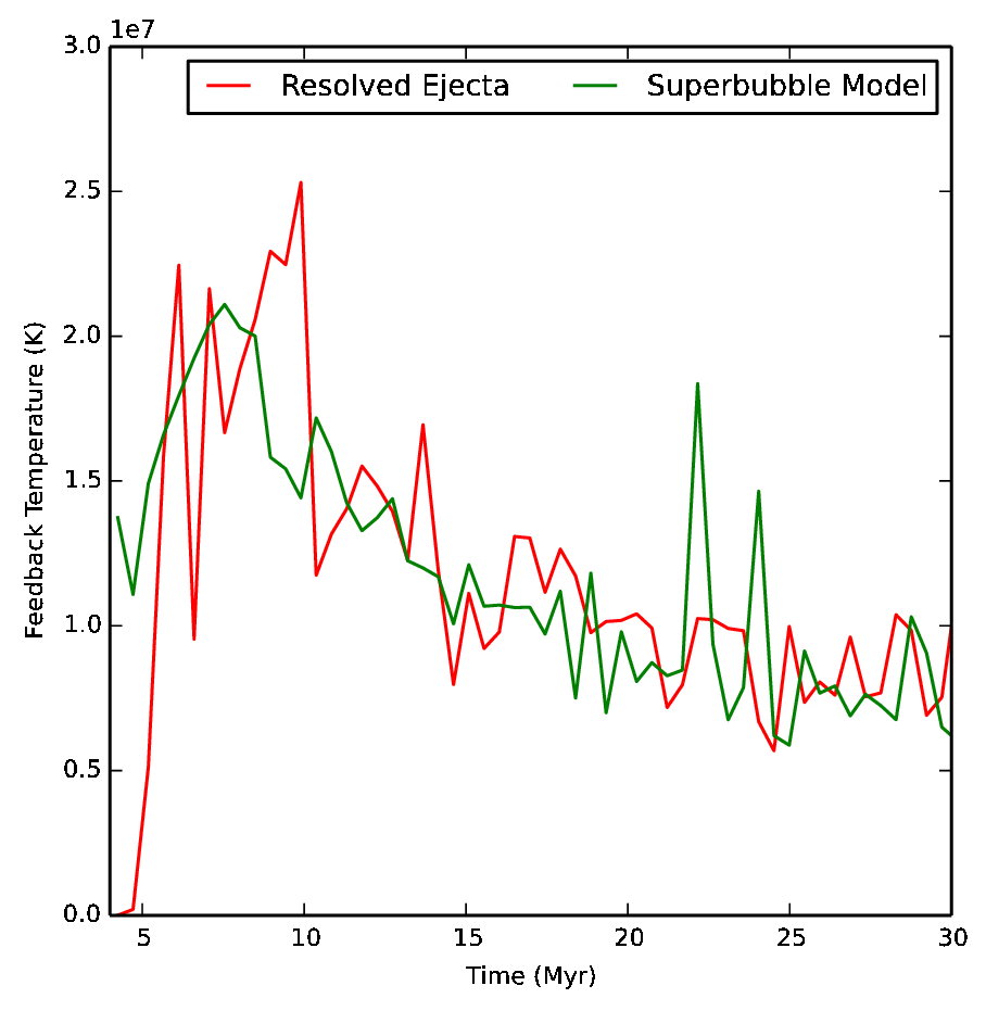
Figure 3: Peak temperature of feedback-heated gas inside the isolated star cluster’s hot bubble. Evaporation quickly enters the self-regulating regime, and the temperature is roughly constant for the last $15\;\mathrm{Myr}$ of feedback.

3 Simulations

3.1 High-Resolution Star Cluster Test

We began by exploring models of a single, isolated superbubbles at high resolution. For these tests, we employed three physical models. The Direct injection approach models as much physics as possible from first principles. Feedback mass and energy is modelled via a stream of new gas particles created from the star cluster. This approach only works when the gas resolution elements are much smaller than the star cluster mass. The only component of this model that is sub-grid is evaporation as this occurs on extremely small length scales. Superbubble Feedback refers to our new model. The key addition over the direct approach is the sub-grid multiphase treatment. Feedback energy and mass is injected into existing particles which may split.

We also include a Simple Feedback Model modeled after that proposed by Agertz et al. (2013). This model is a stand-in for models typically used to date and does not include conduction or evaporation. Feedback mass and energy is given to the nearest gas particle to the star cluster. This simple model incorporates a two-component energy treatment with radiative cooling disabled for feedback energy. Feedback energy is steadily converted into the regular, cooling form with an e-folding time of $5\;\mathrm{Myr}$.

3.1.1 Basic Superbubble

We placed a star cluster with mass $3\times 10^{4}\;\mathrm{M_{\odot}}$ in an uniform periodic box $2\times 2\times 2\;\mathrm{kpc}$ in size, containing $10^{3}\;\mathrm{K}$ gas with solar metallicity at a density of $1\;\mathrm{cm^{-3}}$. This gives a gas particle mass of $760\;M_{\odot}$, $6080\;M_{\odot}$, and $48640\;M_{\odot}$ for resolutions of $128^{3}$, $64^{3}$, and $32^{3}$ respectively. These tests do not include photoheating.

Figure 1 shows the column density projection for the three different feedback models in an isotropic medium. injection model. The hot interior of the bubble produced using the simple feedback model contains less mass at $128^{3}$ than the direct injection model and is subsequently too poorly resolved for the instabilities formed in the accelerated shell (Vishniac, 1983) to mix the bubble and shell through turbulence and diffusion.

As figure 2 shows, the superbubble feedback model performs much better than the simple model in reproducing the hot mass production rate from the high-resolution direct injection model, and lacks the extreme resolution sensitivity that the simple model exhibits for the amount of gas heated. The simple model only heats $\sim 4$ gas particles. For the $128^{3}$ and $64^{3}$ resolutions, this gives too little hot mass. For $32^{3}$ (extremely poor resolution, in fact with gas particles more massive than the entire cluster), this produces more than twice too much hot mass (more than $2\times 10^{5}\;M_{\odot}$). Meanwhile the simulation with the superbubble feedback model only underestimates the hot mass by roughly a third of the target $128^{3}$ direct injection simulation when used at a resolution $32^{3}$. The decreased momentum in the lower-resolution runs is likely due to particles staying longer in the multiphase state. More massive particles take longer to fully evaporate, and thus some mass that would be part of a pressure-driven cold shell at higher resolution is tied up in the cold part of multiphase particles.

Figure 3 shows that the actual peak temperature of the feedback-heated bubble in the isolated star cluster run is roughly $1\times 10^{7}\mathrm{K}$.

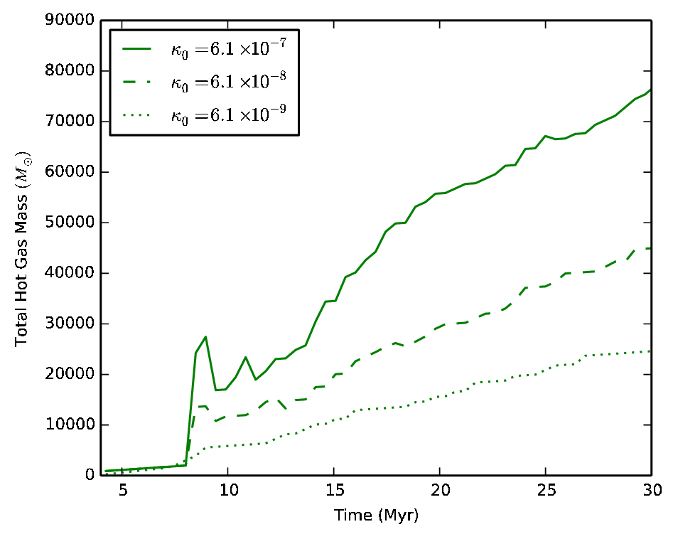
Figure 4: Hot mass production as a function of the conduction coefficient $\kappa_{0}$. As this figure shows, reducing $\kappa_{0}$ by a factor of 100 reduces the amount of hot mass generated through conduction by only a factor of $\sim 2$. All $\kappa_{0}$ values have units of $\mathrm{erg\;s^{-1}K^{-7/2}cm^{-1}}$.

3.1.2 Suppressed conduction

We also ran a set of simulations with the value of $\kappa_{0}$ used in the model reduced by a factor of 10 and a factor of 100. Since there is some uncertainty as to this coefficient in a magnetized ISM, we use this test to show that the self-regulating effect of conduction is insensitive to variation in $\kappa_{0}$.

Figure 4 shows the hot mass generated in simulations with 3 different values of $\kappa_{0}$. The dashed curve shows a reasonable lower limit for $\kappa_{0}$ (Cowie & McKee, 1977), while the dotted curve shows a much more extreme conduction reduction than is expected in nature. Both curves illustrate the insensitivity of the method to reductions in the conduction rate. Even reducing $\kappa_{0}$ by 100 only results in a reduction of the hot mass inside the bubble to just around a third.

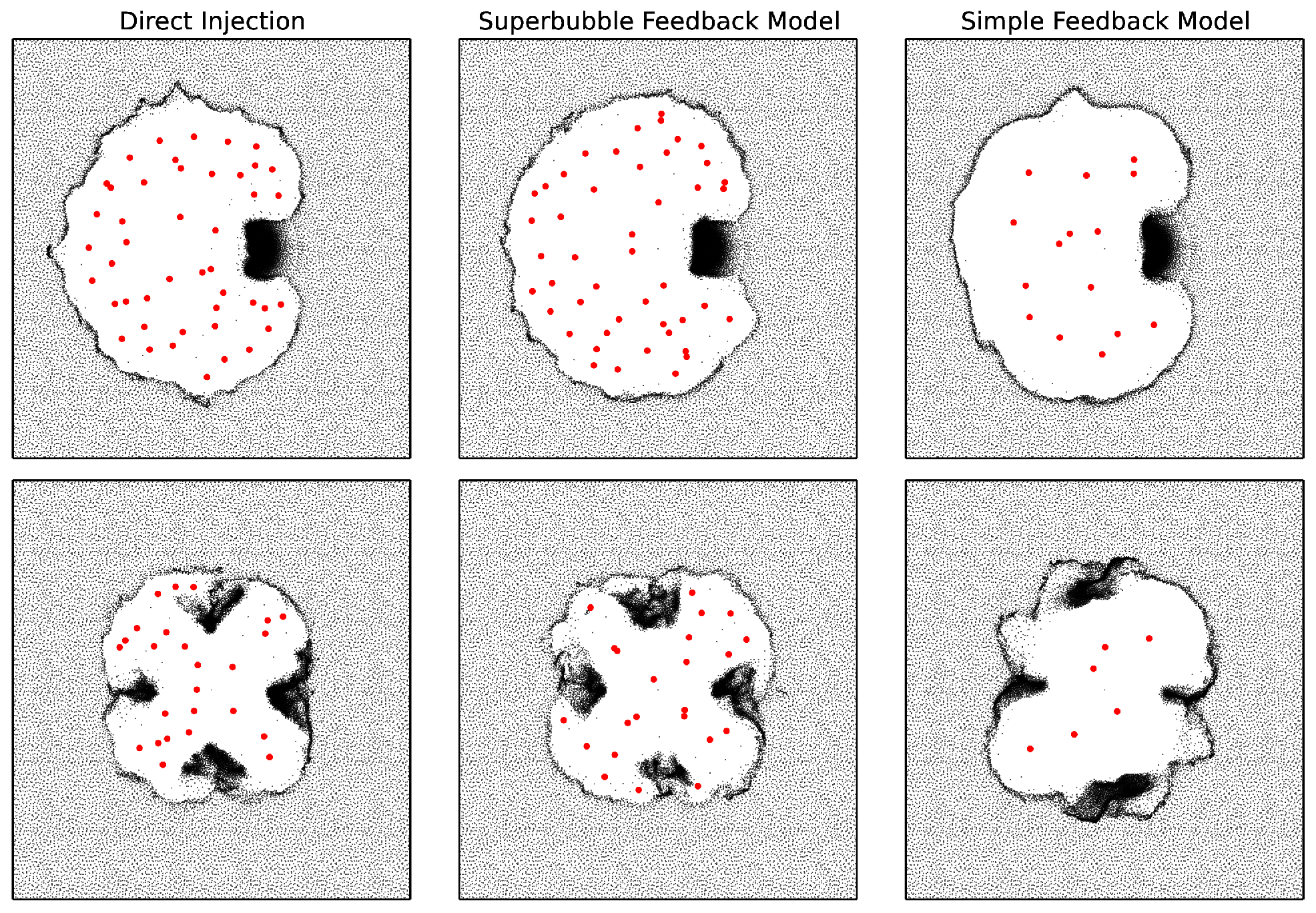
Figure 5: 3 kpc wide slices from the same three methods shown in figure 1, also at 50 Myr, but applied to a star cluster in an inhomogeneous medium. Particles whose smoothing length intersects z=0 kpc are shown. Particles above $10^{5}$ K are shown in red. The upper row shows simulations with a single clump, while the bottom row shows simulations with 6 clumps.

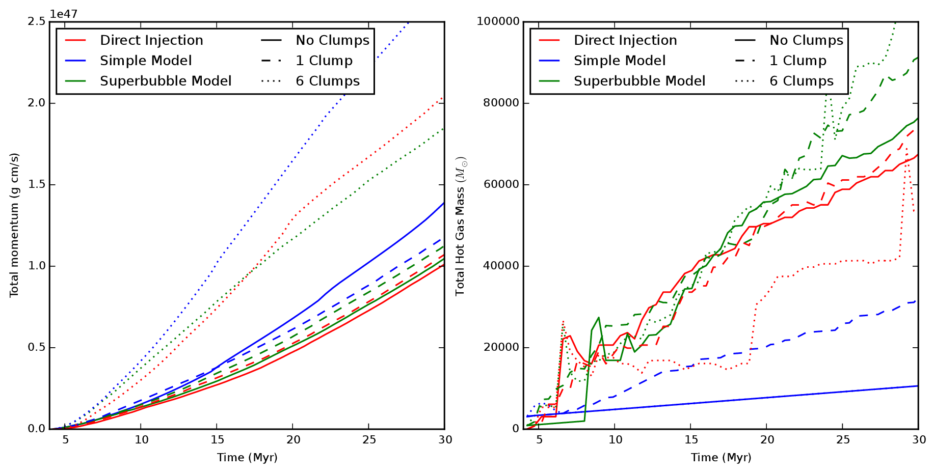
Figure 6: Feedback effects as a function of ISM homogeneity. The above figure shows on the left the total radial momentum imparted to the medium, and on the right the total amount of mass heated to above $10^{5}\;\mathrm{K}$. The red curves are the direct injection results, the blue corresponds to the simple feedback, while the green shows the results of the superbubble model. Solid curves show the results for a homogeneous ISM, dashed for a single dense clump, and dotted for 6 dense clumps.

3.1.3 Clumpy Medium

As the real ISM is highly inhomogeneous (and as Silich1996 showed, cold clumps can also be a source of evaporated cold material) , we ran two additional simulations with cold, dense clumps with $100\;\mathrm{cm^{-3}}$ density and $10\;\mathrm{K}$ gas in an ambient medium of $0.5\;\mathrm{cm^{-3}}$ at $1000\>\mathrm{K}$. This gives roughly the same amount of mass enclosed within the hot bubble at $30\>\mathrm{Myr}$. The first contains a single spherical clump with a radius of $0.2\;\mathrm{kpc}$. The second contains the same amount of cold mass spread over 6 clumps arranged at the center of each face of a cube $0.2\;\mathrm{kpc}$ surrounding the star. We use this idealized clumpy medium to test the sensitivity of the model to small scale structure that may be unresolved in lower resolution simulations. Figure 5 shows a slice showing SPH particles at $50\;\mathrm{Myr}$ for the two clumpy cases.

Figure 6 shows that the superbubble model is also capable of handling feedback into a clumpy medium. With more than an order of magnitude difference in the total hot mass compared to the simple model, along with less sensitivity to environment or resolution, the superbubble model is better suited for probing galactic outflows in simulations.

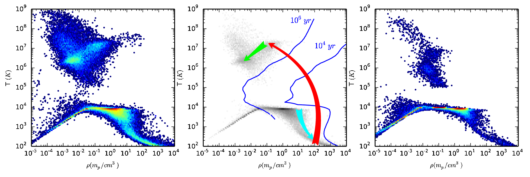
Figure 7: Phase diagrams for the Milky Way (left) and dwarf (right) simulations at $200\;\mathrm{Myr}$. The central panel shows a typical path for gas ejected from the Milky Way. First gas cools radiatively (cyan path) to high density, where it becomes multiphase as its hot component is heated to $\sim 10^{7}\;\mathrm{K}$ by feedback (red path) from nearby stars formed from its neighbouring high density gas. The hot phase cools primarily through adiabatic expansion (green path). This process is often repeated one or more times, with gas that is entirely hot phase being ejected from the disc. Cooling times of $10^{4}\;\mathrm{yr}$ and $10^{6}\;\mathrm{yr}$ are shown in blue. The majority of the hot gas in the upper left quadrant of the phase diagram has cooling times $>10^{8}\;\mathrm{yr}$. The cooling curve for $10^{8}\;\mathrm{yr}$ passes through the green curve. Note that particles in the multiphase state show the temperature and density for each state as separate points. The mean properties of multiphase particles would place them in regions with short cooling times.

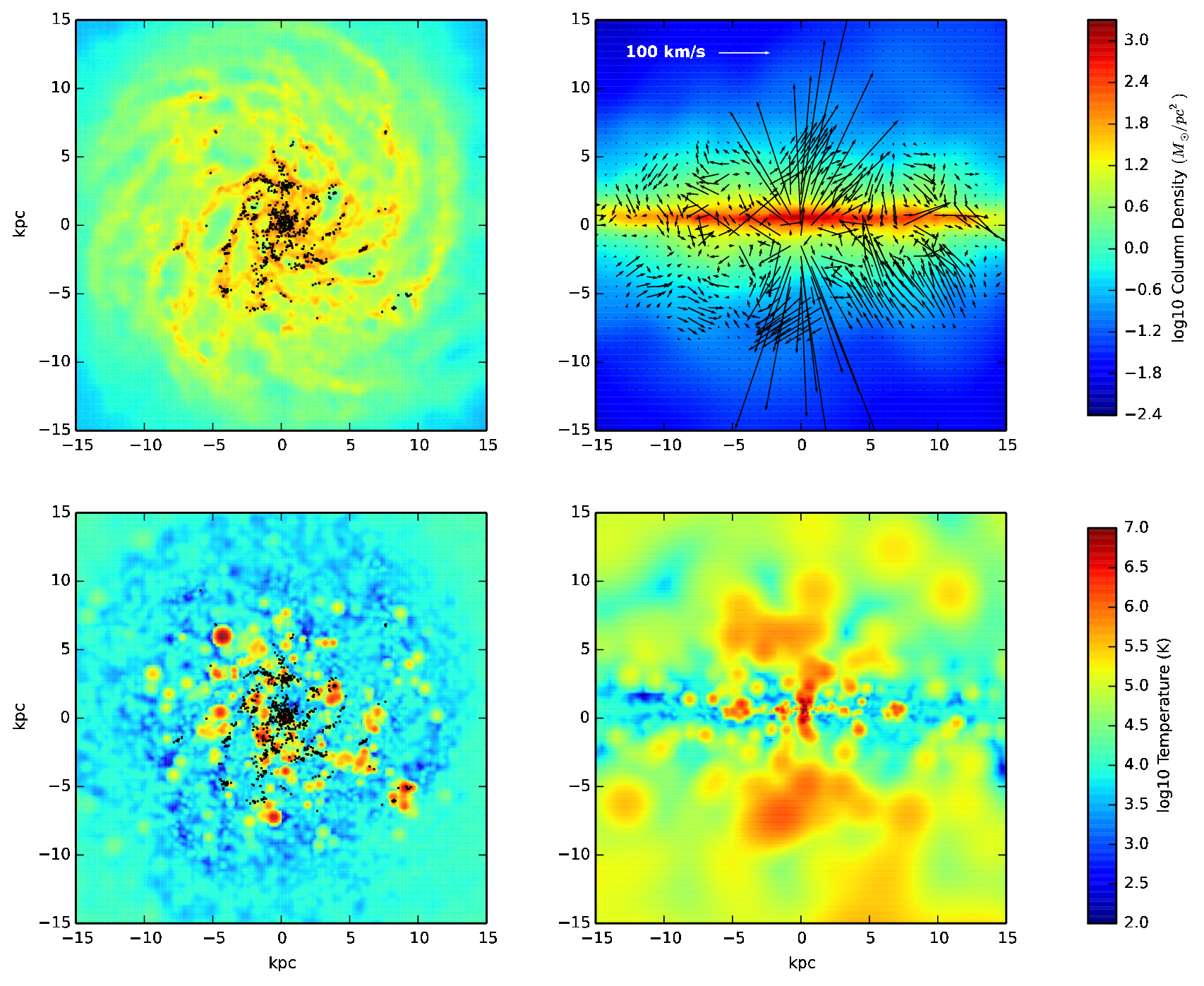
Figure 8: Column Density (upper row) and temperature for the Milky Way simulation at $300\;\mathrm{Myr}$. The vectors show the in-plane velocity. Temperatures shown are averages between the two phases for multiphase particles. Black points in the face-on images show stars formed within the last $20\;\mathrm{Myr}$. Note that gas is both leaving the disc near the galactic core, and returning in some places near the edge.

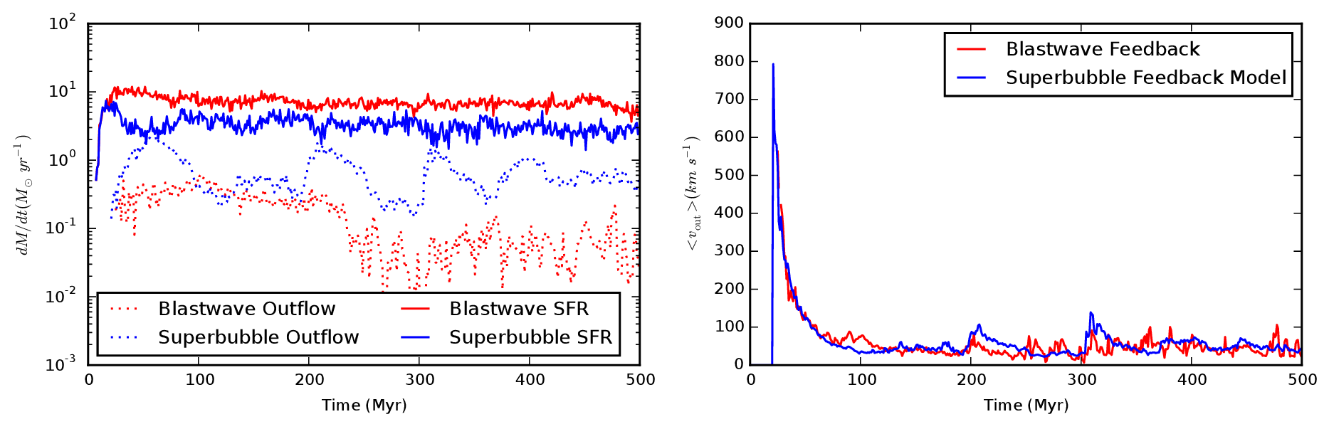
Figure 9: Outflow evolution for the Milky Way-like simulation. The left hand plot shows the star formation rate and the outflow rate The right hand plot shows the average outflow velocity.

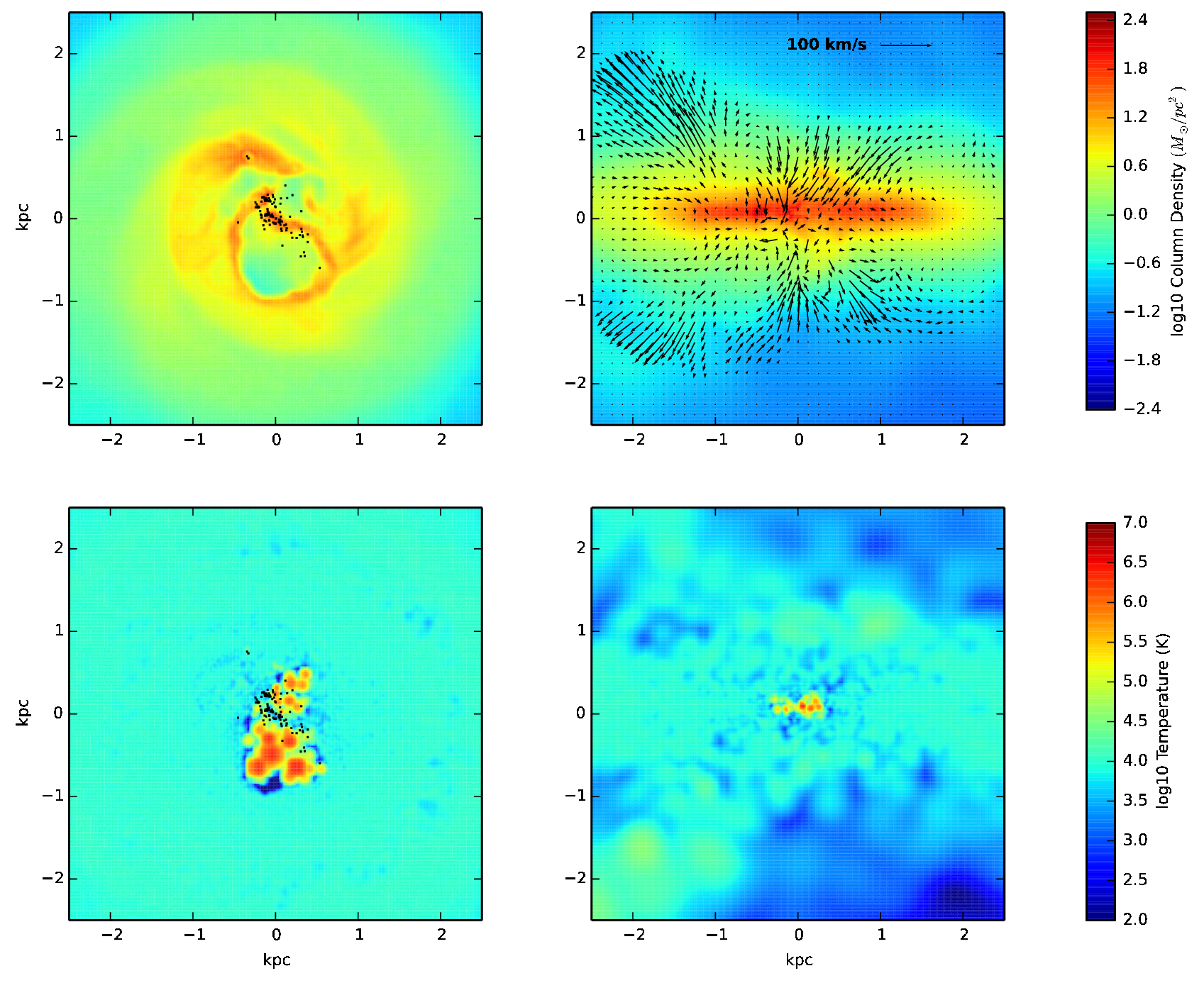
Figure 10: Column Density (upper row) and temperature for the dwarf simulation at $300\;\mathrm{Myr}$. The vectors in show the in-plane velocity. Temperatures shown are once again averages between the two phases for multiphase particles. Note the much more ‘puffed up’ appearance compared to the Milky Way, due to the more mass-loaded winds

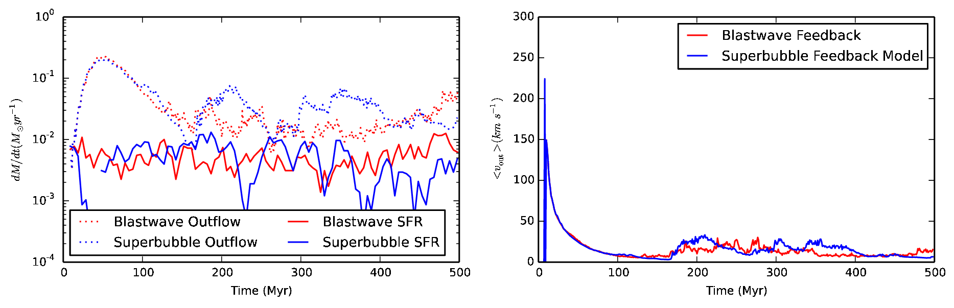
Figure 11: Outflow evolution for the dwarf galaxy. Note that the vertical ranges are different than in figure 9

3.2 Galaxy Simulations

3.2.1 Initial Conditions and Parameters

We used the isolated disc galaxy initial condition from the AGORA comparison project (Kim et al., 2013). These initial conditions were generated using the equilibrium disc generating code of Springel, Di Matteo & Hernquist (2005). This galaxy is similar to a MW-type spiral galaxy at $z=0$. For our dwarf simulation, we scaled the masses down by a factor of 100, and the length scales by a factor of $100^{1/3}$, preserving the physical densities in the initial conditions and lowering the surface density. The dwarf is thus similar to a low surface density local dwarf spiral. These initial conditions were intended to be similar to the $G10$ and $G12$ initial conditions used in Dalla Vecchia & Schaye (2012). The properties of these initial conditions are shown in table 1. Both simulations have 312500 total particles and 100000 gas particles, so that the mass resolution is substantially higher in the dwarf. The initial gas metallicity is solar in both cases.

We used the standard GASOLINE star-formation recipe, based on the algorithm proposed by Katz (1992) and detailed further in Stinson et al. (2006). We use a density threshold for star formation $n_{SF}$ shown in table 1 along with a temperature threshold of $T<10^{4}\;\mathrm{K}$. Thus, for a given eligible gas particle, the probability of forming a star each timestep $P_{SF}=1-\exp{-0.05\ \Delta t\over t_{\rm ff}}$, depends only on the free-fall time $t_{\rm ff}$. This corresponds to the effective star formation density rate of $\dot{\rho}_{*}=0.05\ \frac{\rho_{gas}}{t_{\rm ff}}$. We also include UV heating for $z=0$ (as in Shen, Wadsley & Stinson, 2010) and a pressure floor that ensures gas does not collapse beyond the resolvable Jeans length (Machacek, Bryan & Abel, 2001).

We also simulated these initial conditions using the established ‘blastwave’ feedback model from (Stinson et al., 2006), which has been a standard feedback model for galaxy simulations in numerous previous studies.

Simulation	$M_{tot}\mathrm{(M_{\odot})}$	$M_{gas}\mathrm{(M_{\odot})}$	$\epsilon\mathrm{(pc)}$	$n_{SF}\mathrm{cm^{-3}}$
Milky Way	$1.3\times 10^{12}$	$8.6\times 10^{9}$	20	$>10$
Dwarf	$1.3\times 10^{10}$	$8.6\times 10^{7}$	4.3	$>50$

Table 1: Disc galaxy initial conditions. $\epsilon$ is the gravitational softening and $n_{SF}$ is the star formation threshold.

3.2.2 ISM properties and Star Formation Rates

Figure 7 shows phase diagrams from both Milky Way and dwarf galaxies. Figure 8 shows column density and temperature for the Milky Way, and figure 9 shows star formation rates and outflow properties. Figures 10 and 11 show the same for the dwarf galaxy. The Kennicutt-Schmidt relation for both galaxies is shown in figure 12. The star formation and outflow properties are discussed in section 3.2.3. Finally, we show some properties of the multiphase particles in figure 13.

Figure 7 shows that phase diagrams for galaxies using superbubble feedback strongly distinguish between pre- and post-feedback gas. Above $\sim 10^{5}\;\mathrm{K}$, we see (especially in the Milky Way), a hot medium of including halo gas and low density gas inside superbubbles within the galaxy disc (see the temperature slices in figures 8 and 10 for images of the gas temperature in these bubbles). The bulk of the gas lies at a roughly $10^{4}\;\mathrm{K}$ equilibrium between cooling and photoheating from the UV background. A cold medium of both dense shells surrounding superbubbles and cooling clouds (soon to form stars) also forms in both the Milky Way and (to a lesser extent) the dwarf. The central panel shows a schematic of how gas migrates between these regions. Radiative cooling (blue arrow), bring gas to high densities. Feedback creates a second hot phase in nearby gas particles. The cold component is relatively unaffected though it can compress due to the increased pressure (staying near the tip of the blue arrow). The hot and cold phases of multiphase particles are plotted separately. The hot component immediately moves to low density and high temperatures, $\mathrel{\hbox to0.0pt{\lower 3.0pt\hbox{$\mathchar 536\relax$}\hss}\raise 2.0pt\hbox{$\mathchar 318\relax$}}10^{7}$ K (the red arrow). If the particle continues to receive feedback, evaporation rapidly consumes its cold part and the particle can flow out to the halo and remain buoyant and slow cooling. It evolves adiabatically as it does so (green arrow).

This panel is telling in that it shows that no gas is found within the ‘forbidden’ region of short cooling times of $\mathrel{\hbox to0.0pt{\lower 3.0pt\hbox{$\mathchar 536\relax$}\hss}\raise 2.0pt\hbox{$\mathchar 316\relax$}}10^{4}\;\mathrm{yr}$. Cooling-shutoff methods often produce large quantities of this gas in a high temperature, high density state. If we were to simply take the average temperature and density of the multiphase particles, they would almost entirely lie within this region, on the line connecting the cold and hot phases (which, of course, is exactly the impetus for using multiphase particles, since a particle with the average properties would cool away all of its feedback energy much too rapidly).

The roughly fixed amount of gas heated in the superbubble simulations shown previously gives a roughly constant feedback-heated gas temperature of $\sim 2\times 10^{7}\;\mathrm{K}$. Figure 3 shows that the actual peak temperature of the feedback-heated bubble in the isolated star cluster run varies between slightly less than this, to $\sim 1\times 10^{7}\mathrm{K}$, due to some cooling in the hot bubble. This suggests that the model should behave similarly to the stochastic thermal feedback model presented in Dalla Vecchia & Schaye (2012).

As the multiphase fluid particles exist to bridge the gap between when the hot interior of a superbubble contains too little mass to be resolved and the later stage when resolved physics can take over, we should find that particles stay in this phase for only a fraction of the lifetime of a superbubble. From Mac Low & McCray (1988), the cooling time for superbubbles is on the order of a few $10\;\mathrm{Myr}$, with a weak dependence on feedback luminosity and the surrounding ISM density and metallicity.

We should expect that on average, multiphase particles convert back to single phase in less than this time, a few $\mathrm{Myr}$. In addition to their lifetimes, we should expect multiphase particles to cluster in the discs of our galaxy simulations (since they are spatially correlated with the stars that are heating them), and that hot winds leaving the galaxy are composed of fully-resolved, hot gas. These winds are released when superbubbles grow large enough to break out of the denser disc ISM, and thus should be well within the resolved phase for these simulations.

Figure 13 shows the that all particles stay in the multiphase state as well as the maximum height reached by multiphase particles. The top figure shows that the vast majority of particles in either the dwarf or the Milky Way convert back to single phase within $10\;\mathrm{Myr}$. The mean multiphase lifetime for the Milky Way was $6.6\;\mathrm{Myr}$, and $2.7\;\mathrm{Myr}$ for the dwarf, well within the range we should expect. The reason for the shorter multiphase lifetimes in the dwarf galaxy is simply the better mass resolution: the hot bubble interior becomes resolved earlier in the dwarf than in the Milky Way. Fewer than 0.5 per cent of multiphase particles ever stay in the multiphase state for more than $50\;\mathrm{Myr}$ in both the Milky Way and the dwarf. The bottom figure shows, again as we should expect, that most multiphase particles convert back to single phase before they reach 1 scale height. The mean maximum height for multiphase particles was roughly $1/2$ a scale height for both simulations, $0.51\;\mathrm{kpc}$ and $0.13\;\mathrm{kpc}$ for the Milky Way and dwarf respectively. Neither simulation had any multiphase particles reaching heights of more than $10\;\mathrm{kpc}$ before converting back to single phase. This shows that multiphase particles are essentially embedded within the thin disc of the ISM: all of the mass outflowing is fully-resolved hot gas, and its behaviour is fully governed by standard hydrodynamics. The winds driven from both galaxies are ejected through nothing more than simple buoyancy.

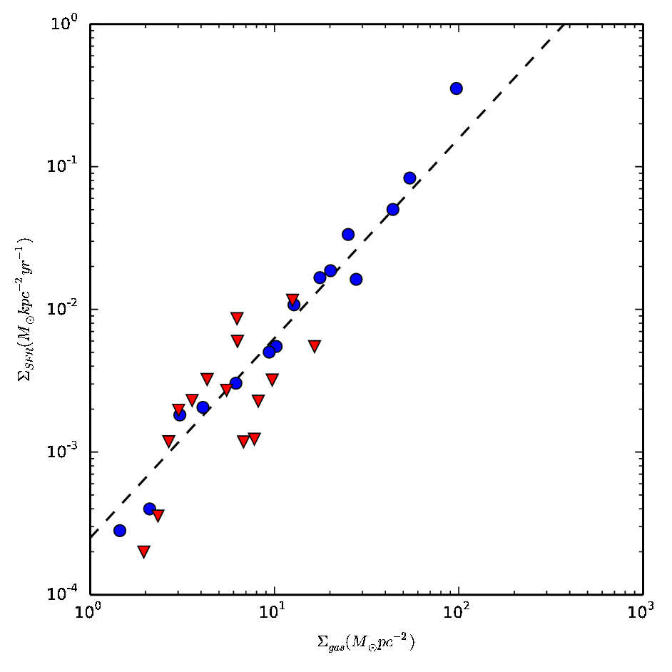
Figure 12: Kennicutt-Schmidt law in the Milky Way-like (blue points) and dwarf (red triangles) galaxies at $500\;\mathrm{Myr}$. Surface densities were calculated in radial annuli. The dashed line shows the Kennicutt-Schmidt Law. The superbubble model is easily able to regulate star formation rates to within this range.

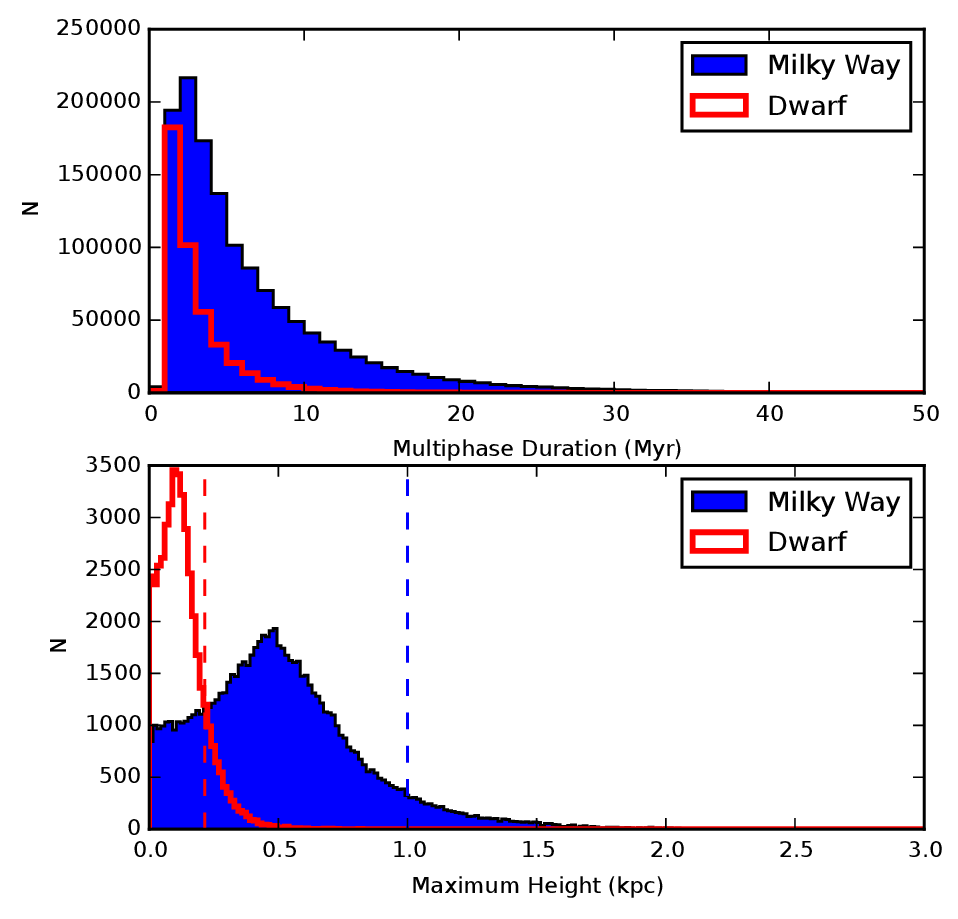
Figure 13: Properties of multiphase particles in the galaxy simulations. The top figure shows duration of multiphase state for particles in both galaxy simulations. Particles that are in the multiphase state more than once (convert back to single phase, cool, and then receive feedback again) have each time they are multiphase counted separately. The bottom figure shows maximum heights reached by particles in the multiphase state. For each particle that is ever in the multiphase state, the maximum height it reaches while still multiphase is shown above for both galaxy simulations. Dashed lines show scale heights at $10^{4}\;\mathrm{K}$ for each of the two simulations.

3.2.3 Galaxy Morphology and Outflows

In order to compare superbubble feedback to Dalla Vecchia & Schaye (2012), we selected similar galaxies to the ones shown in their paper and calculated the properties of their outflows using a similar method. We adopt their two primary metrics, mass outflow rate $\dot{M}$ and mean outflow velocity $<v_{\rm out}>$. These two metrics give us an idea as to both how much gas is ejected from the galaxies, and how long that gas will take to return to the disc from the halo (if it does return at all).

We calculated outflows from our galaxy simulations by selecting particles that are moving away from the galaxy between a planar region 5 scale heights (5kpc for the Milky Way, 1.13kpc for the dwarf) above and below the disc, and 0.5 scale heights thick. The outflow rate $\dot{M}$ is simply the total momentum of outflowing particles (particles returning on fountains are excluded) passing through this region divided by the thickness of the region. The average outflow velocity $<v_{\rm out}>$ is just the mean velocity of these same particles.

The superbubble feedback method, as shown in figure 12 (and the SFR shown in figures 9 and 11), also passes the most basic requirement for a useful feedback model: it is capable of regulating star formation to match observed global star formation efficiencies. This result is a typical outcome for effective feedback models with density-based star formation rates (e.g. Springel & Hernquist, 2003). Note that the simple star formation prescription used for these tests does not have a cut-off at lower surface densities. It is clear in figure 9 that the average SFR in the Milky Way is roughly twice as high in the simulation using blastwave feedback as compared to the simulation with superbubble feedback. It is also clear from this figure that outflows in the Milky Way simulation with superbubble feedback contain approximately ten times the mass of outflows driven by blastwave feedback.

4 Discussion

It is important to heat the right amount of gas through feedback. This is particularly important if one wishes to examine feedback-driven galactic winds. As figures 2 and 6 show, the simple cooling-shutoff feedback model produces quite different amounts of hot gas as a function of both resolution and ISM homogeneity. If one underestimates the amount of mass heated by feedback, the winds one drives will be hotter, but contain less mass. In other words, outflows will be faster but contain less mass. If one overestimates the amount of mass, outflows may carry a larger fraction of the galaxy’s gas mass, but will be less able to actually remove this gas from the galaxy, either permanently or for a long cycling timescale. Either error will have serious implications for predictions of the effects of outflows on both host galaxies and the intergalactic medium. We have constructed our model such that both the momentum and the amount of hot gas within a superbubble are resolution independent. This is confirmed in figure 2 over a range of mass resolutions from $\sim 95M_{\odot}$ to $5\times 10^{4}M_{\odot}$. Even in the extreme limit of a one particle superbubble, the results are qualitatively correct and vary less than a factor of 2 from the expected solution.

In fact, for any feedback model that omits thermal conduction or other mixing between the hot interior of a feedback bubble and the surrounding cold shell, the amount of hot mass produced will be set by the resolution of the simulation alone. In fact, figure 2 shows this quite clearly. For each resolution, the hot mass produced is roughly constant, simply a product of the simulation mass resolution and the number of particles feedback is shared with. Changing either of these will drastically change the amount of hot gas generated by feedback.

In general, the gas driven in outflows from these galaxies does not move fast enough to escape the galactic halos in either the dwarf and the Milky Way. This is reasonable for star formation rates well below the starburst regime. The majority of gas ejected from both simulations instead cycles between the halo and the disc. This helps moderate star formation in the disc. By $300\;\mathrm{Myr}$, only $\sim 1.0$ per cent, or roughly $8.4\times 10^{7}\;\mathrm{M_{\odot}}$, of the Milky Way gas has been lifted to above 5 scale heights while the dwarf cycles more than a third of its total gas mass, $3.3\times 10^{7}\;\mathrm{M_{\odot}}$ into a fountain above 5 scale heights. In both simulations, this cycling induces periodic bursts of star formation and disc outflows.

As figures 9 and 11 show, the superbubble method results in galaxies with stronger star formation regulation, and more mass-loaded outflows than the well-established blastwave model. For example, the simulation of the Milky Way analog, the star formation rate is lower by a roughly a factor of 2 compared to the blastwave (a point in favour of the superbubble model, since Scannapieco et al. (2012) showed that a cosmological simulation of the Milky Way using blastwave feedback in GASOLINE formed stars at roughly twice the rates observed by Guo et al. (2011)). We also see roughly an order of magnitude more gas ejected from the disc with the superbubble model, as we expect from the results of the single star cluster test, since the production of more hot mass should result in more mass-loaded winds. Interestingly, the mean outflow velocity shows only small differences between the superbubble and blastwave models. This means that even though the outflows driven by the blastwave contain less mass, they do not leave the galaxy any faster, and are no more likely to escape the galactic potential than winds produced in the superbubble simulations.

Our superbubble model is comparable to the model of Dalla Vecchia & Schaye (2012) with a $\Delta T\sim 10^{7}\;\mathrm{K}$, somewhat smaller than their fiducial value. Both heat of order $300\;\mathrm{M_{\odot}}$ per SNe. Dalla Vecchia & Schaye (2012) simply relied on a stochastic model to deposit enough energy only when a specified temperature can be reached. Their model suffers from overcooling at cosmological resolutions with densities $n_{H}>10\;\mathrm{cm^{-3}}$ as their stochastic model requires the heating of fractional gas particles to yield the temperatures they desire. At moderate resolution, some star forming regions thus experience no feedback and others get strong feedback. The multiphase mechanism can handle resolutions where the initial feedback-heated gas mass is less than a single resolution element, without relying on stochastic feedback.

The superbubble method has a number of distinct advantages over previous feedback methods (cooling shutoffs, constant-temperature stochastic feedback, hydrodynamic decoupling, etc.). The superbubble model introduces no additional free parameters, requiring only the total stellar feedback energy to be specified. The superbubble paradigm can incorporate multiple sources of mechanical luminosity, primarily stellar winds and supernovae, within a single framework. Unlike other methods, the amount of mass heated by feedback is physically motivated: it is the amount of mass evaporated into the hot bubble through thermal conduction. Radiative cooling is suppressed not by simply disabling it (which at best only approximates the long cooling times desired), but by injecting energy into a distinct low density, hot phase. This allows the model to handle high-resolution isolated galaxy simulations as well as lower-resolution cosmological ones.

Another distinct advantage of this method is that it is local. Feedback-heated gas needs no knowledge of its environment save the information it has already through hydrodynamic interactions with its neighbours. This allows the method to handle feedback from clustered star formation without any additional changes; gas particles need not know the total energy inside a feedback-heated superbubble, which can be difficult to determine in a bubble that is heated by multiple stars and contains many gas particles or cells. Clustered star formation is an important aspect of galactic evolution, and can amplify the effects of feedback by concentrating it on a single region (something done by hand in stochastic, constant temperature feedback models). As resolution in galaxy simulations has been steadily improving, well-resolved clustered star formation is beginning to become a reasonable goal and object of study. The superbubble model will allow feedback from these clusters to behave in a physically correct manner that is insensitive to resolution.

4.1 Summary

Stars preferentially form in clusters. Clustered stellar feedback generates superbubbles which are qualitatively different to isolated supernovae. Correctly evolving superbubbles requires the inclusion of thermal conduction. Thermal conduction, acting on very small length scales, evaporates cold material into hot feedback bubbles which must be captured via a sub-grid evaporation model such as the one presented here. At the typical resolutions achievable in galaxy simulations, a sub-grid multiphase treatment is required to accurately follow the evolution of the hot phase. Combining these elements results in a feedback model with several attractive features:

1. Separate hot and cold phases within an unresolved superbubble prevent overcooling without relying on ad-hoc cooling shutoffs

2. Feedback from multiple sources (e.g. star clusters) is combined correctly

3. Feedback gas doesn’t unphysically persist in phases with extremely short cooling times

4. Star formation is strongly regulated: at least as effectively as current models with the same feedback energy

5. The feedback can effectively drive outflows

6. Evaporation due to thermal conduction generates the correct amount of hot gas which subsequently determines galactic wind mass-loading

7. For well resolved bubbles, the model no longer relies on its multiphase component and naturally produces superbubbles that behave as predicted

8. The model is insensitive to resolution

References

- Agertz et al. (2013) Agertz O., Kravtsov A. V., Leitner S. N., Gnedin N. Y., 2013, ApJ, 770, 25
- Chabrier (2003) Chabrier G., 2003, PASP, 115, 763
- Chevalier (1974) Chevalier R. A., 1974, ApJ, 188, 501
- Cowie & McKee (1977) Cowie L. L., McKee C. F., 1977, ApJ, 211, 135
- Dalla Vecchia & Schaye (2012) Dalla Vecchia C., Schaye J., 2012, MNRAS, 426, 140
- Davé et al. (1998) Davé R., Hellsten U., Hernquist L., Katz N., Weinberg D. H., 1998, ApJ, 509, 661
- Dehnen & Aly (2012) Dehnen W., Aly H., 2012, MNRAS, 425, 1068
- Dubois & Teyssier (2008) Dubois Y., Teyssier R., 2008, A&A, 477, 79
- Durier & Dalla Vecchia (2012) Durier F., Dalla Vecchia C., 2012, MNRAS, 419, 465
- Gerritsen (1997) Gerritsen J. P. E., 1997, PhD thesis, , Groningen University, the Netherlands, (1997)
- Guo et al. (2011) Guo Q. et al., 2011, MNRAS, 413, 101
- Hopkins (2013) Hopkins P. F., 2013, MNRAS, 428, 2840
- Hopkins, Quataert & Murray (2012) Hopkins P. F., Quataert E., Murray N., 2012, MNRAS, 421, 3522
- Katz (1992) Katz N., 1992, ApJ, 391, 502
- Kim et al. (2013) Kim J.-h., Abel T., Agertz O., for the AGORA Collaboration, 2013, ArXiv e-prints
- Leitherer et al. (1999) Leitherer C. et al., 1999, ApJS, 123, 3
- Mac Low & McCray (1988) Mac Low M.-M., McCray R., 1988, ApJ, 324, 776
- Machacek, Bryan & Abel (2001) Machacek M. E., Bryan G. L., Abel T., 2001, ApJ, 548, 509
- Marri & White (2003) Marri S., White S. D. M., 2003, MNRAS, 345, 561
- McKee & Ostriker (1977) McKee C. F., Ostriker J. P., 1977, ApJ, 218, 148
- Mihos & Hernquist (1994) Mihos J. C., Hernquist L., 1994, ApJ, 425, L13
- Nath & Shchekinov (2013) Nath B. B., Shchekinov Y., 2013, ApJ, 777, L12
- Navarro & White (1993) Navarro J. F., White S. D. M., 1993, MNRAS, 265, 271
- Pontzen et al. (2013) Pontzen A., Roškar R., Stinson G. S., Woods R., Reed D. M., Coles J., Quinn T. R., 2013, pynbody: Astrophysics Simulation Analysis for Python. Astrophysics Source Code Library, ascl:1305.002
- Ritchie & Thomas (2001) Ritchie B. W., Thomas P. A., 2001, MNRAS, 323, 743
- Saitoh & Makino (2009) Saitoh T. R., Makino J., 2009, ApJ, 697, L99
- Scannapieco et al. (2006) Scannapieco C., Tissera P. B., White S. D. M., Springel V., 2006, MNRAS, 371, 1125
- Scannapieco et al. (2012) Scannapieco C. et al., 2012, MNRAS, 423, 1726
- Sharma et al. (2014) Sharma P., Roy A., Nath B. B., Shchekinov Y., 2014, ArXiv e-prints
- Shen, Wadsley & Stinson (2010) Shen S., Wadsley J., Stinson G., 2010, MNRAS, 407, 1581
- Songaila & Cowie (1996) Songaila A., Cowie L. L., 1996, AJ, 112, 335
- Springel, Di Matteo & Hernquist (2005) Springel V., Di Matteo T., Hernquist L., 2005, MNRAS, 361, 776
- Springel & Hernquist (2003) Springel V., Hernquist L., 2003, MNRAS, 339, 289
- Stinson et al. (2006) Stinson G., Seth A., Katz N., Wadsley J., Governato F., Quinn T., 2006, MNRAS, 373, 1074
- Thacker & Couchman (2000) Thacker R. J., Couchman H. M. P., 2000, ApJ, 545, 728
- Vishniac (1983) Vishniac E. T., 1983, ApJ, 274, 152
- Wadsley, Stadel & Quinn (2004) Wadsley J. W., Stadel J., Quinn T., 2004, New Astronomy, 9, 137
- Weaver et al. (1977) Weaver R., McCray R., Castor J., Shapiro P., Moore R., 1977, ApJ, 218, 377