We present an approach to statistical data modeling and exploratory data analysis called ‘LP Statistical Data Science.’ It aims to generalize and unify traditional and novel statistical measures, methods, and exploratory tools. This article outlines fundamental concepts along with real-data examples to illustrate how the ‘LP Statistical Algorithm’ can systematically tackle different varieties of data types, data patterns, and data structures under a coherent theoretical framework. A fundamental role is played by specially designed orthonormal basis of a random variable $X$ for linear (Hilbert space theory) representation of a general function of $X$, such as $\mathbb{E}[Y\mid X]$.

Keywords: LP-representation; Exploratory big data analysis; Custom constructed LP orthonormal score functions; LP-moments; LP-Comoment; LP skew density; LP Checkerboard copula density estimation; LP smoothing; Correspondence analysis; LPINFOR; Sparse contingency table; Nonlinear dependence modeling; LP goodness-of-fit statistic .

 

0 Goals

There has been explosive growth of statistical algorithms in recent times, due to greater availability of data with mixed types (discrete or continuous), patterns (simple linear to complex nonlinear) and structures (univariate to multivariate). Growth in statistical software technology contributed substantially to simplify the implementation workloads of these various methods. While execution of an algorithm getting easier by pushing the button, the theory and practice of statistical learning methods are becoming more complicated day by day with the availability of thousands of ‘isolated’ statistical ideas and softwares. We seek a more systematic and automatic approach to develop interpretable algorithms that permits easy way to establish relationship among various statistical methods (thus simplifies teaching and facilitate practice). An attempt is made in this paper to describe how this can be done via a new theory ‘LP Statistical Data Science’. Our theory provides unified representation of statistical methods based on few fundamental functions (defined for both discrete and continuous random variables): Quantile function, custom-constructed LP orthonormal score functions, LP Skew density function, LP copula density function and LP comparison density function. We apply these tools to solve broad range of statistical problems like goodness-of-fit, density estimation, correlation learning, conditional mean and quantile modeling, copula estimation, categorical data modeling, correspondence analysis etc., in a coherent manner. We hope LP statistical learning theory might give us the clue for designing ‘United Statistical Algorithm’. We outline core mathematical concepts of the LP approach to data analysis, design applicable algorithms and illustrate using concrete real data examples.

1 LP Score Function

Our approach to nonparametric modeling is based on the representation of a general function $h(X)$ in an orthonormal basis of functions of $X$ (more precisely, functions of $F^{\rm{mid}}(x;X)$, the mid-distribution function of $X$), denoted by $T_{j}(x;X)$, called LP Score functions. LP unit score functions are orthonormal on unit interval defined as $S_{j}(u;X)=T_{j}(Q(u;X);X)$, $0<u<1$, where $Q(u;X)$ is quantile function of $X$.

1.1 Definition and Construction

Define Mid-distribution function of a random variable $X$ as

$$F^{\rm{mid}}(x;X)\,=\,F(x;X)-.5p(x;X),\,\,p(x;X)\,=\,\Pr[X=x],\,\,F(x;X)\,=\,\Pr[X\leq x].$$ (1.1)

For a mid-distribution $F^{\rm{mid}}(x;X)$ with quantile function $Q(u;X),0<u<1$, we construct $T_{j}(x;X)$, $j=0,1,\ldots$ orthonormal LP score functions by Gram Schmidt orthonormalization of powers of $T_{1}(x;X)$. Define $T_{0}(x;X)=1$ and

$$T_{1}(x;X)\,=\,\dfrac{F^{\rm{mid}}(x;X)-.5}{\sigma(F^{\rm{mid}}(X;X))}.$$ (1.2)

Parzen (2004) showed that $\mathbb{E}[F^{\rm{mid}}(X;X)]=.5$ and $\operatorname{Var}[F^{\rm{mid}}(X;X)]=(1-\sum_{x}p^{3}(x;X))/12$. Note that for $X$ continuous we have $T_{1}(x;X)=\sqrt{12}(F(x;X)-.5)$. LP unit score functions $S_{j}(u;X)$ are orthonormal in $L^{2}(F)$, the Hilbert space of square integrable functions on $0<u<1$, with respect to the measure $F$ (either discrete or continuous). When X is continuous, we recover the Legendre polynomials

$$S_{j}(u;X)\,=\,\operatorname{Leg}_{j}(u),\,\,\,\,T_{j}(X;X)\,=\,\operatorname{Leg}_{j}\big{[}F(X;X)\big{]}.$$ (1.3)

Formulas of orthonormal shifted Legendre polynomials on $[0,1]$ are given in Appendix A1.

1.2 Sufficient Statistics Interpretation

Models that are nonlinear in $X$ can be constructed in many applications as linear models of the score vector $TX$ with components $T_{j}(X;X)$, which we interpret as “sufficient statistic” for $X$. This approach is implemented for time series analysis in our theory of LPTime (Mukhopadhyay and Parzen, 2013).

Figure 1: Shapes of LP-unit score functions for (a) poisson distribution (with $\lambda=2$), and (b) discrete uniform distribution (which generates discrete Legendre polynomials) based on $n=250$ simulated samples.

Figure 2: Shapes of first four orthonormal shifted Legendre polynomials on $[0,1]$.

1.3 Relations with Legendre polynomials

For $X$ continuous, LP unit score functions yield Legendre polynomials, as shown in Fig 2. For $X$ discrete-uniform or for a sample distribution with all distinct values, LP score functions take the form of discrete Legendre polynomials, shown in Fig 1(b). General piecewise constant shape of orthonormal LP unit score functions for $X$ discrete random variable is shown in Fig 1(a), based on $n=250$ simulated samples from poisson with $\lambda=2$. Note that sample distributions are always discrete.

2 LP Moments, LP Comoments

The L moments method of data analysis, introduced by Hosking (1990), was pioneered by Sillitto (1969) in the paper “Derivation of approximants to the inverse distribution of a continuous univariate population from the order statistics of a sample.” The goal is nonparametrically estimate distribution function $F(x;X)$ of variable $X$ in a way that is systematic (not ad hoc) and avoids high powers of $X$ (moments). Sillitto (1969) shows that continuous $X$ can be expressed as a polynomial of $F(X;X)$, the rank transform, or probability integral transform of $X$. We extend this concept to general $X$, discrete or continuous, by introducing the concept of LP moments and the multivariate generalization LP-comoments. We provide a compact representation and computationally efficient algorithm to compute the exact (unbiased version) sample estimates, which is known to be a challenging problem (Hosking and Wallis, 1997).

2.1 LP Moments, Representation of X

Define LP moments as $\operatorname{LP}(j;X)=\mathbb{E}[XT_{j}(X;X)]$. An equivalent representation using LP unit score functions (by expressing in quantile domain) is

$$\operatorname{LP}(j;X)=\int_{0}^{1}Q(u;X)S_{j}(u;X)\;\mathrm{d}u,$$ (2.1)

which leads to the following important representation theorem by Hilbert space theory that provides nonparametric identification of models for mixed $Q(u;X)$ by estimating its LP moments.

Theorem 1.

Quantile function $Q(u;X)$ for a random variable $X$ with finite variance can be expressed as an infinite linear combination of LP unit score functions with coefficients as LP-moments

$$Q(u;X)-\mathbb{E}(X)=\sum_{j>0}\operatorname{LP}(j;X)\,S_{j}(u;X),$$ (2.2)

From Theorem 1 we derive the the following LP representation result of $X$ as a function of $F(X;X)$; It is similar to a Karhunen-Loéve expansion leading to a sparse representation of $X$ in a custom built orthonormal basis.

Theorem 2.

A random variable $X$ (discrete or continuous) with finite variance admits the following decomposition with probability $1$

$$X-\mathbb{E}(X)=\sum_{j>0}\operatorname{LP}[j;X]\,T_{j}(X;X),$$ (2.3)

We call (2.3) the LP representation of $X$. Theorem 2 is a direct consequence of applying the following fundamental theorem to (2.2).

Lemma 2.1.

For a random variable $X$ with probability $1$, $Q(F(X;X);X)=X$.

A published proof of this known fact is difficult to find; we outline proof in Appendix A2. Theorem 2 leads to a very useful fact about variance of $X$ given in the following corollary.

Corollary 2.1.

Variance decomposition formula in terms of LP moments

$$\operatorname{Var}(X)=\sum_{j>0}\big{|}\operatorname{LP}(j;X)\big{|}^{2}$$

Remark 1 (Interpretation of LP shape statistic).

For a sample of $X$ continuous with distinct values one can derive the following representation of $\operatorname{LP}[1;{\widetilde{F}}]$ as a linear combination of order statistics

$$\operatorname{LP}[1;{\widetilde{F}}]\,=\,\dfrac{2\sqrt{3}}{n\sqrt{n^{2}-1}}\sum_{i=1}^{n}\,X_{(i)}\Big{(}i\,-\,\dfrac{1}{2}(n+1)\Big{)}.$$

Our $\operatorname{LP}(1;X)$ is a measure of scale that is related to the Downton’s estimator (Downton, 1966) and can be interpreted as a modified Gini mean difference coefficient (David, 1968). Measures of skewness and kurtosis are $\operatorname{LP}(2;X)$ and $\operatorname{LP}(3;X)$.

Table 2 in Appendix A3 reports numerical values of LP moments for some standard discrete and continuous distributions. For the Ripley data (described in the next section), the first four sample LP moments of $X=$ Age are $4.74,1.49,0.27,0.11$ and $\operatorname{Var}(X)=24.84$. For $Y=$ GAG level, the first four sample LP moments are $8.08,2.90,1.89,1.05$ and $\operatorname{Var}(Y)=80.87$. The nonparametric robust LP moments provide a quick understanding of the shape of the marginal distributions, as depicted in Fig 4.

An application of LP moment to test of normality is given by the following result. For $X\sim\mathcal{N}(\mu,\sigma^{2})$ we have

$$\operatorname{LP}(1;X)\,=\,\sigma\,\mathbb{E}[X\operatorname{Leg}_{1}(\Phi(X));X]\,=\,2\sqrt{3}\,\sigma\,\mathbb{E}[\phi(X);X]\,=\,\sqrt{3/\pi}\,\sigma.$$ (2.4)

This suggests that D’Agostino’s normality test (D’Agostino, 1971) can be computed as

$$\operatorname{Cor}(X,F(X))~{}=~{}\operatorname{LP}[1;X]/\sigma.$$ (2.5)

Define $X$ to be short tailed if $|\operatorname{LP}(1;\mathcal{Z}(X)]|^{2}>.95$, where $\mathcal{Z}(X)=(X-\mathbb{E}[X])/\sigma$.

2.2 LP Comoments, Dependence Analysis

To model dependence and joint distribution of $(X,Y)$, define LP comoments as the cross-covariance between higher-order orthonormal LP score functions $T_{j}(X;X)$ and $T_{k}(Y;Y)$,

$$\operatorname{LP}[j,k;X,Y]~{}=~{}\mathbb{E}[T_{j}(X;X)\,T_{k}(Y;Y)]~{}~{}~{}\mbox{for}~{}j,k>0.$$ (2.6)

From the LP-representation (2.3) of $X$ and $Y$ we obtain following expansion of covariance based on LP-comoments and LP-moments.

Theorem 3.

Covariance between $X$ and $Y$ admits the following decomposition

$$\operatorname{Cov}(X,Y)~{}=~{}\sum_{j,k>0}\operatorname{LP}(j;X)\operatorname{LP}(k;Y)\operatorname{LP}(j,k;X,Y)$$ (2.7)

Table 2 in Appendix A4 lists LP comoments of bivariate standard normal with correlation $\rho$ equal $0,.5,.9$.

2.3 Ripley GAG Urine Data, Fisher Hair and Eye Color Data

We will be using the following two interesting data sets to demonstrate how our LP algorithms answer scientific questions.

Example 1 (Ripley GAG Urine Data).

This data set was introduced by Ripley (2004). The study collected the concentration of a chemical GAG in the urine of $n=314$ children aged from zero to seventeen years. The aim of the study was to produce a chart to help paediatricians to assess if a child’s GAG concentration is ‘normal.’ In Section 7.4 we present our comprehensive analysis of this data set. Eq. (2.8) computes the empirical LP-comoment matrix of order $m=4$ between $X$ Age and $Y$ GAG level for the Ripley data:

$$\widehat{\operatorname{LP}}\big{[}X,Y\big{]}~{}=~{}\begin{bmatrix}-0.908^{*}&-0.010&0.011&0.035\\[3.80005pt] 0.032&0.716^{*}&-0.071&0.028\\[3.80005pt] 0.064&0.015&-0.590^{*}&0.117\\[3.80005pt] -0.046&-0.085&-0.060&0.425^{*}\\[3.80005pt] \end{bmatrix}$$ (2.8)

Example 2 (Fisher Hair and Eye Color Data).

A two-way continency table describes the hair and eye color of $n=5387$ Scottish children, first analyzed by Fisher (1940). Section 5.2 presents a comprehensive modeling of Fisher’s data. For the discrete Fisher data (described in Section 5.2) the estimated LP-comoment matrix is given by

$$\widehat{\operatorname{LP}}\big{[}X,Y\big{]}~{}=~{}\begin{bmatrix}0.423^{*}&0.024&0.039&-0.009\\[3.80005pt] 0.115^{*}&0.157^{*}&0.001&-0.021\\[3.80005pt] -0.050&0.085&0.017&-0.032\\[3.80005pt] \end{bmatrix}$$ (2.9)

2.4 LP[1,1] as Generalized Spearman Correlation

How to define a properly normalized Spearman correlation for discrete data with ties is an ongoing question. Recently, there has been various proposals discussed in Denuit and Lambert (2005), Nešlehová (2007), Mesfioui and Quessy (2010), Blumentritt and Schmid (2012), and Genest et al. (2013). It has been recognized that the range of Spearman for discrete data with ties depends on marginals and typically does not reach the bounds $\pm 1$; a surprising example is given in Genest and Neslehova (2007).

Example 3 (The Genest Example).

$(X,Y)$ Bernoulli random variables with marginal and joint distribution $\Pr(X=0)=\Pr(Y=0)=\Pr(X=0,Y=0)=p\in(0,1)$, which implies $Y=X$ almost surely, still the traditional $R_{{\rm Spearman}}(X,Y)=p(1-p)<1$. Similarly, if $\Pr(X=0)=p=1-q=\Pr(Y=1)$ and $\Pr(X=0,Y=1)=p\in(0,1)$, then $Y=1-X$ almost surely, yet $R_{{\rm Spearman}}(X,Y)=-p(1-p)>-1$.

Our $\operatorname{LP}[1,1;X,Y]$ (linear-rank) statistic not only resolves these inconsistencies (built-in adjustment based on mid-distribution based score polynomials $T_{1}[F^{\rm{mid}}(X;X)]$ and $T_{1}[F^{\rm{mid}}(Y;Y)]$) but also provides one single computing formula for Spearman correlation that is applicable to discrete and continuous marginals (without any additional adjustments). A straightforward calculation shows that $\big{|}\widehat{\operatorname{LP}}(1,1;X,Y)\big{|}=1$ for the Genest Example.

Moreover, our LP-comoment-based proposal systematically produces other higher-order nonlinear (ties-corrected) dependence measures, therefore providing much more precise information about the dependence structure. A detailed investigation of this idea is beyond the scope of the current paper and will be discussed elsewhere.

3 LP Skew Density Estimation

For $X$ continuous, kernel density estimation (Parzen, 1962) is a popular nonparametric density estimation tool. In this section we introduce a general nonparametric density estimation algorithm, which simultaneously treats discrete and continuous data; we call it LP Skew density. We illustrate our method using Buffalo Snowfall data and Online rating discrete data from Tripadvisor.com. We further show how LP skew estimator can lead to a general algorithm for goodness-of-fit that unifies Pearson’s chisquare (Pearson, 1900) for $X$ discrete and Neyman’s approach (Neyman, 1937) for $X$ continuous. Empirical application towards large-scale multiple testing is also discussed.

3.1 Definition and Properties

Probability density $f(x;X)$ of continuous $X$, or probability mass function of $p(x;X)$ of discrete $X$ are nonparametrically estimated by a model we call a LP Skew density, constructed as follows: Step A Choose suitable distribution $G(x)$, with quantile $Q(u;G)$, with probability density or probability mass function denoted $g(x)$. Step B Define $d(u),0<u<1$, by $d(G(x))=f(x;X)/g(x)$ or $d(G(x))=p(x;X)/g(x)$.

We call $d(u)$ comparison density; more explicitly, it is defined as

$$d(u;G,F)=f(Q(u;G);X)/g(Q(u;G)),~{}~{}{\rm or}~{}~{}d(u;G,F)=p(Q(u;G);X)/g(Q(u;G)).$$ (3.1)

Step C An LP Skew density estimator of the true probability law is provided by an estimator

$$\widehat{f}(x)\,=\,g(x)\,\,{\widehat{d}}(G(x)).$$ (3.2)

An $L^{2}$ estimator of $d(G(x))$, or maximum entropy (exponential family) estimator of $\log d(G(x))$, is obtained by representing it as a linear combination of $T_{j}(x;G)$; LP score functions of G can be considered “sufficient statistics” for a parametric model of $d(u)$. To select significant score functions, apply Akaike AIC type model selection theory or data driven density estimation theory of Kallenberg and Ledwina (1999) to select significant “goodness of fit components,” a fundamental concept defined as

$$\operatorname{LP}(j;G,F)~{}=~{}\mathbb{E}[T_{j}(X;G);F]~{}=~{}\int_{0}^{1}S_{j}(u;G)\;\mathrm{d}D(u;G,F)~{}=~{}\big{\langle}d,S_{j}\big{\rangle}.$$ (3.3)

Theorem 4.

Empirical process theory shows that when $F$ equals sample distribution of sample of size $n$ and $G$ equals true distribution $F$, then $\sqrt{n}\operatorname{LP}(j;G,F)$ is asymptotically $\mathcal{N}(0,1)$ and provides a test of goodness of fit of $G$ to true $F$.

3.2 Applications

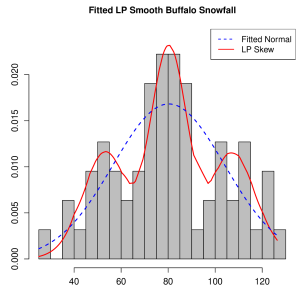
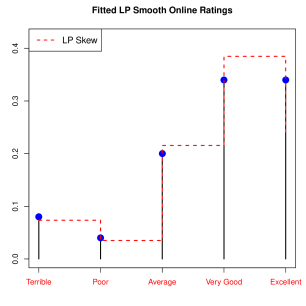
Figure 3: LP Skew density estimates. (a) Left; Buffalo Snowfall data. The baseline measure $\mathcal{N}(\mu=80.29,\sigma=23.72)$ shown in blue dotted line; (b) Right; Online rating data with base line measure as Poisson distribution with $\lambda=3.82$.

3.2.1 Smooth Density Modeling

Two examples are given to illustrate how LP skew smoothing methods nonparametrically identify the underlying probability law.

Figure 3(a) shows the Buffalo Snowfall data, previously analyzed by Parzen (1979). We select the normal distribution (with estimated mean $80.29$ and standard deviation $23.72$) as our baseline density $g(x)$. Data-driven AIC selects ${\widehat{d}}(u)=1-.337S_{6}(u)$. The resulting LP Skew estimate shown in Fig 3(a) strongly suggests tri-modal density.

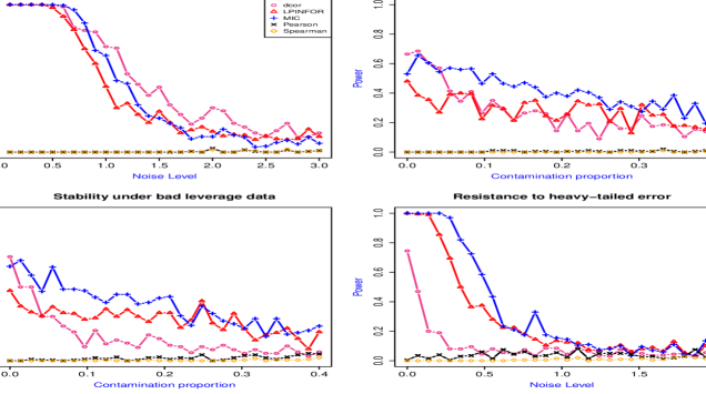
(a) Power curve for sine pattern

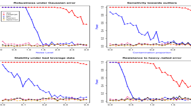
(b) Power curve for circle pattern

Figure 12: Estimated power curve for sine curve and circle pattern under four types of noise settings; set up described in Section 6.3.2

Fig 3(b) shows online rating discrete data from Tripadvisor.com of the Druk hotel with baseline model $g(x)$ being Poisson distribution with fitted $\lambda=3.82$. Data-driven AIC selects ${\widehat{d}}(u)=1-.55S_{2}(u)-.4S_{3}(u)+.23S_{4}(u)$. The estimated LP Skew probability estimates $\widehat{p}(x;x)$ captures the overall shape, including the two modes, which reflects the mixed customer reviews: (i) detects the sharp drop in probability of review being ‘poor’ (elbow shape); (ii) both peaks at the boundary, and (iii) finally, the “flat-tailed” shape at the end of the two categories (‘Very Good’ and ‘Excellent’). Compare our findings with Fig 12 of Sur et al. (2013), where they have used a substantially complex and computationally intensive model (Conway-Maxwell-Poisson mixture model), still fail to satisfactorily capture the shape of the discrete data.

3.2.2 General Goodness-of-fit Principle

LP Skew modeling naturally leads to a framework for distribution-free goodness-of-fit procedure, valid for mixed $X$ (discrete or continuous). A distribution-free goodness-of-fit framework for discrete data is comparatively much less developed and more challenging than continuous data (D’Agostino, 1986). Some recent attempts have been made by Best and Rayner (1999, 2003) and Khmaladze (2013).

To test whether the true underlying distribution $F$ equals $G$, we follow the following procedure:

Step A Estimate the ${\widehat{d}}(G(x))\,=\,1+\sum_{j}\operatorname{LP}[j;G,{\widetilde{F}}]\,T_{j}(x;G)$.

Step B Compute the goodness-of-fit test statistic $\int_{0}^{1}\widehat{d}^{2}\,-\,1\,=\,\sum_{j}\big{|}\operatorname{LP}[j;G,{\widetilde{F}}]\big{|}^{2}$. Justify the form of the test statistic by recognizing that under null the comparison distribution limit process $\sqrt{n}\big{[}\widetilde{D}(u;G,F)-u\big{]}\xrightarrow{D}B(u)$, Brownian Bridge for $0<u<1,$ with RKHS norm squared $\|h\|^{2}=\int_{0}^{1}|h^{\prime}(u)|^{2}\;\mathrm{d}u$.

The following result shows one remarkable equality between LP goodness-of-fit statistic and Chi squared statistic for discrete data.

Theorem 5.

For $X$ discrete with probable values $x_{j}$ and observe sample size $n$, one compares sample probabilities $\tilde{p}(x)$ with population model $p_{0}(x)$ by Chi-Squared statistic, which we represent by $n\operatorname{CHIDIV}$. Then LP goodness of fit statistics numerically equals to $\operatorname{CHIDIV}\big{[}p_{0}\,\|\,\tilde{p}\big{]}$.

To prove the result, verify the following:

$$\mbox{CHIDIV}\big{[}\,p_{0}\,\|\,\tilde{p}\big{]}\,=\,\sum_{x}p_{0}(x)\big{[}\tilde{p}(x)/p_{0}(x)\,-\,1\big{]}^{2}\,=\,\int_{0}^{1}\big{[}d(u;p_{0};\tilde{p})-1\big{]}^{2}\;\mathrm{d}u.$$ (3.4)

Chi-square statistic is a “raw-nonparametric” information measure, which we interpret by finding an approximately equal (numerically) “smooth” LP information measure with far fewer degrees of freedom because it is the sum of squares of only a few data-driven $\operatorname{LP}[j;G,{\widetilde{F}}]$. LP goodness-of-fit statistic for discrete distribution can be interpreted as Chi-square statistic with the fewest possible degrees of freedom that makes it more powerful. Our approach utilizes the automatic and universal algorithm to custom-construct orthonormal score polynomials of $F(X;X)$ for each given $X$; traditional methods construct orthonormal polynomials on a case-by-case basis by each time solving the heavy-duty Emerson recurrence (Emerson, 1968, Best and Rayner, 1999, 2003) relation, which could often be quite complicated for non-standard distributions.

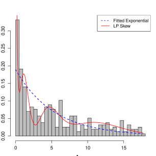
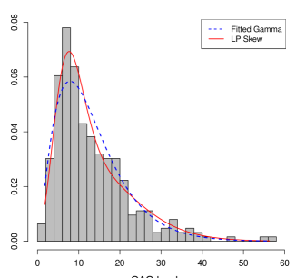
Figure 4: Goodness-of-fit of the marginal distributions of Ripley data.

Examples. For $Y=$ GAG level in Ripley data, we would like to investigate whether the parametric model Gamma fits the data. We select the Gamma distribution with shape $2.5$ and rate parameter $.19$ estimated from the data as our base line density $g(x)$. Estimated smooth comparison density is given by ${\widehat{d}}(u;G,F)=1+.16S_{3}(u)$, which indicates that the underlying probability model is slightly more skewed than the proposed parametric model. Fig 4(b) shows the final LP Skew estimated model.

For $X=$ AGE in Ripley data, we choose exponential distribution with estimated mean parameter $5.28$ as our $g(x)$. The estimated ${\widehat{d}}(u;G,F)=1+.32S_{2}(u)-.25S_{3}(u)-.22S_{5}(u)-.39S_{7}(u)$ with LP goodness-of-fit statistic as $\int{\widehat{d}}^{2}-1=0.365422$. Fig 4(a) shows that the exponential model is inadequate for capturing the plausible multi-modality and heavy-tail of age distribution.

3.2.3 Tail Alternative & Large-Scale Multiple Testing

We investigate the performance of the LP goodness-of-fit statistic under ‘tail alternative’ (detecting lack of fit “in the tail”). Consider the testing problem $H_{0}:F=\Phi$ verses Gaussian contamination model $H_{1}:F=\pi\Phi+(1-\pi)\Phi(\cdot-\mu)$, for $\pi\in(0,1)$ and $\mu>0$, which is critical component of multiple testing. It has been noted that traditional tests like Anderson–Darling (AD), Kolmogorov–Smirnov (KS) and Cramér-von Mises (CVM) lack power in this setting. We compare the performance of our statistic with four other statistics: AD, CVM, KS and Higher-criticism (Donoho and Jin, 2008). Fig 5 shows the power curve under different sparsity level $\pi=\{.01,.02,.05,.09\}$ where the signal strength $\mu$ varies from $0$ to $3.5$ under each setting, based on $n=5000$ sample size. We used 500 null simulated data sets to estimate the 95% rejection cutoff for all methods at the significance level $0.05$ and used $500$ simulated data sets from alternative to approximate the power. LP goodness-of-fit statistic does a satisfactory job of detecting deviations at the tails under a broad range of $(\mu,\pi)$ values, which is desirable as the true sparsity level and signal strength are unknown quantities. Application of this idea recently extended to modeling local false discovery rate in Mukhopadhyay (2013).

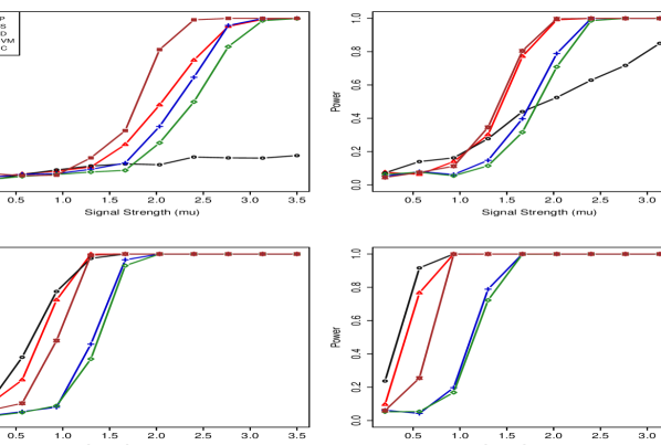
Figure 5: Power comparison of LP goodness-of-fit statistic under tail alternative (Section 3.2.3). The sparsity level changes $\pi=\{.01,.02,.05,.09\}$.

4 LP Copula Density Estimation

Copula density, pioneered by Sklar (1959) for continuous marginals, provides a general tool for dependence modeling. The copula density estimation problem is known to be a highly challenging problem, especially for discrete data as noted in Genest and Neslehova (2007) “A Primer on Copulas for Count Data.” Copula Distribution at $u=F(x;X),v=F(y;Y)$ for some $x,y$ is defined as

$$\operatorname{Cop}(u,v;X,Y)=F\big{(}Q(u;X),Q(v;Y);X,Y\big{)}.$$ (4.1)

For discrete and continuous $X$ and $Y$ define copula density for $0<u,v<1$ as

$$\operatorname{cop}(u,v;X,Y)\,=\,d(v;Y,Y|X=Q(u;X))\,=\,d(u;X,X|Y=Q(v;Y)),~{}0<u,v<1.$$ (4.2)

This section provides two fundamental nonparametric representations of copula density that hold for discrete and continuous marginals at the same time.

4.1 Representation and Estimation

Theorem 6 (LP Representation of Copula Density).

Square integrable copula density admits the following representation as infinite series of LP product score functions

$$\operatorname{cop}(u,v;X,Y)-1=\sum_{j,k>0}\operatorname{LP}(j,k;X,Y)\,S_{j}(u;X)\,S_{k}(v;Y),~{}0<u,v<1.$$ (4.3)

Equivalently,

$$\int_{[0,1]^{2}}\;\mathrm{d}u\;\mathrm{d}v\,d\big{[}v;Y,Y|X=Q(u;X)\big{]}\,S_{j}(u;X)\,S_{k}(v;Y)\,=\,\operatorname{LP}(j,k;X,Y).$$

A proof of copula LP representation is provided by representations of conditional copula density and conditional expectations:

$$d(v;Y,Y|X=Q(u;X)) = \sum_{k}S_{k}(v;Y)\,\mathbb{E}[T_{k}(Y;Y)|X=Q(u;X)]$$ (4.4)

$$\mathbb{E}[T_{k}(Y;Y)|X=Q(u;X)] = \sum_{j}S_{j}(u;X)\,\mathbb{E}[T_{j}(X;X)T_{k}(Y;Y)].$$ (4.5)

The LP copula representation provides data driven ‘smooth’ $L^{2}$ estimators of the copula density after constructing custom-built score functions and LP comoments.

We build the maximum entropy LP exponential copula density model based on the selected product score functions

$$\log\operatorname{cop}(u,v;X,Y)\,=\,\sum_{j,k>0}\theta_{j,k}\,S_{j}(u;X)\,S_{k}(v;Y)\,-\,K(\theta),\,\,~{}0<u,v<1.$$ (4.6)

We recommend plotting the slices of the copula along with the copula density for better insight into the nature of the dependence. Plot conditional comparison densities $d(v;Y,Y|X=Q(u;X))$ as a function of $v$ for selected values of $u$, also $d(u;X,X|Y=Q(v;Y))$ as a function of $u$ for selected values of $v$. The slices describes the conditional dependence of $X$ and $Y$, which will be utilized for correspondence analysis (in Section 5) and quantile regression (in Section 7).

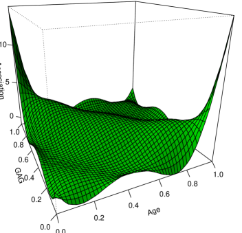
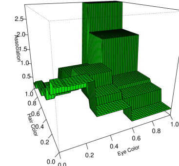
Figure 6: LP nonparametric copula density estimates for Ripley and Fisher data.

4.2 Example

Fig 6(a) displays the LP nonparametric copula estimate for the $(X,Y)$ Ripley data given by

$$\widehat{\operatorname{cop}}(u,v;X,Y)\,=\,1-0.91\,S_{1}(u)S_{1}(u)S_{1}(v)+0.71\,S_{2}(u)S_{2}(v)-0.59\,S_{3}(u)S_{3}(v)+0.42\,S_{4}(u)S_{4}(v)$$ (4.7)

For $(X,Y)$ discrete Fisher data ($4\times 5$ contingency table), the resulting smooth nonparametric checkerboard copula estimate is given by

$$\widehat{\operatorname{cop}}(u,v;X,Y)\,=\,1-0.423\,S_{1}(u)S_{1}(u)S_{1}(v)+0.157\,S_{2}(u)S_{2}(v)+0.115\,S_{2}(u)S_{1}(v),$$ (4.8)

shown in Fig 6(b). Note the piece-wise constant bivariate discrete smooth structure of the estimated copula density.

5 LP Canonical Copula Density Estimation

We present two more copula expansions (Karhunen-Loéve type expansion) that are valid for both discrete and continuous marginals. For $(X,Y)$ discrete, we show that the vast literature on dependence modeling of two-way contingency table (Goodman, 1991, 1996) can be elegantly unified by this formulation.

5.1 Representation and Estimation

Theorem 7 (LP Canonical Expansion of Copula Density).

Square integrable copula density admits the following two representations ($L^{2}$ and maximum entropy exponential model) based on the sequence of singular values of LP-comoment kernel $\lambda_{1}\geq\lambda_{2}\geq\cdots$ for $0<u,v<1$,

$$\operatorname{cop}(u,v) = 1+\sum_{k=1}^{\infty}\lambda_{k}\,\phi_{k}(u;X)\,\psi_{k}(v;Y),$$ (5.1)

$$\log\operatorname{cop}(u,v) = \sum_{k=1}^{\infty}\gamma_{k}\,\phi_{k}(u;X)\,\psi_{k}(v;Y)\,-\,K(\gamma).$$ (5.2)

Replace LP-comoment matrix appearing in Theorem 6 by its singular value decomposition (SVD) to get the required copula representation (5.1). Note that the singular values of the LP-comment matrix can be interpreted as the canonical correlation between the nonlinearly transformed random vectors $TX=(T_{1}(X;X),\ldots,T_{m}(X;X))^{\prime}$ and $TY=(T_{1}(Y;Y),\ldots,T_{m}(Y;Y))^{\prime}$. For this reason, we call this LP canonical copula representation.

For a $I\times J$ contingency table, the maximum number of terms in our LP copula expansion could be $\min(I,J)-1$. For $(X,Y)$ discrete Fisher data, the estimated LP canonical copula is given by $\operatorname{cop}(u,v)=1+.45\,\phi_{1}(u)\psi_{1}(v)+.17\,\phi_{2}(u)\psi_{2}(v)$.

Table 1: Fisher Data: Displayed joint probabilities $\Pr(X=x,Y=y)$ ; marginal probabilities $\Pr(X=x)$, $\Pr(Y=y)$; and corresponding mid-distributions, as well as coefficients of conditional comparison densities $d(v;Y,Y|X=x)$ and $d(u;X,X|Y=y)$.

	Hair Color
Eye Color	Fair	Red	Medium	Dark	Black	$p(x;X)$	$F^{\rm{mid}}(x;X)$	$\lambda_{1}\phi_{1}$	$\lambda_{2}\phi_{2}$
Blue	.061	.007	.045	.020	.001	.14	.07	-0.400	-0.165
Light	.128	.021	.108	.035	.001	.29	.28	-0.441	-0.088
Medium	.064	.016	.168	.076	.005	.33	.59	0.034	0.245
Dark	.018	.009	.075	.126	.016	.24	.88	0.703	-0.134
$p(y;Y)$	.27	.05	.40	.26	.02
$F^{\rm{mid}}(y;Y)$	.135	.295	.52	.85	.99
$\lambda_{1}\psi_{1}$	-0.544	-0.233	-0.042	0.589	1.094
$\lambda_{2}\psi_{2}$	-0.174	-0.048	0.208	-0.104	-0.286

5.2 Correspondence Analysis: LP Functional Statistical Algorithm

Given a $I\times J$ two-way contingency table, we seek to graphically display the association among the different row and column categories via correspondence analysis.

5.2.1 Algorithm

LP correspondence analysis algorithm can be described as follows: Step A Estimate LP canonical copula density (5.1) by performing SVD on LP-comoment matrix.

Step B Define the LP principal profile coordinates $\mu_{ik}=\lambda_{k}\phi_{k}(u_{i};X)$ and $\nu_{jk}=\lambda_{k}\psi_{k}(v_{j};Y)$.

Step C Jointly display the row and column profiles together in the same plot to get the LP correspondence map.

5.2.2 Example

Table 1 calculates the joint probabilities and the marginal probabilities of the Fisher data. The singular values of the estimated LP-comoment matrix are $0.446,0.173,0.029$. The rank-two approximation of LP canonical copula can adequately model (99.6%) the dependence. Table 1 computes the row and column scores using the aforementioned algorithm. Fig 7 shows the bivariate LP correspondence analysis of Fisher data, which displays the association between hair color and eye color.

5.2.3 LP Unification of Two Cultures

Our $L^{2}$ canonical copula-based row and column scoring (using LP algorithm) reproduces the classical correspondence analysis pioneered by Hirschfeld (1935) and Benzecri (1969). Alternatively, we could have used the LP canonical exponential copula model to calculate the row and column profiles by $\mu^{\prime}_{ik}=\gamma_{k}\phi_{k}(u_{i};X)$ and $\nu^{\prime}_{jk}=\gamma_{k}\psi_{k}(v_{j};Y)$, known as Goodman’s profile coordinates pioneered in Goodman (1981) and Goodman (1985), which leads to the graphical display sometimes known as a weighted logratio map (Greenacre, 2010) or the spectral map (SM) (Lewi, 1998). Our LP theory unifies the ‘two cultures’ of correspondence analysis, Anglo multivariate analysis (usual normal theory) and French multivariate analysis (matrix algebra data analysis), using LP representation theory of discrete checkerboard copula density.

Our $L^{2}$ canonical copula density (5.1) is sometimes known as correlation model or CA (Correspondence Analysis) model and the exponential copula model (5.2) as RC (Row-Col) association model (Goodman, 1991, 1996). Since our LP-scores satisfy: $\mathbb{E}[T_{j}(X;X)]=\sum_{i}T_{j}(x_{i};X)p(x_{i})=0$ and $\operatorname{Var}[T_{j}(X;X)]=\sum_{i}T^{2}_{j}(x_{i};X)p(x_{i})=1$ by construction, this association model also known as the weighted RC model.

5.2.4 Functional Statistical Interpretation

Orthogonal $L^{2}$ coefficients of the piece-wise constant conditional copula densities (slices of copula density) of our canonical copula model satisfies:

$$\operatorname{LP}[k;Y,Y|X=Q(u;X)] = \lambda_{k}\,\phi_{k}(u;X),$$ (5.3)

$$\operatorname{LP}[k;X,X|Y=Q(v;Y)] = \lambda_{k}\,\psi_{k}(v;X).$$ (5.4)

This implies that the LP correspondence scores capture the shape of piece-wise constant conditional copula density functions. Thus, our correspondence analysis algorithm can be interpreted as comparing the ‘similarity of the shapes of conditional comparison density functions’ (captured by orthogonal coefficients) of row categories with column categories, as shown in the Fig 8 for Fisher data.

5.2.5 Low-Rank Smoothing Model, Smart Computational Algorithm

All currently available methods perform singular value decomposition on raw distance matrix (also known as contingency ratios) $\operatorname{cop}(F(x),F(y))=p(x,y;X,Y)/p(x;X)p(y;Y)$ or $\log[\operatorname{cop}(F(x),F(y))]$, which is of the order $I\times J$; this can have prohibitively high computational complexity and storage requirements for very large $I$ and $J$. Moreover, this is numerically unstable for sparse tables.

On the other hand, LP algorithm performs correspondence analysis by SVD on LP comoment matrix, which is often a far smaller order than the dimensional of the observed frequency matrix. Thus, our algorithm provides efficient ways of compressing the structure of large tables. For the structured contingency table, the spectrum of “raw” contingency ratio matrix can be approximated by the spectrum of “smooth” LP-comoment matrix, which could provide enormous computational gain for large data.

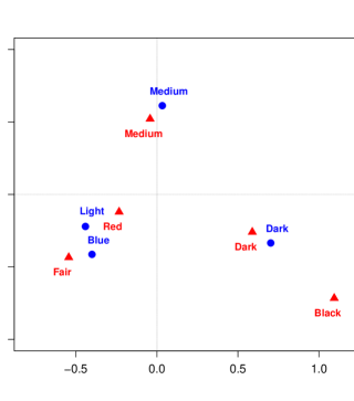
Figure 7: (color online) LP correspondence map for Fisher Hair and Eye color data

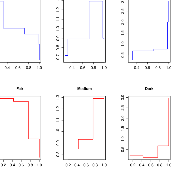
Figure 8: (color online) Correspondence analysis matches the shapes of conditional comparison density of row categories (blue) with column categories (red). See the similarity of the shapes of row and comumn categoriess and matches with the findings in Fig 7

5.3 Interpretation: $2\times 2$ Table

We establish connection between the parameters of our LP copula models and traditional statistical measures for $2\times 2$ table. Our approach provides an alternative elegant derivation presented in Gilula et al. (1988) and Goodman (1991).

Theorem 8.

For $2\times 2$ contingency table with Pearson correlation $\phi$ and odds-ratio $\delta$,

$$\lambda_{1} = \big{|}\operatorname{LP}[1,1;X,Y]\big{|}\,\,=\,\,\big{|}\phi(X,Y)\big{|}$$ (5.5)

$$\gamma_{1} = \big{|}\theta_{1,1}\big{|}\,\,=\,\,\big{|}\log\delta\big{|}\big{(}P_{1+}P_{+1}P_{2+}P_{+2}\big{)}^{1/2}$$ (5.6)

To prove the result first verify that

$$T_{1}(0;X)=-\sqrt{P_{2+}/P_{1+}}, T_{1}(1;X)=\sqrt{P_{1+}/P_{2+}}$$

$$T_{1}(0;Y)=-\sqrt{P_{+2}/P_{+1}}, T_{1}(1;Y)=\sqrt{P_{+1}/P_{+2}},$$ (5.7)

where $P_{i+}=\sum_{j}P_{ij}$ and $P_{+j}=\sum_{i}P_{ij}$, and $P_{ij}$ denotes the $2\times 2$ probability table. We then have the following,

$$\operatorname{LP}[1,1;X,Y] = \mathbb{E}[T_{1}(X;X)T_{1}(Y;Y)]\,=\,\sum_{i=1}^{2}\sum_{j=1}^{2}P_{ij}T_{1}(i-1;X)\,T_{1}(j-1;Y)$$ (5.8)

$$= \Big{[}P_{11}(P_{2+}P_{+2})-P_{12}(P_{2+}P_{+1})-P_{21}(P_{1+}P_{+2})+P_{22}(P_{1+}P_{+1})\Big{]}/\big{(}P_{1+}P_{+1}P_{2+}P_{+2}\big{)}^{1/2}$$

$$= \big{(}P_{11}P_{22}-P_{12}P_{21}\big{)}/\big{(}P_{1+}P_{+1}P_{2+}P_{+2}\big{)}^{1/2}\,=\,\phi(X,Y).$$

To prove (5.6) verify that

$$\theta_{1,1} = \int\log\big{[}\operatorname{cop}(u,v)\big{]}S_{1}(u;X)S_{1}(v;Y)\;\mathrm{d}u\;\mathrm{d}v$$ (5.9)

$$= \sum_{i=1}^{2}\sum_{j=1}^{2}\log\left[\dfrac{P_{ij}}{P_{i+}P_{+j}}\right]\,T_{1}(i-1;X)\,T_{1}(j-1;Y)\,P_{i+}\,P_{+j}$$

$$= \log\left[\dfrac{P_{11}P_{22}}{P_{12}P_{21}}\right]\,\big{(}P_{1+}P_{+1}P_{2+}P_{+2}\big{)}^{1/2}.$$

6 LPINFOR Dependence Measure

Computationally fast copula-based nonparametric dependence measure LPINFOR and its properties are discussed in this section. We present two decompositions of LPINFOR, which allow finer understanding of the dependence between $X$ and $Y$ from two different perspectives. Applications to nonlinear dependence modeling and sparse contingency table are considered. A comparative simulation study is also provided.

6.1 Definition, Properties and Interpretation

Dependence of $X$ and $Y$ can be nonparametrically measured by

$$\operatorname{LPINFOR}(X,Y)~{}=~{}\sum_{j,k>0}\big{|}\operatorname{LP}[j,k;X,Y]\big{|}^{2}~{}=~{}\iint_{[0,1]^{2}}\big{[}\operatorname{cop}(u,v;X,Y)-1\big{]}^{2}\;\mathrm{d}u\;\mathrm{d}v.$$ (6.1)

The second equality follows from LP copula representation (4.3) by applying Parseval’s identity. Summing over significant indices $j,k$ gives a smooth estimator of $\operatorname{LPINFOR}(X,Y)$. The power of this method is best described by its applications, which are presented in the next section. The name LPINFOR is motivated from the observation that it can be interpreted as an INFORmation-theoretic measure belonging to the family of Csiszar’s f-divergence measures (Csiszár, 1975). LPINFOR is simultaneously a global correlation index and a directional statistic whose components capture the ways in which the copula density deviates from uniformity. By construction, LPINFOR is invariant to monotonic transformations of the two variables.

An alternative representation of LPINFOR can be derived from the singular value decomposition representation (5.1) as $\operatorname{LPINFOR}(X,Y)=\sum_{k}\lambda^{2}_{k}$. Note that our measure works for discrete or continuous marginals. LPINFOR, under two important cases (bivariate normal and contingency table), are described in the next result.

Theorem 9 (Properties).

Two important properties for LPINFOR measure (i) For $(X,Y)$ bivariate normal $\operatorname{LPINFOR}$ is an increasing function of $|\rho|$:

$$\operatorname{LPINFOR}(X,Y)\,=\,\dfrac{\rho^{2}}{1-\rho^{2}}.$$ (6.2)

(ii) For $(X,Y)$ forming a $I\times J$ contingency table we have

$$\operatorname{LPINFOR}(X,Y)\,=\,\operatorname{CHIDIV}(X,Y)\,=\,\chi^{2}/n.$$ (6.3)

Part (i): To compute the integral $\int\big{[}\operatorname{cop}(u,v)-1\big{]}^{2}du\,dv$ for Gaussian copula, a quantity that is invariant to the choice of orthonormal polynomials, we first switch orthogonal polynomials from LP- orthonormal score functions to Hermite polynomials and use the following well-known result to complete the proof.

Lemma 9.1 (Eagleson, 1964 and Koziol, 1979).

Let $H_{j}(x)$ denotes the $j$th orthonormalized Hermite polynomial. For bivariate Gaussian copula with correlation parameter $\rho$ we have the following inner-product result:

$$\iint_{[0,1]^{2}}\dfrac{\phi[\Phi^{-1}(u;X),\Phi^{-1}(v;Y);\rho]}{\phi[\Phi^{-1}(u;X)]\,\phi[\Phi^{-1}(v;Y)]}\,H_{j}[\Phi^{-1}(u;X)]\,H_{k}[\Phi^{-1}(v;Y)]\;\mathrm{d}u\;\mathrm{d}v\,=\,\rho^{j}\,\mathbb{I}[j=k].$$

Part(ii): Note that for $(X,Y)$ discrete, $\operatorname{cop}(F(x),F(y);X,Y)=p(x,y;X,Y)/p(x;Y)p(y;Y)$. Verify the following representation to complete the proof

$$\operatorname{CHIDIV}(X,Y)\,=\,\chi^{2}/n\,=\,\sum_{x,y}\,p(x;Y)\,p(y;Y)\big{[}\operatorname{cop}\big{(}F(x),F(y);X,Y\big{)}-1\big{]}^{2}.$$ (6.4)

Example. For the Ripley data we previously computed the LP-comoment matrix (2.8). The smooth LPINFOR (taking sum of squares of the significant elements denoted by ‘^∗’) dependence number is $1.851$. There is strong evidence of nonlinearity due to the presence of higher-order LP-comoments. Coefficient of linearity can be defined as $|\operatorname{LP}[1,1]|^{2}/\operatorname{LPINFOR}=.45$. Other applications of LPINFOR as a nonlinear correlation measure will be investigated in Section 6.3.2.

For Fisher data, the chisquare divergence or total inertia: $\chi^{2}/n$=.230 with df $(4-1)\times(5-1)=12$, and the smooth-LPINFOR dependence number is $.220$, with much fewer degrees of freedom $3$ (2.9). LPINFOR numerically computes the ‘raw’ chisquare divergence number but the computation of degrees of freedom is different. In our case, degrees of freedom dramatically drops from the usual $12$ to $3$, which boosts the power of our method. Applicability for large sparse tables is described in Section 6.3.1.

6.2 Conditional LPINFOR, Interpretation

Define conditional LPINFOR

$$\operatorname{LPINFOR}(Y|X=x)\,=\,\int_{0}^{1}\big{[}d\left(v;\,Y,Y|X=x\right)\,-\,1\big{]}^{2}\;\mathrm{d}v\,=\,\sum_{k>0}\big{|}\operatorname{LP}[k;Y,Y|X=x]\big{|}^{2}.$$ (6.5)

The components $\operatorname{LP}[k;Y,Y|X=x]=\mathbb{E}[T_{k}(Y;Y);Y|X=x]$ computed from LP-comoments by

$$\operatorname{LP}[k;Y,Y|X=x]~{}=~{}\sum_{j>0}\operatorname{LP}[j,k;X,Y]\,T_{j}(x;X).$$

The LPINFOR can be decomposed as

$$\operatorname{LPINFOR}(X,Y)~{}=~{}\int\operatorname{LPINFOR}(Y|X=x)\;\mathrm{d}F(x;X)$$ (6.6)

The conditional LPINFOR quantifies the effect of different levels of $X$ on $Y$. For $(X,Y)$ two-way continency table the components of conditional LPINFOR $\operatorname{LP}[k;Y,Y|X=x]$ provide the LP profile coordinates for correspondence analysis (Section 5.2). For $(X,Y)$ continuous these components give insight how the shape of conditional density $f(y;Y|X=x)$ changes with the levels of the covariate $X$, illustrated in Section 7.4.

6.3 Applications

6.3.1 Sparse Contingency Table

Consider the example shown in Table 2. Our goal is to understand the association between Age and Intelligence Quotient (IQ). It is well known that the accuracy of chi-squared approximation depends on both sample size $n$ and number of cells $p$. Classical association mining tools for contingency tables like Pearson chi-squared statistic and likelihood ratio statistic break down for sparse tables (where many cells have observed zero counts, see Haberman (1988)) - a prototypical example of “large $p$ small $n$” problem.

The classical chi-square statistic yields test statistic = $60$, df = $56$, p-value = $0.3329$, failing to capture the pattern from the sparse table. Eq 6.7 computes the LP-comoment matrix. The significant element is $\operatorname{LP}[2,1]=-0.617$, with the associated p-value $0.0167$. LPINFOR thus adapts successfully to sparse tables.

Table 2: Wechsler Adult Intelligence Scale (WAIS) by males of various ages. Is there any pattern ? Data described in Mack and Wolfe (1981) and Rayner and Best (1996).

	Intelligence Scale
Age group	1	2	3	4	5	6	7	8	9	10	11	12	13	14	15
$16-19$	0	1	0	0	0	0	0	1	0	1	0	0	0	0	0
$20-34$	0	0	0	0	0	1	0	0	0	0	1	0	0	1	0
$35-54$	0	0	0	0	0	0	0	0	1	0	0	0	1	0	1
$55-69$	0	0	1	0	0	0	1	0	0	0	0	1	0	0	0
$69+$	1	0	0	1	1	0	0	0	0	0	0	0	0	0	0

$$\widehat{\operatorname{LP}}\big{[}X={\rm Age},Y={\rm IQ}\big{]}~{}=~{}\begin{bmatrix}-0.316&0.173&0.168&-0.114\\[3.80005pt] -0.618^{*}&-0.031&-0.101&0.068\\[3.80005pt] 0.087&0.136&0.077&0.037\\[3.80005pt] 0.165&0.215&0.042&0.289\\[3.80005pt] \end{bmatrix}$$ (6.7)

The higher-order significant $\operatorname{LP}[2,1;X,Y]=\mathbb{E}[T_{2}(X;X)T_{1}(Y;Y)]$ comoment not only indicates strong evidence of non-linearity but also gives a great deal of information regarding the functional relationship between age and IQ. Our analysis suggests that IQ is associated with the $T_{2}(X;X)$ that has a quadratic (more precisely, inverted U-shaped) age effect, which agrees with all previous findings that IQ increases as a function of age up to a certain point, and then it declines with increasing age. This example also demonstrates how the LP-comoment based approach nonparametrically finds the optimal non-linear transformations for two-way contingency tables, extending Breiman and Friedman (1985)

$$\rho\big{(}\Psi^{*}(Y),\,\Upsilon^{*}(X)\big{)}~{}=~{}\max_{\Psi,\phi}\rho\big{(}\Psi(Y),\,\Upsilon(X)\big{)}.$$

6.3.2 Nonlinear Dependence Measure, Power Comparison

We compare the power of our LPINFOR statistic with distance correlation (Székely and Rizzo, 2009), maximal information coefficient (Reshef et al., 2011), Spearman and Pearson correlation for testing independence under six different functional relationships (for brevity we restrict our attention to the relationships shown in Fig 9) and four different types of noise settings: (i) $E_{1}:$ Gaussian noise $\mathcal{N}(0,\sigma)$ where $\sigma$ varying from $0$ to $3$; (ii) $E_{2}:$ Contaminated Gaussian $(1-\eta)\mathcal{N}(0,1)+\eta\mathcal{N}(1,3)$, where the contamination parameter $\eta$ varies from $0$ to $.4$; (iii) $E_{3}:$ Bad leverage points are introduced to the data by $(1-\eta)\mathcal{N}(0,1)+\eta\mathcal{N}(\mu,1)$, where $\mu=\{\pm 20,\pm 40\}$ w.p $1/4$ and $\eta$ varies from $0$ to $.4$; (iv) $E_{4}:$ heavy-tailed noise is introduced via Cauchy distribution with scale parameter that varies from $0$ to $2$.

Table 3: Performance summary table on the basis of empirical power among six competing methods, compared over six bivariate relationships and four different noise settings.

		Functional Relation
Noise	Performance	Linear	Quadratic	Lissajous	W-shaped	Sine	Circle
$E_{1}$	Winner	Pearson	LPINFOR	LPINFOR	Dcor	Dcor	LPINFOR
	Runner-up	Spearman	Dcor	MIC	LPINFOR	MIC	MIC
$E_{2}$	Winner	Spearman	LPINFOR	LPINFOR	LPINFOR	MIC	LPINFOR
	Runner-up	Dcor	MIC	MIC	Dcor	Dcor	MIC
$E_{3}$	Winner	Spearman	LPINFOR	LPINFOR	LPINFOR	MIC	LPINFOR
	Runner-up	LPINFOR	MIC	MIC	MIC	LPINFOR	MIC
$E_{4}$	Winner	Spearman	LPINFOR	LPINFOR	LPINFOR	MIC	LPINFOR
	Runner-up	LPINFOR	MIC	Dcor	MIC	LPINFOR	MIC

The simulation is carried out based on sample size $n=300$. We used $250$ null simulated data sets to estimate the 95% rejection cutoffs for all methods at the significance level $0.05$ and used $200$ simulated data sets from alternative to approximate the power, similar to Noah and Tibshirani (2011). We have fixed $m=4$ to compute LPINFOR for all of our simulations. Fig 10-12 show the power curves for the bivariate relations under four different noise settings. We summarize the findings in Table 3, which provides strong evidence that LPINFOR performs remarkably well across s wide-range of settings.

Figure 9: Various functional relationships considered in our simulation study in Section 6.3.2.

Computational Considerations. We investigate the issue of scalability to large data sets (big $n$ problems) for the three competing nonlinear correlation detectors: LPINFOR, distance correlation (Dcor), and maximal information coefficient (MIC). Generate $(X,Y)\sim\mbox{Uniform}[0,1]^{2}$ with sample size $n=20,50,100,500,1000,5000$ $,10,000$. Table 5 reports the average time in sec (over $50$ runs) required to compute the corresponding statistic. It is important to note the software platforms used for the three methods: DCor is written in JAVA, MIC is written in C, and we have used (unoptimized) R for LPINFOR. It is evident that for large sample sizes both Dcor and MIC become almost infeasible - not to mention computationally extremely expensive. On the other hand, LPINFOR emerges clearly as the computationally most efficient and scalable approach for large data sets.

Table 4: Computational Complexity: uniformly distributed, independent samples of size $n$, averaged over $50$ runs based on Intel(R) Core(TM) i7-3540M CPU @ 3.00GHz 2 Core(s) processor. Timings are reported in seconds.

Methods	Size of the data sets
	$n=100$	$n=500$	$n=1000$	$n=2500$	$n=5000$	$n=10,000$
LPINFOR	0.002 (.004)	0.001 (.004)	0.002 (.005)	0.005 (.007)	0.011 (.007)	0.018 (.007)
Dcor	0.003 (.007)	0.094 (.013)	0.371 (.013)	1.773 (.450)	7.756 (.810)	44.960 (12.64)
MIC	0.312 (.007)	0.628 (.008)	1.357 (.035)	5.584 (.110)	19.052 (.645)	65.170 (2.54)

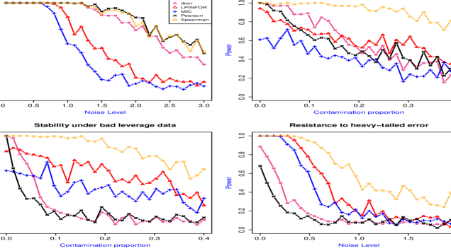
(a) Power curve for linear pattern

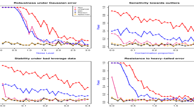
(b) Power curve for quadratic pattern

Figure 10: Estimated power curve for linear and quadratic pattern under four types of noise settings; set up described in Section 6.3.2

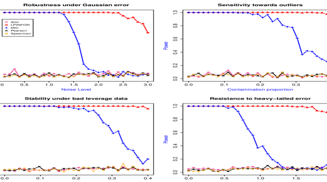
(a) Power curve for Lissajous curve

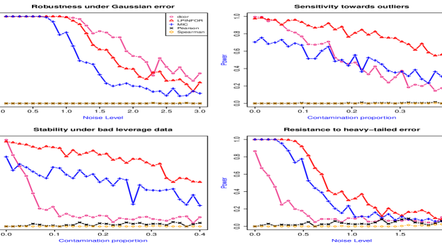
(b) Power curve for W-pattern

Figure 11: Estimated power curve for Lissajous curve and W-pattern under four types of noise settings; set up described in Section 6.3.2

7 LPSmoothing (X,Y)

We propose a nonparametric copula-based conditional mean and conditional quantile modeling algorithm. We introduce LP zero-order comoments (defined for discrete and continuous marginals) as the regression coefficients of our nonparametric model (generalizing Gini correlation Schechtman and Yitzhaki (1987) and Serfling and Xiao (2007)). An illustration using Ripley data is also given, demonstrating the versatility of our approach.

7.1 Copula-Based Nonparametric Regression

Theorem 10.

Conditional expectation $\mathbb{E}[Y|X=x]$ can be approximated by linear combination of orthonormal LP-score functions $\{T_{j}(X;X)\}_{1\leq j\leq m}$ with coefficients defined as $\mathbb{E}\big{[}\mathbb{E}[Y|X]T_{j}(X;X)\big{]}=\mathbb{E}[YT_{j}(X;X)]=\operatorname{LP}(j,0;X,Y)$, because of the representation:

$$\mathbb{E}\big{[}Y\mid X=x\big{]}-\mathbb{E}[Y]\,=\,\sum_{j>0}T_{j}(x;X)\operatorname{LP}(j,0;X,Y).$$ (7.1)

Direct proof uses $\mathbb{E}\big{[}(Y-\mathbb{E}[Y|X])T_{j}(X;X)\big{]}=0$ for all $j$, and Hilbert space theory. An alternative derivation of this representation is given below, which elucidates the connection between copula-based nonlinear regression. Using LP-representation of copula density (4.3), we can express conditional expectation as

$$\mathbb{E}[Y|X=x] = \int y\operatorname{cop}\big{(}F(x),F(y)\big{)}\;\mathrm{d}F(y)\,=\,\int y\Big{[}1+\sum_{j,k>0}\operatorname{LP}[j,k;X,Y]\,T_{j}(x;X)\,T_{k}(y;Y)\Big{]}\;\mathrm{d}F(y)$$ (7.2)

$$= \mathbb{E}[Y]~{}+~{}\sum_{j>0}T_{j}(x;X)\,\left\{\sum_{k>0}\operatorname{LP}[j,k;X,Y]\,\operatorname{LP}[k;Y]\right\}.$$

Compete the proof by recognizing

$$\operatorname{LP}[j,0;X,Y]\,=\,\mathbb{E}\Big{[}\,\mathbb{E}\big{[}T_{j}(X;X)|Y\big{]}Y\,\Big{]}\,=\,\sum_{k>0}\operatorname{LP}[j,k;X,Y]\,\operatorname{LP}[k;Y].$$

Our approach is an alternative to parametric copula-based regression model (Noh et al., 2013, Nikoloulopoulos and Karlis, 2010). Dette et al. (2013) aptly demonstrated the danger of the “wrong” specification of a parametric family even in one or two dimensional predictor. They noticed commonly used parametric copula families are not flexible enough to produce non-monotone regression function, which makes it unsuitable for any practical use. Our LP nonparametric regression algorithm yields easy to compute closed form expression (7.1) for conditional mean function, which bypasses the problem of misspecification bias and can adapt to any nonlinear shape. Moreover, our approach can easily be integrated with data-driven model section criterions like AIC or Mallow’s $C_{p}$ to produce a parsimonious model.

7.2 Generalized Gini Correlations as Zero Order LP-Comoments

In this section We establish connection between the Zero-order LP-comoments (regression coefficients) and Gini correlation (Schechtman and Yitzhaki, 1987) .

Generalized LP-Gini Correlations. Define the Generalized Gini correlations by

$$R_{\rm{GINI}}(j;Y|X) = \operatorname{LP}(j,0;X,Y)/\operatorname{LP}(j,0;Y,Y)=\mathbb{E}[T_{j}(X;X)Y]/\mathbb{E}[T_{j}(Y;Y)Y]$$

$$R_{\rm{GINI}}(k;X|Y) = \operatorname{LP}(0,k;X,Y)/\operatorname{LP}(0,k;X,X)=\mathbb{E}[T_{k}(Y;Y)X]/\mathbb{E}[T_{k}(X;X)X]$$

LP-comoment representation of traditional Gini correlation $R_{\rm{GINI}}(1;Y|X)$ and $R_{\rm{GINI}}(1;X|Y)$. We extend the classical Gini correlation concept in at least two major directions: (i) our definition, unlike previous versions, is well-defined for both discrete and continuous variables. As noted in Chapter 2 of Yitzhaki and Schechtman (2013) to extend the concept of Gini for discrete random variables requires not-trivial adjustments, which are already incorporated in our LP-Gini algorithm. (ii) We provide non-linear generalizations (defined for $j\geq 1$) of classical Gini correlation using higher-order LP-score functions.

Next we investigate some useful properties of LP-Gini correlation for bivariate normal that can be used for quick diagnostic purpose.

Theorem 11.

For $(X,Y;\rho)$ Bivariate Normal we have the following relationship

$$\operatorname{LP}[j,0;X,Y]\,=\,\rho\,\operatorname{LP}[j,0;Y,Y],~{}~{}\mbox{and}~{}~{}\operatorname{LP}[j,0;Y,X]\,=\,\rho\,\operatorname{LP}[j,0;X,X].$$

To prove the Theorem 11 note that, for bivariate normal, $\mathbb{E}(Y|X)=\mu_{y}+\rho\,\sigma(y)\,X$ (w.l.g we can assume $X$ has mean $0$ and variance $1$ as it only appear as a function of ranks in Gini expression $R_{\rm{GINI}}(j;Y|X)$). For $Z\sim\mathcal{N}(0,1)$ we then have

$$\mathbb{E}[YT_{j}(X)]=\mathbb{E}\big{[}\mathbb{E}[Y|X]T_{j}(X)\big{]}=\rho\,\sigma(y)\operatorname{LP}[0,j;Z,Z].$$ (7.3)

Finally, observe $\operatorname{LP}[j,0;Y,Y]=\sigma(y)\operatorname{LP}[0,j;Z,Z]$ to complete the proof.

Corollary 11.1.

For $(X,Y;\rho)$ Bivariate Normal we have the following important property

$$R_{\rm{GINI}}[j;Y|X]\,=\,R_{\rm{GINI}}[j;X|Y]\,=\,\rho,~{}\mbox{for all}\,\,j\,\mbox{odd}.$$

As a special case of Corollary 11.1 we derive that the co-Ginis $R_{\rm{GINI}}(1;Y|X)$ and $R_{\rm{GINI}}(1;X|Y)$ are equal to $\rho$ for bivariate normal (Yitzhaki and Schechtman, 2013).

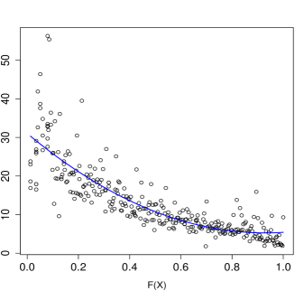
(a) Conditional Mean

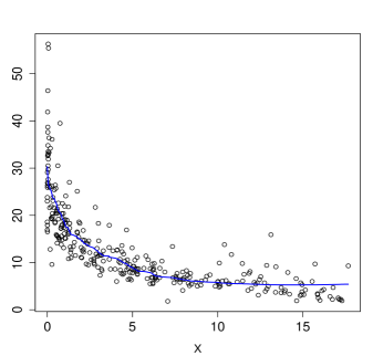
(b) Conditional Mean

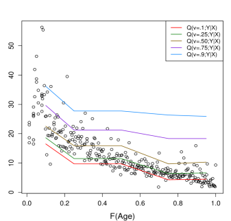
(c) Conditional Quantile

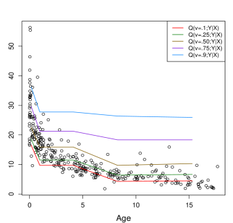
(d) Conditional Quantile

Figure 13: (color online) Smooth nonparametric copula based nonlinear regression. Conditional quantile

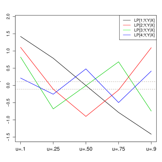
Figure 14: (color online) Conditional LPINFOR curve and its component decomposition for Ripley data.

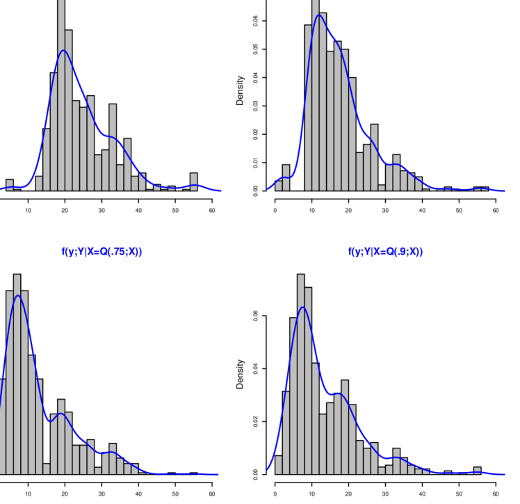
Figure 15: The estimated nonparametric conditional distributions $f(y;Y|X=Q(u;X))$ for $u=.1,.25,.75,.9$.

7.3 Conditional Distribution, Conditional Quantile

Given $(X,Y)$, it is often of interest to estimate the conditional quantiles and conditional density for comprehensive insight. Our nonparametric estimation of conditional density $f(y;Y|X=x)$ is based on the following LP Skew modeling for $x,y\in{\mathbb{R}}$

$$f(y;Y|X=x)\,=\,f(y;Y)\operatorname{cop}(F(x;X),F(y;Y))\,=\,f(y;Y)\,d\big{(}F(y;Y);Y,Y|X=x\big{)}.$$ (7.4)

LP copula estimation theory (presented in Section 4) allows simultaneous estimation of all the copula slices or conditional comparison densities $d(v;Y|X=Q(u;X))$ for various $u$.

Conditional quantiles $Q(v;Y,Y|X=Q(u;X))$ can be simulated by accept-reject sampling from conditional comparison density. Our approach generalizes the seminal work by Koenker and Bassett (1978) on parametric (linear) quantile regression to nonparametric nonlinear setup, which guaranteed to produce non-crossing quantile curves (a longstanding practical problem, see Koenker (2005), He (1997) for details).

7.4 Example

A comprehensive analysis of the Ripley data is presented using LP algorithmic modeling. Our goal is to answer the scientific question of Ripley data based on $n=314$ sample,: what are normal levels of GAG in children of each age between $1$ and $18$ years of age. In the following, we describe the steps of LP nonparametric algorithm.

Step A. Ripley (2004) discusses various traditional regression modeling approaches using polynomial, spline, local polynomials. Figure 13(a,b) displays estimated LP nonparametric (copula based) conditional mean $\mathbb{E}[Y|X=x]$ function (7.1) given by:

$$\widehat{\mathbb{E}}[Y|X=x]\,=\,13.1-7.32\,T_{1}(x)+2.20\,T_{2}(x).$$

Step B. We simulate the conditional quantiles from the estimated conditional comparison densities (slices of copula density), and the resulting smooth nonlinear conditional quantile curves $Q(v;Y,Y|X=Q(u;X))$ are shown in Fig 13(c,d) for $u=.1,.25,.5,.75,.9$. Recall from Fig 4 that the marginal distributions of $X$ (age) and $Y$ (GAG levels) are highly skewed and heavy tailed, which creates a prominent sparse region at the “tail” areas. Our algorithm does a satisfactory job in nonparametrically estimating the extreme quantile curves under this challenging scenario. We argue that these estimated quantile regression curves provide the statistical solution to the scientific question: what are “normal levels” of GAG in children of each age between $1$ and $18$? Step C. Conditional LPINFOR curve is shown in Fig 14(a). The decomposition of conditional LPINFOR into the components describes the shape of conditional distribution changes, as shown in Fig 14(b). For example, $\operatorname{LP}[1;Y,Y|X=Q(u;X)]$ describes the conditional mean, $\operatorname{LP}[2;Y,Y|X=Q(u;X)]$ the conditional variance, and so on. Tail behaviour of the conational distributions seem to change rapidly as captured by the $\operatorname{LP}[4;Y,Y|X=Q(u;X)]$ in Fig 14(b). Step D. The estimated conditional distributions $f(y;Y|X=Q(u;X))$ are displayed in Fig 15 for $u=.1,.25,.75,.9$. Conditional density shows interesting bi-modality shape at the extreme quantiles. It is also evident from Figure 15 that the classical location-scale shift regression model is inappropriate for this example, which necessitates going beyond the conditional mean description for modeling this data that can tackle the non-Gaussian heavy-tailed data.

Appendix

A1. Shifted Orthonormal Legendre Polynomials

Orthonormal Legendre polynomials $\operatorname{Leg}_{j}(u)$ on interval $0<u<1$

$$\operatorname{Leg}_{0}(u) = 1$$

$$\operatorname{Leg}_{1}(u) = \sqrt{12}(u-.5)$$

$$\operatorname{Leg}_{1}(u) = \sqrt{5}(6u^{2}-6u+1)$$

$$\operatorname{Leg}_{3}(u) = \sqrt{7}(20u^{3}-30u^{2}+12u-1)$$

$$\operatorname{Leg}_{4}(u) = 3(70u^{4}-140u^{3}+90u^{2}-20u+1)$$

$$\vdots$$

A2. Proof of Lemma 2.1

To prove $Q(F(X))=X$ with probability $1$. Call $u$ probable if there exists $x$ such that $F(x;X)=u$. Define $x(u)$ to be smallest $x$ satisfying $F(x;X)=u$. Verify $Q(F(x(u)))=x(u)$ for $u$ probable. With probability $1$ the observed value of $X$ belongs to $\{x:x=x(u)\}$ for some $u$ probable. Therefore with probability $1$, $Q(F(X))=X$.

A3. Table of LP Moments

Table 5 shows LP moments for some standard discrete and continuous distributions.

Table 5: LP Moments of standard distributions.

	LP Moments
Distribution	$\operatorname{LP}[1;X]$	$\operatorname{LP}[2;X]$	$\operatorname{LP}[3;X]$	$\operatorname{LP}[4;X]$	$\operatorname{LP}[5;X]$	$\operatorname{LP}[6;X]$
Poisson$(\lambda=2)$	1.371	0.205	0.225	0.110	0.103	0.073
Geometric$(p=0.2)$	3.880	1.668	0.985	0.670	0.493	0.381
Uniform$[0,1]$	0.289	0	0	0	0	0
Standard Normal	0.977	0	0.183	0	0.081	0
Student’s t-df $2$	1.926	0	1.104	0	0.866	0
Chi-squared-df $4$	2.598	0.787	0.562	0.324	0.268	0.187

A4. Table of LP Comoments

LP-comoment matrix of order $m=4$ is displayed in the following equation for bivariate standard normal distribution with $\rho=0,.5,.9$.

$$\begin{bmatrix}0.0&0.0&0.0&0.0\\ 0.0&0.0&0.0&0.0\\ 0.0&0.0&0.0&0.0\\ 0.0&0.0&0.0&0.0\end{bmatrix}\hskip 20.00003pt\begin{bmatrix}0.48&0.0&0.07&0.0\\ 0.0&0.20&0.0&0.07\\ 0.07&0.0&0.08&0.0\\ 0.0&0.07&0.0&0.0\end{bmatrix}\hskip 20.00003pt\begin{bmatrix}0.89&0.0&0.04&0.0\\ 0.0&0.76&0.0&0.09\\ 0.04&0.0&0.61&0.0\\ 0.0&0.09&0.0&0.47\end{bmatrix}$$

$\hskip 50.00008pt\rho=0\hskip 100.00015pt\rho=.5\hskip 100.00015pt\rho=.9\hskip 45.00006pt$

References

- Benzecri (1969) Benzecri, J. P. (1969). Statistical analysis as a tool to make patterns emerge from data. New York: Academic Press.
- Best and Rayner (1999) Best, D. and J. Rayner (1999). Goodness of fit for the poisson distribution. Statistics & probability letters 44(3), 259–265.
- Best and Rayner (2003) Best, D. and J. Rayner (2003). Tests of fit for the geometric distribution. Communications in Statistics-Simulation and Computation 32(4), 1065–1078.
- Blumentritt and Schmid (2012) Blumentritt, T. and F. Schmid (2012). Nonparametric estimation of copula-based measures of multivariate association from contingency tables. Journal of Statistical Computation and Simulation (ahead-of-print), 1–17.
- Breiman and Friedman (1985) Breiman, L. and J. H. Friedman (1985). Estimating optimal transformations for multiple regression and correlation. Journal of the American Statistical Association 80(391), 580–598.
- Csiszár (1975) Csiszár, I. (1975). I-divergence geometry of probability distributions and minimization problems. The Annals of Probability, 146–158.
- D’Agostino (1971) D’Agostino, R. B. (1971). An omnibus test of normality for moderate and large size samples. Biometrika 58(2), 341–348.
- D’Agostino (1986) D’Agostino, R. B. (1986). Goodness-of-fit-techniques, Volume 68. CRC press.
- David (1968) David, H. (1968). Gini’s mean difference rediscovered. Biometrika 55(3), 573–575.
- Denuit and Lambert (2005) Denuit, M. and P. Lambert (2005). Constraints on concordance measures in bivariate discrete data. Journal of Multivariate Analysis 93(1), 40–57.
- Dette et al. (2013) Dette, H., R. Van Hecke, and S. Volgushev (2013). Misspecification in copula-based regression. arXiv preprint arXiv:1310.8037.
- Donoho and Jin (2008) Donoho, D. and J. Jin (2008). Higher criticism thresholding: optimal feature selection when useful features are rare and weak. Proc. Natl. Acad. Sci. USA, 105, 14790–15795.
- Downton (1966) Downton, F. (1966). Linear estimates with polynomial coefficients. Biometrika, 129–141.
- Eagleson (1964) Eagleson, G. (1964). Polynomial expansions of bivariate distributions. The Annals of Mathematical Statistics 35(3), 1208–1215.
- Emerson (1968) Emerson, P. L. (1968). Numerical construction of orthogonal polynomials from a general recurrence formula. Biometrics, 695–701.
- Fisher (1940) Fisher, R. A. (1940). The precision of discriminant functions. Annals of Eugenics 10(1), 422–429.
- Genest and Neslehova (2007) Genest, C. and J. Neslehova (2007). A primer on copulas for count data. Astin Bulletin 37(2), 475–515.
- Genest et al. (2013) Genest, C., J. Nešlehová, and B. Rémillard (2013). On the estimation of spearman’s rho and related tests of independence for possibly discontinuous multivariate data. Journal of Multivariate Analysis, 214–228.
- Gilula et al. (1988) Gilula, Z., A. M. Krieger, and Y. Ritov (1988). Ordinal association in contingency tables: some interpretive aspects. Journal of the American Statistical Association 83(402), 540–545.
- Goodman (1981) Goodman, L. A. (1981). Association models and canonical correlation in the analysis of cross-classifications having ordered categories. Journal of the American Statistical Association 76(374), 320–334.
- Goodman (1985) Goodman, L. A. (1985). The analysis of cross-classified data having ordered and/or unordered categories: Association models, correlation models, and asymmetry models for contingency tables with or without missing entries. The Annals of Statistics 13, 10–69.
- Goodman (1991) Goodman, L. A. (1991). Measures, models, and graphical displays in the analysis of cross-classified data (with discussion). Journal of the American Statistical association 86(416), 1085–1111.
- Goodman (1996) Goodman, L. A. (1996). A single general method for the analysis of cross-classified data: reconciliation and synthesis of some methods of Pearson, Yule, and Fisher, and also some methods of correspondence analysis and association analysis. Journal of the American Statistical Association 91(433), 408–428.
- Greenacre (2010) Greenacre, M. (2010). Correspondence analysis in practice. CRC Press.
- Haberman (1988) Haberman, S. J. (1988). A warning on the use of chi-squared statistics with frequency tables with small expected cell counts. Journal of the American Statistical Association 83(402), 555–560.
- He (1997) He, X. (1997). Quantile curves without crossing. The American Statistician 51(2), 186–192.
- Hirschfeld (1935) Hirschfeld, H. O. (1935). A connection between correlation and contingency. Proceedings of the Cambridge Philosophical Society 31, 520–524.
- Hosking (1990) Hosking, J. R. (1990). L-moments: analysis and estimation of distributions using linear combinations of order statistics. Journal of the Royal Statistical Society. Series B (Methodological), 105–124.
- Hosking and Wallis (1997) Hosking, J. R. M. and J. R. Wallis (1997). Regional Frequency Analysis: An Approach Based on L-moments. Cambridge University Press, Cambridge.
- Kallenberg and Ledwina (1999) Kallenberg, W. C. and T. Ledwina (1999). Data-driven rank tests for independence. Journal of the American Statistical Association 94(445), 285–301.
- Khmaladze (2013) Khmaladze, E. (2013). Note on distribution free testing for discrete distributions. The Annals of Statistics 41(6), 2979–2993.
- Koenker (2005) Koenker, R. (2005). Quantile regression. Number 38. Cambridge university press.
- Koenker and Bassett (1978) Koenker, R. and G. Bassett (1978). Regression quantiles. Econometrica: journal of the Econometric Society, 33–50.
- Koziol (1979) Koziol, J. A. (1979). A smooth test for bivariate independence. Sankhyā: The Indian Journal of Statistics, Series B, 260–269.
- Lewi (1998) Lewi, P. (1998). Analysis of contingency tables. Handbook of Chemometrics and Qualimetrics (Part B), 161–206.
- Mack and Wolfe (1981) Mack, G. A. and D. A. Wolfe (1981). K-sample rank tests for umbrella alternatives. Journal of the American Statistical Association 76(373), 175–181.
- Mesfioui and Quessy (2010) Mesfioui, M. and J.-F. Quessy (2010). Concordance measures for multivariate non-continuous random vectors. Journal of Multivariate Analysis 101(10), 2398–2410.
- Mukhopadhyay (2013) Mukhopadhyay, S. (2013). Cdfdr: A comparison density approach to local false discovery rate estimation. arXiv:1308.2403.
- Mukhopadhyay and Parzen (2013) Mukhopadhyay, S. and E. Parzen (2013). Nonlinear time series modeling by LPTime, nonparametric empirical learning. arXiv:1308.0642.
- Nešlehová (2007) Nešlehová, J. (2007). On rank correlation measures for non-continuous random variables. Journal of Multivariate Analysis 98(3), 544–567.
- Neyman (1937) Neyman, J. (1937). Smooth tests for goodness of fit. Skand. Aktuar. 20, 150–199.
- Nikoloulopoulos and Karlis (2010) Nikoloulopoulos, A. K. and D. Karlis (2010). Regression in a copula model for bivariate count data. Journal of Applied Statistics 37(9), 1555–1568.
- Noah and Tibshirani (2011) Noah, S. and R. Tibshirani (2011). Comment on detecting novel associations in large data sets. Science Comment.
- Noh et al. (2013) Noh, H., A. E. Ghouch, and T. Bouezmarni (2013). Copula-based regression estimation and inference. Journal of the American Statistical Association 108(502), 676–688.
- Parzen (1962) Parzen, E. (1962). On estimation of a probability density function and mode. Annals of mathematical statistics 33(3), 1065–1076.
- Parzen (1979) Parzen, E. (1979). Nonparametric statistical data modeling (with discussion). Journal of the American Statistical Association 74, 105–131.
- Parzen (2004) Parzen, E. (2004). Quantile probability and statistical data modeling. Statistical Science, 19, 652–662.
- Pearson (1900) Pearson, K. (1900). On the criterion that a given system of deviations from the probable in the case of a correlated system of variables is such that it can be reasonably supposed to have arisen from random sampling. The London, Edinburgh, and Dublin Philosophical Magazine and Journal of Science 50(302), 157–175.
- Rayner and Best (1996) Rayner, J. and D. Best (1996). Smooth extensions of Pearsons’s product moment correlation and spearman’s rho. Statistics & Probability Letters 30(2), 171–177.
- Reshef et al. (2011) Reshef, D. N., Y. A. Reshef, H. K. Finucane, S. R. Grossman, G. McVean, P. J. Turnbaugh, E. S. Lander, and M. Mitzenmacher (2011). Detecting novel associations in large data sets. Science 334(6062), 1518–1524.
- Ripley (2004) Ripley, B. D. (2004). Selecting amongst large classes of models. URL http://www.stats.ox.ac.uk/ ripley/Nelder80.pdf. Symposium in Honour of David Cox’s 80th birthday.
- Schechtman and Yitzhaki (1987) Schechtman, E. and S. Yitzhaki (1987). A measure of association based on Gini’s mean difference. Communications in Statistics - Theory and Methods A16(1), 207–231.
- Serfling and Xiao (2007) Serfling, R. and P. Xiao (2007). A contribution to multivariate L-moments: L-comoment matrices. Journal of Multivariate Analysis 98(9), 1765–1781.
- Sillitto (1969) Sillitto, G. (1969). Derivation of approximants to the inverse distribution function of a continuous univariate population from the order statistics of a sample. Biometrika 56(3), 641–650.
- Sklar (1959) Sklar, M. (1959). Fonctions de répartition à n dimensions et leurs marges. Publ. Inst. Statistique Univ. Paris 8, 229–231.
- Sur et al. (2013) Sur, P., G. Shmueli, S. Bose, and P. Dubey (2013). Modeling bimodal discrete data using Conway-Maxwell-Poisson mixture models. arXiv:1309.0579.
- Székely and Rizzo (2009) Székely, G. J. and M. L. Rizzo (2009). Brownian distance covariance. The annals of applied statistics, 1236–1265.
- Yitzhaki and Schechtman (2013) Yitzhaki, S. and E. Schechtman (2013). The Gini Methodology: A primer on a statistical methodology, Volume 272. Springer.