A Spectral Method
for Nonlinear Elliptic Equations

Abstract

Let $\Omega$ be an open, simply connected, and bounded region in $\mathbb{R}^{d}$, $d\geq 2$, and assume its boundary $\partial\Omega$ is smooth. Consider solving an elliptic partial differential equation $Lu=f$ over $\Omega$ with zero Dirichlet boundary value. The function $f$ is a nonlinear function of the solution $u$. The problem is converted to an equivalent elliptic problem over the open unit ball $\mathbb{B}^{d}$ in $\mathbb{R}^{d}$, say $\widetilde{L}\widetilde{u}=\widetilde{f}$. Then a spectral Galerkin method is used to create a convergent sequence of multivariate polynomials $\widetilde{u}_{n}$ of degree $\leq n$ that is convergent to $\widetilde{u}$. The transformation from $\Omega$ to $\mathbb{B}^{d}$ requires a special analytical calculation for its implementation. With sufficiently smooth problem parameters, the method is shown to be rapidly convergent. For $u\in C^{\infty}\left(\overline{\Omega}\right)$ and assuming $\partial\Omega$ is a $C^{\infty}$ boundary, the convergence of $\left\|\widetilde{u}-\widetilde{u}_{n}\right\|_{H^{1}}$  to zero is faster than any power of $1/n$. Numerical examples illustrate experimentally an exponential rate of convergence. A generalization to $-\Delta u+\gamma u=f$ with a zero Neumann boundary condition is also presented.

1 Introduction

Consider the nonlinear problem

$$Lu\left(s\right)=f\left(s,u(s)\right),\quad\quad s\in\Omega$$ (1)

$$u\left(s\right)=0,\quad\quad s\in\mathbb{\partial}\Omega$$ (2)

with $L$ an elliptic operator over $\Omega$ and a Dirichlet boundary condition. Let $\Omega$ be an open, simply–connected, and bounded region in $\mathbb{R}^{d}$, and assume that its boundary $\partial\Omega$ is smooth and sufficiently differentiable. Assume $L$ is a strongly elliptic operator of the form

$$Lu(s)\equiv-\sum_{i,j=1}^{d}\frac{\partial}{\partial s_{i}}\left(a_{i,j}(s)\frac{\partial u(s)}{\partial s_{j}}\right)+\gamma\left(s\right)u\left(s\right),\quad\quad s\in\Omega,$$

The functions $a_{i,j}(s)$, $1\leq i,j\leq d$, are assumed to be several times continuously differentiable over $\overline{\Omega}$, and the $d\times d$  matrix $\left[a_{i,j}\left(s\right)\right]$ is to be symmetric and to satisfy

$$\xi^{\text{T}}A(s)\xi\geq\alpha\xi^{\text{T}}\xi,\quad\quad s\in\overline{\Omega},\quad\xi\in\mathbb{R}^{d}$$ (3)

for some $\alpha>-\infty$. We also assume the coefficient $\gamma\in C\left(\overline{\Omega}\right)$. Note that because the right-hand function $f$ is allowed to depend on $u$, we can add to each side of (1) an arbitrarily large multiple of $u$.

The problem (1)-(2) can be reformulated as a variational problem. Introduce

$$\begin{array}[c]{r}\mathcal{A}\left(v,w\right)={\displaystyle\int_{\mathbb{B}^{d}}}\left[{\displaystyle\sum\limits_{i,j=1}^{d}}a_{i,j}(s)\dfrac{\partial v(s)}{\partial s_{i}}\dfrac{\partial w(s)}{\partial s_{j}}\right]\,ds\\ +{\displaystyle\int_{\mathbb{B}^{d}}}\gamma\left(s\right)v\left(s\right)w\left(s\right)\,ds\quad\quad v,w\in H_{0}^{1}\left(\Omega\right).\end{array}$$ (4)

$$\left(\mathcal{F}\left(v\right)\right)\left(s\right)=f\left(s,v(s)\right),\quad\quad s\in\Omega,\quad\quad v\in H^{1}\left(\Omega\right).$$ (5)

We note that the Sobolev space $H^{m}\left(\Omega\right)$ is the closure of $C^{m}\left(\overline{\Omega}\right)$ using the norm

$$\left\|g\right\|_{H^{m}\left(\Omega\right)}=\sqrt{\sum_{\left|i\right|\leq m}\left\|D^{i}g\right\|_{L_{2}\left(\Omega\right)}^{2}},\quad\quad f\in C^{m}\left(\overline{\Omega}\right),\quad m\geq 1$$

with $i$ a multi-integer, $i=\left(i_{1},\dots,i_{d}\right),$ $\left|i\right|=i_{1}+\cdots+i_{d}$, and

$$D^{i}g\left(s\right)=\frac{\partial^{\left|i\right|}g\left(s\right)}{\partial s_{1}^{i_{1}}\cdots\partial s_{d}^{i_{d}}}.$$

The space $H_{0}^{1}\left(\Omega\right)$ is the closure of $C_{0}^{1}\left(\Omega\right)$ using $\left\|\cdot\right\|_{H^{1}\left(\Omega\right)}$, where elements  of $C_{0}^{1}\left(\Omega\right)\subseteq$ $C^{1}\left(\overline{\Omega}\right)$are zero on some open neighborhood of the boundary of $\Omega$.

Noting (3) and choosing a sufficiently large positive value for

$$\min_{s\in\overline{\Omega}}\gamma\left(s\right)$$

(say by adding a sufficiently large multiple of $u$ to both sides of (1)), we can assume that $\mathcal{A}$ is a strongly elliptic operator on $H_{0}^{1}\left(\Omega\right)$, namely

$$\mathcal{A}\left(v,v\right)\geq c_{0}\left\|v\right\|_{H^{1}\left(\Omega\right)}^{2},\quad\quad\forall v\in H^{1}\left(\Omega\right)$$

for some finite $c_{0}>0$.

Reformulate (1)-(2) as the following variational problem: find $u\in H_{0}^{1}\left(\Omega\right)$ for which

$$\mathcal{A}\left(u,w\right)=\left(\mathcal{F}\left(u\right),w\right),\quad\quad\forall w\in H_{0}^{1}\left(\Omega\right).$$ (6)

Throughout this paper we assume the variational reformulation of the problem (1)-(2) has a locally unique solution $u\in H_{0}^{1}\left(\Omega\right)$. For analyses of the existence and uniqueness of a solution to (1)-(2), see Zeidler [22].

In the following §2 we define our spectral method for the case that $\Omega=\mathbb{B}^{d}$; and following that we show how to reformulate the problem (1)-(2) for a general region $\Omega$ as an equivalent problem over $\mathbb{B}^{d}$. This follows the earlier development in [2]. In §3 we present a convergence analysis for our numerical method. Implementation of the method is discussed in §4, followed by numerical examples in §5. An extension to a Neumann boundary condition is given in §6.

2 A spectral method on the unit ball

Let $\mathcal{X}_{n}$ denote a finite-dimensional subspace of $H_{0}^{1}\left(\mathbb{B}^{d}\right)$, and let $\left\{\psi_{1},\dots,\psi_{N_{n}}\right\}$ be a basis of $\mathcal{X}_{n}$. Later we define such a basis by using polynomials of degree $\leq n$ over $\mathbb{R}^{d}$, denoted by $\Pi_{n}^{d}$, and $N_{n}$ is the dimension of $\Pi_{n}^{d}$. We seek an approximating solution to (6) by finding $u_{n}\in\mathcal{X}_{n}$ such that

$$\mathcal{A}\left(u_{n},w\right)=\left(\mathcal{F}\left(u_{n}\right),w\right),\quad\quad\forall w\in\mathcal{X}_{n}.$$ (7)

More precisely, find

$$u_{n}\left(x\right)=\sum_{\ell=1}^{N_{n}}\alpha_{\ell}\psi_{\ell}\left(x\right)$$ (8)

that satisfies the nonlinear algebraic system

$$\begin{array}[c]{l}{\displaystyle\sum\limits_{\ell=1}^{N_{n}}}\alpha_{\ell}{\displaystyle\int_{\mathbb{B}^{d}}}\left[{\displaystyle\sum\limits_{i,j=1}^{d}}a_{i,j}(x)\dfrac{\partial\psi_{\ell}(x)}{\partial x_{i}}\dfrac{\partial\psi_{k}(x)}{\partial x_{j}}+\gamma\left(x\right)\psi_{\ell}\left(x\right)\psi_{k}\left(x\right)\right]\,dx\quad\vskip 3.0pt plus 1.0pt minus 1.0pt\\ \quad={\displaystyle\int_{\mathbb{B}^{d}}}f\left(x,{\displaystyle\sum\limits_{\ell=1}^{N_{n}}}\alpha_{\ell}\psi_{\ell}\left(x\right)\right)\psi_{k}(x)\,dx,\quad\quad k=1,\dots,N_{n}.\end{array}$$ (9)

For notation, we generally use the variable $x$ when considering $\mathbb{B}^{d}$, and we use the variable $s$ when considering $\Omega$.

To obtain a space for approximating the solution $u$ of our problem, we proceed as follows. Denote by $\Pi_{n}^{d}$ the space of polynomials in $d$ variables that are of degree $\leq n$: $p\in\Pi_{n}^{d}$ if it has the form

$$p(x)=\sum_{\left|i\right|\leq n}a_{i}x_{1}^{i_{1}}x_{2}^{i_{2}}\dots x_{d}^{i_{d}}.$$

Our approximation space with respect to $\mathbb{B}^{d}$ is

$$\mathcal{X}_{n}=\left\{\left(1-\left|x\right|^{2}\right)p(x)\mid p\in\Pi_{n}^{d}\right\}\subseteq H_{0}^{1}\left(\mathbb{B}^{d}\right)$$ (10)

Let $N_{n}=\dim\mathcal{X}_{n}=\dim\Pi_{n}^{d}$. For $d=2$, $N_{n}=\left(n+1\right)\left(n+2\right)/2$. Practical implementation of the numerical method (7)-(9) is discussed in §4.

2.1 Transformation of the domain $\Omega$

For the more general problem (1)-(2) over a general region $\Omega$, we reformulate it as a problem over $\mathbb{B}^{d}$. We review here some  ideas from [2], referring the reader to it for additional details.

Assume the existence of a function

$$\Phi:\overline{\mathbb{B}}^{d}\underset{onto}{\overset{1-1}{\longrightarrow}}\overline{\Omega}$$ (11)

with $\Phi$ a twice–differentiable mapping, and let $\Psi=\Phi^{-1}:\overline{\Omega}\underset{onto}{\overset{1-1}{\longrightarrow}}\overline{\mathbb{B}}^{d}$.  For $v\in L^{2}\left(\Omega\right)$, let

$$\widetilde{v}(x)=v\left(\Phi\left(x\right)\right),\quad\quad x\in\overline{\mathbb{B}}^{d}\subseteq\mathbb{R}^{d}$$ (12)

and conversely,

$$v(s)=\widetilde{v}\left(\Psi\left(s\right)\right),\quad\quad s\in\overline{\Omega}\subseteq\mathbb{R}^{d}.$$ (13)

Assuming $v\in H^{1}\left(\Omega\right)$, we can show

$$\nabla_{x}\widetilde{v}\left(x\right)=J\left(x\right)^{\text{T}}\nabla_{s}v\left(s\right),\quad\quad s=\Phi\left(x\right)$$

with $J\left(x\right)$ the Jacobian matrix for $\Phi$ over the unit ball $\mathbb{B}^{d}$,

$$J(x)\equiv\left(D\Phi\right)(x)=\left[\frac{\partial\Phi_{i}(x)}{\partial x_{j}}\right]_{i,j=1}^{d},\quad\quad x\in\overline{\mathbb{B}}^{d}.$$ (14)

To use our method for problems over a region $\Omega$, it is necessary to know explicitly the functions $\Phi$ and $J$. The creation of such a mapping $\Phi$ is taken up in [5] for cases in which only a boundary mapping is known, from $\mathbb{S}^{d-1}$ to $\partial\Omega$, a common way to define the region $\Omega$.

We assume

$$\det J(x)\neq 0,\quad\quad x\in\overline{\mathbb{B}}^{d}.$$ (15)

Similarly,

$$\nabla_{s}v(s)=K(s)^{\text{T}}\nabla_{x}\widetilde{v}(x),\quad\quad x=\Psi(s)$$

with $K(s)$ the Jacobian matrix for $\Psi$ over $\Omega$. By differentiating the identity

$$\Psi\left(\Phi\left(x\right)\right)=x,\quad\quad x\in\overline{\mathbb{B}}^{d}$$

we obtain

$$K\left(\Phi\left(x\right)\right)=J\left(x\right)^{-1}.$$

Assumptions about the differentiability of $\widetilde{v}\left(x\right)$ can be related back to assumptions on the differentiability of $v(s)$ and $\Phi(x)$.

Lemma 1

Let $\Phi\in C^{m}\left(\overline{\mathbb{B}}^{d}\right)$. If $v\in C^{k}\left(\overline{\Omega}\right)$, then $\widetilde{v}\in C^{q}\left(\overline{\mathbb{B}}^{d}\right)$ with $q=\min\left\{k,m\right\}$. Similarly, if $v\in H^{k}\left(\overline{\Omega}\right)$, then $\widetilde{v}\in H^{q}\left(\overline{\mathbb{B}}^{d}\right).$

A proof is straightforward using (12). A converse statement can be made as regards $\widetilde{v}$, $v$, and $\Psi$ in (13). Moreover, the differentiability of $\Phi$ over $\mathbb{B}^{d}$ is exactly the same as that of $\Psi$ over $\Omega$.

Applying this transformation to the equation (1), we obtain

$$\begin{array}[c]{r}-{\displaystyle\sum\limits_{i,j=1}^{d}}\dfrac{\partial}{\partial x_{i}}\left(\det\left(J(x)\right)\widetilde{a}_{i,j}(x)\dfrac{\partial\widetilde{u}(x)}{\partial x_{j}}\right)+\widetilde{\gamma}\left(x\right)\widetilde{u}(x)\vskip 3.0pt plus 1.0pt minus 1.0pt\\ =\widetilde{f}\left(x,\widetilde{u}(x)\right),\quad\quad x\in\mathbb{B}^{d}\end{array}$$ (16)

$$\widetilde{f}\left(x,\widetilde{u}(x)\right) =\det\left(J(x)\right)f\left(\Phi\left(x\right),\widetilde{u}(x)\right),\quad\quad x\in\mathbb{B}^{d}$$ (17)

$$\widetilde{\gamma}\left(x\right) =\det\left(J(x)\right)\gamma\left(\Phi\left(x\right)\right)$$ (18)

$$\widetilde{A}\left(x\right) =J\left(x\right)^{-1}A(\Phi\left(x\right))J\left(x\right)^{-\text{T}}$$

$$\equiv\left[\widetilde{a}_{i,j}(x)\right]_{i,j=1}^{d}$$ (19)

A derivation of this is given in [2, Thm. 3]. With (16), we also impose the Dirichlet condition

$$\widetilde{u}(x)=0,\quad\quad x\in\mathbb{B}^{d}$$ (20)

The problem of solving (16), (20) is completely equivalent to that of solving (1), (2). Also, the differential operator in (16) will be strongly elliptic. As noted earlier, the creation of such a mapping $\Phi$ is discussed at length in [5] for extending a boundary mapping $\varphi:\mathbb{S}^{d-1}\rightarrow\partial\Omega$ to a mapping $\Phi$ satisfying (11) and (15).

3 Error analysis

In [19] Osborn converted a finite element method for solving an eigenvalue problem for an elliptic partial differential equation to a corresponding numerical method for approximating the eigenvalues of a compact integral operator. He then used results for the latter to obtain convergence results for his finite element method. We use his construction to convert the numerical method for (6) to a corresponding method for finding a fixed point for a completely continuous nonlinear integral operator, and this latter numerical method will be analyzed using the results given in [16, Chap. 3] and [1].

Important results about polynomial approximation  have been given recently by Li and Xu [14], and they are critical to our convergence analysis.

Theorem 2

(Li and Xu) Let $r\geq 2$. Given $v\in H^{r}\left(\mathbb{B}^{d}\right)$, there exists a sequence of polynomials $p_{n}\in\Pi_{n}^{d}$ such that

$$\left\|v-p_{n}\right\|_{H^{1}\left(\mathbb{B}^{d}\right)}\leq\varepsilon_{n,r}\left\|v\right\|_{H^{r}\left(\mathbb{B}^{d}\right)},\quad\quad n\geq 1.$$ (21)

The sequence $\varepsilon_{n,r}=\mathcal{O}\left(n^{-r+1}\right)$ and is independent of $v$.

Theorem 3

(Li and Xu) Let $r\geq 2$. Given $v\in H_{0}^{1}\left(\mathbb{B}^{d}\right)\cap H^{r}\left(\mathbb{B}^{d}\right)$, there exists a sequence of polynomials $p_{n}\in\mathcal{X}_{n}$ such that

$$\left\|v-p_{n}\right\|_{H^{1}\left(\mathbb{B}^{d}\right)}\leq\varepsilon_{n,r}\left\|v\right\|_{H^{r}\left(\mathbb{B}^{d}\right)},\quad\quad n\geq 1.$$ (22)

The sequence $\varepsilon_{n,r}=\mathcal{O}\left(n^{-r+1}\right)$ and is independent of $v$.

These two results are Theorems 4.2 and 4.3, respectively, in [14]. For the second theorem, also see the comments immediately following [14, Thm. 4.3].

For the convergence analysis, we follow closely the development in Osborn [19, §4(a)]. We omit the details, noting only those different from [19, §4(a)]. Taking $f$ to be a given function in $L_{2}\left(\mathbb{B}^{d}\right)$, the solution of (6) can be written as $u=\mathcal{T}f$ with $\mathcal{T}:L_{2}\left(\mathbb{B}^{d}\right)\rightarrow H_{0}^{1}\left(\mathbb{B}^{d}\right)\cap H^{2}\left(\mathbb{B}^{d}\right)$ and bounded,

$$\left\|\mathcal{T}f\right\|_{H^{2}\left(\mathbb{B}^{d}\right)}\leq C\,\left\|f\right\|_{L_{2}\left(\mathbb{B}^{d}\right)},\quad\quad f\in L_{2}\left(\mathbb{B}^{d}\right).$$

The operator is the ‘Green’s integral operator’ for the associated Dirichlet problem. More generally, for $r\geq 0$, $\mathcal{T}:H^{r}\left(\mathbb{B}^{d}\right)\rightarrow H_{0}^{1}\left(\mathbb{B}^{d}\right)\cap H^{r+2}\left(\mathbb{B}^{d}\right)$,

$$\left\|\mathcal{T}f\right\|_{H^{r+2}\left(\mathbb{B}^{d}\right)}\leq C_{r}\,\left\|f\right\|_{H^{r}\left(\mathbb{B}^{d}\right)},\quad\quad f\in H^{r}\left(\mathbb{B}^{d}\right).$$

In addition, $\mathcal{T}$ is a compact operator on $L_{2}\left(\mathbb{B}^{d}\right)$ into $H_{0}^{1}\left(\mathbb{B}^{d}\right)$, and more generally, it is compact from $H^{r}\left(\mathbb{B}^{d}\right)$ into $H_{0}^{1}\left(\mathbb{B}^{d}\right)\cap H^{r+1}\left(\mathbb{B}^{d}\right)$. With our assumptions, $\mathcal{T}$ is self-adjoint on $L_{2}\left(\mathbb{B}^{d}\right)$, although Osborn allows more general non-symmetric operators $L$. The same argument is applied to the numerical method  (7) to obtain a solution $u_{n}=\mathcal{T}_{n}f$ with $\mathcal{T}_{n}$ having properties similar to $\mathcal{T}$  and also having finite rank with range in $\mathcal{X}_{n}$.

The major assumption of Osborn is that his finite element method satisfies an approximation inequality (see [19, (4.7)]), and the above theorems of Li and Xu are the corresponding statements for our numerical method. The argument in [19, §4(a)] then shows

$$\left\|\mathcal{T}-\mathcal{T}_{n}\right\|_{L_{2}\rightarrow L_{2}}\leq\frac{c}{n^{2}}.$$ (23)

Our variational problems (6) and (7) can now be reformulated as

$$u =\mathcal{TF}\left(u\right),$$ (24)

$$u_{n} =\mathcal{T}_{n}\mathcal{F}\left(u_{n}\right),$$ (25)

and we regard these as equations on some subset of $L_{2}\left(\mathbb{B}^{d}\right)$, dependent on the form of the function $f$ defining $\mathcal{F}$. The operator $\mathcal{F}$ of (5) is sometimes called the Nemytskii operator; see [16, Chap. 1, §2] for its properties. It is necessary to assume that $\mathcal{F}$ is defined and continuous over some open subset $D\subseteq L_{2}\left(\mathbb{B}^{d}\right)$:

$$\begin{array}[c]{c}v\in D\implies f\left(\cdot,v\right)\in L_{2}\left(\mathbb{B}^{d}\right),\\ v_{n}\rightarrow v\text{ in }L_{2}\left(\mathbb{B}^{d}\right)\implies f\left(\cdot,v_{n}\right)\rightarrow f\left(\cdot,v\right)\text{ in }L_{2}\left(\mathbb{B}^{d}\right).\end{array}$$

The operators $\mathcal{T}$ and $\mathcal{T}_{n}$ are linear, and the Nemytskii operator $\mathcal{F}$ provides the nonlinearity. The reformulation (24)-(25) can be used to give an error analysis of the spectral method (7). The mapping $\mathcal{TF}$ is a compact nonlinear operator on an open domain $D$ of a Banach space $\mathcal{X}$, in this case $L_{2}\left(\mathbb{B}^{d}\right)$. Let $V\subseteq D$ be an open set containing an isolated fixed point solution $u^{\ast}$ of (24). We can define the index of $u^{\ast}$ (or more properly, the rotation of the vector field $v-\mathcal{TF}\left(v\right)$ as $v$ varies over the boundary of $V$); see [16, Part II]. For some intuition as to stability implications of a fixed point having a nonzero index, see [1, Property P5, p. 802].

Theorem 4

Assume the problem (6) has a solution $u^{\ast}$ that is unique within some open neighborhood $V$ of $u^{\ast}$; further assume that $u^{\ast}$ has nonzero index. Then for all sufficiently large $n$, (7) has one or more solutions $u_{n}$ within $V$, and all such $u_{n}$ converge to $u^{\ast}$.

Proof. This is an application of the methods of [16, Chap. 3, Sec. 3] or [1, Thm. 3]. A sufficient requirement is the norm convergence of $\mathcal{T}_{n}$ to $\mathcal{T}$, given in (23); [1, Thm. 3] uses a weaker form of (23).   

The most standard case of a nonzero index involves a consideration of the Frechet derivative of $\mathcal{F}$; see [8, §5.3]. In particular, the linear operator$\mathcal{F}^{\prime}\left(v\right)$ is given by

$$\left(\mathcal{F}^{\prime}\left(v\right)w\right)\left(x\right)=\left.\frac{\partial f\left(x,z\right)}{\partial z}\right|_{z=v(x)}\times w(x)$$

Theorem 5

Assume the problem (6) has a solution $u^{\ast}$ that is unique within some open neighborhood $V$ of $u^{\ast}$; and further assume that $I-\mathcal{TF}^{\prime}\left(u^{\ast}\right)$ is invertible over $L_{2}\left(\Omega\right)$. Then $u^{\ast}$ has a nonzero index. Moreover, for all sufficiently large $n$ there is a unique solution $u_{n}^{\ast}$ to (25) within $V$, and $u_{n}^{\ast}$ converges to $u^{\ast}$ with

$$\left\|u^{\ast}-u_{n}^{\ast}\right\|_{L_{2}\left(\mathbb{B}^{d}\right)} \leq c\left\|\left(\mathcal{T}-\mathcal{T}_{n}\right)\mathcal{F}\left(u^{\ast}\right)\right\|_{L_{2}\left(\mathbb{B}^{d}\right)}$$

$$\leq\frac{c}{n^{2}}\left\|\mathcal{F}\left(u^{\ast}\right)\right\|_{L_{2}\left(\mathbb{B}^{d}\right)}$$ (26)

Proof. Again this is an immediate application of results in [16, Chap. 3, Sec. 3] or [1, Thm. 4].   

To improve upon this last result, we need to bound $\left\|\left(\mathcal{T}-\mathcal{T}_{n}\right)g\right\|_{L_{2}\left(\mathbb{B}^{d}\right)}$ when $g\in H^{r}$ for some $r\geq 1$.  Adapting the proof of [19, (4.9)] to our polynomial approximations and using Theorem 3,

$$\left\|\left(\mathcal{T}-\mathcal{T}_{n}\right)g\right\|_{H^{1}\left(\mathbb{B}^{d}\right)}\leq\frac{c}{n^{r+1}}\left\|g\right\|_{H^{r}\left(\mathbb{B}^{d}\right).}$$

Using the conservative bound

$$\left\|v\right\|_{L_{2}\left(\mathbb{B}^{d}\right)}\leq\left\|v\right\|_{H^{1}\left(\mathbb{B}^{d}\right)},$$

we have

$$\left\|\left(\mathcal{T}-\mathcal{T}_{n}\right)g\right\|_{L_{2}\left(\mathbb{B}^{d}\right)}\leq\frac{c}{n^{r+1}}\left\|g\right\|_{H^{r}\left(\mathbb{B}^{d}\right).}$$ (27)

Corollary 6

For some $r\geq 0$, assume $\mathcal{F}\left(u^{\ast}\right)\in H^{r}\left(\mathbb{B}^{d}\right)$. Then

$$\left\|u^{\ast}-u_{n}^{\ast}\right\|_{L_{2}\left(\mathbb{B}^{d}\right)}\leq\mathcal{O}\left(n^{-(r+1)}\right)\left\|\mathcal{F}\left(u^{\ast}\right)\right\|_{H^{r}\left(\mathbb{B}^{d}\right)}.$$ (28)

We conjecture that this bound and (27) can be improved to $\mathcal{O}\left(n^{-(r+2)}\right)$. For the case $r=0$, an improved result is given  by (26).

3.1 A nonhomogeneous boundary condition

Consider replacing the homogeneous boundary condition (2) with the nonhomogeneous condition

$$u\left(s\right)=g\left(s\right),\quad\quad s\in\mathbb{\partial}\Omega,$$

in which $g$ is a continuously differentiable function over $\partial\Omega$. One possible approach to solving the Dirichlet problem with this nonzero boundary condition is to begin by calculating a differentiable extension of $g$, call it $G:\overline{\Omega}\rightarrow\mathbb{R}$, with

$$G \in C^{2}\left(\overline{\Omega}\right),$$

$$G\left(s\right) =g\left(s\right),\quad\quad s\in\partial\Omega$$

With such a function $G$, introduce $v=u-G$ where $u$ satisfies (1)-(2). Then $v$ satisfies the equation

$$Lv\left(s\right)=f\left(s,v(s)+G(s)\right)-LG\left(s\right),\quad\quad s\in\Omega,$$ (29)

$$v\left(s\right)=0,\quad\quad s\in\mathbb{\partial}\Omega.$$ (30)

This problem is in the format of (1)-(2).

Sometimes finding an extension  $G$ is straightforward; for example, $g\equiv 1$ over $\partial\Omega$ has the obvious extension $G\left(s\right)\equiv 1$. Often, however, we must compute an extension. We begin by first obtaining an extension $G$ using a method from [5], and then we approximate it with a polynomial of some reasonably low degree. For example, see the construction of least squares approximants in [3].

4 Implementation

We consider how to set up the nonlinear system of (7)-(9) and how to solve it. Because we intend to apply the method to problems defined initially over a region $\Omega$ other than $\mathbb{B}^{d}$, we re-write (7)-(9) for this situation. The transformed equation we are considering is the equation (16). We look for a solution

$$\widetilde{u}_{n}\left(x\right)=\sum_{\ell=1}^{N_{n}}\alpha_{\ell}\psi_{\ell}\left(x\right),$$

and $u_{n}\left(s\right)$ is to be the equivalent solution considered over $\Omega$: $\widetilde{u}_{n}\left(x\right)\equiv u_{n}\left(\Phi\left(x\right)\right)$, $x\in\mathbb{B}^{d}$. The coefficients $\left\{\alpha_{\ell}|\ell=1,2,\dots,N_{n}\right\}$ are the solutions of

$$\begin{array}[c]{r}{\displaystyle\sum\limits_{k=1}^{N_{n}}}\alpha_{k}{\displaystyle\int_{\mathbb{B}^{d}}}\left[{\displaystyle\sum\limits_{i,j=1}^{d}}\det J\left(x\right)\,\widetilde{a}_{i,j}(x)\dfrac{\partial\psi_{k}(x)}{\partial x_{j}}\dfrac{\partial\psi_{\ell}(x)}{\partial x_{i}}+\widetilde{\gamma}(x)\psi_{k}(x)\psi_{\ell}(x)\right.\vskip 3.0pt plus 1.0pt minus 1.0pt\\ \left.+\widetilde{\gamma}(x)\psi_{k}(x)\psi_{\ell}(x)\right]\,dx\quad\quad\quad\quad\vskip 3.0pt plus 1.0pt minus 1.0pt\\ ={\displaystyle\int_{\mathbb{B}^{d}}}\widetilde{f}\left(x,{\displaystyle\sum\limits_{k=1}^{N_{n}}}\alpha_{k}\psi_{k}\left(x\right)\right)\psi_{\ell}\left(x\right)\,dx,\quad\quad\ell=1,\dots,N_{n}\end{array}$$ (31)

For the definitions of $\widetilde{\gamma}$, $\widetilde{f}$, and $\widetilde{A}\left(x\right)\equiv\left[\widetilde{a}_{i,j}(x)\right]_{i,j=1}^{d}$, recall (17)-(19).

When solving the nonlinear system (31), it is necessary to have an initial guess $\widetilde{u}_{n}^{(0)}\left(x\right)=\sum_{\ell=1}^{N_{n}}\alpha_{\ell}^{(0)}\psi_{\ell}\left(x\right)$. In our examples, we begin with a very small value for $n$ (say $n=1$), use $\widetilde{u}_{n}^{(0)}=0$, and then solve (31) by some iterative method. Then increase $n$, using as an initial guess the final solution obtained with a preceding $n$. This has worked well in our computations, allowing us to work our way to the solution of (31) for much larger values of $n$. For the iterative solver, we have used the Matlab program fsolve, but will work in the future on improving it.

4.1 Planar problems

The dimension of $\Pi_{n}^{2}$ is

$$N_{n}=\frac{1}{2}\left(n+1\right)\left(n+2\right)$$

For notation, we replace $x$ with $\left(x,y\right)$. We create a basis for $\mathcal{X}_{n}$ by first choosing an orthonormal basis for $\Pi_{n}^{2}$, say $\left\{\varphi_{m,k}|k=0,1,\dots,m;\,m=0,1,\dots,n\right\}$. Then define

$$\psi_{m,k}\left(x,y\right)=\left(1-x^{2}-y^{2}\right)\varphi_{m,k}\left(x,y\right).$$ (32)

How do we choose the orthonormal basis $\left\{\varphi_{\ell}(x,y)\right\}_{\ell=1}^{N}$ for $\Pi_{n}^{2}$? Unlike the situation for the single variable case, there are many possible orthonormal bases over $\mathbb{B}^{2}$, the unit disk in $\mathbb{R}^{2}$. We have chosen one that is convenient for our computations. These are the ”ridge polynomials” introduced by Logan and Shepp [15] for solving an image reconstruction problem. A choice that is more efficient in calculational costs is given in [3]; but we continue to use the ridge polynomials because we are re-using and modifying computer code written previously for use in [2], [3], [6], and [7].

We summarize here the results needed for our work. For general $d\geq 2$, Let

$$\mathcal{V}_{n}=\left\{P\in\Pi_{n}^{d}:\left(P,Q\right)=0\quad\forall Q\in\Pi_{n-1}^{d}\right\}$$

the polynomials of degree $n$ that are orthogonal to all elements of $\Pi_{n-1}^{d}$. Then

$$\Pi_{n}^{d}=\mathcal{V}_{0}\oplus\mathcal{V}_{1}\oplus\cdots\oplus\mathcal{V}_{n}$$ (33)

is a decomposition of $\Pi_{n}^{d}$ into orthonormal subspaces.  It is standard to construct orthonormal bases of each $\mathcal{V}_{n}$ and to then combine them to form an orthonormal basis of $\Pi_{n}^{d}$ using this decomposition.

For $d=2$, $\mathcal{V}_{n}$ has dimension $n+1$, $n\geq 0$. As an orthonormal basis of $\mathcal{V}_{n}$ we use

$$\varphi_{n,k}(x,y)=\frac{1}{\sqrt{\pi}}U_{n}\left(x\cos\left(kh\right)+y\sin\left(kh\right)\right),\quad\left(x,y\right)\in D,\quad h=\frac{\pi}{n+1}$$ (34)

for $k=0,1,\dots,n$. The function $U_{n}$ is the Chebyshev polynomial of the second kind of degree $n$:

$$U_{n}(t)=\frac{\sin\left(n+1\right)\theta}{\sin\theta},\quad\quad t=\cos\theta,\quad-1\leq t\leq 1,\quad n=0,1,\dots$$

The family $\left\{\varphi_{n,k}\right\}_{k=0}^{n}$ is an orthonormal basis of $\mathcal{V}_{n}$.

As a basis of $\Pi_{n}^{2}$, we order $\left\{\varphi_{m,k}\right\}$ lexicographically based on the ordering in (34) and (33):

$$\left\{\varphi_{\ell}\right\}_{\ell=1}^{N}=\left\{\varphi_{0,0},\,\varphi_{1,0},\,\varphi_{1,1},\,\varphi_{2,0},\,\dots,\,\varphi_{n,0},\,\dots,\varphi_{n,n}\right\}$$

From (32), the family $\left\{\psi_{m,k}\right\}$ is ordered the same.

To calculate the first order partial derivatives of $\psi_{n,k}(x,y)$, we need $U_{n}^{{}^{\prime}}(t)$. The values of $U_{n}(t)$ and $U_{n}^{{}^{\prime}}(t)$ are evaluated using the standard triple recursion relations

$$U_{n+1}(t) =2tU_{n}(t)-U_{n-1}(t)$$

$$U_{n+1}^{{}^{\prime}}(t) =2U_{n}(t)+2tU_{n}^{{}^{\prime}}(t)-U_{n-1}^{{}^{\prime}}(t)$$

For the numerical approximation of the integrals in (31), which are over $\mathbb{B}^{2}$, the unit disk, we use the formula

$$\int_{\mathbb{B}^{2}}g(x,y)\,dx\,dy\approx\sum_{l=0}^{q}\sum_{m=0}^{2q}g\left(r_{l},\frac{2\pi\,m}{2q+1}\right)\omega_{l}\frac{2\pi}{2q+1}r_{l}$$ (35)

Here the numbers $r_{l}$ and $\omega_{l}$ are the nodes and weights of the $\left(q+1\right)$-point Gauss-Legendre quadrature formula on $[0,1]$. Note that

$$\int_{0}^{1}p(x)dx=\sum_{l=0}^{q}p(r_{l})\omega_{l},$$

for all single-variable polynomials $p(x)$ with $\deg\left(p\right)\leq 2q+1$. The formula (35) uses the trapezoidal rule with $2q+1$ subdivisions for the integration over $\mathbb{B}^{2}$ in the azimuthal variable. This quadrature (35) is exact for all polynomials $g\in\Pi_{2q}^{2}$.

4.2 The three–dimensional case

We change our notation, replacing $x\in\mathbb{B}^{3}$ with $\left(x,y,z\right)$. In $\mathbb{R}^{3}$, the dimension of $\Pi_{n}^{3}$ is

$$N_{n}=\binom{n+3}{3}=\frac{1}{6}\left(n+1\right)\left(n+2\right)\left(n+3\right).$$

Here we choose orthonormal polynomials on the unit ball as described in [11],

$$\varphi_{n,j,k}(x) =\frac{1}{h_{n,j,k}}C_{n-j-k}^{j+k+\frac{3}{2}}(x)(1-x^{2})^{\frac{j}{2}}\times$$

$$\makebox[28.45274pt]{}C_{j}^{k+1}(\frac{y}{\sqrt{1-x^{2}}})(1-x^{2}-y^{2})^{k/2}C_{k}^{\frac{1}{2}}(\frac{z}{\sqrt{1-x^{2}-y^{2}}})$$ (36)

$$j,k =0,\ldots,n,\quad j+k\leq n,\quad n\in\mathbb{N}$$

The function $\varphi_{n,j,k}(x)$ is a polynomial of degree $n$, $h_{n,j,k}$ is a normalization constant, and the functions $C_{i}^{\lambda}$ are the Gegenbauer polynomials. The orthonormal base $\{\varphi_{n,j,k}\}_{n,j,k}$ and its properties can be found in [11, Chapter 2].

We can order the basis lexicographically. To calculate these polynomials we use a three–term recursion whose coefficients are given in [3].

For the numerical approximation of the integrals in (31), we use a quadrature formula for the unit ball $\mathbb{B}^{3}$,

$$\int_{\mathbb{B}^{3}}g(x)\,dx =\int_{0}^{1}\int_{0}^{2\pi}\int_{0}^{\pi}\widetilde{g}(r,\theta,\phi)\,r^{2}\sin(\phi)\,d\phi\,d\theta\,dr\approx Q_{q}[g],\vskip 6.0pt plus 2.0pt minus 2.0pt$$

$$Q_{q}[g] :=\sum_{i=1}^{2q}\sum_{j=1}^{q}\sum_{k=1}^{q}\frac{\pi}{q}\,\omega_{j}\,\nu_{k}\widetilde{g}\left(\frac{\zeta_{k}+1}{2},\frac{\pi\,i}{2q},\arccos(\xi_{j})\right).$$

Here $\widetilde{g}(r,\theta,\phi)=g(x)$ is the representation of $g$ in spherical coordinates. For the $\theta$ integration we use the trapezoidal rule, because the function is $2\pi-$periodic in $\theta$. For the $r$ direction we use the transformation

$$\int_{0}^{1}r^{2}v(r)\;dr =\int_{-1}^{1}\left(\frac{t+1}{2}\right)^{2}v\left(\frac{t+1}{2}\right)\frac{dt}{2}\vskip 6.0pt plus 2.0pt minus 2.0pt$$

$$=\frac{1}{8}\int_{-1}^{1}(t+1)^{2}v\left(\frac{t+1}{2}\right)\;dt\vskip 6.0pt plus 2.0pt minus 2.0pt$$

$$\approx\sum_{k=1}^{q}\underset{{}_{=:\nu_{k}}}{\underbrace{\frac{1}{8}\nu_{k}^{\prime}}}v\left(\frac{\zeta_{k}+1}{2}\right),$$

where the $\nu_{k}^{\prime}$ and $\zeta_{k}$ are the weights and the nodes of the Gauss quadrature with $q$ nodes on $[-1,1]$ with respect to the inner product

$$(v,w)=\int_{-1}^{1}(1+t)^{2}v(t)w(t)\,dt.$$

The weights and nodes also depend on $q$ but we omit this index. For the $\phi$ direction we use the transformation

$$\int_{0}^{\pi}\sin(\phi)v(\phi)\,d\phi=\int_{-1}^{1}v(\arccos(\phi))\,d\phi\approx\sum_{j=1}^{q}\omega_{j}v(\arccos(\xi_{j})),$$

where the $\omega_{j}$ and $\xi_{j}$ are the nodes and weights for the Gauss–Legendre quadrature on $[-1,1]$. For more information on this quadrature rule on the unit ball in $\mathbb{R}^{3}$, see [20].

Finally we need the gradient to approximate the integral in (31). To do this one can modify the three–term recursion in [3] to calculate the partial derivatives of $\varphi_{n,j,k}(x)$.

5 Numerical examples

We begin with a planar example. Consider the problem

$$-\Delta u\left(s,t\right)=f\left(s,t,u\left(s,t\right)\right),$$

       (37)

Note the change in notation, from $s\in\mathbb{R}^{2}$ to $\left(s,t\right)\in\mathbb{R}^{2}$.

As an illustrative region $\Omega$, we use the mapping $\Phi:\overline{\mathbb{B}}^{2}\rightarrow\overline{\Omega}$, $\left(s,t\right)=\Phi\left(x,y\right)$,

$$\begin{array}[c]{l}s=x-y+ax^{2}\\ t=x+y\end{array}$$ (38)

with $0<a<1$. It can be shown that $\Phi$ is a 1-1 mapping from the unit disk $\overline{\mathbb{B}}^{2}$. In particular, the inverse mapping $\Psi:\overline{\Omega}\rightarrow\overline{\mathbb{B}}^{2}$ is given by

$$\begin{array}[c]{l}x=\dfrac{1}{a}\left[-1+\sqrt{1+a\left(s+t\right)}\right]\vskip 6.0pt plus 2.0pt minus 2.0pt\\ y=\dfrac{1}{a}\left[at-\left(-1+\sqrt{1+a\left(s+t\right)}\right)\right]\end{array}$$ (39)

In Figure 1(a), the mapping for $a=0.95$ is illustrated by giving the images in $\overline{\Omega}$ of the circles $r=j/10$, $j=1,\dots,10$ and the radial lines $\theta=j\pi/10$, $j=1,\dots,20$. An alternative polynomial mapping $\Phi_{II}$ of degree 2 for this region is computed using the integration/interpolation method of [5, §3]; and $\Phi_{II}=\Phi$. on the boundary.$\partial\Omega$ as defined by (38). It is illustrated in Figure 1(b). This boundary mapping $\Phi_{II}$ results in better error characteristics for our spectral method as compared to the transformation $\Phi$.

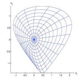
(a) $\Phi$

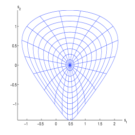
(b) $\Phi_{II}$

Figure 1: Illustrations of mappings on $\mathbb{B}^{2}$ for the region $\Omega$ given by (38)

As discussed earlier, we solve the nonlinear system (31) for a lower value of the degree $n$, usually with an initial guess associated with $u_{n}^{(0)}=0.$ As we increase $n$, we use the approximate solution from a preceding $n$ to generate an initial guess for the new value of $n$. We use the Matlab program fsolve to solve the nonlinear system. In the future we plan to look at other numerical methods that take advantage of the special structure of (31).  To estimate the error, we use as a true solution a numerical solution associated with a larger value of $n$.

For a particular case, consider the case

$$f\left(s,t,z\right)=\frac{\cos\left(\pi\,st\right)}{1+z^{2}}$$ (40)

A graph of the solution is shown in Figure 2, along with numerical results for $n=5,6,\dots,20$, with the solution $u_{25}$ taken as the true solution. We use both the mapping $\Phi$ of (38) and the mapping $\Phi_{II}$.  Using either of the mappings, $\Phi$ or $\Phi_{II}$, the graphs indicate an exponential rate of convergence for the mappings $\left\{u_{n}\right\}$. The mapping $\Phi_{II}$ is better behaved, as can be seen by visually comparing the graphs in 1. This is the probable reason for the improved convergence of the spectral method when using $\Phi_{II}$ in comparison to $\Phi$.

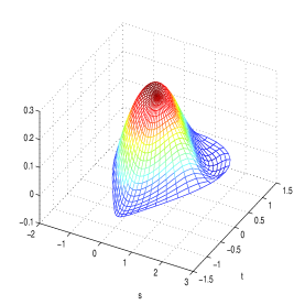
The solution $u$

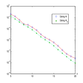
The maximum error

Figure 2: The solution u to (37) with right side (40) and its error

As a second planar example we consider the stationary Fisher equation where the function $f$ in (37) is given by

$$f(s,t,u)=100u(1-u),\quad\quad(s,t)\in\Omega.$$

Fisher’s equation is used to model the spreading of biological populations and from $f$ we see that $u=0$ and $u=1$ are stationary points for the time dependent equation on an unbounded domain; see [13, Chap. 17]. The original Fisher equation does not contain the term $100$, but for small domains the Fisher equation might have no nontrivial solution and the factor 100 corresponds to a scaling by a factor 10 to guarantee the existence of a nontrivial solution on the domain $\Omega$. The domain $\Omega$ is the interior of the curve

$$\varphi(t)=(3+\cos(t)+2\sin(t))\left(\cos t,\sin t\right)$$ (41)

We studied this domain in earlier papers (see [5]) where we called this domain a ‘Limacon domain’. In the article [5] we also describe how we use equation (41) to create a domain mapping $\Phi:\overline{\mathbb{B}}^{2}\rightarrow\overline{\Omega}$ by two dimensional interpolation. Similar to the previous example we calculate the numerical solutions $u_{n}$ for $n=1,\ldots,40$, where we use the coefficients of $u_{n-1}$ as a starting value $u_{n}^{(0)}$ for $n=2,\ldots,40$ and for $u_{1}^{(0)}$ we use coefficients which are non zero (all equal to 10), so the iteration of fsolve does not converge to the trivial solution. As a reference solution we calculated $u_{45}$; see Figure 3.

Solution for Fisher’s equation

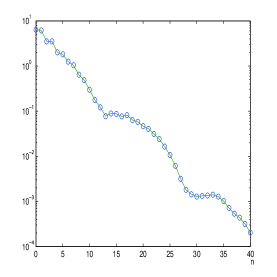
Error for Fisher’s equation

Figure 3: The reference solution and maximum error for Fisher’s equation

The shape of the solution is very much like we expect it, the function is close to $1$ inside the domain $\Omega$ and drops off very steeply to the boundary value $0$. By looking at the reference solution in Figure 3 we also see that the function will be harder to approximate by polynomials than the function in the previous example, because of the sharp drop off. This becomes clear when we look at the convergence, also shown in Figure 3. The final error is in the range of $10^{-3}$–$10^{-4}$ with a polynomial degree of 40, so the error is in the same range as in the previous example where we only used polynomials up to degree 20 for the approximation. Still the graph suggests that the convergence is exponential as predicted by (28) for the $L^{2}$ norm.

5.1 A three dimensional example

In the following we present a three dimensional example. We use the mapping $\Phi:\overline{\mathbb{B}}^{3}\rightarrow\overline{\Omega}$, $\left(s,t,v\right)=\Phi\left(x,y,z\right)$, defined by

$$\begin{array}[c]{l}s=x-y+ax^{2}\\ t=x+y\\ v=2z+bz^{2}\end{array}$$ (42)

where $a=b=0.5$. We have used this mapping in a previous article, see [2], where one finds plots of the surface $\partial\Omega$. On $\Omega$ we solve

$$-\Delta u\left(s,t,v\right)=f\left(s,t,v,u\left(s,t,v\right)\right),$$

(43)

where $f$ is defined by

$$f(s,t,v,u)=\frac{\cos(6x+y+z)}{1+u^{2}},\quad\quad(s,t,v)\in\Omega$$

We calculated approximate solutions $u_{1},\ldots,u_{20}$ and used $u_{25}$ as a reference solution. In Figure 4 we see the convergence in the maximum norm on a grid in $\overline{\mathbb{B}}^{3}$. As in our previous examples the graph suggests that we have exponential convergence.

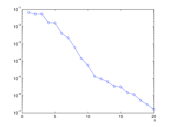
Figure 4: For the problem (43), the convergence of the  errors $\left\|u-u_{n}\right\|_{\infty}$.

In our final Figure 5 we show the graph of the reference solution $u_{25}$ on $\overline{\mathbb{B}}^{3}\cap P_{\nu}$ where $P_{\nu}$ is a plane in $\mathbb{R}^{3}$ normal to the vector $\nu$. We have used several normal vectors $\nu_{1}=(0,0,1)^{T}$, so $P_{\nu_{1}}$ is the $xy$–plane, $\nu_{2}=(0,0,1)^{T}$, so $P_{\nu_{2}}$ is the $xz$–plane, $\nu_{3}=(1,0,0)^{T}$, so $P_{\nu_{3}}$ is the $yz$–plane, and $\nu_{4}=(1,1,1)^{T}$, so $P_{\nu_{4}}$ is a diagonal plane. Figure 5 shows that the solution reflects the periodic character of the nonlinearity $f$. In the yz–plane the oscillation of $f$ is much slower which is also visible in the plot along the $yz$–plane.

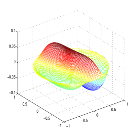
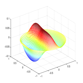
$\nu_{1}=(0,0,1),$ $P_{1}$ is $xy-plane$	$\nu_{2}=(0,1,0),$ $P_{2}$ is $xz-plane$
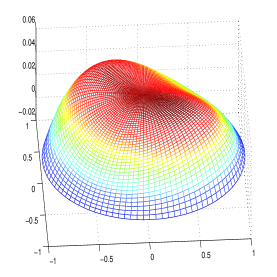
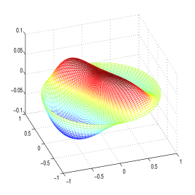
$\nu_{3}=(1,0,0),$ $P_{3}$ is $yz-plane$	$\nu_{4}=(1,1,1),$ $P_{4}$ is diagonal

Figure 5: The solution $\widetilde{u}\left(x,y,z\right)$ over $P\cap\mathbb{B}^{3}$ with $P$ a plane passing through the origin and orthogonal to $\nu$

6 Neumann boundary value problem

Consider the boundary value problem

$$-\Delta u\left(s\right)+\gamma\left(s\right)u\left(s\right)=f\left(s,u(s)\right),\quad\quad s\in\Omega,$$ (44)

$$\frac{\partial u\left(s\right)}{\partial n_{s}}=0,\quad\quad s\in\mathbb{\partial}\Omega.$$ (45)

with $n_{s}$ the exterior unit normal to $\partial\Omega$ at the boundary point $s$. Later we discuss an extension to a nonzero normal derivative over $\partial\Omega$. A necessary condition for the unknown function $u^{\ast}$ to be a solution of (44)-(45) is that it satisfy

$$\int_{\Omega}f\left(s,u^{\ast}\left(s\right)\right)\,ds=\int_{\Omega}\gamma\left(s\right)u^{\ast}\left(s\right)\,ds.$$ (46)

With our assumption that (44)-(45) has a locally unique solution $u^{\ast}$, (46) is satisfied.

Proceed in analogy with the earlier treatment of the Dirichlet problem. Use integration by parts to show that for arbitrary functions $u\in H^{2}\left(\Omega\right),$ $v\in H^{1}\left(\Omega\right)$,

$$\begin{array}[c]{r}{\displaystyle\int_{\Omega}}v(s)\left[-\Delta u(s)+\gamma(s)u\right]\,ds={\displaystyle\int_{\Omega}}\left[\triangledown u(s)\cdot\triangledown v(s)+\gamma(s)u(s)v(s)\right]\,ds\quad\vskip 6.0pt plus 2.0pt minus 2.0pt\\ -{\displaystyle\int_{\partial\Omega}}v\left(s\right)\dfrac{\partial u(s)}{\partial n_{s}}\,ds.\end{array}$$ (47)

Introduce the bilinear functional

$$\mathcal{A}\left(v_{1},v_{2}\right)=\int_{\Omega}\left[\triangledown v_{1}(s)\cdot\triangledown v_{2}(s)+\gamma(s)v_{1}(s)v_{2}(s)\right]\,ds.$$

The variational form of the Neumann problem (44)-(45) is as follows: find $u\in H^{1}\left(\Omega\right)$ such that

$$\mathcal{A}\left(u,v\right)=\left(\mathcal{F}\left(u\right),v\right),\quad\quad\forall v\in H^{1}\left(\Omega\right)$$ (48)

with, as before, the operator $\mathcal{F}$ defined by

$$\left(\mathcal{F}\left(u\right)\right)\left(s\right)=f(s,u\left(s\right)).$$

The theory for (48) is essentially the same as for the Dirichlet problem in its reformulation (6).

Because of changes that take place in the normal derivative under the transformation $s=\Phi\left(x\right)$, we modify the construction of the numerical method. In the actual implementation, however, it will mirror that for the Dirichlet problem. For the approximating space, let

$$\mathcal{X}_{n}=\left\{q\mid q\circ\Phi=p\text{ for some }p\in\Pi_{n}^{d}\right\}.$$

For the numerical method, we seek $u_{n}^{\ast}\in\mathcal{X}_{n}$ for which

$$\mathcal{A}\left(u_{n}^{\ast},v\right)=\left(\mathcal{F}\left(u_{n}^{\ast}\right),v\right),\quad\quad\forall v\in\mathcal{X}_{n}.$$ (49)

A similar approach was used in [6] for the linear Neumann problem.

To carry out a convergence analysis for (49), it is necessary to compare convergence of approximants in $\mathcal{X}_{n}$ to that of approximants from $\Pi_{n}^{d}.$ For simplicity in notation, we assume $\Phi\in C^{\infty}\left(\overline{\mathbb{B}}^{d}\right)$. Begin by referring to Lemma 1 and its discussion in §2.1, linking differentiability in $H^{m}\left(\Omega\right)$ and $H^{m}\left(\mathbb{B}^{d}\right)$. In particular, for $m\geq 0$,

$$c_{1,m}\left\|v\right\|_{H^{m}\left(\Omega\right)}\leq\left\|\widetilde{v}\right\|_{H^{m}\left(\mathbb{B}^{d}\right)}\leq c_{2,m}\left\|v\right\|_{H^{m}\left(\Omega\right)},\quad\quad v\in H^{m}\left(\Omega\right),$$ (50)

with $\widetilde{v}=v\circ\Phi$, with constants $c_{1,m},c_{2,m}>0$.

Also recall Theorem 2 concerning approximation of functions $\widetilde{v}\in H^{r}\left(\mathbb{B}^{d}\right)$ and link this to approximation of functions $v\in H^{r}\left(\Omega\right)$.

Lemma 7

Assume $\Phi\in C^{\infty}\left(\overline{\mathbb{B}}^{d}\right)$. Assume $v\in H^{r}\left(\Omega\right)$ for some $r\geq 2$. Then there exist a sequence $q_{n}\in\mathcal{X}_{n}$, $n\geq 1$, for which

$$\left\|v-q_{n}\right\|_{H^{1}\left(\Omega\right)}\leq\varepsilon_{n,r}\left\|v\right\|_{H^{r}\left(\Omega\right)},\quad\quad n\geq 1.$$ (51)

The sequence $\varepsilon_{n,r}=\mathcal{O}\left(n^{-r+1}\right)$ and is independent of $v$.

Proof. Begin by applying Theorem 2 to the function $\widetilde{v}\left(x\right)=v\left(\Phi\left(x\right)\right)$. Then there is a sequence of polynomials $p_{n}\in\Pi_{n}^{d}$ for which

$$\left\|\widetilde{v}-p_{n}\right\|_{H^{1}\left(\mathbb{B}^{d}\right)}\leq\varepsilon_{n,r}\left\|\widetilde{v}\right\|_{H^{r}\left(\mathbb{B}^{d}\right)},\quad\quad n\geq 1.$$

Let $q_{n}=p_{n}\circ\Phi^{-1}$. The result then follows by applying (50).   

The theoretical convergence analysis now follows exactly that given earlier for the Dirichlet problem. Again we use the construction from [19, §4(a)], but now use the integral operator $\mathcal{T}$ arising from the zero Neumann boundary condition. As with the Dirichlet problem, it is necessary to have $\mathcal{A}$ be strongly elliptic, and for that reason and without any loss of generality, assume

$$\min_{s\in\overline{\Omega}}\gamma\left(s\right)>0.$$

The solution of (48) can be written as $u=\mathcal{TF}\left(u\right)$ with $\mathcal{T}:L_{2}\left(\mathbb{B}^{d}\right)\rightarrow H^{2}\left(\mathbb{B}^{d}\right)$ and bounded. Use Theorem 2 in place of Theorem 3 for polynomial approximation error, as in the derivation of (26).  Theorems 4 and 5, along with Corollary 6 are valid for the spectral method for the Neumann problem (44)-(45).

6.1 Implementation

As in §4, we look for a solution to (48) by looking for

$$u_{n}\left(s\right)=\sum_{\ell=1}^{N_{n}}\alpha_{\ell}\psi_{\ell}\left(s\right)$$ (52)

with  $\left\{\psi_{\ell}:1\leq j\leq N_{n}\right\}$ a basis for $\mathcal{X}_{n}$. The system associated with (48) that is to be solved is

$$\begin{array}[c]{l}{\displaystyle\sum\limits_{\ell=1}^{N_{n}}}\alpha_{\ell}{\displaystyle\int_{\Omega}}\left[{\displaystyle\sum\limits_{i,j=1}^{d}}a_{i,j}(s)\dfrac{\partial\psi_{\ell}(s)}{\partial s_{i}}\dfrac{\partial\psi_{k}(s)}{\partial s_{j}}+\gamma\left(s\right)\psi_{\ell}\left(s\right)\psi_{k}\left(s\right)\right]\,ds\quad\vskip 3.0pt plus 1.0pt minus 1.0pt\\ \quad\quad={\displaystyle\int_{\Omega}}f\left(s,{\displaystyle\sum\limits_{\ell=1}^{N_{n}}}\alpha_{\ell}\psi_{\ell}\left(s\right)\right)\psi_{k}(s)\,ds,\quad\quad k=1,\dots,N_{n}.\end{array}$$ (53)

For such a basis $\left\{\psi_{\ell}\right\}$, we begin with an orthonormal basis for $\Pi_{n}$, say $\{\varphi_{j}:1\leq j\leq N_{n}\}$, and then define

$$\psi_{\ell}\left(s\right)=\varphi_{\ell}\left(x\right)\quad\text{\emph{with\quad}}s=\Phi\left(x\right),\quad\quad 1\leq\ell\leq N.$$

The function $\widetilde{u}_{n}\left(x\right)\equiv u_{n}\left(\Phi\left(x\right)\right)$, $x\in\mathbb{B}^{d},$ is to be the equivalent solution considered over $\mathbb{B}^{d}.$ Using the transformation of variables $s=\Phi\left(x\right)$ in the system (53), the coefficients $\left\{\alpha_{\ell}|\ell=1,2,\dots,N_{n}\right\}$ are the solutions of

$$\begin{array}[c]{r}{\displaystyle\sum\limits_{k=1}^{N_{n}}}\alpha_{k}{\displaystyle\int_{\mathbb{B}^{d}}}\left[{\displaystyle\sum\limits_{i,j=1}^{d}}\widetilde{a}_{i,j}(x)\dfrac{\partial\varphi_{k}(x)}{\partial x_{j}}\dfrac{\partial\varphi_{\ell}(x)}{\partial x_{i}}+\gamma(\Phi\left(x\right))\varphi_{k}(x)\varphi_{\ell}(x)\right]\det J\left(x\right)\,dx\vskip 6.0pt plus 2.0pt minus 2.0pt\\ ={\displaystyle\int_{\mathbb{B}^{d}}}f\left(x,{\displaystyle\sum\limits_{k=1}^{N_{n}}}\alpha_{k}\varphi_{k}\left(x\right)\right)\varphi_{\ell}\left(x\right)\det J\left(x\right)\,dx,\quad\quad\ell=1,\dots,N_{n}\end{array}$$ (54)

For the equation (44) the matrix $A\left(s\right)$ is the identity, and therefore from (19),

$$\widetilde{A}\left(x\right)=J\left(x\right)^{-1}J\left(x\right)^{-\text{T}}.$$

The system (54) is much the same as (31) for the Dirichlet problem, differing only by the basis functions being used for the solution $\widetilde{u}_{n}$. We use the same numerical integration as before, and also the same orthonormal basis for $\Pi_{n}^{d}$.

6.2 Numerical example

Consider the problem

$$-\Delta u\left(s,t\right)+u\left(s,t\right)=f\left(s,t,u\left(s,t\right)\right),$$

(55)

with $\Omega$ the elliptical region

$$\left(\frac{s}{a}\right)^{2}+\left(\frac{t}{b}\right)^{2}\leq 1.$$

The mapping of $\mathbb{B}^{2}$ onto $\Omega$ is simply

$$\Phi\left(x,y\right)=\left(ax,by\right),\quad\quad\left(x,y\right)\in\overline{\mathbb{B}}^{2}.$$

As before, note the change in notation, from $s\in\mathbb{R}^{2}$ to $\left(s,t\right)\in\mathbb{R}^{2}$.

The right side $f$ is given by

$$f\left(s,t,u\right)=-e^{u}+f_{1}\left(s,t\right)$$ (56)

with the function $f_{1}$ determined from the given true solution and the equation (55) to define $f\left(s,t,u\right)$. In our case,

$$u\left(s,t\right)=\left(1-\left(\frac{s}{a}\right)^{2}-\left(\frac{t}{b}\right)^{2}\right)^{2}\cos\left(2s+t^{2}\right).$$ (57)

Easily this has a normal derivative of zero over the boundary of $\Omega$.

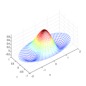
Solution (57)

Maximum error

Figure 6: The solution u to (55) with right side (56) and true solution (57)

The nonlinear system (54) was solved using fsolve from Matlab, as earlier in §5. Our region $\Omega$ uses $\left(a,b\right)=\left(2,1\right)$. Figure 6 contains the approximate solution for $n=18$ and also shows the maximum error over $\overline{\Omega}$. Again, the convergence appears to be exponential.

6.3 Handling a nonzero Neumann condition

Consider the problem

$$-\Delta u\left(s\right)+\gamma\left(s\right)u\left(s\right)=f\left(s,u(s)\right),\quad\quad s\in\Omega,$$ (58)

$$\frac{\partial u\left(s\right)}{\partial n_{s}}=g(s),\quad\quad s\in\mathbb{\partial}\Omega$$ (59)

with a nonzero Neumann boundary condition. Let $u^{\ast}\left(s\right)$ denote the solution we are seeking. A necessary condition for solvability of (58)-(59) is that

$$\int_{\Omega}f\left(s,u^{\ast}\left(s\right)\right)\,ds=\int_{\Omega}\gamma\left(s\right)u^{\ast}\left(s\right)\,ds-\int_{\partial\Omega}g\left(s\right)\,ds.$$ (60)

There are at least two approaches to extending our spectral method to solve this problem.

First, consider the problem

$$-\Delta v\left(s\right)=c_{0},\quad\quad s\in\Omega,$$ (61)

$$\frac{\partial v\left(s\right)}{\partial n_{s}}=g(s),\quad\quad s\in\mathbb{\partial}\Omega,$$ (62)

with $c_{0}$ a constant. From (60), solvability of (61)-(62) requires

$$\int_{\Omega}c_{0}\,ds=-\int_{\partial\Omega}g\left(s\right)\,ds,$$ (63)

is satisfied. To do so, choose

$$c_{0}=\frac{-1}{\operatorname*{Vol}\left(\Omega\right)}\int_{\partial\Omega}g\left(s\right)\,ds.$$

A solution $v^{\ast}\left(s\right)$ exists, although it is not unique. The solution of (61)-(62) can be approximated using the method given in [6]. Then introduce

$$w=u-v^{\ast}.$$

Substituting into (58)-(59), the new unknown function $w^{\ast}$ satisfies

$$-\Delta w\left(s\right)+\gamma\left(s\right)w\left(s\right)=f\left(s,w(s)+v^{\ast}\left(s\right)\right)-\gamma\left(s\right)v^{\ast}\left(s\right)-c_{0},\quad\quad s\in\Omega,$$ (64)

$$\frac{\partial w\left(s\right)}{\partial n_{s}}=0,\quad\quad s\in\mathbb{\partial}\Omega.$$ (65)

The methods of this section can be used to approximate $w^{\ast}$; and then use $u^{\ast}=w^{\ast}+v^{\ast}.$

A second approach is to use (47) to reformulate (58)-(59) as the problem of finding $u=u^{\ast}$ for which

$$\mathcal{A}\left(u,v\right)=\left(\mathcal{F}\left(u\right),v\right)+\ell\left(v\right),\quad\quad\forall v\in H^{1}\left(\Omega\right)$$ (66)

with

$$\ell\left(v\right)=\int_{\partial\Omega}v\left(s\right)g\left(s\right)\,ds.$$

Thus we seek

$$u_{n}\left(s\right)=\sum_{\ell=1}^{N_{n}}\alpha_{\ell}\psi_{\ell}\left(s\right)$$

for which

$$\mathcal{A}\left(u_{n},v\right)=\left(\mathcal{F}\left(u\right),v\right)+\ell\left(v\right),\quad\quad\forall v\in\mathcal{X}_{n}.$$ (67)

The first approach, that of (58)-(65), is usable, and the convergence analysis follows from combining this paper’s analysis with that of [6]. Unfortunately, we do not have a convergence analysis  for this second approach, that of (66)-(67), as the Green’s function approach of this paper does not seem to extend to it.

References

[1]K. Atkinson. The numerical evaluation of fixed points for
completely continuous operators, SIAM J. Num. Anal.10 (1973),
pp. 799-807.
[2]K. Atkinson, D. Chien, and O. Hansen. A spectral method for
elliptic equations: The Dirichlet problem, Advances in Computational
Mathematics, 33 (2010), pp. 169-189.
[3]K. Atkinson, D. Chien, and O. Hansen. Evaluating polynomials
over the unit disk and the unit ball, Numerical Algorithms67
(2014), pp. 691-711.
[4]K. Atkinson and O. Hansen. A spectral method for the
eigenvalue problem for elliptic equations, Electronic Transactions on
Numerical Analysis37 (2010), pp. 386-412.
[5]K. Atkinson and O. Hansen. Creating domain mappings,
Electronic Transactions on Numerical Analysis39 (2012), pp. 202-230.
[6]K. Atkinson, O. Hansen, and D. Chien. A spectral method for
elliptic equations: The Neumann problem, Advances in Computational
Mathematics34 (2011), pp. 295-317.
[7]K. Atkinson,O. Hansen, and D. Chien. A spectral method for
parabolic differential equations, Numerical Algorithms63
(2013), pp. 213-237.
[8]K. Atkinson and W. Han. Theoretical Numerical
Analysis: A Functional Analysis Framework, 3 ed.,
Springer-Verlag, 2009.
[9]K. Atkinson and W. Han. An Introduction to Spherical
Harmonics and Approximations on the Unit Sphere, Springer-Verlag, 2012
[10]F. Dai and Y. Xu. Approximation Theory and Harmonic
Analysis on Spheres and Balls, Springer-Verlag, 2013.
[11]C. Dunkl and Y. Xu. Orthogonal Polynomials of Several
Variables, Cambridge Univ. Press, 2001.
[12]W. Gautschi. Orthogonal Polynomials, Oxford
University Press, 2004.
[13]Mark Kot. Elements of Mathematical Ecology, Cambridge
University Press, 2001.
[14]Huiyuan Li and Yuan Xu. Spectral approximation on the the unit
ball, SIAM J. Num. Anal.52 (2014), pp. 2647-2675.
[15]B. Logan and L. Shepp. Optimal reconstruction of a function
from its projections, Duke Mathematical Journal42, (1975), 645–659.
[16]M. Krasnoseľskii. Topological Methods in the
Theory of Nonlinear Integral Equations, Pergamon Press, 1964.
[17]T. M. MacRobert, Spherical Harmonics, Dover
Publications, Inc., 1948.
[18]F. Olver, D. Lozier, R. Boisvert, and C. Clark (Editors).
NIST Handbook of Mathematical Functions, Cambridge University Press, 2010.
[19]John Osborn. Spectral approximation for compact
operators, Mathematics of Computation29 (1975), pp. 712-725.
[20]A. Stroud. Approximate Calculation of Multiple
Integrals, Prentice-Hall, Inc., 1971.
[21]Yuan Xu. Lecture notes on orthogonal polynomials of several
variables, in Advances in the Theory of Special Functions and Orthogonal
Polynomials, Nova Science Publishers, 2004, 135-188.
[22]E. Zeidler. Nonlinear Functional Analysis and Its
Applications: II/B, Springer-Verlag, 1990.
(a)
(a)
(b)
(b)