Molecular dynamics study of the stability of a carbon nanotube atop a catalytic nanoparticle

Abstract

The stability of a single-walled carbon nanotube placed on top of a catalytic nickel nanoparticle is investigated by means of molecular dynamics simulations. As a case study, we consider the $(12,0)$ nanotube consisting of 720 carbon atoms and the icosahedral Ni₃₀₉ cluster. An explicit set of constant-temperature simulations is performed in order to cover a broad temperature range from 400 to 1200 K, at which a successful growth of carbon nanotubes has been achieved experimentally by means of chemical vapor deposition. The stability of the system depending on parameters of the involved interatomic interactions is analyzed. It is demonstrated that different scenarios of the nanotube dynamics atop the nanoparticle are possible depending on the parameters of the Ni–C potential. When the interaction is weak the nanotube is stable and resembles its highly symmetric structure, while an increase of the interaction energy leads to the abrupt collapse of the nanotube in the initial stage of simulation. In order to validate the parameters of the Ni–C interaction utilized in the simulations, DFT calculations of the potential energy surface for carbon-nickel compounds are performed. The calculated dissociation energy of the Ni–C bond is in good agreement with the values, which correspond to the case of a stable and not deformed nanotube simulated within the MD approach.

1 Introduction

During past decades, mass production synthesis of carbon nanotubes Iijima_1991_Nature.354.56 has been achieved by various methods such as arc discharge Journet_1997_Nature.388.756 , laser ablation Smalley_1996_Science.273.483 , and pyrolysis Terrones_1997_Nature.388.52 . In these methods, the growth of nanotubes is initiated by condensation of a hot carbon-rich gas. These approaches does not allow for an easy control of the diameter, length and chirality of nanotubes that strongly affect physical and mechanical properties of the systems Choi_2000_ApplPhysLett.76.2367 . Thus, different variations of the chemical vapor deposition (CVD) method have been utilized in order to synthesize nanotubes of higher purity and with more selective growth parameters Choi_2000_ApplPhysLett.76.2367 ; Li_2008_MaterLett.62.1472 ; Yuan_2008_NanoLett.8.2576 ; Kang_2009_JMaterSci.44.2471 ; Diao_2010_AdvMater.22.1430 . In this method, the nanotube growth is determined by the presence of a catalytic nanoparticle (usually made of transition elements like Ni, Co and Fe), which causes the separation of carbon present in the precursor gas (e.g., CO, C₂H₂, or CH₄) and then assists as seed-site for the growth Martinez-Limia_2007_JMolModel.13.595 .

It has been found that the structure of carbon nanotubes is dependent on synthesis parameters such as the reaction temperature Li_2008_MaterLett.62.1472 , the composition and size of a catalytic particle Choi_2000_ApplPhysLett.76.2367 ; Yuan_2008_NanoLett.8.2576 ; Harris_2007_Carbon.45.229 ; Kang_2008_MaterSciEngA.475.136 , the reaction gas Harris_2007_Carbon.45.229 ; SaitoBook , etc. In spite of an intense study of the growth mechanism of carbon nanotubes, its details are not yet fully understood, so the current synthesis methods do not allow for a full control of the growth Harutyunyan_2005_ApplPhysLett.87.051919 . In particular, there has been much discussion during past years on the phase of catalysts in the course of the nanotube synthesis Harutyunyan_2005_ApplPhysLett.87.051919 ; Kanzow_1999_PhysRevB.60.11180 ; Gavillet_2001_PhysRevLett.87.275504 ; Ding_2004_JChemPhys.121.2775 . Typically, the process of the nanotube growth by CVD methods is conducted at elevated temperatures approximately ranging from 900 to 1500 K Harutyunyan_2005_ApplPhysLett.87.051919 ; Cui_2000_JApplPhys.88.6072 ; Jeong_2003_JpnJApplPhys.42.L1340 . Although these values are significantly lower than the melting temperature of bulk metals that typically comprise the catalyst, the nanoparticles can be in the molten state due to the well-established dependence of the melting temperature of small nanoparticles on their radius, $T_{m}=T_{m}^{\rm bulk}\left(1-\alpha/R\right)$, where $T_{m}^{\rm bulk}$ is the bulk melting temperature, $R$ is the radius of a spherical nanoparticle and $\alpha$ is the factor of proportionality Pawlow_1909_ZPhysChem.65 ; Qi_2001_JChemPhys.115.385 ; Lyalin_2009_PhysRevB.79.165403 ; Yakubovich_2013_PhysRevB.88.035438 . In Ref. Harutyunyan_2005_ApplPhysLett.87.051919 it was found that the liquid phase of an iron catalytic nanoparticle is favored for the growth of nanotubes, while the solidification of the catalyst nearly terminates the growth. On the other hand, a number of successful attempts to lower the nanotube synthesis temperature by the plasma-enhanced CVD method have been reported Hofmann_2003_ApplPhysLett.83.135 ; Shang_2010_Nanotech.21.505604 ; He_2011_NanoRes.4.334 ; Halonen_2011_PhysStatSolb.248.2500 . In particular, this method has allowed one to grow vertically aligned nanotubes at temperatures as low as 400 K with nickel as a catalyst Hofmann_2003_ApplPhysLett.83.135 . In the case of such a low-temperature growth, the catalytic nanoparticle certainly remains in the solid state.

In spite of intensive research and a huge amount of collected experimental information, the physical mechanisms leading to the catalytically-assisted carbon nanotube growth remain a highly debated issue. A limited understanding of the detailed growth mechanism hinders further progress in the carbon nanotube production such as the selective growth of nanotubes having a specific diameter and/or chirality Diao_2010_AdvMater.22.1430 ; Harris_2007_Carbon.45.229 .

Numerical studies based on molecular dynamics (MD) simulations have provided deeper understanding of the catalyzed nanotube growth and its initial stage, in particular, on the atomistic level Ding_2004_JChemPhys.121.2775 ; Irle_2009_NanoRes.2.755 ; Ohta_2009_Carbon.47.1270 ; Shibuta_2003_ChemPhysLett.382.381 ; Zhao_2005_Nanotechnology.16.S575 . The performed simulations have illustrated the diffusion of carbon atoms into the catalytic nanoparticle that is followed by the cap formation process when the concentration of carbon atoms in the catalyst exceeds some critical value. Classical MD simulations, based on the so-called reactive empirical bond-order (REBO) potential Tersoff88 ; Brenner90 , of the nanotube growth on a metal catalyst have shown that the following three stages of the process can be distinguished Ding_2004_JChemPhys.121.2775 ; Shibuta_2003_ChemPhysLett.382.381 . At first, carbon atoms dissolve in the metal nanoparticle, then a small graphitic island starts to nucleate on the cluster surface. Finally, the metal nanoparticle becomes covered by carbon atoms and, depending on temperature, a graphite sheet or a carbon nanotube is formed. However, the resulting structure of modeled nanotubes contained a significant number of defects, such as four-, five-, seven- or eight-membered rings, that made the prediction of the nanotube chirality hardly possible.

In the meantime, Smalley and co-workers have reported Smalley_2006_JACS.128.15824 on the successful experimental attachment of a short single-walled nanotube to iron nanoparticles and showed that continued growth of the nanotube can be achieved. During the last years, several theoretical studies of the continued growth of a single-walled carbon nanotube on small iron clusters were performed using quantum MD simulations Irle_2009_NanoRes.2.755 ; Ohta_2008_ACSNano.2.1437 . In these studies, it was shown that due to the random nature of new polygon formation, the tube sidewall growth is observed as an irregular process without clear nanotube chirality.

In Ref. Solovyov_2008_PhysRevE.78.051601 the so-called liquid surface model for calculating the energy of single-walled carbon nanotubes with arbitrary chirality was introduced. The model allowed one to predict the energy of a nanotube once its chirality and the total number of atoms are known. The suggested model gave an insight in the energetics and stability of nanotubes of different chirality and was considered as an important tool for the understanding of the nanotube growth.

In spite of an intensive experimental and theoretical research carried out within the past few decades, details of the carbon nanotube stabilization mechanism on metal nanoparticles are not yet completely understood, although they can strongly affect the continued growth scenario. In the present study, we investigate the process of the carbon nanotube stabilization on a catalytic nickel nanoparticle by means of classical MD simulations. In particular, we analyze how the reaction temperature affects the nanotube stability. For this purpose, we have performed a set of constant-temperature simulations, which cover the whole range of temperatures currently achieved in CVD and PECVD methods. A very important problem of the numerical method, based on MD simulations, is a proper choice of interatomic potentials and their parameters. Thus, we consider a broad range of parameters for the nanotube-catalyst interaction and demonstrate that, depending on the parameters of a Ni–C interatomic potential, different scenarios of the nanotube dynamics atop the nanoparticle are possible. In order to validate the parameters of the Ni–C interaction, utilized in the simulations, we perform a set of ab initio calculations of the potential energy surface for two Ni–C-based compounds, namely for a Ni atom linked to a benzene molecule and to a small carbon chain. Considering these case studies, we have accounted for different types of Ni–C interaction, that exist when nickel atoms interact either with the nanotube sidewall or with its open end. The resulting dissociation energy of the Ni–C bond is in good agreement with the values, which are utilized in MD simulations describing the stable system.

2 Theoretical framework

2.1 Description of the system

In this study, we analyze the stability of a single-walled carbon nanotube placed atop a nickel nanoparticle by means of MD simulations. As a case study, we consider a 6.24 nm-long uncapped nanotube of the $(12,0)$ chirality consisting of 720 carbon atoms. The diameter of the nanotube is equal to 0.94 nm. In its initial configuration, the nanotube is aligned along the $z$ axis, as illustrated in Figure 1(a). The geometrical structure of the nanotube was obtained using the Nanotube Builder tool of the VMD program VMD_reference , which was also used for the visualization of the results. The nanotube is positioned over the top face of the icosahedral Ni₃₀₉ cluster, which has a radius of approximately 1.8 nm. The initial structure of the system under study is presented in Figure 1(a).

In order to investigate the nanotube dynamics on top of the catalytic nickel nanoparticle, we have conducted an explicit set of constant-temperature MD simulations. They were performed using MBN Explorer MBN_Explorer1 ; MBN_Explorer2 , a universal software package for multiscale simulation of complex molecular structure and dynamics. During past years it has been utilized for structure optimization Solovyov_2003_PhysRevLett.90.053401 ; Geng_2010_PhysRevB.81.214114 , simulation of dynamics Yakubovich_2013_PhysRevB.88.035438 ; Verkhovtsev_2013_ComputMaterSci.76.20 ; Yakubovich_2013_ComputMaterSci.76.60 ; Sushko_2013_JCompPhys.252.404 and growth processes Dick_2011_PhysRevB.84.115408 ; Solovyov_2013_PhysStatSolB ; Panshenskov_3d-KMC in various molecular and bio/nanosystems. Integration of equations of motion was done using the Verlet leap frog algorithm with a time step of 1 fs and a total simulation time of 5 ns. The total energy of the system and coordinates of all atoms were recorded each 1 ps of the simulation. The temperature control was achieved by means of the Langevin thermostat with a damping constant $\gamma=0.1$ ps^-1. In this case, the dynamics of atoms in the system is described by Langevin equations of motion:

$$m_{i}{\bf a}_{i}(t)={\bf F}_{i}(t)-\frac{1}{\tau_{d}}m_{i}{\bf v}_{i}(t)+\sqrt{\frac{2k_{B}T_{0}m_{i}}{\tau_{d}}}\,{\bf R}_{i}(t)\ ,$$ (1)

where ${\bf F}_{i}$ is the physical force acting on the atom, $k_{B}T$ denotes the thermal energy in the system, $\tau_{d}\equiv 1/\gamma$ is the characteristic viscous damping time, and ${\bf R}_{i}(t)$ represents random forces, which act on the particle as a result of solvent interaction. The Langevin equation of motion gives a physically correct description of a many-particle system interacting with a heat bath maintained at a constant temperature $T_{0}$ MBN_Explorer1 .

Calculations performed within the classical framework were carried out using empirical interatomic potentials. The total potential energy of the system is defined as follows:

$$U=U^{\rm Ni-Ni}+U^{\rm C-C}+U^{\rm Ni-C}\ ,$$ (2)

where the terms $U^{\rm Ni-Ni}$, $U^{\rm C-C}$ and $U^{\rm Ni-C}$ refer to the nickel-nickel, carbon-carbon and nickel-carbon interaction, respectively. A detailed description of the potentials used in the calculations is given in the following subsections.

2.2 Nickel-nickel interaction

The interaction between nickel atoms is described in the present study using the many-body Finnis-Sinclair-type potential Finnis-Sinclair . Recently, this interatomic potential has been successfully utilized for studying the diffusion process in both ideal and nanostructured titanium and nickel-titanium crystalline samples Yakubovich_2013_ComputMaterSci.76.60 ; Sushko_2014_JPhysChemA2 , as well as for analysis of mechanical properties of these materials by means of MD simulations of nanoindentation Verkhovtsev_2013_ComputMaterSci.76.20 ; Verkhovtsev_2013_ComputTheorChem.1021.101 ; Sushko_2014_JPhysChemA .

The general structure of many-body potentials Finnis-Sinclair ; Gupta ; Sutton_Chen ; Daw_1993_MaterSciRep.9.251 ; Rafii-Tabar_potentials ; TB-SMA contains an attractive density-dependent many-body term and a repulsive part for small distances that results from the repulsion between core electrons of neighboring atoms.

In the Finnis-Sinclair representation, the total energy of an $N$-atom system is written as:

$$U_{\rm FS}=\frac{1}{2}\sum_{i=1}^{N}\sum_{j\neq i}V(r_{ij})-c\sum_{i}\sqrt{\rho_{i}}\ ,$$ (3)

where

$$\rho_{i}=\sum_{j\neq i}\phi(r_{ij})\ .$$ (4)

Here the function $V(r_{ij})$ is a pairwise repulsive interaction between atoms $i$ and $j$ separated by a distance $r_{ij}$, the function $\phi(r_{ij})$ describes an attractive pair potential, and $c$ is a positive constant. The second term in Eq. (3) represents the attractive many-body contribution to the total energy of the system. The square root form of this term is chosen in the FS approach in order to mimic the result of tight-binding theory, in which $\phi(r)$ is interpreted as a sum of squares of overlap integrals Finnis-Sinclair . According to this approach (see, e.g., Rafii-Tabar_potentials ; TB-SMA ; TB-SMA_2 and references therein), the energy of the $d$ electron band in metals

$$E_{\rm band}=\sum_{i}E_{i}=2\sum_{i}\int\limits_{-\infty}^{E_{F}}E\,n_{i}(E)\,{\rm d}E$$ (5)

is proportional to the square root of the second moment of the density of states. Here $E_{i}$ is the contribution to the total electronic band energy from an individual atom $i$, $n_{i}(E)$ the density of states projected on site $i$, $E_{F}$ the Fermi level energy, and prefactor 2 in Eq. (5) arises due to spin degeneracy Rafii-Tabar_potentials . The second moment $\mu_{2}^{i}$ of the density of states, defined as

$$\mu_{2}^{i}=\int\limits_{-\infty}^{+\infty}E^{2}\,n_{i}(E)\,{\rm d}E\ ,$$ (6)

provides a measure of the squared band width and allows one to derive an approximate expression for the band energy in terms of $\mu_{2}^{i}$. This function can also be expressed as

$$\mu_{2}^{i}=\sum_{j}h_{ij}^{2}\ ,$$ (7)

where

$$h_{ij}=\langle\chi_{i}\,|\,H\,|\,\chi_{j}\rangle\ ,$$ (8)

$\chi_{i}$ is the localized orbital centered on atom $i$, and $H$ the single-electron Hamiltonian. The electron band energy $E_{i}$ is then expressed as

$$E_{i}\equiv E_{i}(\mu_{2}^{i})=-A\sqrt{(\mu_{2}^{i})}=-A\sqrt{\sum_{j}h_{ij}^{2}}\ ,$$ (9)

where $A$ is a positive constant that depends on the chosen density of states shape (see Ref. Rafii-Tabar_potentials and references therein). The square root form of this term is chosen since $E_{i}$ has units of energy and $\mu_{i}^{2}$ has units of energy squared.

The functions $\phi(r_{ij})$ in Eq. (4) can thus be interpreted as the sum of squares of overlap integrals Rafii-Tabar_potentials ; Li_2007_JPhysCondMatter.19.086228 . The function $\rho_{i}$ in the FS approach can be interpreted as a measure of the local density of atomic sites Finnis-Sinclair . Note that the Finnis-Sinclair potential, Eq. (3), is similar in form to the embedded-atom model (EAM) potential Daw_1993_MaterSciRep.9.251 , although the interpretation of the function $\rho_{i}$ is different in the two cases. In the EAM approach, $\rho_{i}$ stands for the local electronic charge density at site $i$ constructed by a rigid superposition of atomic charge densities $\phi(r_{ij})$. In other words, $\rho_{i}$ is the host electron density induced at site $i$ by all other atoms. In this case, the energy of an atom at site $i$ is assumed to be identical to its energy within a uniform electron gas of that density Daw_1983_PhysRevLett.50.1285 ; Daw_1984_PhysRevB.29.6443 .

Similar to the original second-moment approximation of the tight-binding (TB-SMA) scheme, the functions $V(r_{ij})$ and $\phi(r_{ij})$ in Eq. (3) and (4) are introduced in exponential forms TB-SMA ; TB-SMA_2 . As indicated in Ref. TB-SMA , the standard dependence of the band energy on radial interatomic distance between atoms $i$ and $j$ should rather be proportional to $r^{-4}$ or $r^{-5}$, although an exponential form of this dependence better accounts for atomic relaxation near impurities and surfaces Tomanek_1985_PhysRevB.32.5051 .

Finally, the total potential energy, $U\equiv U^{\rm Ni-Ni}$, of a system of $N$ nickel atoms, located at positions ${\bf r}_{i}$, in the Finnis-Sinclair representation reads as:

$$U=\sum_{i=1}^{N}\left[\sum_{\begin{subarray}{c}j=1\\ (i\neq j)\end{subarray}}^{N}A\,{\rm e}^{-p\left(\frac{r_{ij}}{d}-1\right)}\right.-\left.\sqrt{\sum_{\begin{subarray}{c}j=1\\ (i\neq j)\end{subarray}}^{N}\xi^{2}\,{\rm e}^{-2q\left(\frac{r_{ij}}{d}-1\right)}}\,\right]\ ,$$ (10)

where $r_{ij}$ is the distance between atoms $i$ and $j$, and $d$, $p$, $q$, $A$ and $\xi$ are adjustable parameters of the potential. The parameter $d$ is the first-neighbor distance, $\xi$ results from an effective hopping integral, $q$ describes its dependence on the relative interatomic distance, and the parameter $p$ is related to the compressibility of the bulk metal TB-SMA .

Note that the Finnis-Sinclair-type potential, as implemented in MBN Explorer MBN_Explorer1 ; MBN_Explorer2 , can be applied not only for monoatomic systems, but also for bimetallic compounds Verkhovtsev_2013_ComputTheorChem.1021.101 ; Sushko_2014_JPhysChemA . In the latter case, the aforementioned parameters, $d\equiv d_{\alpha\beta}$, etc., depend on the type of an atom, $\alpha/\beta$, chosen within the summation. When $\alpha=\beta$, as in the present study where only the Ni–Ni interaction is described, such a type of the potential is also referred to in the literature as the Gupta potential Gupta .

In order to describe the interaction between nickel atoms, we used the parametrization introduced in Ref. Lai_2000_JPhysCondMatter.12.L53 that reproduces main mechanical and structural properties of bulk nickel crystal at zero temperature. The parameters provided for nickel have the following values: $d=2.49$ Å, $A=0.104$ eV, $p=11.198$, $\xi=1.591$ eV, and $q=2.413$ Lai_2000_JPhysCondMatter.12.L53 .

Since most of the many-body potentials approach zero at large distances, a cutoff radius $r_{c}$ is frequently introduced to reduce the computation time. In this case, the interatomic potentials and, subsequently, the forces are neglected for atoms positioned at distances larger than $r_{c}$ from each other. The utilized parameter set Lai_2000_JPhysCondMatter.12.L53 was constructed with a fixed cutoff radius of 4.2 Å. In order to avoid the effect of non-continuity of the potential due to its non-zero value at the cutoff radius, we have implemented a polynomial switching from the original potential value at the cutoff radius of 4.2 Å, to zero value at the extended cutoff radius of 5.5 Å. Coefficients of the splines were determined to correspond to the value and the first derivative of the potential at the initial cutoff and to be equal to zero at 5.5 Å Verkhovtsev_2013_ComputTheorChem.1021.101 .

2.3 Carbon-carbon interaction

In order to describe the carbon-carbon interaction, we employed the Brenner empirical potential Brenner90 , which was developed for studying carbon-based systems with different types of covalent bonds. It is a REBO-type potential, which is able to account for the bond breaking/formation using a distance-dependent many-body order term and correctly dissociating diatomic potentials Irle_2009_NanoRes.2.755 .

For every atom in the system, this many-body potential depends on the nearest neighbors of this atom. The total energy, $U^{\rm C-C}$, of the system of $N$ carbon atoms interacting via the Brenner potential is expressed as a sum of bonding energies between all atoms:

$$U^{\rm C-C} = \frac{1}{2}\sum_{i=1}^{N}\sum_{\begin{subarray}{c}j=1\\ (i\neq j)\end{subarray}}^{N}U_{ij}$$

$$= \frac{1}{2}\sum_{i}\sum_{j\neq i}f_{\rm cut}(r_{ij})\left[U^{\rm(R)}(r_{ij})-B_{ij}U^{\rm(A)}(r_{ij})\right]\ ,$$

where $f_{\rm cut}(r_{ij})$ is the cutoff function, which limits the interaction of an atom to its nearest neighbors:

$$f_{\rm cut}(r_{ij})=\left\{\begin{array}[]{ll}1&,\ r_{ij}\leq R_{1}\\ \displaystyle{\frac{1}{2}}\left[1+\cos{\displaystyle{\left(\frac{r_{ij}-R_{1}}{R_{2}-R_{1}}\pi\right)}}\right]&,\ R_{1}<r_{ij}\leq R_{2}\\ 0&,\ r_{ij}>R_{2}\end{array}\right.$$ (12)

with $R_{1}$ and $R_{2}$ being the parameters, which determine the range of the potential, and $r_{ij}$ the distance between atoms $i$ and $j$. The functions $U^{\rm(R)}(r_{ij})$ and $U^{\rm(A)}(r_{ij})$ are the repulsive and attractive terms of the potential, respectively. The Brenner potential implies the following Morse-type exponential parametrization for these functions:

$$U^{\rm(R)}(r_{ij}) = \frac{D_{e}}{S-1}\exp\left(-\beta\sqrt{2S}\left(r_{ij}-R_{e}\right)\right)\ ,$$

$$U^{\rm(A)}(r_{ij}) = \frac{D_{e}S}{S-1}\exp\left(-\beta\sqrt{2/S}\left(r_{ij}-R_{e}\right)\right)\ ,$$ (13)

where parameters $D_{e}$, $S$, $\beta$, and $R_{e}$ are determined from the known physical properties of carbon, graphite and diamond Brenner90 . If $S=2$, then the pair terms (13) reduce to the usual Morse potential. The well depth $D_{e}$, equilibrium distance $R_{e}$ and $\beta$, which defines the well width, are equal to the usual Morse parameters independent of the value of $S$ Brenner90 .

The factor $B_{ij}$ in Eq. (2.3) is the empirical bond-order function, which is defined as follows:

$$B_{ij}=\left[1+\sum_{k\neq i,j}f_{\rm cut}(r_{ik})G(\theta_{ijk})\right]^{-\delta}=\left[1+\zeta_{ij}\right]^{-\delta}$$ (14)

Here $\delta$ is the parameter, which may depend on the particular system, and the function $G(\theta_{ijk})$ is defined as:

$$G(\theta_{ijk})=a\left[1+\frac{c^{2}}{d^{2}}-\frac{c^{2}}{d^{2}+(1+\cos\theta_{ijk})^{2}}\right]\ ,$$ (15)

where $\theta_{ijk}$ is the angle between bonds formed by pairs of atoms $(i,j)$ and $(j,k)$, so that

$$\cos\theta_{ijk}=\frac{{\bf r}_{ij}\cdot{\bf r}_{jk}}{r_{ij}\,r_{jk}}\ .$$ (16)

The parameters Brenner90 of the potential are summarized in Table 1.

Table 1: Parameters of the Brenner potential Brenner90 utilized for calculation of the carbon-carbon interaction.

$D_{e}$ (eV)	6.325
$S$	1.29
$\beta$ (1/Å)	1.5
$R_{e}$ (Å)	1.315
$R_{1}$ (Å)	1.7
$R_{2}$ (Å)	2.0
$\delta$	0.80469
$a$	0.011304
$c$	19
$d$	2.5

2.4 Nickel–Carbon interaction

The most crucial issue in the description of stability of a nanotube and its interaction with a catalytic nanoparticle is a reliable choice of a potential for the metal–carbon interaction. The determination of a potential for the transiti- on-metal–carbon (Ni–C, in particular) interaction is a challenging and nontrivial task. Nevertheless, a number of various pair and many-body potentials for the description of such an interaction have been developed so far.

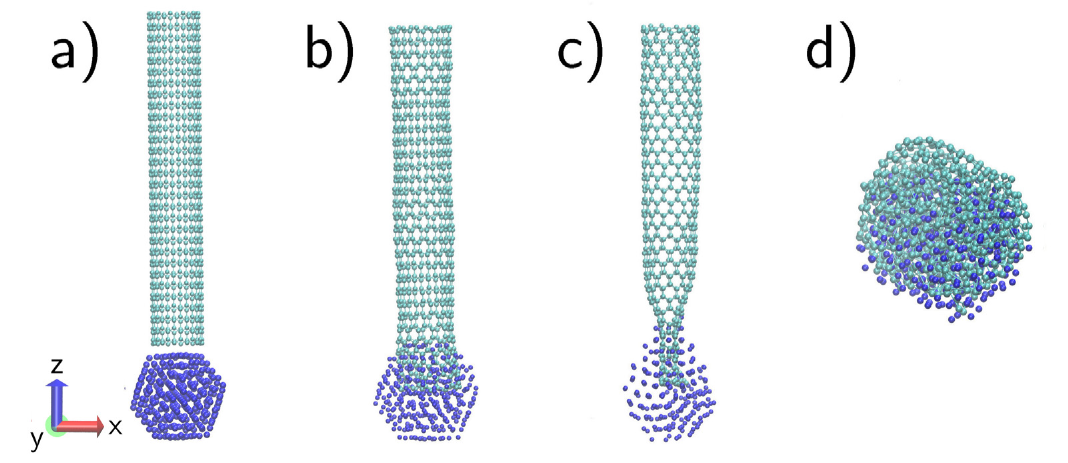
Figure 1: Evolution of the nanotube structure on top of the Ni₃₀₉ nanoparticle at $T=400$ K. Panel (a) shows the initial structure of the system. Panels (b), (c) and (d) illustrate snapshots of the system after 5 ns of simulation at different values of the binding energy between Ni and C atoms: (b) $D_{e}^{\rm Ni-C}=0.2$ eV: the nanotube placed atop the nanoparticle is stable and resembles its original structure; (c) $D_{e}^{\rm Ni-C}=0.8$ eV: the nanotube is stable but the structure of both the nanotube and the nanoparticle is strongly deformed; (d) $D_{e}^{\rm Ni-C}=2.4$ eV: the nanotube is unstable and collapses just after the simulation starts.

In Refs. Yamaguchi_1999_EPJD.9.385 ; Shibuta_2007_ComputMaterSci.39.842 , a many-body potential for the transiti- on-metal–carbon interaction was developed on the basis of density-functional theory (DFT) calculations of small NiC_n ($n=1-3$) clusters. It was noted that the developed potential was a rough estimation, since the introduced parametrization was based on the extrapolation of DFT-based results obtained in the case of small atomic clusters only. Nevertheless, this potential was utilized for a molecular dynamics study of formation of metallofullerenes Yamaguchi_1999_EPJD.9.385 and single-walled carbon nanotubes Shibuta_2007_ComputMaterSci.39.842 . In Ref. Martinez-Limia_2007_JMolModel.13.595 , a similar approach, based on the DFT optimization of small Ni–hydrocarbon systems, was utilized for construction of a more elaborated REBO-type force field, which was applied for simulating the catalyzed growth of single-walled carbon nanotubes on nickel clusters consisting of several tens of atoms.

Alongside with the bond-order many-body potentials, less sophisticated pairwise potentials have been also utilized for studying dynamic processes with nickel-carbon systems. For instance, the pairwise Morse potential was used in Ref. Lyalin_2009_PhysRevB.79.165403 to investigate how thermodynamic properties of a nickel cluster change by the addition of a carbon impurity. The pairwise Morse potential was chosen for the description of the Ni–C interaction because of its simplicity. It allowed to study the influence of the parameters on thermodynamic properties of the C-doped Ni₁₄₇ cluster, maintaining a clear physical picture of the process occurring in the system Lyalin_2009_PhysRevB.79.165403 . For this purpose, the Ni–C interatomic potential, obtained from the results of earlier DFT calculations of small NiC_n ($n=1-3$) clusters Yamaguchi_1999_EPJD.9.385 , was fitted by the Morse potential:

$$U^{\rm Ni-C}(r)=D_{e}\left[\left(1-e^{-\beta(r-R_{e})}\right)^{2}-1\right]\ .$$ (17)

The fitting procedure performed in Ref. Lyalin_2009_PhysRevB.79.165403 resulted in the values of the Ni–C bond dissociation energy $D_{e}^{\rm Ni-C}$ = 2.43 eV, equilibrium distance $R_{e}^{\rm Ni-C}=1.763$ Å, and $\beta=1.869$ Å^-1.

In Ref. Ryu_2010_JPhysChemC.114.2022 , a MD investigation of various noble and transition-metal clusters interacting with graphite was performed. It was stated that such an interaction is mainly dominated by a weak van der Waals force, thus the pairwise Lennard-Jones potential was utilized to model it. The depth of the potential well in the case of the Ni–C interaction was defined as $D_{e}^{\rm Ni-C}=0.023$ eV. In Refs. Shibuta_2007_ComputMaterSci.39.842 and Lin_2007_JMaterProcessTechnol.192.27 , the values of $D_{e}^{\rm Ni-C}=2.478$ eV and 0.1 eV were utilized to model the Ni–C interaction, respectively. Thus, a broad range of interatomic parameters for various nickel-carbon systems have been suggested in the previous studies, although it is hard to conclude from these studies which parameters should be utilized for the description of the stability and growth mechanism of nanotubes. In this paper we elaborate on this issue and justify our choice.

3 Results

3.1 Stability and instability of the system

Following the arguments exploited in Ref. Lyalin_2009_PhysRevB.79.165403 , in the present study we utilize the pairwise Morse potential to describe the interaction between nickel and carbon atoms. In order to investigate the dependence of the system evolution on the parameters of the potential, the depth of the potential well, $D_{e}^{\rm Ni-C}$, was varied in the range from 0.2 to 2.4 eV in steps of 0.2 eV. The geometrical structure of the system simulated at 400 K is presented in Figure 1.

As seen from the figure, stability of the system depends strongly on the binding energy $D_{e}^{\rm Ni-C}$ between the nickel and carbon atoms. Thus, when the Ni–C interaction is covalent but rather weak ($D_{e}^{\rm Ni-C}=0.2$ eV, panel (b)), the nanotube placed on top of the nickel nanoparticle is stable, and the final structure obtained after 5 ns of simulation resembles the initial structure (cf. panel (a)). Increasing the interaction energy up to 0.8 eV (panel (c)), the nanotube still remains stable but its lower part is significantly deformed. One can also observe the deformation of the nanoparticle structure from the icosahedral (panel (a)) to the droplet-like one. Finally, when the dissociation energy of the Ni–C bond exceeds 1.0 eV, the system becomes unstable, and the nanotube collapses during the first 100 ps of the simulation. Panel (d) illustrates the structure of the system simulated with the value $D_{e}^{\rm Ni-C}=2.4$ eV, which was obtained by fitting the results of DFT-based calculations of small NiC_n clusters Yamaguchi_1999_EPJD.9.385 .

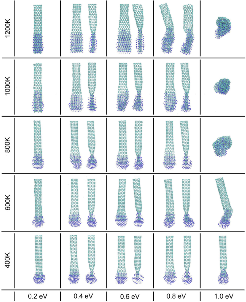
Figure 2: Stability diagram of the single-walled carbon nanotube on top of the nickel nanoparticle depending on the temperature and the interaction energy between Ni and C atoms.

The results of present simulations are in agreement with the findings obtained on the basis of the liquid surface model Solovyov_2008_PhysRevE.78.051601 . Within this model approach, it was found that if the interaction of a nanotube with a catalytic nanoparticle is weak (i.e., the well depth of the Ni–C interatomic potential is less than 1 eV) the longer nanotubes are energetically more favorable. Since the binding energy per atom decreases in this case, attachment of additional atoms is energetically favorable resulting in the nanotube growth. When the nanoparticle-nanotube interaction is strong (e.g., when the well depth $D_{e}^{\rm Ni-C}=1.2$ or 1.5 eV as in Ref. Solovyov_2008_PhysRevE.78.051601 ), the trend of the binding energy per atom changes, and it becomes energetically more favorable for the nanotube to collapse. This critical value of the Ni–C interaction is in very good agreement to the one, which we have determined in this work from MD simulations.

As described above, there have been a number of experimental reports during the last decade on the successful growth of single- and multi-walled carbon nanotubes at various conditions, in particular, at various temperatures. In Figure 2, we present the results of simulations conducted at different temperatures in the range from 400 to 1200 K, that corresponds to the typical range of temperatures at which nanotubes are grown in experiment.

The figure demonstrates that an increase of the Ni–C binding energy leads to the deformation of the lower part of the nanotube that is in contact with the nanoparticle. At $T=600$ K and $D_{e}^{\rm Ni-C}=1.0$ eV the nanotube becomes quasistable and bends from the $z$-axis. Both the lower part of the nanotube and the nanoparticle lose their initial regular structure and form a kind of amorphous nickel-carbon system. Increasing the temperature, the nanotube becomes unstable at $D_{e}^{\rm Ni-C}=1.0$ eV.

Therefore, one can conclude that the carbon nanotube remains stable in the whole range of considered temperatures at comparably large simulation times when the binding energy between Ni and C atoms is about $0.2-0.6$ eV. However, when the energy is equal to or larger than 0.4 eV, the lower part of the nanotube, that is in contact with the nanoparticle, is significantly distorted. Therefore, a highly symmetric structure of the nanotube is kept in the course of simulations at the Ni–C interaction energies of about 0.2 eV.

3.2 Melting of the catalytic nanoparticle

When the interaction between nickel and carbon atoms is weak ($D_{e}^{\rm Ni-C}=0.2$ eV), an increase of the temperature leads to the melting of the nanoparticle and its absorption into the nanotube, as demonstrated in the leftmost column of Figure 2. It is well known that the melting temperature of small metal nanoparticles is significantly lower as compared to that of bulk materials. The decrease of the melting temperature of finite-size systems in comparison with the bulk occurs due to a substantial increase in the relative number of weakly bound atoms on the cluster surface. According to the so-called Pawlow law Pawlow_1909_ZPhysChem.65 , the melting temperature $T_{m}$ of spherical particles possessing a homogeneous surface depends on their radius $R$ as $T_{m}=T_{m}^{\rm bulk}\left(1-\alpha/R\right)$, where $T_{m}^{\rm bulk}$ is the melting temperature of a bulk material Qi_2001_JChemPhys.115.385 ; Lyalin_2009_PhysRevB.79.165403 ; Yakubovich_2013_PhysRevB.88.035438 . Melting of the isolated Ni₃₀₉ nanoparticle simulated with the Finnis-Sinclair potential takes place in a broad temperature range between 900 K and 1400 K, as seen from Figure 3. There, the caloric curve, i.e. the temperature dependence of the time-averaged total energy $\langle E_{\rm tot}\rangle$ of the nanoparticle, and the heat capacity at constant volume, $C_{V}$, defined as a derivative of the internal energy of the system with respect to temperature, are shown.

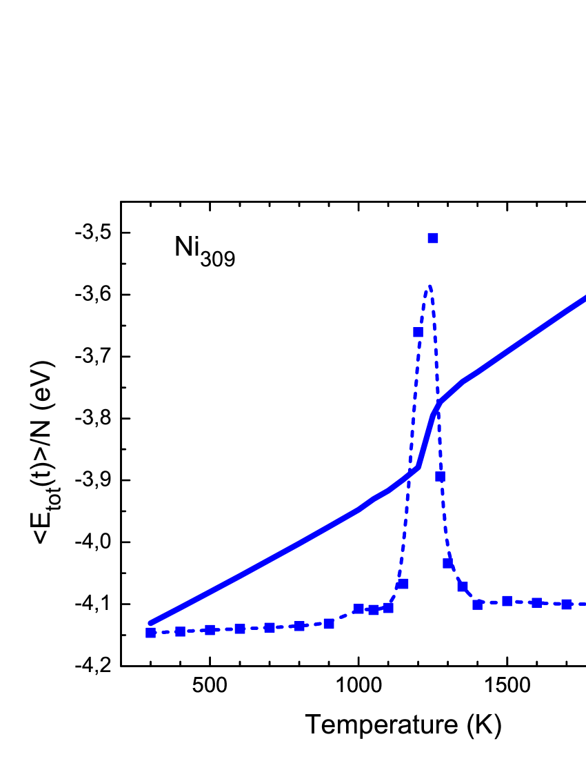
Figure 3: Temperature dependence of the time-averaged total energy $\langle E_{\rm tot}\rangle$ of the isolated Ni₃₀₉ nanoparticle divided by of the number of atoms $N$ (solid curve), and of the heat capacity $C_{V}$ (dashed curve and filled squares). A sharp maximum of the heat capacity at $T=1240$ K arises at the cluster melting temperature.

At $T=1000$ K, the nanoparticle is in the so-called premelted state, when the surface melting of the cluster takes place, while the cluster core remains in the solid phase and resembles its crystalline structure. A small bump in the temperature dependence of the heat capacity indicates for this (see the dashed curve and filled squares in Figure 3). For the Ni₃₀₉ nanoparticle modeled with the Finnis-Sinclair potential the calculated heat capacity curve has a sharp maximum at $T=1240$ K, i.e. at the melting temperature of the cluster. This value is considerably lower than the melting temperature for the bulk nickel, $T_{m}^{\rm bulk}=1728$K, but fits very well the aforementioned dependence of the melting temperature of small nanoparticles on their radius.

In Ref. Lyalin_2009_PhysRevB.79.165403 ; Ding_2004_JVacSciTechnolA.22.1471 it was discussed that alloying transition-metal nanoparticles with carbon leads to a decrease of their melting temperature, that can reach several hundred Kelvin at a carbon concentration of about 10% Ding_2004_JVacSciTechnolA.22.1471 . This phenomenon is illustrated in Figure 4. At $T=400$ and 600 K, the Ni₃₀₉ nanoparticle remains in the solid phase, while the nanotube penetrates further into the nanoparticle as the temperature increases. At $T=800$ K, there is an evidence of the nanoparticle melting, which initiates its absorption by the nanotube. At higher temperatures, $T=1000$ and 1200 K, the nanoparticle is in the molten state, and nickel atoms fill the interior of the nanotube. In this case, the system is stabilized in such a way that nickel atoms are mostly located in the center of carbon rings, as illustrated in the inset of Figure 4.

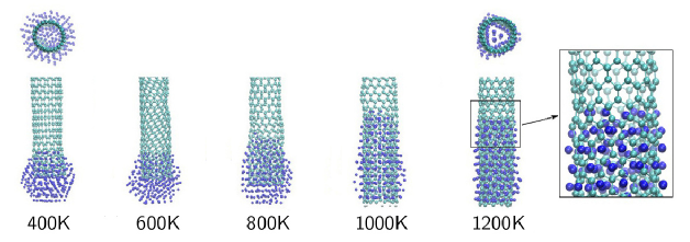
Figure 4: Temperature dependence of the Ni₃₀₉ nanoparticle interacting with a carbon nanotube. Panels illustrate snapshots of the system after 5 ns of simulation with the binding energy between Ni and C atoms $D_{e}^{\rm Ni-C}$ = 0.2 eV.

3.3 Validation of parameters of the Ni–C interaction

In order to validate the parameters of interaction energy between Ni and C atoms that we have utilized in MD simulations, we performed ab initio calculations of the potential energy surface for two Ni–C-based compounds. As a case study, we considered a Ni atom placed in the center of a benzene molecule and of a small carbon ring, and then moved the metal atom away from the carbon systems (see Figure 5). Considering these case studies, we have accounted for different types of Ni–C interaction, that exist when nickel atoms interact either with the nanotube sidewall or with its open end.

The DFT calculations were performed using the hybrid functional composed of the Becke-type gradient-corrected exchange and the gradient-corrected correlation functional of Perdew and Wang (B3PW91) Becke_1993_JChemPhys.98.5648 ; Perdew_1992_PhysRevB.46.6671 . As a basis set, we utilized the correlation-consistent polarized AUG-cc-pVTZ set augmented with diffuse functions Dunning_1989_JChemPhys.90.1007 ; Balabanov_2005_JChemPhys.123.064107 . The calculations were carried out using Gaussian 09 software package g09 .

Performing the potential energy scan, we calculated the binding energy of the systems,

$$E_{b}=E_{\rm Bz/ring}+E_{\rm Ni}-E_{\rm Bz/ring+Ni}\ ,$$ (18)

and then divided the obtained value of $E_{b}$ by the number of carbon atoms. As a result, we calculated the dissociation energy of a single Ni–C bond. Such an approach is valid since the benzene molecule and the carbon ring are highly symmetric structures, and the Ni atom was moved along the main axis of the systems. Thus, each of the Ni–C bonds may be considered as equivalent.

The results of the potential energy scan performed within the above mentioned DFT framework for the case of benzene and for a carbon ring are presented in the left and right panels of Figure 5, respectively. We considered a small carbon ring consisted of 8 atoms that was cut from a narrow $(4,0)$ nanotube. The radius of the ring, calculated after geometry optimization, is 1.65 Å, that is slightly larger than that of the benzene molecule, $R_{\rm Bz}=1.40$ Å. Since the parameters of the Ni–C interaction may depend on the spin state of the system, we studied the singlet (multiplicity $M=1$), triplet ($M=3$) and pentet ($M=5$) states. In the case of the ring, only the singlet state was analyzed, since the higher spin states of the system are unstable.

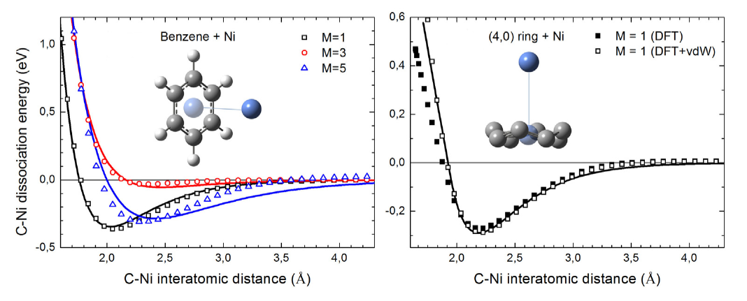
Figure 5: Dependence of the Ni–C bond dissociation energy on the interatomic distance for the case of the Ni–Benzene (left panel) and Ni–carbon ring (right panel) systems. Open symbols illustrate the results of DFT calculations performed at B3PW91/AUG-cc-pVTZ level of theory, corrected by the van der Waals potential. Solid curves represent fitting of the obtained dependencies with the pairwise Morse potential. The potential energy curve obtained from the DFT calculations without the van der Waals-type correction is shown by filled squares. $M$ stands for multiplicity of the system.

As it was discussed earlier (see Ref. Obolensky_2007_IntJQuantChem.107.1335 and references therein), conventional DFT methods cannot account for the van der Waals interaction, which becomes dominant at large interatomic distances. In order to get a better description of the van der Waals interaction between Ni and C atoms, the results of DFT calculations were corrected by a phenomenological van der Waals-type term:

$$E = E_{\rm DFT}+E_{\rm vdW}$$ (19)

$$\equiv E_{\rm DFT}+\epsilon\left[\left(\frac{R_{\rm min}}{r_{ij}}\right)^{12}-2\left(\frac{R_{\rm min}}{r_{ij}}\right)^{6}\right]\ .$$

The $\epsilon\equiv\epsilon({\rm NiC})$ and $R_{\rm min}\equiv R_{\rm min}({\rm NiC})$ functions were constructed as follows:

$$\epsilon({\rm NiC}) = \sqrt{\epsilon({\rm Ni})\cdot\epsilon({\rm C})}\ ,$$

$$R_{\rm min}({\rm NiC}) = \frac{R_{\rm min}({\rm Ni})}{2}+\frac{R_{\rm min}({\rm C})}{2}\ .$$ (20)

For the nickel atom, we utilized the values of $\epsilon({\rm Ni})$ = 0.083 eV and $R_{\rm min}({\rm Ni})$ = 0.63 Å MBN_Explorer1 , while the corresponding parameters for a carbon atom were taken from the CHARMM22 force field: $\epsilon({\rm C})$ = 0.00466 eV and $R_{\rm min}({\rm C})$ = 4.0 Å CHARMM22_FF .

The resulting potential energy curves for the Ni–C interaction, corrected by the introduced above van der Waals-type term, are marked by open symbols in Figure 5. Different spin states of the Benzene-Ni compound affect the depth of the potential well and the equilibrium interatomic distance, ranging from $D_{e}$ = 0.36 eV and $R_{e}$ = 2.05 Å for the singlet state to $D_{e}$ = 0.05 eV and $R_{e}$ = 2.36 Å for the triplet state. In the case of the carbon ring, the calculated values are $D_{e}$ = 0.29 eV and $R_{e}$ = 2.19 Å. For the sake of completeness, the potential energy curve obtained from the DFT calculations without the van der Waals-type correction is shown by filled squares in the right panel of Figure 5. This correction does not affect strongly the behavior of the potential energy curve for the most stable singlet state but should play a much more significant role for the case of less stable states with higher multiplicities. For instance, the value of the van der Waals correction at the equilibrium C–Ni distance is about 0.02 eV which is comparable with $D_{e}$ = 0.05 eV for the triplet state of the Benzene-Ni compound.

Table 2: Parameters of the Morse potential providing the best fit of DFT+vdW potential energy curves for the Ni–C interaction.

	$D_{e}^{\rm Ni-C}$ (eV)	$R_{e}^{\rm Ni-C}$ (Å)	$\beta$ (Å-1)
Bz+Ni: $M=1$	0.345	2.03	2.597
Bz+Ni: $M=3$	0.054	2.46	2.295
Bz+Ni: $M=5$	0.286	2.42	1.667
ring+Ni: $M=1$	0.290	2.19	2.621

The calculated potential-energy dependencies were fitted with pairwise Morse potential parametrization; the resulting curves are shown in Figure 5 by solid lines. The fitting parameters for each case are summarized in Table 2. The presented values of the Ni–C bond dissociation energy correspond well to the value of about 0.2 eV, at which a nanotube atop a nickel nanoparticle turns out to be stable in MD simulations. The other parameters utilized in the simulations, namely the equilibrium distance $R_{e}^{\rm Ni-C}=1.763$ Å and $\beta=1.869$ Å^-1, were taken from Ref. Lyalin_2009_PhysRevB.79.165403 . These values are smaller than most of the corresponding numbers obtained from the DFT calculations (see Table 2). However, such a difference in the values of the geometrical characteristics $R_{e}$ and $\beta$ should not affect significantly the main conclusions made on the basis of the performed MD simulations, as they are mostly determined by the energetic characteristics of the system. This is also supported by the analysis performed in Ref. Lyalin_2009_PhysRevB.79.165403 demonstrating that an increase of the bond length by a factor 1.5, from the equilibrium value up to 2.645 Å, does not change the melting temperature of the C-doped Ni₁₄₇ cluster. Therefore, the difference in 0.5 Å between the bond length utilized in MD simulations and the one obtained from DFT calculations should not affect significantly the conclusions about the thermodynamic and stability properties of a nanotube placed on the nickel nanoparticle made in our work on the basis of the performed MD simulations.

4 Conclusion

In the present study, we have investigated the stability of a carbon nanotube placed on top of the catalytic Ni₃₀₉ nanoparticle by means of classical molecular dynamics simulations. An explicit set of constant-temperature simulations has been performed with the Langevin thermostat in a broad temperature range between 400 and 1200 K, for which a successful growth of single- and multi-walled nanotubes has been achieved experimentally by means of chemical vapor deposition methods.

In the performed simulations, the nickel-carbon interaction has been modeled by a pairwise Morse potential. The influence of the parameters on the thermodynamic and stability properties of the system has been analyzed. It was clearly demonstrated that depending on the parameters of the Ni–C potential different scenarios of the nanotube dynamics atop the nanoparticle are possible. When the Ni–C interaction is relatively weak and does not exceed several tenths of electronvolt, the nanotube placed on top of the nanoparticle is stable and resembles its initial structure in the course of MD simulations. An increase of the interaction energy causes a significant deformation of both the nanotube and the nanoparticle even at relatively low temperature, $T=400$ K. Further increase of the interaction energy leads to the abrupt collapse of the nanotube in the initial stage of simulation.

By means of MD simulations we have demonstrated that at $T=800$ K the nanoparticle, linked to the nanotube, premelts; this, in turn, initiates its absorption by the nanotube. It has been shown that the melting temperature of the isolated Ni₃₀₉ nanoparticle is several hundred Kelvin higher than it is in the case of the nanoparticle linked to a nanotube. It is in agreement with previous findings that alloying transition-metal nanoparticles with carbon leads to a decrease of their melting temperature.

In order to validate the parameters of the Ni–C interaction, utilized in the MD simulations, we have performed a set of DFT calculations of the potential energy of the Ni–C interaction for the two Ni–C-based compounds, namely for a Ni atom placed in the center of (i) a benzene molecule and (ii) a small carbon ring. The results of DFT calculations have been corrected by accounting for the large-distance van der Waals interaction between the Ni and C atoms and analyzed for different spin states of the systems. The calculated dissociation energy of the Ni–C bond corresponds to the values needed for the stability and absence of a noticeable deformation of a nanotube atop a nanoparticle at relatively low temperatures in MD simulations.

In the further work, the validated parameters of the Ni–C interatomic potential can be utilized for simulating the nanotube formation and growth in the presence of a carbon-rich feedstock gas. Usage of the pairwise Morse potential will allow for the study of the atomistic details of the carbon nanotube growth mechanism, keeping a clear physical picture of the processes occurring in the system.

References

- (1) S. Iijima, Nature 354, 56 (1991)
- (2) C. Journet et al., Nature 388, 756 (1997)
- (3) A. Thess et al., Science 273, 483 (1996)
- (4) M. Terrones et al., Nature 388, 52 (1997)
- (5) Y.C. Choi et al., Appl. Phys. Lett. 76, 2367 (2000)
- (6) H. Li, C. Shi, X. Du, C. He, J. Li, N. Zhao, Mater. Lett. 62, 1472 (2008)
- (7) D. Yuan et al., Nano Lett. 8, 2576 (2008)
- (8) J. Kang, J. Li, N. Zhao, X. Du, C. Shi, P. Nash, J. Mater. Sci. 44, 2471 (2009)
- (9) P. Diao, Z. Liu, Adv. Mater. 22, 1430 (2010)
- (10) A. Martinez-Limia, J. Zhao, P.B. Balbuena, J. Mol. Model. 13, 595 (2007)
- (11) P.J.F. Harris, Carbon 45, 229 (2007)
- (12) J. Kang, J. Li, X. Du, C. Shi, N. Zhao, P. Nash, Mater. Sci. Eng. A 475, 136 (2008)
- (13) R. Saito, G. Dresselhaus, M.S. Dresselhaus, Physical Properties of Carbon Nanotubes (Imperial College Press, London, 1998)
- (14) A.R. Harutyunyan, T. Tokune, E. Mora, Appl. Phys. Lett. 87, 051919 (2005)
- (15) H. Kanzow, A. Ding, Phys. Rev. B 60, 11180 (1999)
- (16) J. Gavillet, A. Loiseau, C. Journet, F. Willaime, F. Ducastelle, J.-C. Charlier, Phys. Rev. Lett. 87, 275504 (2001)
- (17) F. Ding, A. Rosen, K. Bolton, J. Chem. Phys. 121, 2775 (2004)
- (18) H. Cui, O. Zhou, B.R. Stoner, J. Appl. Phys. 88, 6072 (2000)
- (19) G.-H. Jeong, N. Satake, T. Kato, T. Hirata, R. Hatakeyama, K. Tohji, Jpn. J. Appl. Phys. 42, L1340 (2003)
- (20) P. Pawlow, Z. Phys. Chem. 65, 1 (1909)
- (21) Y. Qi, T. Çağin, W.L. Johnson, W.A. Goddard III, J. Chem. Phys. 115, 385 (2001)
- (22) A. Lyalin, A. Hussien, A.V. Solov’yov, W. Greiner, Phys. Rev. B 79, 165403 (2009)
- (23) A.V. Yakubovich, G.B. Sushko, S. Schramm, A.V. Solov’yov, Phys. Rev. B 88, 035438 (2013)
- (24) S. Hofmann, C. Ducati, J. Robertson, B. Kleinsorge, Appl. Phys. Lett. 83, 135 (2003)
- (25) N.G. Shang, Y.Y. Tan, V. Stolojan, P. Papakonstantinou, S.R.P. Silva, Nanotechnology 21, 505604 (2010)
- (26) M. He et al., Nano Res. 4, 334 (2011)
- (27) N. Halonen et al., Phys. Stat. Sol. (b) 248, 2500 (2011)
- (28) S. Irle, Y. Ohta, Y. Okamoto, A.J. Page, Y. Wang, K. Morokuma, Nano Res. 2, 755 (2009)
- (29) Y. Ohta, Y. Okamoto, S. Irle, K. Morokuma, Carbon 47, 1270 (2009)
- (30) Y. Shibuta, S. Maruyama, Chem. Phys. Lett. 382, 381 (2003)
- (31) J. Zhao, A. Martinez-Limia, P.B. Balbuena, Nanotechnology 16, S575 (2005)
- (32) J. Tersoff, Phys. Rev. B 37, 6991 (1988)
- (33) D.W. Brenner, Phys. Rev. B 42, 9458 (1990); Erratum: ibid. 46, 1948 (1992)
- (34) R.E. Smalley et al., J. Am. Chem. Soc. 128, 15824 (2006)
- (35) Y. Ohta, Y. Okamoto, S. Irle, K. Morokuma, ACS Nano 2, 1437 (2008)
- (36) I.A. Solov’yov, M. Mathew, A.V. Solov’yov, W. Greiner, Phys. Rev. E 78, 051601 (2008)
- (37) W. Humphrey, A. Dalke, K. Schulten, J. Molec. Graphics 14, 33 (1996)
- (38) I.A. Solov’yov, A.V. Yakubovich, P.V. Nikolaev, I. Volkovets, A.V. Solov’yov, J. Comput. Chem. 33, 2412 (2012)
- (39) http://www.mbnexplorer.com/
- (40) I.A. Solov’yov, A.V. Solov’yov, W. Greiner, A. Koshelev, A. Shutovich, Phys. Rev. Lett. 90, 053401 (2003)
- (41) J. Geng, I.A. Solov’yov, D.G. Reid, P. Skelton, A.E.H. Wheatley, A.V. Solovyov, B.F.G. Johnson, Phys. Rev. B 81, 214114 (2010)
- (42) A.V. Verkhovtsev, A.V. Yakubovich, G.B. Sushko, M. Hanauske, A.V. Solov’yov, Comput. Mater. Sci. 76, 20 (2013)
- (43) A.V. Yakubovich, A.V. Verkhovtsev, M. Hanauske, A.V. Solov’yov, Comput. Mater. Sci. 76, 60 (2013)
- (44) G.B. Sushko, V.G. Bezchastnov, I.A. Solov’yov, A.V. Korol, W. Greiner, A.V. Solov’yov, J. Comput. Phys. 252, 404 (2013)
- (45) V.V. Dick, I.A. Solov’yov, A.V. Solov’yov, Phys. Rev. B 84, 115408 (2011)
- (46) I.A. Solov’yov, A.V. Solov’yov, N. Kébaili, A. Masson, C. Bréchignac, Phys. Stat. Sol. (b) 251, 609 (2013)
- (47) M. Panshenskov, I.A. Solov’yov, A.V. Solov’yov, J. Comput. Chem. (2014), DOI: 10.1002/jcc.23613
- (48) M.W. Finnis, J.E. Sinclair, Philos. Mag. A 50, 45 (1984)
- (49) G.B. Sushko, A.V. Verkhovtsev, A.V. Yakubovich, S. Schramm, A.V. Solov’yov, J. Phys. Chem. A (submitted)
- (50) A.V. Verkhovtsev, G.B. Sushko, A.V. Yakubovich, A.V. Solov’yov, Comput. Theor. Chem. 1021, 101 (2013)
- (51) G.B. Sushko, A.V. Verkhovtsev, A.V. Solov’yov, J. Phys. Chem. A (2014), DOI: 10.1021/jp501723w
- (52) R.P. Gupta, Phys. Rev. B. 23, 6265 (1981)
- (53) A.P. Sutton, J. Chen, Philos. Mag. Lett. 61, 139 (1990)
- (54) M.S. Daw, S.M. Foiles, M.I. Baskes, Mater. Sci. Rep. 9, 251 (1993)
- (55) H. Rafii-Tabar, G. A. Mansoori, in Encyclopedia of Nanoscience and Nanotechnology, Vol. 4, edited by H.S. Nalwa (American Scientific Publishers, Valencia, CA, USA, 2004) pp. 231-248
- (56) F. Cleri, V. Rosato, Phys. Rev. B 48, 22 (1993)
- (57) V. Rosato, M. Guellope, B. Legrand, Philos. Mag. A 59, 321 (1989)
- (58) J.H. Li, X.D. Dai, T.L. Wang, B.X. Liu, J. Phys.: Condens. Matter 17, 086228 (2007)
- (59) M.S. Daw, M.I. Baskes, Phys. Rev. Lett. 50, 1285 (1983)
- (60) M.S. Daw, M.I. Baskes, Phys. Rev. B 29, 6443 (1984)
- (61) D. Tománek, A.A. Aligia, C.A. Balseiro, Phys. Rev. B 32, 5051 (1985)
- (62) W.S. Lai, B.X. Liu, J. Phys.: Condens. Matter 12, L53 (2000)
- (63) Y. Yamaguchi, S. Maruyama, Eur. Phys. J. D 9, 385 (1999)
- (64) Y. Shibuta, S. Maruyama, Comput. Mater. Sci. 39, 842 (2007)
- (65) J.H. Ryu, H.Y. Kim, D.H. Kim, D.H. Seo, H.M. Lee, J. Phys. Chem. C 114, 2022 (2010)
- (66) Z.-C. Lin, J.-C. Huang, Y.-R. Jeng, J. Mater. Process. Technol. 192-193, 27 (2007)
- (67) F. Ding, K. Bolton, A. Rosén, J. Vac. Sci. Technol. A 22, 1471 (2004)
- (68) A.D. Becke, J. Chem. Phys. 98, 5648 (1993)
- (69) J.P. Perdew, J.A. Chevary, S.H. Vosko, K.A. Jackson, M.R. Pederson, D.J. Singh, C. Fiolhais, Phys. Rev. B 46, 6671 (1992)
- (70) R.A. Kendall, T.H. Dunning, Jr., R.J. Harrison, J. Chem. Phys. 96, 6796 (1992)
- (71) N.B. Balabanov, K.A. Peterson, J. Chem. Phys. 123, 064107 (2005)
- (72) M.J. Frisch et al., Gaussian 09, Revision A.01, Gaussian: Wallingford, CT, USA, 2009
- (73) O.I. Obolensky, V.V. Semenikhina, A.V. Solov’yov, W. Greiner, Int. J. Quant. Chem. 107, 1335 (2007)
- (74) A.D. MacKerell, Jr. et al., J. Phys. Chem. B 102, 3586 (1998)