Graph Spectral Properties of
Deterministic Finite Automata

Abstract

We prove that a minimal automaton has a minimal adjacency matrix rank and a minimal adjacency matrix nullity using equitable partition (from graph spectra theory) and Nerode partition (from automata theory). This result naturally introduces the notion of matrix rank into a regular language $L$, the minimal adjacency matrix rank of a deterministic automaton that recognises $L$.

We then define and focus on rank-one languages: the class of languages for which the rank of minimal automaton is one. We also define the expanded canonical automaton of a rank-one language.

1 Introduction

The counting function $C_{L}:\mathbb{N}\rightarrow\mathbb{N}$ of a language $L$ over a finite alphabet maps a natural number $n$ into the number of words in $L$ of length $n$ defined as:

$$C_{L}(n):=|\{w\in L\mid|w|=n\}|.$$

The counting function is a fundamental object in formal language theory and has been studied extensively (cf. [1, 2])． If $L$ is a regular language, we can represent its counting function $C_{L}(n)$ using the $n$-th power of an adjacency matrix of a deterministic automaton that recognises $L$. Our interest is in the “easily countable” class of languages, in the intuitive sense of the word. In this paper, we define and focus on rank-one languages: the class of languages that can be recognised by a deterministic automaton for which the adjacency matrix rank is one.

Counting and its applications For any regular language $L$, it is a well-known result that the counting function of $L$ satisfies:

$$C_{L}(n)=IM^{n}F$$ (1.1)

where $M$ is an adjacency matrix, $I$ is an initial vector and $F$ is a final vector of any deterministic automaton recognises $L$, since $(M^{n})_{ij}$ equals to the number of paths of length $n$ from $i$ to $j$ and this corresponds the number of words of length $n$ (cf. Lemma 1 in [3]). We give the simple example of Equation (1.1) as follows.

Example 1

Let ${\cal A}_{fib}$ is a deterministic automaton recognises $L=(a+ba)^{*}$ and

$$M=\begin{bmatrix}1&1\\ 1&0\end{bmatrix},\;\;\;\;\;\;\;\;\;\;\;\;I=\begin{bmatrix}1&0\end{bmatrix},\;\;\;\;\;\;\;\;\;\;\;\;F=\begin{bmatrix}1\\ 0\end{bmatrix}$$

are its adjacency matrix, initial and final vector. Then the following holds.

$$C_{L}(0) = |\{\varepsilon\}|=1,\;\;\;C_{L}(1)=|\{a\}|=1,$$

$$C_{L}(2) = |\{aa,ba\}|=2,$$

$$\vdots$$

$$C_{L}(n) = IM^{n}F=\begin{bmatrix}1&0\end{bmatrix}\begin{bmatrix}1&1\\ 1&0\end{bmatrix}^{n}\begin{bmatrix}1\\ 0\end{bmatrix}$$ (1.2)

${\cal A}_{fib}$

Equation (1.2) means that $C_{L}(n)$ equals to the $(n+1)$-th Fibonacci number. $\hfill\diamond$

Ranking is one of the variants of counting. The ranking function of $L$ over a finite alphabet $A$ is a bijective function $R_{L}:L\rightarrow\mathbb{N}$ that maps a word $w$ in $L$ to its index in the lexicographic ordering $\prec$ over $A^{*}$ defined as:

$$R_{L}(w):=|\{v\in L\mid v\prec w\}|.$$

In 1985, Goldberg and Sipser introduced a ranking-based string compression in [4]. Recently, the author studied a ranking-based compression on a regular language to analyse its compression ratio and improve a ranking algorithm in [3]. We show an example of a ranking-based compression on a regular language.

Example 2

The formal grammar of Uniform Resource Identifier (URI) is defined in RFC 3986 [5], and it is known that the formal grammar of URI is regular (cf. [6]). Because the language of all URIs $U$ is regular, we can apply a ranking-based compression on a regular language. For example, the index of the URI $w_{1}=$ http://dlt2014.sciencesconf.org/ is:

$$R_{U}(w_{1})=728552296504796066382113700758455910393907656035063493.$$

The word $w_{1}$ is 32 bytes ($|w_{1}|=32$), whereas its index $R_{U}(w_{1})$ is 23 bytes ($\lfloor\log_{256}R_{U}(w_{1})\rfloor=23$). $w_{1}$ is compressed up to $72\%$ and, clearly, we can decompress it by the inverse of $R_{U}$ since ranking is bijective. $\hfill\diamond$

In the case of a ranking on a regular language, the ranking function and its inverse (unranking) of $L$ can be calculated using the adjacency matrix of the deterministic automaton $L$ (cf. [7, 8, 3]). Indeed, Example 2 uses RANS[6], which is open source software implemented by the author based on the algorithms in [3].

The computational complexity of an unranking function is higher than a ranking function because the former requires matrix multiplication but the latter does not (cf. Table 1 in [3]). In Example 2, the calculation of ranking (compression) was performed in less than one second; however, the calculation of unranking (decompression) took about two minutes. The reason for such results is that the cost of matrix multiplication is high (the naive algorithm has cubic complexity), and the unranking algorithm requires matrix multiplications, while the ranking algorithm does not. The minimal automaton of $U$ used in Example 2 has 180 states, and its adjacency matrix multiplication cost is high in practice.

Rank-one languages and our results There are several classes of matrices that have a matrix power that can be computed efficiently (e.g. diagonalisable matrices and low-rank matrices). We focus on rank-one matrices from these classes. As we describe in Section 4, the power of a rank-one matrix has constant time complexity with linear-time preprocessing. We investigate rank-one languages: the class of languages for which the rank of minimal automaton is one. We define an automaton as rank-$n$ if its adjacency matrix is rank-$n$. Next, we introduce the definition of the rank of a language.

Definition 1

A regular language $L$ is rank-$n$ if there exists a rank-$n$ deterministic automaton that recognises $L$, and there does not exist a rank-$m$ deterministic automaton that recognises $L$ for any $m$ less than $n$. $\hfill\diamond$

However, Definition 1 raises the question of how to find a minimal rank. It is a classical theorem in automata theory that for any regular language $L$, there is a unique automaton ${\cal A}$ that recognises $L$ that has a minimal number of states, and ${\cal A}$ is called the minimal automaton of $L$. We intend to refine Definition 1 as the following definition.

Definition 1 (refined)

A regular language $L$ is rank-$n$ if its minimal automaton is rank-$n$. $\hfill\diamond$

Nevertheless, to achieve this we have to show that a minimal automaton has the minimal rank for consistency of the above two definitions. Hence in Section 3, we prove the following theorem, which has a more general statement.

Theorem 1.1

An automaton ${\cal A}$ is minimal if and only if both the rank and the nullity of its adjacency matrix are minimal. $\hfill\diamond$

Theorem 1.1 provides a necessary and sufficient condition for the minimality of an automaton and is a purely algebraic characterisation of minimal automata. This theorem is not obvious because, in general, for an automaton ${\cal A}$, the number of states of ${\cal A}$ and the rank (nullity) of ${\cal A}$ are not related. This is illustrated in Figure 1, where the deterministic automaton ${\cal B}_{1}$ has three states and its rank is two, whereas ${\cal C}_{1}$ has four states and its rank is one, which equals the rank of the minimal automaton ${\cal A}_{1}$. Therefore, we can-not argue naively that “any minimal automaton has the minimal rank (nullity)” by its minimality of states.

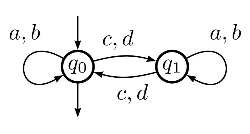
${\cal A}_{1}$

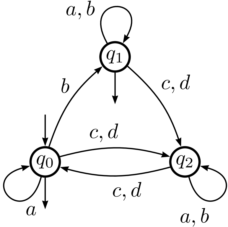
${\cal B}_{1}$

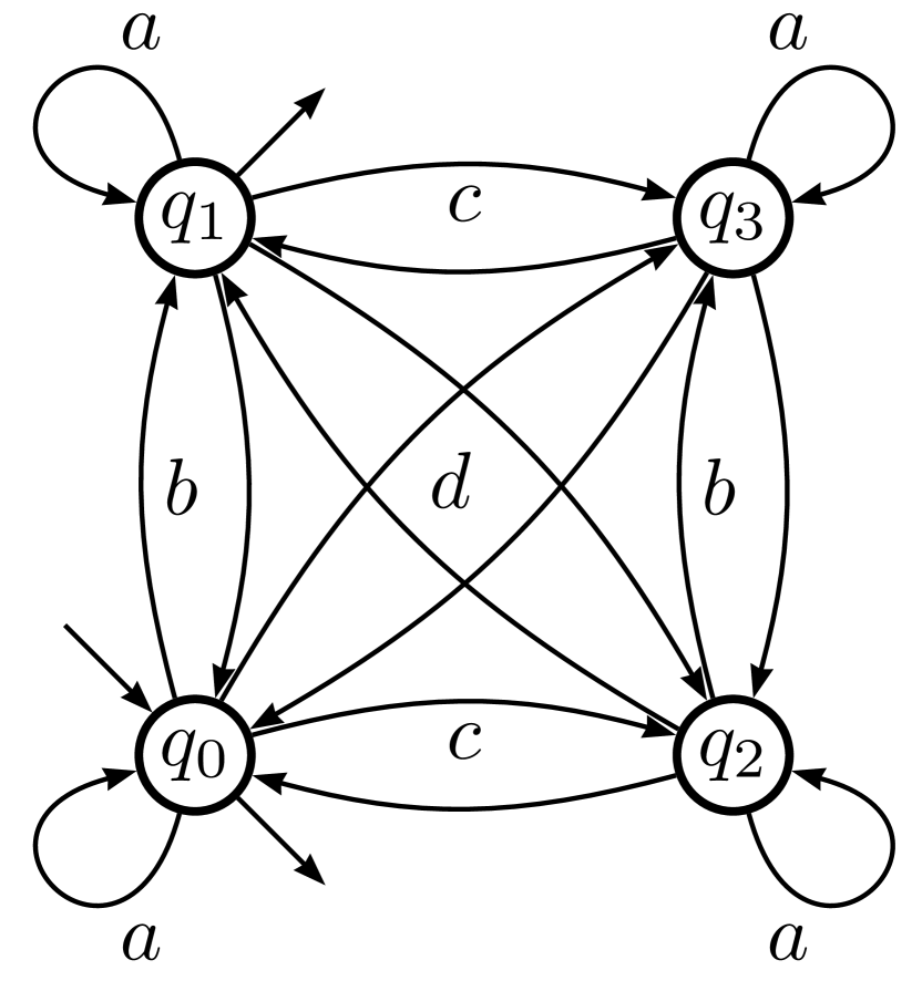
${\cal C}_{1}$

$$M({\cal A}_{1})=\begin{bmatrix}2&2\\ 2&2\end{bmatrix}\;\;\;\;\;\;\;\;\;\;\;\;\;\;M({\cal B}_{1})=\begin{bmatrix}1&1&2\\ 0&2&2\\ 2&0&2\end{bmatrix}\;\;\;\;\;\;\;\;\;\;\;\;\;\;\;\;\;\;\;M({\cal C}_{1})=\begin{bmatrix}1&1&1&1\\ 1&1&1&1\\ 1&1&1&1\\ 1&1&1&1\end{bmatrix}$$

Figure 1: Three equivalent deterministic trim automata and these adjacency matrices.

The proof consists of the use of two fundamental tools: equitable partition from graph spectra theory and Nerode partition from automata theory. We briefly introduce these two partitions in Section 2, then give the proof of Theorem 1.1 in Section 3. In Section 4, we investigate the properties of rank-one languages and introduce expanded canonical automata. In Section 5 we briefly discuss three topics that are not yet understood or lack maturity.

2 Nerode partition and equitable partition

We assume that the reader has a basic knowledge of automata, graphs and linear algebra. All results in this section are well-known, and for more details, we refer the reader to [9] for automata theory and [10] for graph spectra theory.

2.1 Automata and languages

A deterministic finite automaton ${\cal A}$ is a quintuple ${\cal A}=\langle Q,A,\delta,q_{0},F\rangle$; the finite set of states $Q$, the finite set $A$ called alphabet, the transition function $\delta:Q\times A\rightarrow Q$, the initial state $q_{0}$, and the set of final states $F\subseteq Q$. If $\delta(q,w)=p$ is a transition of automaton ${\cal A}$, $w$ is said to be the label of the transition. We call a transition $\delta(p,w)=q$ is successful if its destination is in the final states $F$ of ${\cal A}$. A word $w$ in $A^{*}$ is accepted by ${\cal A}$ if it is the label of a successful transition from the initial state of ${\cal A}$: $\delta(q_{0},w)\in F$. The symbol like $|{\cal A}|$ denotes the number of states $|Q|$ for an automaton ${\cal A}$. The set of all acceptable words of ${\cal A}$, or language of ${\cal A}$, is denoted by $L({\cal A})$. We call two automata are equivalent if their languages are identical. An deterministic automaton ${\cal A}=\langle Q,A,\delta,q_{0},F\rangle$ is trim if, for all state $q\in Q$, there exist two words $v$ and $w$ such that $\delta(q_{0},v)=q$ (accessible) and $\delta(q,w)\in F$ (co-accessible).

2.2 Graphs and adjacency matrices

A multidigraph $G$ is a pair $G=\langle N,E\rangle$; the set of nodes $N$, the multiset of edges $E$. The adjacency matrix $M(G)$ of $G$ is the $|N|$-dimensional matrix defined as:

$$M(G)_{ij}:=\text{the number of edges from node}\;i\;\text{to node}\;j.$$

The spectrum of a matrix $M$ is the multiset of the eigenvalues of $M$ and is denoted by $\lambda(M)$. The kernel of a matrix $M$ is the subspace defined as $\{\bm{v}\mid M\bm{v}=\bm{0}\}$, and is denoted $\ker(M)$. We denote the dimension, rank and nullity (the dimension of the kernel) of $M$ by $\mathrm{dim}(M),\mathrm{rank}(M)$ and $\mathrm{null}(M)$ respectively. The following dimension formula is known as the rank-nullity theorem:

$$\mathrm{dim}(M)=\mathrm{rank}(M)+\mathrm{null}(M).$$

A partition $\pi$ of a multidigraph $G=\langle N,E\rangle$ is a set of nodal sets $\pi=\{C_{1},C_{2},\ldots,C_{k}\}$ that satisfies the following three conditions:

$$\emptyset\notin\pi\;\;\;\text{and}\;\;\;\displaystyle\bigcup_{C\in\pi}C=N\;\;\;\text{and}\;\;\;\forall i,j\in[1,k],i\neq j\Rightarrow C_{i}\cap C_{j}=\emptyset.$$

We call ${}_{\pi}M$ as the partitioned matrix induced by $\pi$ of $M$, that is partitioned as

$${}_{\pi}M=\begin{bmatrix}M_{1,1}&&\cdots&&M_{1,k}\\ \vdots&&&&\vdots\\ M_{k,1}&&\cdots&&M_{k,k}\end{bmatrix}$$ (2.1)

where the block matrix $M_{i,j}$ is the submatrix of $M$ formed by the rows in $C_{i}$ and the columns in $C_{j}$. The characteristic matrix $S$ of $\pi$ is the $|N|\times k$ matrix that is defined as follows:

$$S_{ij}=\begin{cases}1&\text{if}\;i\in C_{j},\\ 0&\text{otherwise}.\end{cases}$$

In general, $S$ is a full rank matrix ($\mathrm{rank}(S)=\min(|N|,k)=k$) and $S^{T}S=\mathrm{diag}(|C_{1}|,|C_{2}|,\ldots,|C_{k}|)$ where $S^{T}$ is the transpose of $S$. The quotient matrix $M^{\pi}$ of $M$ by $\pi$ is defined as the $k\times k$ matrix:

$$M^{\pi}=(S^{T}S)^{-1}S^{T}MS$$ (2.2)

where $(S^{T}S)^{-1}=\mathrm{diag}(\frac{1}{|C_{1}|},\frac{1}{|C_{2}|},\ldots,\frac{1}{|C_{k}|})$. That is, $(M^{\pi})_{ij}$ denotes the average row sum of the block matrix $({}_{\pi}M)_{i,j}$, in the intuitive sense of the word.

Example 3

Consider the deterministic automaton ${\cal B}_{1}$ in Figure 1. Let $\pi_{1}$ be the partition of ${\cal B}_{1}$: $\pi_{1}=\{\{q_{0},q_{1}\},\{q_{2}\}\}$, then its characteristic matrix $S$ and $S^{T}S$, the partitioned matrix ${}_{\pi_{1}}M({\cal B}_{1})$ and the quotient matrix $M({\cal B}_{1})^{\pi_{1}}$ are follows:

$$S=\begin{bmatrix}1&0\\ 1&0\\ 0&1\\ \end{bmatrix},\;\;\;S^{T}S=\begin{bmatrix}2&0\\ 0&1\end{bmatrix},\;\;\;{}_{\pi_{1}}M({\cal B}_{1})=\begin{bmatrix}\begin{bmatrix}\vspace{-.2em}1&1\vspace{-.2em}\\ 0&2\vspace{-.2em}\end{bmatrix}&\begin{bmatrix}\vspace{-.2em}2\vspace{-.2em}\\ 2\vspace{-.2em}\end{bmatrix}\\[5.0pt] \begin{bmatrix}2&0\vspace{-.2em}\\ \end{bmatrix}&\begin{bmatrix}\vspace{-.2em}2\end{bmatrix}\end{bmatrix},\;\;\;M({\cal B}_{1})^{\pi_{1}}=\begin{bmatrix}2&2\\ 2&2\end{bmatrix}.$$

$\hfill\diamond$

2.3 Nerode partition

Because an automaton ${\cal A}$ can be regarded as a multidigraph, we can naturally define the adjacency matrix, partitions and these quotient of ${\cal A}$ as the same manner. Let $q$ be a state of ${\cal A}$. We denote by $F(q)$ the set of words $w$ that are labels of a successful transition starting from $q$. It is called the future of the state $q$. Two states $p$ and $q$ are said to be Nerode equivalent if and only if $F(p)=F(q)$. Nerode partition is the partition induced by Nerode equivalence.

Nerode’s theorem states that states of minimal automaton are blocks of Nerode partition, edges and terminal states are defined accordingly (cf. [11, 12]). That is, note that the adjacency matrix of a minimal automaton equals the quotient matrix of the adjacency matrix of an equivalent automaton by its Nerode partition. For example, $\pi_{1}$ in Example 3 is the Nerode partition of ${\cal B}_{1}$ in Figure 1 and its induced quotient matrix $M({\cal B}_{1})^{\pi_{1}}$ is identical to the adjacency matrix $M({\cal A}_{1})$ of the minimal automaton ${\cal A}_{1}$ in the same figure.

2.4 Equitable partition

If the row sum of each block matrix $M_{i,j}$ in Equation (2.1) induced by $\pi$ is constant, then the partition $\pi$ is called equitable. In that case the characteristic matrix $S$ of $\pi$ satisfies the following equation (cf. Article 15 in [10]):

$$MS=SM^{\pi}$$ (2.3)

If $\bm{v}$ is an eigenvector of $M^{\pi}$ belonging to the eigenvalue $\lambda$, then $S\bm{v}$ is an eigenvector of $M$ belonging to the same eigenvalue $\lambda$. Indeed, left-multiplication of the eigenvalue equation $M^{\pi}\bm{v}=\lambda\bm{v}$ by $S$ yields:

$$\lambda S\bm{v}=(SM^{\pi})\bm{v}=(MS)\bm{v}=M(S\bm{v}).$$

For example, we can verify that $\pi_{1}$ in Example 3 is equitable. We conclude the the following lemma.

Lemma 1

Let $\pi$ be an equitable partition of a matrix $M$ and $M^{\pi}$ be its induced quotient matrix, then $\lambda(M^{\pi})\subseteq\lambda(M)$ holds. ∎

Remark 1

Though many literature of graph spectra theory including [10] treat the notion of equitable partition on simple graphs, the properties of equitable partition including Equation (2.3) and Lemma 1 are also holds on multidigraphs without problems (cf. [13]; Theorem 4.5).

The concept of equitable partition was introduced in [14]. Equitable partition have been considered in the literature also under the name divisor and for more information the reader is referred to Chapter 4 in [13], where basic properties of divisor can be found. $\hfill\diamond$

3 Minimal properties of minimal automata

The “if” direction of the Theorem 1.1 is obvious from the rank-nullity theorem. For proving the “only if” direction, we prove the following two propositions.

1. Quotient by an equitable partition always reduces the dimension, rank and nullity, respectively (Proposition 3.1).

2. Nerode partition is equitable (Proposition 3.2).

Because, as we mentioned in Section 2.3, the adjacency matrix of a minimal automaton equals to the quotient matrix of the adjacency matrix of any equivalent automaton by its Nerode partition.

Proposition 3.1

Let $\pi$ be an equitable partition of a matrix $M$ and $M^{\pi}$ be its induced quotient matrix, then the following inequalities hold.

$$\mathrm{dim}(M^{\pi})\leq\mathrm{dim}(M),\;\;\;\mathrm{rank}(M^{\pi})\leq\mathrm{rank}(M),\;\;\;\mathrm{null}(M^{\pi})\leq\mathrm{null}(M).$$

Proof

$\mathrm{dim}(M^{\pi})\leq\mathrm{dim}(M)$ is obvious, then we prove the rest two inequalities.

Let $\bm{v}$ be a vector in the kernel of $M^{\pi}$ and $\bm{w}$ be a vector not in the kernel of $M^{\pi}$, then the following equations hold.

$$MS\bm{v}=S(M^{\pi}\bm{v})=\bm{0},$$ (3.1)

$$MS\bm{w}=S(M^{\pi}\bm{w})\neq\bm{0}.$$ (3.2)

Equation (3.2) is induced by $M^{\pi}\bm{w}\neq\bm{0}$ and $S\bm{u}\neq\bm{0}$ for any $\bm{u}\neq\bm{0}$ since $S$ has full rank. Equation (3.1) and (3.2) leads:

$$\bm{v}\in\ker(M^{\pi})\Rightarrow S\bm{v}\in\ker(M)\;\;\;\text{and}\;\;\;\bm{w}\not\in\ker(M^{\pi})\Rightarrow S\bm{w}\not\in\ker(M).$$

For any linearly independent vectors $\bm{u}$ and $\bm{u}^{\prime}$ then $S\bm{u}$ and $S\bm{u}^{\prime}$ are also linearly independent since $S$ has full rank. This shows the rest two inequalities. ∎

Proposition 3.2

Nerode partition is equitable.

Proof

Let ${\cal A}=\langle Q,A,\delta,q_{0},F\rangle$ be a deterministic automaton and its Nerode partition $\pi=(C_{1},C_{2},\ldots,C_{k});C_{i}\subseteq Q$. We prove by contradiction.

Assume $\pi$ is not equitable, then there exist $C_{i}$ and $C_{j}$ in $\pi$ and $p$ and $q$ in $C_{i}$ such that $p$ and $q$ have different number of transition rules into $C_{j}$. We assume without loss of generality that the number of transition rules into $C_{j}$ of p is larger than $q$’s. Then there exists at least one alphabet $a$ in $A$ such that $\delta(p,a)\in C_{j}$ and $\delta(q,a)\notin C_{j}$. Let $p_{a}=\delta(p,a)$ and $q_{a}=\delta(q,a)$, then $p_{a}$ and $q_{a}$ are not Nerode equivalent since $p_{a}$ belongs to another partition of $q_{a}$’s. Hence $F(p_{a})\neq F(q_{a})$ holds and either $F(p_{a})$ or $F(q_{a})$ is not empty. We assume without loss of generality that $F(p_{a})$ is not empty. Because $F(p_{a})\neq F(q_{a})$ and $F(p_{a})\neq\emptyset$, there exists $w$ in $F(p_{a})$ such that $w\notin F(q_{a})$ and then $w$ satisfies:

$$\delta(p,aw)=\delta(p_{a},w)\in F\;\;\;\;\text{and}\;\;\;\;\delta(q,aw)=\delta(q_{a},w)\notin F.$$

This leads that $p$ and $q$ are not Nerode equivalent even though $p$ and $q$ belong to the same Nerode equivalent class $C_{i}$. This is contradiction. ∎

It is also proved that any deterministic automaton includes the spectrum of its equivalent minimal automaton by Proposition 3.2 and Lemma 1.

4 Rank-one languages and expanded canonical automata

In this section, we focus on rank-one languages and introduce expanded canonical automata. Firstly, we introduce the well-known general properties of rank-one matrices (cf. Proposition 1 in [15]).

Property 1 (characterization of a rank one matrix)

Let $M$, $n\geq 2$, be a $n$-dimensional real matrix of rank one. Then

1. There exists $\bm{x},\bm{y}$ vectors in $\mathbb{C}^{n};\bm{x},\bm{y}\neq\bm{0}$ such that $M=\bm{x}\bm{y}^{T}$;

2. $M$ has at most one non-zero eigenvalue with algebraic multiplicity 1;

3. This eigenvalue is $\bm{y}^{T}\bm{x}$.$\hfill\diamond$

Property 1 shows that, for any rank-one language $L$, its counting function can be represented as a monomial: $C_{L}(n)=\alpha\lambda^{n}$ for $n>0$ and natural numbers $\alpha$ and $\lambda$. In addition, rank-one matrices have beneficial property that their power can be computable in constant time with linear-time preprocessing. Indeed, for any $m$-dimensional rank-one matrix $M$, there exists $x,y$ such that $xy^{T}=M$ hence, the following equation holds for $\lambda=y^{T}x$:

$$M^{n}=(\bm{x}\bm{y}^{T})^{n}=\bm{x}(\bm{y}^{T}\bm{x})^{n-1}\bm{y}^{T}=\lambda^{n-1}\bm{x}\bm{y}^{T}=\lambda^{n-1}M.$$

This shows that $(M^{n})_{ij}$ equals $\lambda^{n-1}(\bm{x}\bm{y}^{T})_{ij}$, and the inner product of $\bm{x}$ and $\bm{y}$ has linear-time complexity with respect to its dimension $m$.

4.1 In-vector and out-vector

For any rank-one matrix $M$, we can construct $\bm{x}$ and $\bm{y}$ such that $M=\bm{x}\bm{y}^{T}$ from the ratio of the number of incoming edges and outgoing edges, respectively.

Definition 2

Let M be an $n$-dimensional rank-one matrix. The in-vector of $M$ is a non-zero row vector having minimum length in $M$ and is denoted by $\mathrm{in}(M)$. Because $M$ is rank-one, each row vector $\bm{v}_{i}$ in $M$ can be represented as $\bm{v}_{i}=\alpha_{i}\cdot\mathrm{in}(M)$ for some natural number $\alpha_{i}\geq 1$. The out-vector of $M$ is the $n$-dimensional column vector that has an $i$-th element defined as the above coefficient $\alpha_{i}$ and denoted by $\mathrm{out}(M)$.

By this construction, it is clear that an in-vector and out-vector satisfy $\mathrm{out}(M)\cdot\mathrm{in}(M)=M$.

$\hfill\diamond$

In general, an automaton ${\cal A}$ may have the state $q$ such that there are no transition rules into $q$. Hence, the in-vector must be taken from non-zero vectors in the given matrix. We note that, for any rank-one matrix $M$, the out-vector of $M$ always contains one because it consists of the coefficients of the in-vector of $M$ (cf. Example 4).

Example 4

Consider the rank-one automaton shown in the adjacent figure.

This automaton is deterministic and trim. Its adjacency matrix $M$ and in-vector $\mathrm{in}(M)$ and out-vector $\mathrm{out}(M)$ are follows.

$$M=\begin{bmatrix}0&2&1\\ 0&4&2\\ 0&2&1\end{bmatrix},\;\;\;\mathrm{in}(M)=\begin{bmatrix}0,2,1\end{bmatrix},\;\;\;\mathrm{out}(M)=\begin{bmatrix}1\\ 2\\ 1\end{bmatrix}.$$

Note that $\mathrm{in}(M)_{0}=0$ means that $q_{0}$ has no incoming transition rules. $\hfill\diamond$

4.2 Expanded canonical automata

First, we define a normal form of a rank-one automaton.

Definition 3

A rank-one automaton ${\cal A}$ is expanded normal if for its adjacency matrix $M$, each element of the in-vector of $M$ equals to zero or one. $\hfill\diamond$

The automaton in Figure 4 is not expanded normal because the second element of its in-vector equals two. Expanded normal form is a graph normal form of automata, and does not consider labels.

Secondly, we propose the operation expansion that expands the given matrix (graph or automaton) algebraically.

Definition 4

Let ${}^{\pi}M$ and $M$ be two matrices of dimension $m$ and $n$, respectively. We define ${}^{\pi}M$ as an expansion of M if there exists a partition $\pi=\{C_{1},C_{2},\ldots,C_{n}\}$ of ${}^{\pi}M$ such that the characteristic matrix $S$ of $\pi$ satisfies:

$${}^{\pi}M=SM(S^{T}S)^{-1}S^{T}.$$

$\hfill\diamond$

Expansion is an algebraic transformation that increases the dimension of the given matrix. Intuitively, expansion can be regarded as an inverse operation of quotient. Indeed, for any expanded matrix ${}\pi M$ of some $n$-dimensional $M$ by $\pi$ and its characteristic matrix $S$, we have the following equation:

$$({}^{\pi}M)^{\pi}=(S^{T}S)^{-1}S^{T}({}^{\pi}M)S=(S^{T}S)^{-1}S^{T}\left(SM(S^{T}S)^{-1}S^{T}\right)S=M$$

which holds by Equation (2.2) and Definition 4. If $M$ is rank-one, then for any expanded matrix ${}^{\pi}M$ of $M$, the out-vector of ${}^{\pi}M$ consists of same elements as those of the out-vector of $M$. This reflects the invariance of the number of outgoing transition rules of the Nerode equivalent states (cf. Figure 2).

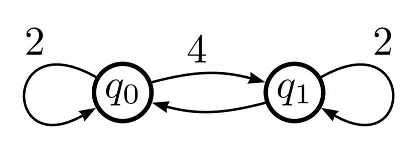
${\cal D}_{1}$

$\xrightarrow{\text{Expand by}\;\{\{q_{0}\},\{q_{1},q^{\prime}_{1}\}\}\;\;}$ $\xleftarrow[\text{Quotient by}\;\{\{q_{0}\},\{q_{1},q^{\prime}_{1}\}\}]{}$

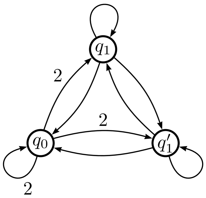
${}^{\pi}{\cal D}_{1}$

$$\begin{bmatrix}2&4\\ 1&2\end{bmatrix}=\begin{bmatrix}2\\ 1\end{bmatrix}\begin{bmatrix}1&2\end{bmatrix}\;\;\;\;\;\;\;\;\;\;\;\;\;\;\;\;\;\;\;\;\;\;\;\;\;\;\;\;\;\;\;\;\;\;\;\;\;\;\;\;\;\;\;\;\;\;\;\;\;\;\;\;\;\;\;\;\begin{bmatrix}2&2&2\\ 1&1&1\\ 1&1&1\end{bmatrix}=\begin{bmatrix}2\\ 1\\ 1\end{bmatrix}\begin{bmatrix}1&1&1\end{bmatrix}$$

Figure 2: The rank-one graph ${\cal D}_{1}$ and its expanded canonical form ${}^{\pi}{\cal D}_{1}$.

Finally, we define a canonical automaton of a rank-one language: expanded canonical automaton. The minimal automaton of a regular language $K$ is uniquely determined by $K$, whereas the expanded canonical automaton of a rank-one language $L$ is not uniquely determined, but its graph structure is uniquely determined by $L$.

Definition 5

Let $L$ be a rank-one language, then we define its expanded canonical automaton ${}^{\pi}{\cal A}_{L}$ as the expanded automaton of the minimal automaton ${\cal A}_{L}$ of $L$ by a partition $\pi=\{C_{1},C_{2},\ldots C_{|{\cal A}_{L}|}\}$ such that, for all $C_{i}\in\pi$, $|C_{i}|=\mathrm{in}({\cal A}_{L})_{i}$ if $\mathrm{in}({\cal A}_{L})_{i}\neq 0$ and 1 otherwise. $\hfill\diamond$

By the definition, it is clear that for any rank-one language $L$, its expanded canonical automaton is expanded normal (cf. Figure 2, or ${\cal A}_{1}$ and its expanded canonical automaton ${\cal C}_{1}$ in Example 1). As we describe in Section 5.1, we introduce expanded canonical automata for analysis and evaluation of the closure properties of rank-one languages. Because of the limitations of space, a detailed discussion of expanded canonical automata is not possible here.

5 The way for further developments

5.1 Closure property of rank-one languages and decomposability

It is natural to consider the closure properties of rank-one languages. However, with some exceptions (e.g. quotient, prefix), the class of lank-one languages is, for the most part, not closed under an operation on languages: e.g. union, concatenation and Kleene star. Indeed, for the two rank-one (expanded canonical) automaton ${\cal E}_{1}$ and ${\cal F}_{1}$ in Figure 3, the union of $L({\cal E}_{1})$ and $L({\cal F}_{1})$ has the spectrum $\{3,2,-1,-1,-1\}$ (without zeros) and is rank-five. We note that $L({\cal E}_{1})$ and $L({\cal F}_{1})$ have the same prefix, and the minimal automaton of $L({\cal E}_{1})\cup L({\cal F}_{1})$ is strongly connected and has nine states. In addition, note that there exist rank-one languages $KandL$ such that the union language $K\cup L$ has irrational and complex eigenvalues.

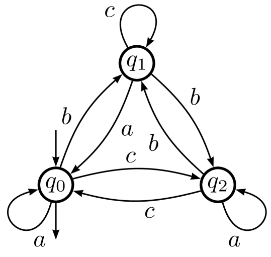
${\cal E}_{1}$

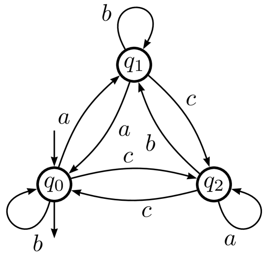
${\cal F}_{1}$

Figure 3: Two rank-one automata (expanded canonical automata).

Conversely, we consider the closure of rank-one languages with an operation on languages or decomposability into rank-one languages (rank-one decomposition). In the case of matrices, matrix rank-one decomposition is well studied and there exist fundamental results such as orthogonal decomposition for real symmetric matrices. We are interested in investigating regular language rank-one decomposition.

5.2 Rank of unambiguous automata

The class of unambiguous automata is a more general class of automata than the class of deterministic automata (cf. [9]). We intend to generalise Definition 1 as Definition 6 which is more essential for the counting structure of languages because unambiguous automata is the most general class that satisfies Equality (1.1). It will be interesting to determine whether the rank of a minimal unambiguous automaton is minimal. If so, we can refine Definition 6 in a similar manner.

Definition 6

A regular language $L$ is unambiguous rank-$n$ if there exists a rank-$n$ unambiguous automaton recognises $L$ and does not exist a rank-$m$ unambiguous automaton recognises $L$ for any $m$ less than $n$. $\hfill\diamond$

5.3 Relation between the conjugacy of automata

Béal et al. developed the theory of conjugacy of automata (cf. [16, 17]) that gives structural information on two equivalent $\mathbb{K}$-automata. Conjugacy of automata is a theory based on matrices, and we think some results in this paper may be reconstructed by the theory of conjugacy.

Acknowledgement I would like to thank my adviser, Kazuyuki Shudo, for his continuous support and encouragement. Special thanks also go to Yuya Uezato, is a postgraduate student at University of Tsukuba, who provided carefully considered feedback and valuable comments.

References

- [1] Shur, A.M.: Combinatorial complexity of regular languages. In: Proceedings of the 3rd International Conference on Computer Science: Theory and Applications. CSR’08, Berlin, Heidelberg, Springer-Verlag (2008) 289–301
- [2] Shur, A.M.: Combinatorial characterization of formal languages. CoRR abs/1010.5456 (2010)
- [3] Sin’ya, R.: Text compression using abstract numeration system on a regular language. Computer Software 30(3) (2013) 163–179 in Japanese, English extended abstract is available at http://arxiv.org/abs/1308.0267.
- [4] Goldberg, A., Sipser, M.: Compression and ranking. In: Proceedings of the Seventeenth Annual ACM Symposium on Theory of Computing. STOC ’85, New York, NY, USA, ACM (1985) 440–448
- [5] Berners-Lee, T., Fielding, R., Masinter, L.: Rfc 3986, uniform resource identifier (uri): Generic syntax (2005)
- [6] Sin’ya, R.: Rans : More advanced usage of regular expressions. http://sinya8282.github.io/RANS/
- [7] Choffrut, C., Goldwurm, M.: Rational transductions and complexity of counting problems. Mathematical Systems Theory 28(5) (1995) 437–450
- [8] Lecomte, P., Rigo, M.: Combinatorics, Automata and Number Theory. 1st edn. Cambridge University Press, New York, NY, USA (2010) Chapter 3: Abstract numeration systems.
- [9] Sakarovitch, J.: Elements of Automata Theory. Cambridge University Press, New York, NY, USA (2009)
- [10] Mieghem, P.V.: Graph Spectra for Complex Networks. Cambridge University Press, New York, NY, USA (2011)
- [11] Nerode, A.: Linear automaton transformations. Proceedings of the American Mathematical Society 9(4) (1958) 541–544
- [12] Béal, M.P., Crochemore, M.: Minimizing incomplete automata. In: Finite-State Methods and Natural Language Processing (FSMNLP’08). Joint Research Center (2008) 9–16
- [13] Cvetković, D.M., Doob, M., Sachs, H.: Spectra of Graphs: Theory and Application. Academic Press, New York (1980)
- [14] Schwenk, A.: Computing the characteristic polynomial of a graph. In Bari, R., Harary, F., eds.: Graphs and Combinatorics. Volume 406 of Lecture Notes in Mathematics. Springer Berlin Heidelberg (1974) 153–172
- [15] Osnaga, S.M.: On rank one matrices and invariant subspaces. Balkan Journal of Geometry and its Applications (BJGA) 10(1) (2005) 145–148
- [16] Béal, M.P., Lombardy, S., Sakarovitch, J.: On the equivalence of z-automata. In: Proceedings of the 32Nd International Conference on Automata, Languages and Programming. ICALP’05, Berlin, Heidelberg, Springer-Verlag (2005) 397–409
- [17] Béal, M.P., Lombardy, S., Sakarovitch, J.: Conjugacy and equivalence of weighted automata and functional transducers. In: Proceedings of the First International Computer Science Conference on Theory and Applications. CSR’06, Berlin, Heidelberg, Springer-Verlag (2006) 58–69