1 Introduction
In this paper we derive a correct expression for the normal ordering of the unitary group
U t = e i H ^ t subscript 𝑈 𝑡 superscript 𝑒 𝑖 ^ 𝐻 𝑡 U_{t}=e^{i\widehat{H}t}
H ^ = i 2 ( ( a † , A a † ) − ( a , A ¯ a ) ) + ( a † , B a ) + i ( a † , h ) − i ( a , h ¯ ) = H ^ 2 + H ^ 1 , ^ 𝐻 𝑖 2 superscript 𝑎 † 𝐴 superscript 𝑎 † 𝑎 ¯ 𝐴 𝑎 superscript 𝑎 † 𝐵 𝑎 𝑖 superscript 𝑎 † ℎ 𝑖 𝑎 ¯ ℎ subscript ^ 𝐻 2 subscript ^ 𝐻 1 \widehat{H}=\frac{i}{2}\biggl{(}(a^{\dagger},Aa^{\dagger})-(a,\overline{A}a)\biggr{)}+(a^{\dagger},Ba)+i(a^{\dagger},h)-i(a,\overline{h})=\widehat{H}_{2}+\widehat{H}_{1}, (1)
where a † = { a i † } 1 n , a = { a i } 1 n formulae-sequence superscript 𝑎 † superscript subscript superscript subscript 𝑎 𝑖 † 1 𝑛 𝑎 superscript subscript subscript 𝑎 𝑖 1 𝑛 a^{\dagger}=\{a_{i}^{\dagger}\}_{1}^{n},\;a=\{a_{i}\}_{1}^{n} [ a i , a j † ] = δ i j subscript 𝑎 𝑖 subscript superscript 𝑎 † 𝑗 subscript 𝛿 𝑖 𝑗 [a_{i},a^{\dagger}_{j}]=\delta_{ij} A = A T = { A i j } 𝐴 superscript 𝐴 𝑇 subscript 𝐴 𝑖 𝑗 A=A^{T}=\{A_{ij}\} n × n 𝑛 𝑛 n\times n B = B ∗ = { B i j } 𝐵 superscript 𝐵 subscript 𝐵 𝑖 𝑗 B=B^{*}=\{B_{ij}\} h ∈ ℂ n ℎ superscript ℂ 𝑛 h\in{\mathbb{C}}^{n} B ∗ superscript 𝐵 B^{*} B 𝐵 B A ¯ ¯ 𝐴 \overline{A} A T superscript 𝐴 𝑇 A^{T} A 𝐴 A ( ⋅ , ⋅ ) ⋅ ⋅ (\,\cdot\,,\,\cdot\,) ℝ n superscript ℝ 𝑛 {\mathbb{R}}^{n} ℂ n superscript ℂ 𝑛 {\mathbb{C}}^{n} ℋ = ⊗ 1 n ℓ 2 {\cal H}=\otimes_{1}^{n}\ell_{2} ⟨ ⋅ , ⋅ ⟩ ⋅ ⋅
\langle\,\cdot\,,\,\cdot\,\rangle
In section 2, the normal decomposition of generalized
squeezings U t = e i H ^ t subscript 𝑈 𝑡 superscript 𝑒 𝑖 ^ 𝐻 𝑡 U_{t}=e^{i\widehat{H}t} 1 A ≠ 0 𝐴 0 A\neq 0 B ≠ 0 𝐵 0 B\neq 0 R t , ρ t , C t ∈ ℂ n × n subscript 𝑅 𝑡 subscript 𝜌 𝑡 subscript 𝐶 𝑡
superscript ℂ 𝑛 𝑛 R_{t},\,\rho_{t},\,C_{t}\in{\mathbb{C}}^{n\times n} g t , f t ∈ ℂ n subscript 𝑔 𝑡 subscript 𝑓 𝑡
superscript ℂ 𝑛 g_{t},\,f_{t}\in{\mathbb{C}}^{n} s t ∈ ℂ subscript 𝑠 𝑡 ℂ s_{t}\in{\mathbb{C}}
U t = e i H ^ t = e s t e − 1 2 ( a † , R t a † ) − ( g t , a † ) e ( a † , C t a ) e 1 2 ( a , ρ ¯ t a ) + ( f ¯ t , a ) , U 0 = I . formulae-sequence subscript 𝑈 𝑡 superscript 𝑒 𝑖 ^ 𝐻 𝑡 superscript 𝑒 subscript 𝑠 𝑡 superscript 𝑒 1 2 superscript 𝑎 † subscript 𝑅 𝑡 superscript 𝑎 † subscript 𝑔 𝑡 superscript 𝑎 † superscript 𝑒 superscript 𝑎 † subscript 𝐶 𝑡 𝑎 superscript 𝑒 1 2 𝑎 subscript ¯ 𝜌 𝑡 𝑎 subscript ¯ 𝑓 𝑡 𝑎 subscript 𝑈 0 𝐼 U_{t}=e^{i\widehat{H}t}=e^{s_{t}}e^{-\frac{1}{2}(a^{\dagger},R_{t}a^{\dagger})-(g_{t},a^{\dagger})}\,e^{(a^{\dagger},C_{t}a)}\,e^{\frac{1}{2}(a,\overline{\rho}_{t}a)+(\overline{f}_{t},a)},\quad U_{0}=I. (2)
The solutions are represented in terms of ( n × n ) 𝑛 𝑛 (n\times n) Φ t subscript Φ 𝑡 \Phi_{t} Ψ t subscript Ψ 𝑡 \Psi_{t} [1 ] .
Decomposition (2
For single mode quantum systems, the normal ordered factorization of
the unitary exponent U t = e i H ^ t subscript 𝑈 𝑡 superscript 𝑒 𝑖 ^ 𝐻 𝑡 U_{t}=e^{i\widehat{H}t} [2 ] . Applications of this formula to quantum statistics
are considered in monograph of N.Bogoliubov and D.Shirkov [3 ] . The multimode
versions of (2 B = 0 𝐵 0 B=0 [5 ] .
For the theory and recent investigations related to multimode squeezed
states see the monograph of C.Gardiner and P.Zoller [6 ]
and the papers of V.Dodonov [8 ] , G.Agarwal [9 ] , N.Schuch
et al. [10 ] . In [11 ] we describe the normal factorization (2 Φ t subscript Φ 𝑡 \Phi_{t} Ψ t subscript Ψ 𝑡 \Psi_{t} [1 ] . We reconsider his proof and suggest new expressions for s t subscript 𝑠 𝑡 s_{t}
Note that the assumption B = 0 𝐵 0 B=0 2 B ≠ 0 𝐵 0 B\neq 0 [12 ] . If [ C t , C ˙ t ] ≠ 0 subscript 𝐶 𝑡 subscript ˙ 𝐶 𝑡 0 [C_{t},\dot{C}_{t}]\neq 0 C t subscript 𝐶 𝑡 C_{t} 2 [14 ]
and [15 ] , pp. 274–275, Eq. (1.10)). The advantage of
canonical variables Φ t subscript Φ 𝑡 \Phi_{t} Ψ t subscript Ψ 𝑡 \Psi_{t} algebraic equations for matrices
R t , C t , ρ t subscript 𝑅 𝑡 subscript 𝐶 𝑡 subscript 𝜌 𝑡
R_{t},\;C_{t},\;\rho_{t} 2 C t subscript 𝐶 𝑡 C_{t} [ C t , C ˙ t ] ≠ 0 subscript 𝐶 𝑡 subscript ˙ 𝐶 𝑡 0 [C_{t},\dot{C}_{t}]\neq 0 [12 ] ).
A short proof of the normal factorization
(2
In section 3, we derive integral representations
for the scalar function s t subscript 𝑠 𝑡 s_{t} B ≠ 0 𝐵 0 B\neq 0 s t subscript 𝑠 𝑡 s_{t} s t subscript 𝑠 𝑡 s_{t}
Algebraic expressions for s t subscript 𝑠 𝑡 s_{t}
In section 5, we recall some useful facts on L 2 ( ℝ n ) subscript 𝐿 2 superscript ℝ 𝑛 L_{2}({\mathbb{R}}^{n})
The algebraic expressions for components of the Jordan decomposition
of matrces generating the canonical transformations are derived in section 6 . This procedure is helpful for solving the problems with degenerate Hamiltonians.
In section 7, we note that in the class of problems with
A 𝐴 A B 𝐵 B [ B , A A ¯ ] = 0 𝐵 𝐴 ¯ 𝐴 0 [B,A\overline{A}]=0 A A ¯ − B 2 𝐴 ¯ 𝐴 superscript 𝐵 2 A\overline{A}-B^{2}
Numerical tests are considered in section 8.
The basic equalities have been checked either analytically or numerically by using Wolfram Mathematica, and
these interactive tests are available at [19 ] .
2 Canonical transformations and normal representation of squeezings
Hamiltonian (1 ( 2 n × 2 n ) 2 𝑛 2 𝑛 (2n\times 2n) G = ( − i B A A ¯ i B ¯ ) 𝐺 𝑖 𝐵 𝐴 ¯ 𝐴 𝑖 ¯ 𝐵 G=\left(\begin{array}[]{cc}-iB&A\\
\overline{A}&i\overline{B}\end{array}\right) e G t superscript 𝑒 𝐺 𝑡 e^{Gt} [1 ] , [13 ] ) such that
i [ H ^ , ( a a † ) ] = G ( a a † ) + ( h h ¯ ) , S t = def e G t = ( Φ t Ψ t Ψ ¯ t Φ ¯ t ) , t ∈ ℝ . formulae-sequence formulae-sequence 𝑖 ^ 𝐻 𝑎 superscript 𝑎 † 𝐺 𝑎 superscript 𝑎 † ℎ ¯ ℎ superscript def subscript 𝑆 𝑡 superscript 𝑒 𝐺 𝑡 subscript Φ 𝑡 subscript Ψ 𝑡 subscript ¯ Ψ 𝑡 subscript ¯ Φ 𝑡 𝑡 ℝ \displaystyle i\biggl{[}\widehat{H},\left(\begin{array}[]{c}a\\
a^{\dagger}\end{array}\right)\biggr{]}=G\left(\begin{array}[]{c}a\\
a^{\dagger}\end{array}\right)+\left(\begin{array}[]{c}h\\
\overline{h}\end{array}\right),\quad S_{t}\stackrel{{\scriptstyle\rm def}}{{=}}e^{Gt}=\left(\begin{array}[]{cc}\Phi_{t}&\Psi_{t}\\
\overline{\Psi}_{t}&\overline{\Phi}_{t}\end{array}\right),\quad t\in{\mathbb{R}}. (11)
The matrices S t subscript 𝑆 𝑡 S_{t} ( 2 n × 2 n ) 2 𝑛 2 𝑛 (2n\times 2n) 11 det S t = 1 det subscript 𝑆 𝑡 1 {\rm det\,}S_{t}=1
S − t = S t − 1 = ( Φ − t Ψ − t Ψ ¯ − t Φ ¯ − t ) = ( Φ t ∗ − Ψ t T − Ψ t ∗ Φ t T ) , S t T J S t = J , J = ( 0 I − I 0 ) . formulae-sequence subscript 𝑆 𝑡 superscript subscript 𝑆 𝑡 1 subscript Φ 𝑡 subscript Ψ 𝑡 subscript ¯ Ψ 𝑡 subscript ¯ Φ 𝑡 subscript superscript Φ 𝑡 subscript superscript Ψ 𝑇 𝑡 subscript superscript Ψ 𝑡 subscript superscript Φ 𝑇 𝑡 formulae-sequence superscript subscript 𝑆 𝑡 𝑇 𝐽 subscript 𝑆 𝑡 𝐽 𝐽 0 𝐼 𝐼 0 \displaystyle S_{-t}=S_{t}^{-1}=\left(\begin{array}[]{cc}\Phi_{-t}&\Psi_{-t}\\
\overline{\Psi}_{-t}&\overline{\Phi}_{-t}\end{array}\right)=\left(\begin{array}[]{cc}\Phi^{*}_{t}&-\Psi^{T}_{t}\\
-\Psi^{*}_{t}&\Phi^{T}_{t}\end{array}\right),\;S_{t}^{T}JS_{t}=J,\quad J=\left(\begin{array}[]{cc}0&I\\
-I&0\end{array}\right). (18)
Equations (11 S ˙ t = S t G = G S t subscript ˙ 𝑆 𝑡 subscript 𝑆 𝑡 𝐺 𝐺 subscript 𝑆 𝑡 \dot{S}_{t}=S_{t}G=GS_{t} Φ 0 = I subscript Φ 0 𝐼 \Phi_{0}=I Ψ 0 = 0 subscript Ψ 0 0 \Psi_{0}=0 a t = U t a U t ∗ subscript 𝑎 𝑡 subscript 𝑈 𝑡 𝑎 superscript subscript 𝑈 𝑡 a_{t}=U_{t}aU_{t}^{*} a t † = U t a † U t ∗ subscript superscript 𝑎 † 𝑡 subscript 𝑈 𝑡 superscript 𝑎 † superscript subscript 𝑈 𝑡 a^{\dagger}_{t}=U_{t}a^{\dagger}U_{t}^{*} h t subscript ℎ 𝑡 h_{t} h ¯ t subscript ¯ ℎ 𝑡 \overline{h}_{t}
( a t a t † ) = S t ( a a † ) + ( h t h ¯ t ) , ( h t h ¯ t ) = def ∫ 0 t S τ ( h h ¯ ) 𝑑 τ = S t − I G ( h h ¯ ) . formulae-sequence subscript 𝑎 𝑡 subscript superscript 𝑎 † 𝑡 subscript 𝑆 𝑡 𝑎 superscript 𝑎 † subscript ℎ 𝑡 subscript ¯ ℎ 𝑡 superscript def subscript ℎ 𝑡 subscript ¯ ℎ 𝑡 superscript subscript 0 𝑡 subscript 𝑆 𝜏 ℎ ¯ ℎ differential-d 𝜏 subscript 𝑆 𝑡 𝐼 𝐺 ℎ ¯ ℎ \displaystyle\left(\begin{array}[]{c}a_{t}\\
a^{\dagger}_{t}\end{array}\right)=S_{t}\left(\begin{array}[]{c}a\\
a^{\dagger}\end{array}\right)+\left(\begin{array}[]{c}h_{t}\\
\overline{h}_{t}\end{array}\right),\quad\left(\begin{array}[]{c}h_{t}\\
\overline{h}_{t}\end{array}\right)\stackrel{{\scriptstyle\rm def}}{{=}}\int_{0}^{t}S_{\tau}\left(\begin{array}[]{c}h\\
\overline{h}\end{array}\right)d\tau=\frac{S_{t}-I}{G}\left(\begin{array}[]{c}h\\
\overline{h}\end{array}\right). (31)
The matrices
G − 1 ( exp G t − I ) = I + 1 2 ! G + 1 3 ! G 2 + … , G − 2 ( exp G t − I − G t ) = 1 2 ! I + 1 3 ! G + … formulae-sequence superscript 𝐺 1 𝐺 𝑡 𝐼 𝐼 1 2 𝐺 1 3 superscript 𝐺 2 … superscript 𝐺 2 𝐺 𝑡 𝐼 𝐺 𝑡 1 2 𝐼 1 3 𝐺 … G^{-1}(\exp{Gt}-I)=I+\frac{1}{2!}G+\frac{1}{3!}G^{2}+\dots,\quad G^{-2}(\exp{Gt}-I-Gt)=\frac{1}{2!}I+\frac{1}{3!}G+\dots
remain well defined for degenerate G 𝐺 G
The set of canonical commutation
relations and the rules for inversion of time
Φ t Φ t ∗ − Ψ t Ψ t ∗ = Φ t ∗ Φ t − Ψ t T Ψ ¯ t = I , Φ t Ψ t T − Ψ t Φ t T = Φ t ∗ Ψ t − Ψ t T Φ ¯ t = 0 , formulae-sequence subscript Φ 𝑡 subscript superscript Φ 𝑡 subscript Ψ 𝑡 subscript superscript Ψ 𝑡 subscript superscript Φ 𝑡 subscript Φ 𝑡 subscript superscript Ψ 𝑇 𝑡 subscript ¯ Ψ 𝑡 𝐼 subscript Φ 𝑡 subscript superscript Ψ 𝑇 𝑡 subscript Ψ 𝑡 subscript superscript Φ 𝑇 𝑡 subscript superscript Φ 𝑡 subscript Ψ 𝑡 subscript superscript Ψ 𝑇 𝑡 subscript ¯ Φ 𝑡 0 \displaystyle\Phi_{t}\Phi^{*}_{t}-\Psi_{t}\Psi^{*}_{t}=\Phi^{*}_{t}\Phi_{t}-\Psi^{T}_{t}\overline{\Psi}_{t}=I,\quad\Phi_{t}\Psi^{T}_{t}-\Psi_{t}\Phi^{T}_{t}=\Phi^{*}_{t}\Psi_{t}-\Psi^{T}_{t}\overline{\Phi}_{t}=0, (32)
R t = − ρ − t , Φ t = Φ − t ∗ , , Ψ t = − Ψ − t T \displaystyle R_{t}=-\rho_{-t},\quad\Phi_{t}=\Phi^{*}_{-t},\quad,\Psi_{t}=-\Psi^{T}_{-t} (33)
is a corollary of equations (18 S t S − t = S − t S t = I subscript 𝑆 𝑡 subscript 𝑆 𝑡 subscript 𝑆 𝑡 subscript 𝑆 𝑡 𝐼 S_{t}S_{-t}=S_{-t}S_{t}=I e G ( t ± s ) = e G t e ± G s = e ± G s e G t superscript 𝑒 𝐺 plus-or-minus 𝑡 𝑠 superscript 𝑒 𝐺 𝑡 superscript 𝑒 plus-or-minus 𝐺 𝑠 superscript 𝑒 plus-or-minus 𝐺 𝑠 superscript 𝑒 𝐺 𝑡 e^{G(t\pm s)}=e^{Gt}e^{\pm Gs}=e^{\pm Gs}e^{Gt} 18
Φ t + s = Φ t Φ s + Ψ t Ψ ¯ s = Φ s Φ t + Ψ s Ψ ¯ t , Ψ t + s = Ψ t Φ s + Φ t Ψ ¯ s = Φ s Ψ t + Ψ s Φ ¯ t , formulae-sequence subscript Φ 𝑡 𝑠 subscript Φ 𝑡 subscript Φ 𝑠 subscript Ψ 𝑡 subscript ¯ Ψ 𝑠 subscript Φ 𝑠 subscript Φ 𝑡 subscript Ψ 𝑠 subscript ¯ Ψ 𝑡 subscript Ψ 𝑡 𝑠 subscript Ψ 𝑡 subscript Φ 𝑠 subscript Φ 𝑡 subscript ¯ Ψ 𝑠 subscript Φ 𝑠 subscript Ψ 𝑡 subscript Ψ 𝑠 subscript ¯ Φ 𝑡 \displaystyle\Phi_{t+s}=\Phi_{t}\Phi_{s}+\Psi_{t}\overline{\Psi}_{s}=\Phi_{s}\Phi_{t}+\Psi_{s}\overline{\Psi}_{t},\quad\Psi_{t+s}=\Psi_{t}\Phi_{s}+\Phi_{t}\overline{\Psi}_{s}=\Phi_{s}\Psi_{t}+\Psi_{s}\overline{\Phi}_{t},
Φ t − s = Φ t Φ s ∗ − Ψ t Ψ s ∗ = Φ s ∗ Φ t − Ψ s T Ψ ¯ t , Ψ t − s = Ψ t Φ s T − Φ t Ψ s T = Φ s ∗ Ψ t − Ψ s T Φ ¯ t . formulae-sequence subscript Φ 𝑡 𝑠 subscript Φ 𝑡 subscript superscript Φ 𝑠 subscript Ψ 𝑡 subscript superscript Ψ 𝑠 subscript superscript Φ 𝑠 subscript Φ 𝑡 superscript subscript Ψ 𝑠 𝑇 subscript ¯ Ψ 𝑡 subscript Ψ 𝑡 𝑠 subscript Ψ 𝑡 subscript superscript Φ 𝑇 𝑠 subscript Φ 𝑡 subscript superscript Ψ 𝑇 𝑠 subscript superscript Φ 𝑠 subscript Ψ 𝑡 superscript subscript Ψ 𝑠 𝑇 subscript ¯ Φ 𝑡 \displaystyle\Phi_{t-s}=\Phi_{t}\Phi^{*}_{s}-\Psi_{t}\Psi^{*}_{s}=\Phi^{*}_{s}\Phi_{t}-\Psi_{s}^{T}\overline{\Psi}_{t},\quad\Psi_{t-s}=\Psi_{t}\Phi^{T}_{s}-\Phi_{t}\Psi^{T}_{s}=\Phi^{*}_{s}\Psi_{t}-\Psi_{s}^{T}\overline{\Phi}_{t}. (34)
Identities (32 Φ t Φ t ∗ ≥ I subscript Φ 𝑡 superscript subscript Φ 𝑡 𝐼 \Phi_{t}\Phi_{t}^{*}\geq I | Φ t | ≥ I subscript Φ 𝑡 𝐼 |\Phi_{t}|\geq I Φ t − 1 superscript subscript Φ 𝑡 1 \Phi_{t}^{-1} 32
R t = Φ t − 1 Ψ t = Ψ t T ( Φ t T ) − 1 = R t T , ρ t = Ψ t Φ ¯ t − 1 = ( Φ t ∗ ) − 1 Ψ t T formulae-sequence subscript 𝑅 𝑡 superscript subscript Φ 𝑡 1 subscript Ψ 𝑡 subscript superscript Ψ 𝑇 𝑡 superscript superscript subscript Φ 𝑡 𝑇 1 superscript subscript 𝑅 𝑡 𝑇 subscript 𝜌 𝑡 subscript Ψ 𝑡 superscript subscript ¯ Φ 𝑡 1 superscript superscript subscript Φ 𝑡 1 superscript subscript Ψ 𝑡 𝑇 R_{t}=\Phi_{t}^{-1}\Psi_{t}=\Psi^{T}_{t}(\Phi_{t}^{T})^{-1}=R_{t}^{T},\quad\rho_{t}=\Psi_{t}\overline{\Phi}_{t}^{-1}=(\Phi_{t}^{*})^{-1}\Psi_{t}^{T}
are symmetric and
well defined for all t ≥ 0 𝑡 0 t\geq 0 32
R t R ¯ t = R t R t ∗ = I − ( Φ t ∗ Φ t ) − 1 ≤ I , | R t | 2 = R t ∗ R t ≤ I . formulae-sequence subscript 𝑅 𝑡 subscript ¯ 𝑅 𝑡 subscript 𝑅 𝑡 subscript superscript 𝑅 𝑡 𝐼 superscript superscript subscript Φ 𝑡 subscript Φ 𝑡 1 𝐼 superscript subscript 𝑅 𝑡 2 subscript superscript 𝑅 𝑡 subscript 𝑅 𝑡 𝐼 R_{t}\overline{R}_{t}=R_{t}R^{*}_{t}=I-(\Phi_{t}^{*}\Phi_{t})^{-1}\leq I,\quad|R_{t}|^{2}=R^{*}_{t}R_{t}\leq I.
Therefore, the operator e ± 1 2 ( a † , R t a † ) superscript 𝑒 plus-or-minus 1 2 superscript 𝑎 † subscript 𝑅 𝑡 superscript 𝑎 † e^{\pm\frac{1}{2}(a^{\dagger},R_{t}a^{\dagger})} 2 t ∈ ℝ 𝑡 ℝ t\in{\mathbb{R}}
If A = A ¯ = 0 𝐴 ¯ 𝐴 0 A=\overline{A}=0
e G t = ( Φ t 0 0 Φ ¯ t ) = ( e − i t B 0 0 e i t B ¯ ) superscript 𝑒 𝐺 𝑡 subscript Φ 𝑡 0 0 subscript ¯ Φ 𝑡 superscript 𝑒 𝑖 𝑡 𝐵 0 0 superscript 𝑒 𝑖 𝑡 ¯ 𝐵 \displaystyle e^{Gt}=\left(\begin{array}[]{cc}\Phi_{t}&0\\
0&\overline{\Phi}_{t}\end{array}\right)=\left(\begin{array}[]{cc}e^{-itB}&0\\
0&e^{it\overline{B}}\end{array}\right)
and the unitary group U t = e i t H ^ subscript 𝑈 𝑡 superscript 𝑒 𝑖 𝑡 ^ 𝐻 U_{t}=e^{it\widehat{H}}
e i t H ^ 2 = e s t e − g t , a † e ( a † , C t a ) e ( f ¯ t , a ) = e s t e − g t , a † : e ( a † , ( e C t − I ) a ) : e ( f ¯ t , a ) , : superscript 𝑒 𝑖 𝑡 subscript ^ 𝐻 2 superscript 𝑒 subscript 𝑠 𝑡 superscript 𝑒 subscript 𝑔 𝑡 superscript 𝑎 †
superscript 𝑒 superscript 𝑎 † subscript 𝐶 𝑡 𝑎 superscript 𝑒 subscript ¯ 𝑓 𝑡 𝑎 superscript 𝑒 subscript 𝑠 𝑡 superscript 𝑒 subscript 𝑔 𝑡 superscript 𝑎 †
superscript 𝑒 superscript 𝑎 † superscript 𝑒 subscript 𝐶 𝑡 𝐼 𝑎 : superscript 𝑒 subscript ¯ 𝑓 𝑡 𝑎 \displaystyle e^{it\widehat{H}_{2}}=e^{s_{t}}e^{-g_{t},a^{\dagger}}e^{(a^{\dagger},C_{t}a)}e^{(\overline{f}_{t},a)}=e^{s_{t}}e^{-g_{t},a^{\dagger}}:e^{(a^{\dagger},(e^{C_{t}}-I)a)}:e^{(\overline{f}_{t},a)},
where the creation and annihilation operators inside the colon brackets act in the normal order.
Explicit equations for s t subscript 𝑠 𝑡 s_{t} g t subscript 𝑔 𝑡 g_{t} f t subscript 𝑓 𝑡 f_{t} C t subscript 𝐶 𝑡 C_{t} a t = U t a U t ∗ subscript 𝑎 𝑡 subscript 𝑈 𝑡 𝑎 subscript superscript 𝑈 𝑡 a_{t}=U_{t}aU^{*}_{t} a t † = U t a † U t ∗ subscript superscript 𝑎 † 𝑡 subscript 𝑈 𝑡 superscript 𝑎 † subscript superscript 𝑈 𝑡 a^{\dagger}_{t}=U_{t}a^{\dagger}U^{*}_{t}
Φ t a + h t = e i t H ^ a e − i t H ^ = e − ( g t , a † ) e ( a † , C t a ) a e − ( a † , C t a ) e ( g t , a † ) = e − C t ( a + g t ) , subscript Φ 𝑡 𝑎 subscript ℎ 𝑡 superscript 𝑒 𝑖 𝑡 ^ 𝐻 𝑎 superscript 𝑒 𝑖 𝑡 ^ 𝐻 superscript 𝑒 subscript 𝑔 𝑡 superscript 𝑎 † superscript 𝑒 superscript 𝑎 † subscript 𝐶 𝑡 𝑎 𝑎 superscript 𝑒 superscript 𝑎 † subscript 𝐶 𝑡 𝑎 superscript 𝑒 subscript 𝑔 𝑡 superscript 𝑎 † superscript 𝑒 subscript 𝐶 𝑡 𝑎 subscript 𝑔 𝑡 \displaystyle\Phi_{t}a+h_{t}=e^{it\widehat{H}}ae^{-it\widehat{H}}=e^{-(g_{t},a^{\dagger})}e^{(a^{\dagger},C_{t}a)}ae^{-(a^{\dagger},C_{t}a)}e^{(g_{t},a^{\dagger})}=e^{-C_{t}}(a+g_{t}),
Φ ¯ t a † + h ¯ t = e i t H ^ a † e − i t H ^ = e ( a † , C t a ) e ( f ¯ t , a ) a † e − ( f ¯ t , a ) e − ( a † , C t a ) = e C t T a † + f ¯ t . subscript ¯ Φ 𝑡 superscript 𝑎 † subscript ¯ ℎ 𝑡 superscript 𝑒 𝑖 𝑡 ^ 𝐻 superscript 𝑎 † superscript 𝑒 𝑖 𝑡 ^ 𝐻 superscript 𝑒 superscript 𝑎 † subscript 𝐶 𝑡 𝑎 superscript 𝑒 subscript ¯ 𝑓 𝑡 𝑎 superscript 𝑎 † superscript 𝑒 subscript ¯ 𝑓 𝑡 𝑎 superscript 𝑒 superscript 𝑎 † subscript 𝐶 𝑡 𝑎 superscript 𝑒 subscript superscript 𝐶 𝑇 𝑡 superscript 𝑎 † subscript ¯ 𝑓 𝑡 \displaystyle\overline{\Phi}_{t}a^{\dagger}+\overline{h}_{t}=e^{it\widehat{H}}a^{\dagger}e^{-it\widehat{H}}=e^{(a^{\dagger},C_{t}a)}e^{(\overline{f}_{t},a)}a^{\dagger}e^{-(\overline{f}_{t},a)}e^{-(a^{\dagger},C_{t}a)}=e^{C^{T}_{t}}a^{\dagger}+\overline{f}_{t}.
By equating the coefficients at a 𝑎 a a † superscript 𝑎 † a^{\dagger}
g t = Φ t − 1 h t , f t = h t , C t : Φ t = e − i t B = e − C t , C t = i t B . \displaystyle g_{t}=\Phi_{t}^{-1}h_{t},\;f_{t}=h_{t},\;C_{t}:\;\Phi_{t}=e^{-itB}=e^{-C_{t}},\;C_{t}=itB. (36)
In order to calculate e s t = ⟨ 0 | e i t H ^ | 0 ⟩ superscript 𝑒 subscript 𝑠 𝑡 quantum-operator-product 0 superscript 𝑒 𝑖 𝑡 ^ 𝐻 0 e^{s_{t}}=\langle 0|e^{it\widehat{H}}|0\rangle
s ˙ t e s t = ⟨ 0 | e i t H ^ i H ^ | 0 ⟩ = − ⟨ 0 | e i t H ^ ( h , a † ) | 0 ⟩ = − ⟨ 0 | ( h , Φ ¯ t a † + h ¯ t ) e i t H ^ | 0 ⟩ = − e s t ( h , h ¯ t ) . subscript ˙ 𝑠 𝑡 superscript 𝑒 subscript 𝑠 𝑡 quantum-operator-product 0 superscript 𝑒 𝑖 𝑡 ^ 𝐻 𝑖 ^ 𝐻 0 quantum-operator-product 0 superscript 𝑒 𝑖 𝑡 ^ 𝐻 ℎ superscript 𝑎 † 0 quantum-operator-product 0 ℎ subscript ¯ Φ 𝑡 superscript 𝑎 † subscript ¯ ℎ 𝑡 superscript 𝑒 𝑖 𝑡 ^ 𝐻 0 superscript 𝑒 subscript 𝑠 𝑡 ℎ subscript ¯ ℎ 𝑡 \displaystyle\dot{s}_{t}e^{s_{t}}=\langle 0|e^{it\widehat{H}}i\widehat{H}|0\rangle=-\langle 0|e^{it\widehat{H}}(h,a^{\dagger})|0\rangle=-\langle 0|(h,\overline{\Phi}_{t}a^{\dagger}+\overline{h}_{t})e^{it\widehat{H}}|0\rangle=-e^{s_{t}}(h,\overline{h}_{t}). (37)
Therefore, s t = − ∫ 0 t ( h , h ¯ τ ) 𝑑 τ subscript 𝑠 𝑡 superscript subscript 0 𝑡 ℎ subscript ¯ ℎ 𝜏 differential-d 𝜏 s_{t}=-\int_{0}^{t}(h,\overline{h}_{\tau})d\tau A = 0 𝐴 0 A=0
e i t H ^ = e − ∫ 0 t ( h , h ¯ τ ) 𝑑 τ e − ( Φ t − 1 h t , a † ) : e ( a † , ( e i t B − I ) a ) : e ( h ¯ t , a ) . : superscript 𝑒 𝑖 𝑡 ^ 𝐻 superscript 𝑒 superscript subscript 0 𝑡 ℎ subscript ¯ ℎ 𝜏 differential-d 𝜏 superscript 𝑒 superscript subscript Φ 𝑡 1 subscript ℎ 𝑡 superscript 𝑎 † superscript 𝑒 superscript 𝑎 † superscript 𝑒 𝑖 𝑡 𝐵 𝐼 𝑎 : superscript 𝑒 subscript ¯ ℎ 𝑡 𝑎 \displaystyle e^{it\widehat{H}}=e^{-\int_{0}^{t}(h,\overline{h}_{\tau})d\tau}e^{-(\Phi_{t}^{-1}h_{t},a^{\dagger})}:e^{(a^{\dagger},(e^{itB}-I)a)}:e^{(\overline{h}_{t},a)}. (38)
For Hamiltonian (1
e i t H ^ = e s t e − 1 2 ( a † , R t a † ) − ( g t , a † ) : e ( a † , ( e C t − I ) a ) : e 1 2 ( a , ρ ¯ t a ) + ( f ¯ t , a † ) . : superscript 𝑒 𝑖 𝑡 ^ 𝐻 superscript 𝑒 subscript 𝑠 𝑡 superscript 𝑒 1 2 superscript 𝑎 † subscript 𝑅 𝑡 superscript 𝑎 † subscript 𝑔 𝑡 superscript 𝑎 † superscript 𝑒 superscript 𝑎 † superscript 𝑒 subscript 𝐶 𝑡 𝐼 𝑎 : superscript 𝑒 1 2 𝑎 subscript ¯ 𝜌 𝑡 𝑎 subscript ¯ 𝑓 𝑡 superscript 𝑎 † \displaystyle e^{it\widehat{H}}=e^{s_{t}}e^{-\frac{1}{2}(a^{\dagger},R_{t}a^{\dagger})-(g_{t},a^{\dagger})}:e^{(a^{\dagger},(e^{C_{t}}-I)a)}:e^{\frac{1}{2}(a,\overline{\rho}_{t}a)+(\overline{f}_{t},a^{\dagger})}. (39)
is more similar to an
expression used for B = 0 𝐵 0 B=0 [11 ] ):
e G t = e t ( 0 A A ¯ 0 ) = ( Φ t Ψ t Ψ ¯ t Φ ¯ t ) , Φ t = Φ t ∗ = cosh ( A A ¯ ) 1 2 t , Ψ t = Ψ t T = sinh ( A A ¯ ) 1 2 t ( A A ¯ ) 1 2 A . \displaystyle e^{Gt}=e^{t\left(\begin{array}[]{cc}0&A\\
\overline{A}&0\end{array}\right)}=\left(\begin{array}[]{cc}\Phi_{t}&\Psi_{t}\\
\overline{\Psi}_{t}&\overline{\Phi}_{t}\end{array}\right),\quad\Phi_{t}=\Phi^{*}_{t}=\cosh(A\overline{A})^{\frac{1}{2}}t,\quad\Psi_{t}=\Psi_{t}^{T}=\frac{\sinh(A\overline{A})^{\frac{1}{2}}t}{(A\overline{A})^{\frac{1}{2}}}A.
The proof of (39
e − 1 2 ( a † , R t a † ) − ( g t , a † ) a e 1 2 ( a † , R t a † ) + ( g t , a † ) = a + R t a † + g t , superscript 𝑒 1 2 superscript 𝑎 † subscript 𝑅 𝑡 superscript 𝑎 † subscript 𝑔 𝑡 superscript 𝑎 † 𝑎 superscript 𝑒 1 2 superscript 𝑎 † subscript 𝑅 𝑡 superscript 𝑎 † subscript 𝑔 𝑡 superscript 𝑎 † 𝑎 subscript 𝑅 𝑡 superscript 𝑎 † subscript 𝑔 𝑡 \displaystyle e^{-\frac{1}{2}(a^{\dagger},R_{t}a^{\dagger})-(g_{t},a^{\dagger})}ae^{\frac{1}{2}(a^{\dagger},R_{t}a^{\dagger})+(g_{t},a^{\dagger})}=a+R_{t}a^{\dagger}+g_{t},
e 1 2 ( a , ρ ¯ t a ) + ( f ¯ t , a ) a † e − 1 2 ( a , ρ ¯ t a ) − ( f ¯ t , a ) = a † + ρ ¯ t a + f ¯ t superscript 𝑒 1 2 𝑎 subscript ¯ 𝜌 𝑡 𝑎 subscript ¯ 𝑓 𝑡 𝑎 superscript 𝑎 † superscript 𝑒 1 2 𝑎 subscript ¯ 𝜌 𝑡 𝑎 subscript ¯ 𝑓 𝑡 𝑎 superscript 𝑎 † subscript ¯ 𝜌 𝑡 𝑎 subscript ¯ 𝑓 𝑡 \displaystyle e^{\frac{1}{2}(a,\overline{\rho}_{t}a)+(\overline{f}_{t},a)}a^{\dagger}e^{-\frac{1}{2}(a,\overline{\rho}_{t}a)-(\overline{f}_{t},a)}=a^{\dagger}+\overline{\rho}_{t}a+\overline{f}_{t}
and the equations for
parameters of the normal decomposition which follow from the commutation relations
Φ t a + Ψ t + h t = e i t H ^ a e − i t H ^ subscript Φ 𝑡 𝑎 subscript Ψ 𝑡 subscript ℎ 𝑡 superscript 𝑒 𝑖 𝑡 ^ 𝐻 𝑎 superscript 𝑒 𝑖 𝑡 ^ 𝐻 \displaystyle\Phi_{t}a+\Psi_{t}+h_{t}=e^{it\widehat{H}}ae^{-it\widehat{H}}
= e − 1 2 ( a † , R t a † ) − ( g t , a † ) e ( a † , C t a ) a e − ( a † , C t a ) e 1 2 ( a † , R t a † ) + ( g t , a † ) = e − C t ( a + R t a † + g t ) , absent superscript 𝑒 1 2 superscript 𝑎 † subscript 𝑅 𝑡 superscript 𝑎 † subscript 𝑔 𝑡 superscript 𝑎 † superscript 𝑒 superscript 𝑎 † subscript 𝐶 𝑡 𝑎 𝑎 superscript 𝑒 superscript 𝑎 † subscript 𝐶 𝑡 𝑎 superscript 𝑒 1 2 superscript 𝑎 † subscript 𝑅 𝑡 superscript 𝑎 † subscript 𝑔 𝑡 superscript 𝑎 † superscript 𝑒 subscript 𝐶 𝑡 𝑎 subscript 𝑅 𝑡 superscript 𝑎 † subscript 𝑔 𝑡 \displaystyle=e^{-\frac{1}{2}(a^{\dagger},R_{t}a^{\dagger})-(g_{t},a^{\dagger})}e^{(a^{\dagger},C_{t}a)}ae^{-(a^{\dagger},C_{t}a)}e^{\frac{1}{2}(a^{\dagger},R_{t}a^{\dagger})+(g_{t},a^{\dagger})}=e^{-C_{t}}(a+R_{t}a^{\dagger}+g_{t}), (41)
Φ ¯ t a † + Ψ ¯ t a + h ¯ t = e i t H ^ a † e − i t H ^ subscript ¯ Φ 𝑡 superscript 𝑎 † subscript ¯ Ψ 𝑡 𝑎 subscript ¯ ℎ 𝑡 superscript 𝑒 𝑖 𝑡 ^ 𝐻 superscript 𝑎 † superscript 𝑒 𝑖 𝑡 ^ 𝐻 \displaystyle\overline{\Phi}_{t}a^{\dagger}+\overline{\Psi}_{t}a+\overline{h}_{t}=e^{it\widehat{H}}a^{\dagger}e^{-it\widehat{H}}
= e − 1 2 ( a † , R t a † ) − ( g t , a † ) e ( a † , C t a ) ( a † + ρ ¯ t a + f ¯ t ) e − ( a † , C t a ) e 1 2 ( a † , R t a † ) ( g t , a † ) absent superscript 𝑒 1 2 superscript 𝑎 † subscript 𝑅 𝑡 superscript 𝑎 † subscript 𝑔 𝑡 superscript 𝑎 † superscript 𝑒 superscript 𝑎 † subscript 𝐶 𝑡 𝑎 superscript 𝑎 † subscript ¯ 𝜌 𝑡 𝑎 subscript ¯ 𝑓 𝑡 superscript 𝑒 superscript 𝑎 † subscript 𝐶 𝑡 𝑎 superscript 𝑒 1 2 superscript 𝑎 † subscript 𝑅 𝑡 superscript 𝑎 † subscript 𝑔 𝑡 superscript 𝑎 † \displaystyle=e^{-\frac{1}{2}(a^{\dagger},R_{t}a^{\dagger})-(g_{t},a^{\dagger})}e^{(a^{\dagger},C_{t}a)}(a^{\dagger}+\overline{\rho}_{t}a+\overline{f}_{t})e^{-(a^{\dagger},C_{t}a)}e^{\frac{1}{2}(a^{\dagger},R_{t}a^{\dagger})(g_{t},a^{\dagger})}
= e − 1 2 ( a † , R t a † ) − ( g t , a † ) ( e C t T a † + ρ ¯ t e − C t a + f ¯ t ) e 1 2 ( a † , R t a † ) ( g t , a † ) absent superscript 𝑒 1 2 superscript 𝑎 † subscript 𝑅 𝑡 superscript 𝑎 † subscript 𝑔 𝑡 superscript 𝑎 † superscript 𝑒 superscript subscript 𝐶 𝑡 𝑇 superscript 𝑎 † subscript ¯ 𝜌 𝑡 superscript 𝑒 subscript 𝐶 𝑡 𝑎 subscript ¯ 𝑓 𝑡 superscript 𝑒 1 2 superscript 𝑎 † subscript 𝑅 𝑡 superscript 𝑎 † subscript 𝑔 𝑡 superscript 𝑎 † \displaystyle=e^{-\frac{1}{2}(a^{\dagger},R_{t}a^{\dagger})-(g_{t},a^{\dagger})}(e^{C_{t}^{T}}a^{\dagger}+\overline{\rho}_{t}e^{-C_{t}}a+\overline{f}_{t})e^{\frac{1}{2}(a^{\dagger},R_{t}a^{\dagger})(g_{t},a^{\dagger})}
= e C t T a † + ρ ¯ t e − C t ( a + R t a † + g t ) + f ¯ t . absent superscript 𝑒 superscript subscript 𝐶 𝑡 𝑇 superscript 𝑎 † subscript ¯ 𝜌 𝑡 superscript 𝑒 subscript 𝐶 𝑡 𝑎 subscript 𝑅 𝑡 superscript 𝑎 † subscript 𝑔 𝑡 subscript ¯ 𝑓 𝑡 \displaystyle=e^{C_{t}^{T}}a^{\dagger}+\overline{\rho}_{t}e^{-C_{t}}(a+R_{t}a^{\dagger}+g_{t})+\overline{f}_{t}.
These relations imply
equations for parameters R t subscript 𝑅 𝑡 R_{t} ρ t subscript 𝜌 𝑡 \rho_{t} C t subscript 𝐶 𝑡 C_{t} g t subscript 𝑔 𝑡 g_{t} h t subscript ℎ 𝑡 h_{t} 2
Φ t = e − C t , Φ ¯ t = e C t T + ρ ¯ t e − C t R t , h t = e − C t g t , formulae-sequence subscript Φ 𝑡 superscript 𝑒 subscript 𝐶 𝑡 formulae-sequence subscript ¯ Φ 𝑡 superscript 𝑒 subscript superscript 𝐶 𝑇 𝑡 subscript ¯ 𝜌 𝑡 superscript 𝑒 subscript 𝐶 𝑡 subscript 𝑅 𝑡 subscript ℎ 𝑡 superscript 𝑒 subscript 𝐶 𝑡 subscript 𝑔 𝑡 \displaystyle\Phi_{t}=e^{-C_{t}},\quad\overline{\Phi}_{t}=e^{C^{T}_{t}}+\overline{\rho}_{t}e^{-C_{t}}R_{t},\quad h_{t}=e^{-C_{t}}g_{t}, (42)
Ψ t = e − C t R t , Ψ ¯ t = ρ ¯ t e − C t , h ¯ t = ρ ¯ t e − C t g t + f ¯ t . formulae-sequence subscript Ψ 𝑡 superscript 𝑒 subscript 𝐶 𝑡 subscript 𝑅 𝑡 formulae-sequence subscript ¯ Ψ 𝑡 subscript ¯ 𝜌 𝑡 superscript 𝑒 subscript 𝐶 𝑡 subscript ¯ ℎ 𝑡 subscript ¯ 𝜌 𝑡 superscript 𝑒 subscript 𝐶 𝑡 subscript 𝑔 𝑡 subscript ¯ 𝑓 𝑡 \displaystyle\Psi_{t}=e^{-C_{t}}R_{t},\quad\overline{\Psi}_{t}=\overline{\rho}_{t}e^{-C_{t}},\quad\overline{h}_{t}=\overline{\rho}_{t}e^{-C_{t}}g_{t}+\overline{f}_{t}.
This system of equations possesses the following solution:
C t = − ln Φ t , R t = Φ t − 1 Ψ t , ρ ¯ t = Ψ ¯ t Φ t − 1 , g t = Φ t − 1 h t , f t = h t − ρ t h ¯ t . formulae-sequence subscript 𝐶 𝑡 subscript Φ 𝑡 formulae-sequence subscript 𝑅 𝑡 superscript subscript Φ 𝑡 1 subscript Ψ 𝑡 formulae-sequence subscript ¯ 𝜌 𝑡 subscript ¯ Ψ 𝑡 superscript subscript Φ 𝑡 1 formulae-sequence subscript 𝑔 𝑡 superscript subscript Φ 𝑡 1 subscript ℎ 𝑡 subscript 𝑓 𝑡 subscript ℎ 𝑡 subscript 𝜌 𝑡 subscript ¯ ℎ 𝑡 \displaystyle C_{t}=-\ln\Phi_{t},\quad R_{t}=\Phi_{t}^{-1}\Psi_{t},\quad\overline{\rho}_{t}=\overline{\Psi}_{t}\Phi_{t}^{-1},\quad g_{t}=\Phi_{t}^{-1}h_{t},\quad f_{t}=h_{t}-\rho_{t}\overline{h}_{t}. (43)
The compatibility of equations (42 Φ t subscript Φ 𝑡 \Phi_{t} Φ ¯ t subscript ¯ Φ 𝑡 \overline{\Phi}_{t} Ψ t subscript Ψ 𝑡 \Psi_{t} Ψ ¯ t subscript ¯ Ψ 𝑡 \overline{\Psi}_{t}
e C t T + ρ ¯ t e − C t R t = ( Φ t T ) − 1 + Ψ ¯ t Φ t − 1 Ψ t = ( Φ t T ) − 1 + ( Φ t T ) − 1 Ψ t ∗ Ψ t superscript 𝑒 subscript superscript 𝐶 𝑇 𝑡 subscript ¯ 𝜌 𝑡 superscript 𝑒 subscript 𝐶 𝑡 subscript 𝑅 𝑡 superscript superscript subscript Φ 𝑡 𝑇 1 subscript ¯ Ψ 𝑡 superscript subscript Φ 𝑡 1 subscript Ψ 𝑡 superscript superscript subscript Φ 𝑡 𝑇 1 superscript superscript subscript Φ 𝑡 𝑇 1 subscript superscript Ψ 𝑡 subscript Ψ 𝑡 \displaystyle e^{C^{T}_{t}}+\overline{\rho}_{t}e^{-C_{t}}R_{t}=(\Phi_{t}^{T})^{-1}+\overline{\Psi}_{t}\Phi_{t}^{-1}\Psi_{t}=(\Phi_{t}^{T})^{-1}+(\Phi_{t}^{T})^{-1}\Psi^{*}_{t}\Psi_{t}
= ( Φ t T ) − 1 + ( Φ t T ) − 1 ( Φ t T Φ ¯ t − I ) = Φ ¯ t , Ψ t ¯ = e − C ¯ t R ¯ t = Ψ ¯ t Φ t − 1 Φ t = ρ ¯ t e − C t . formulae-sequence absent superscript superscript subscript Φ 𝑡 𝑇 1 superscript superscript subscript Φ 𝑡 𝑇 1 subscript superscript Φ 𝑇 𝑡 subscript ¯ Φ 𝑡 𝐼 subscript ¯ Φ 𝑡 ¯ subscript Ψ 𝑡 superscript 𝑒 subscript ¯ 𝐶 𝑡 subscript ¯ 𝑅 𝑡 subscript ¯ Ψ 𝑡 superscript subscript Φ 𝑡 1 subscript Φ 𝑡 subscript ¯ 𝜌 𝑡 superscript 𝑒 subscript 𝐶 𝑡 \displaystyle=(\Phi_{t}^{T})^{-1}+(\Phi_{t}^{T})^{-1}(\Phi^{T}_{t}\overline{\Phi}_{t}-I)=\overline{\Phi}_{t},\quad\overline{\Psi_{t}}=e^{-\overline{C}_{t}}\overline{R}_{t}=\overline{\Psi}_{t}\Phi_{t}^{-1}\Phi_{t}=\overline{\rho}_{t}e^{-C_{t}}.
Thus, the following theorem is proved.
Theorem 1 .
The vector-valued and matrix-valued
coefficients of the normal decomposition (2 1
R t = Φ t − 1 Ψ t , ρ ¯ t = Ψ ¯ t Φ t − 1 , C t = − ln Φ t , g t = Φ t − 1 h t , f t = h t − ρ t h ¯ t formulae-sequence subscript 𝑅 𝑡 superscript subscript Φ 𝑡 1 subscript Ψ 𝑡 formulae-sequence subscript ¯ 𝜌 𝑡 subscript ¯ Ψ 𝑡 superscript subscript Φ 𝑡 1 formulae-sequence subscript 𝐶 𝑡 subscript Φ 𝑡 formulae-sequence subscript 𝑔 𝑡 superscript subscript Φ 𝑡 1 subscript ℎ 𝑡 subscript 𝑓 𝑡 subscript ℎ 𝑡 subscript 𝜌 𝑡 subscript ¯ ℎ 𝑡 R_{t}=\Phi_{t}^{-1}\Psi_{t},\quad\overline{\rho}_{t}=\overline{\Psi}_{t}\Phi_{t}^{-1},\quad C_{t}=-\ln\Phi_{t},\quad g_{t}=\Phi_{t}^{-1}h_{t},\quad f_{t}=h_{t}-\rho_{t}\overline{h}_{t} (44)
are well defined in terms of Φ t subscript Φ 𝑡 \Phi_{t} Ψ t subscript Ψ 𝑡 \Psi_{t} 11 Φ t − 1 superscript subscript Φ 𝑡 1 \Phi_{t}^{-1} G − 1 ( e G t − 1 ) superscript 𝐺 1 superscript 𝑒 𝐺 𝑡 1 G^{-1}(e^{Gt}-1) A = A T 𝐴 superscript 𝐴 𝑇 A=A^{T} B = B ∗ 𝐵 superscript 𝐵 B=B^{*} t ∈ ℝ 𝑡 ℝ t\in\mathbb{R}
3 Integral representations of s t subscript 𝑠 𝑡 s_{t}
Let us calculate e s t superscript 𝑒 subscript 𝑠 𝑡 e^{s_{t}} e s t = ⟨ 0 | e i H ^ t | 0 ⟩ superscript 𝑒 subscript 𝑠 𝑡 quantum-operator-product 0 superscript 𝑒 𝑖 ^ 𝐻 𝑡 0 e^{s_{t}}=\langle 0|e^{i\widehat{H}t}|0\rangle 2 s ˙ t = i e − s t ⟨ 0 | e i H ^ t H ^ | 0 ⟩ subscript ˙ 𝑠 𝑡 𝑖 superscript 𝑒 subscript 𝑠 𝑡 quantum-operator-product 0 superscript 𝑒 𝑖 ^ 𝐻 𝑡 ^ 𝐻 0 \dot{s}_{t}=ie^{-s_{t}}\langle 0|e^{i\widehat{H}t}\widehat{H}|0\rangle s ˙ t = i e − s t ⟨ 0 | H ^ e i H ^ t | 0 ⟩ subscript ˙ 𝑠 𝑡 𝑖 superscript 𝑒 subscript 𝑠 𝑡 quantum-operator-product 0 ^ 𝐻 superscript 𝑒 𝑖 ^ 𝐻 𝑡 0 \dot{s}_{t}=ie^{-s_{t}}\langle 0|\widehat{H}e^{i\widehat{H}t}|0\rangle
By
definition of the vacuum state, we have
⟨ 0 | e i H ^ t ( a , h ¯ ) | 0 ⟩ = 0 , ⟨ 0 | e i H ^ t ( a † , B a ) | 0 ⟩ = 0 , ⟨ 0 | e i H ^ t ( a , A ¯ a ) | 0 ⟩ = 0 . formulae-sequence quantum-operator-product 0 superscript 𝑒 𝑖 ^ 𝐻 𝑡 𝑎 ¯ ℎ 0 0 formulae-sequence quantum-operator-product 0 superscript 𝑒 𝑖 ^ 𝐻 𝑡 superscript 𝑎 † 𝐵 𝑎 0 0 quantum-operator-product 0 superscript 𝑒 𝑖 ^ 𝐻 𝑡 𝑎 ¯ 𝐴 𝑎 0 0 \displaystyle\langle 0|e^{i\widehat{H}t}(a,\overline{h})|0\rangle=0,\quad\langle 0|e^{i\widehat{H}t}(a^{\dagger},Ba)|0\rangle=0,\quad\langle 0|e^{i\widehat{H}t}(a,\overline{A}a)|0\rangle=0.
Definition (43 ρ ¯ t subscript ¯ 𝜌 𝑡 \overline{\rho}_{t} 41
e i H ^ t ( a † − ρ ¯ t a ) e − i H ^ t = ( Φ t T ) − 1 a † + f ¯ t . superscript 𝑒 𝑖 ^ 𝐻 𝑡 superscript 𝑎 † subscript ¯ 𝜌 𝑡 𝑎 superscript 𝑒 𝑖 ^ 𝐻 𝑡 superscript superscript subscript Φ 𝑡 𝑇 1 superscript 𝑎 † subscript ¯ 𝑓 𝑡 e^{i\widehat{H}t}(a^{\dagger}-\overline{\rho}_{t}a)\,e^{-i\widehat{H}t}=(\Phi_{t}^{T})^{-1}a^{\dagger}+\overline{f}_{t}. (45)
As a corollary of
(45
⟨ 0 | e i H ^ t ( a † , h ) | 0 ⟩ = ⟨ 0 | e i H ^ t ( ( a † − ρ ¯ t a ) , h ) | 0 ⟩ = ⟨ 0 | ( ( Φ t T ) − 1 a † + f ¯ t , h ) e i H ^ t | 0 ⟩ = e s t ( f ¯ t , h ) , quantum-operator-product 0 superscript 𝑒 𝑖 ^ 𝐻 𝑡 superscript 𝑎 † ℎ 0 quantum-operator-product 0 superscript 𝑒 𝑖 ^ 𝐻 𝑡 superscript 𝑎 † subscript ¯ 𝜌 𝑡 𝑎 ℎ 0 quantum-operator-product 0 superscript superscript subscript Φ 𝑡 𝑇 1 superscript 𝑎 † subscript ¯ 𝑓 𝑡 ℎ superscript 𝑒 𝑖 ^ 𝐻 𝑡 0 superscript 𝑒 subscript 𝑠 𝑡 subscript ¯ 𝑓 𝑡 ℎ \displaystyle\langle 0|e^{i\widehat{H}t}(a^{\dagger},h)|0\rangle=\langle 0|e^{i\widehat{H}t}((a^{\dagger}-\overline{\rho}_{t}a),h)|0\rangle=\langle 0|((\Phi_{t}^{T})^{-1}a^{\dagger}+\overline{f}_{t},h)e^{i\widehat{H}t}|0\rangle=e^{s_{t}}(\overline{f}_{t},h),
⟨ 0 | e i H ^ t ( a † , A a † ) | 0 ⟩ = ⟨ 0 | e i H ^ t ( ( a † − ρ ¯ t a ) , A ( a † − ρ ¯ t a ) ) | 0 ⟩ + ⟨ 0 | e i H ^ t | 0 ⟩ tr ρ ¯ t A quantum-operator-product 0 superscript 𝑒 𝑖 ^ 𝐻 𝑡 superscript 𝑎 † 𝐴 superscript 𝑎 † 0 quantum-operator-product 0 superscript 𝑒 𝑖 ^ 𝐻 𝑡 superscript 𝑎 † subscript ¯ 𝜌 𝑡 𝑎 𝐴 superscript 𝑎 † subscript ¯ 𝜌 𝑡 𝑎 0 quantum-operator-product 0 superscript 𝑒 𝑖 ^ 𝐻 𝑡 0 trace subscript ¯ 𝜌 𝑡 𝐴 \displaystyle\langle 0|e^{i\widehat{H}t}(a^{\dagger},Aa^{\dagger})|0\rangle=\langle 0|e^{i\widehat{H}t}\bigl{(}(a^{\dagger}-\overline{\rho}_{t}a),A(a^{\dagger}-\overline{\rho}_{t}a)\bigr{)}|0\rangle+\langle 0|e^{i\widehat{H}t}|0\rangle\,{\tr\,}\overline{\rho}_{t}A
= ⟨ 0 | ( f ¯ t , A f ¯ t ) e i H ^ t | 0 ⟩ + e s t tr ρ ¯ t A = e s t ( ( f ¯ t , A f ¯ t ) + tr ρ ¯ t A ) . absent quantum-operator-product 0 subscript ¯ 𝑓 𝑡 𝐴 subscript ¯ 𝑓 𝑡 superscript 𝑒 𝑖 ^ 𝐻 𝑡 0 superscript 𝑒 subscript 𝑠 𝑡 trace subscript ¯ 𝜌 𝑡 𝐴 superscript 𝑒 subscript 𝑠 𝑡 subscript ¯ 𝑓 𝑡 𝐴 subscript ¯ 𝑓 𝑡 trace subscript ¯ 𝜌 𝑡 𝐴 \displaystyle\quad=\langle 0|(\overline{f}_{t},A\overline{f}_{t})e^{i\widehat{H}t}|0\rangle+e^{s_{t}}{\tr\,}\overline{\rho}_{t}A=e^{s_{t}}\bigl{(}(\overline{f}_{t},A\overline{f}_{t})+{\tr\,}\overline{\rho}_{t}A\bigr{)}.
Therefore,
s ˙ t = i e − s t ⟨ 0 | e i H ^ t H ^ | 0 ⟩ = − ( f ¯ t , h ) − 1 2 ( ( f ¯ t , A f ¯ t ) + tr ρ ¯ t A ) subscript ˙ 𝑠 𝑡 𝑖 superscript 𝑒 subscript 𝑠 𝑡 quantum-operator-product 0 superscript 𝑒 𝑖 ^ 𝐻 𝑡 ^ 𝐻 0 subscript ¯ 𝑓 𝑡 ℎ 1 2 subscript ¯ 𝑓 𝑡 𝐴 subscript ¯ 𝑓 𝑡 trace subscript ¯ 𝜌 𝑡 𝐴 \dot{s}_{t}=ie^{-s_{t}}\langle 0|e^{i\widehat{H}t}\widehat{H}|0\rangle=-(\overline{f}_{t},h)-\frac{1}{2}\biggl{(}(\overline{f}_{t},A\overline{f}_{t})+{\tr\,}\overline{\rho}_{t}A\biggr{)}
Lemma 2.
For f t subscript 𝑓 𝑡 f_{t} ρ t subscript 𝜌 𝑡 \rho_{t}
s t = − ∫ 0 t ( ( f ¯ τ , h ) + 1 2 ( f ¯ τ , A f ¯ τ ) + 1 2 tr ρ ¯ τ A ) 𝑑 τ , f ¯ t = h ¯ t − ρ ¯ t h t . formulae-sequence subscript 𝑠 𝑡 superscript subscript 0 𝑡 subscript ¯ 𝑓 𝜏 ℎ 1 2 subscript ¯ 𝑓 𝜏 𝐴 subscript ¯ 𝑓 𝜏 1 2 trace subscript ¯ 𝜌 𝜏 𝐴 differential-d 𝜏 subscript ¯ 𝑓 𝑡 subscript ¯ ℎ 𝑡 subscript ¯ 𝜌 𝑡 subscript ℎ 𝑡 \displaystyle s_{t}=-\int_{0}^{t}\biggl{(}(\overline{f}_{\tau},h)+\frac{1}{2}\,(\overline{f}_{\tau},A\overline{f}_{\tau})+\frac{1}{2}\,\tr\,\overline{\rho}_{\tau}A\biggr{)}\,d\tau,\quad\overline{f}_{t}=\overline{h}_{t}-\overline{\rho}_{t}h_{t}. (46)
If A = 0 𝐴 0 A=0 ρ t = 0 subscript 𝜌 𝑡 0 \rho_{t}=0 f t = h t subscript 𝑓 𝑡 subscript ℎ 𝑡 f_{t}=h_{t} 37 46
An equivalent representation of s t subscript 𝑠 𝑡 s_{t} s ˙ t = i e − s t ⟨ 0 | H ^ e i H ^ t | 0 ⟩ subscript ˙ 𝑠 𝑡 𝑖 superscript 𝑒 subscript 𝑠 𝑡 quantum-operator-product 0 ^ 𝐻 superscript 𝑒 𝑖 ^ 𝐻 𝑡 0 \dot{s}_{t}=ie^{-s_{t}}\langle 0|\widehat{H}e^{i\widehat{H}t}|0\rangle 18 e − i t H ^ ( a + R t a † ) e i t H ^ = − ( Φ − t ∗ ) − 1 a + h − t − ρ − t h ¯ − t = Φ t − 1 a + f − t superscript 𝑒 𝑖 𝑡 ^ 𝐻 𝑎 subscript 𝑅 𝑡 superscript 𝑎 † superscript 𝑒 𝑖 𝑡 ^ 𝐻 superscript superscript subscript Φ 𝑡 1 𝑎 subscript ℎ 𝑡 subscript 𝜌 𝑡 subscript ¯ ℎ 𝑡 superscript subscript Φ 𝑡 1 𝑎 subscript 𝑓 𝑡 e^{-it\widehat{H}}(a+R_{t}a^{\dagger})e^{it\widehat{H}}=-(\Phi_{-t}^{*})^{-1}a+h_{-t}-\rho_{-t}\overline{h}_{-t}=\Phi_{t}^{-1}a+f_{-t}
s t = ∫ 0 t ( ( f ~ τ , h ¯ ) + 1 2 ( f ~ τ , A ¯ f ~ τ ) − 1 2 tr R τ A ¯ ) 𝑑 τ , f ~ t = h − t + R t h ¯ − t . formulae-sequence subscript 𝑠 𝑡 superscript subscript 0 𝑡 subscript ~ 𝑓 𝜏 ¯ ℎ 1 2 subscript ~ 𝑓 𝜏 ¯ 𝐴 subscript ~ 𝑓 𝜏 1 2 trace subscript 𝑅 𝜏 ¯ 𝐴 differential-d 𝜏 subscript ~ 𝑓 𝑡 subscript ℎ 𝑡 subscript 𝑅 𝑡 subscript ¯ ℎ 𝑡 \displaystyle s_{t}=\int_{0}^{t}\biggl{(}(\widetilde{f}_{\tau},\overline{h})+\frac{1}{2}\,(\widetilde{f}_{\tau},\overline{A}\widetilde{f}_{\tau})-\frac{1}{2}\,\tr\,R_{\tau}\overline{A}\biggr{)}\,d\tau,\quad\widetilde{f}_{t}=h_{-t}+R_{t}\overline{h}_{-t}. (47)
Equivalence of (46 47 A 𝐴 A B 𝐵 B h ℎ h [19 ] ).
The expression for s t subscript 𝑠 𝑡 s_{t} [1 ] , (6.24) in p. 143)
differs from (46 47
Table 1:
his expression of the normalizing factor is equal to
e s t ( Be ) = e − 1 2 t tr B det Φ t exp { ∫ 0 t ( ( Φ τ − 1 h τ , A ¯ Φ τ − 1 h τ ) − ( Φ τ − 1 h τ , h ¯ ) ) 𝑑 τ } . superscript 𝑒 superscript subscript 𝑠 𝑡 Be superscript 𝑒 1 2 𝑡 trace 𝐵 subscript Φ 𝑡 superscript subscript 0 𝑡 superscript subscript Φ 𝜏 1 subscript ℎ 𝜏 ¯ 𝐴 superscript subscript Φ 𝜏 1 subscript ℎ 𝜏 superscript subscript Φ 𝜏 1 subscript ℎ 𝜏 ¯ ℎ differential-d 𝜏 \displaystyle e^{s_{t}^{({\rm Be})}}=\frac{e^{-\frac{1}{2}t\tr B}}{\sqrt{\det\Phi_{t}}}\,\exp\biggl{\{}\int_{0}^{t}\biggl{(}(\Phi_{\tau}^{-1}h_{\tau},\overline{A}\Phi_{\tau}^{-1}h_{\tau})-(\Phi_{\tau}^{-1}h_{\tau},\overline{h}))\,d\tau\biggr{\}}. (48)
At least, the factor 1 / 2 1 2 1/2 48 47 48 ‖ e i t H ^ | 0 ⟩ ‖ 2 = 1 superscript norm superscript 𝑒 𝑖 𝑡 ^ 𝐻 ket 0 2 1 ||e^{it\widehat{H}}|0\rangle||^{2}=1 h ≠ 0 ℎ 0 h\neq 0 [1 ] and look for alternative theories (see [6 ] , [7 ] ).
Numerical tests of normalization conditions (46 47 48 [19 ] .
Recall that tr ( X + Y ) = tr X + tr Y trace 𝑋 𝑌 trace 𝑋 trace 𝑌 \tr(X+Y)=\tr X+\tr Y tr X Y = tr Y X trace 𝑋 𝑌 trace 𝑌 𝑋 \tr XY=\tr YX ∫ 0 t tr ρ ¯ τ A d τ superscript subscript 0 𝑡 trace subscript ¯ 𝜌 𝜏 𝐴 𝑑 𝜏 \int_{0}^{t}\tr\,\overline{\rho}_{\tau}A\,d\tau [14 ] for the left and right derivatives, whose
traces coincide:
C ˙ t L = ( d d t e C t ) e − C t = lim Δ t → 0 1 Δ t ∫ 0 1 𝑑 s d d s e s ( C t + Δ t C ˙ t ) e − s C t = ∫ 0 1 𝑑 s e s C t C ˙ t e − s C t , subscript superscript ˙ 𝐶 𝐿 𝑡 𝑑 𝑑 𝑡 superscript 𝑒 subscript 𝐶 𝑡 superscript 𝑒 subscript 𝐶 𝑡 subscript → Δ 𝑡 0 1 Δ 𝑡 superscript subscript 0 1 differential-d 𝑠 𝑑 𝑑 𝑠 superscript 𝑒 𝑠 subscript 𝐶 𝑡 Δ 𝑡 subscript ˙ 𝐶 𝑡 superscript 𝑒 𝑠 subscript 𝐶 𝑡 superscript subscript 0 1 differential-d 𝑠 superscript 𝑒 𝑠 subscript 𝐶 𝑡 subscript ˙ 𝐶 𝑡 superscript 𝑒 𝑠 subscript 𝐶 𝑡 \displaystyle\dot{C}^{L}_{t}=\biggl{(}\frac{d}{dt}\,e^{C_{t}}\biggr{)}e^{-C_{t}}=\lim_{\Delta t\to 0}\frac{1}{\Delta t}\int_{0}^{1}ds\frac{d}{ds}\,e^{s(C_{t}+\Delta t\dot{C}_{t})}e^{-sC_{t}}=\int_{0}^{1}ds\,e^{sC_{t}}\dot{C}_{t}e^{-sC_{t}}, (49)
C ˙ t R = ∫ 0 1 𝑑 s e − s C t C ˙ t e s C t , tr C ˙ t R = ∫ 0 1 𝑑 s tr ( e − s C t C ˙ t e s C t ) = ∫ 0 1 𝑑 s tr C ˙ t = tr C ˙ t . formulae-sequence subscript superscript ˙ 𝐶 𝑅 𝑡 superscript subscript 0 1 differential-d 𝑠 superscript 𝑒 𝑠 subscript 𝐶 𝑡 subscript ˙ 𝐶 𝑡 superscript 𝑒 𝑠 subscript 𝐶 𝑡 trace subscript superscript ˙ 𝐶 𝑅 𝑡 superscript subscript 0 1 differential-d 𝑠 trace superscript 𝑒 𝑠 subscript 𝐶 𝑡 subscript ˙ 𝐶 𝑡 superscript 𝑒 𝑠 subscript 𝐶 𝑡 superscript subscript 0 1 differential-d 𝑠 trace subscript ˙ 𝐶 𝑡 trace subscript ˙ 𝐶 𝑡 \displaystyle\dot{C}^{R}_{t}=\int_{0}^{1}ds\,e^{-sC_{t}}\dot{C}_{t}e^{sC_{t}},\quad\tr\dot{C}^{R}_{t}=\int_{0}^{1}ds\,\tr\bigl{(}e^{-sC_{t}}\dot{C}_{t}e^{sC_{t}}\bigr{)}=\int_{0}^{1}ds\,\tr\dot{C}_{t}=\tr\dot{C}_{t}.
These equalities prove that tr C ˙ t L = tr C ˙ t R = tr C ˙ t trace subscript superscript ˙ 𝐶 𝐿 𝑡 trace subscript superscript ˙ 𝐶 𝑅 𝑡 trace subscript ˙ 𝐶 𝑡 \tr\dot{C}^{L}_{t}=\tr\dot{C}^{R}_{t}=\tr\dot{C}_{t} tr e − s C t C ˙ t e s C t = tr C ˙ t trace superscript 𝑒 𝑠 subscript 𝐶 𝑡 subscript ˙ 𝐶 𝑡 superscript 𝑒 𝑠 subscript 𝐶 𝑡 trace subscript ˙ 𝐶 𝑡 \tr e^{-sC_{t}}\dot{C}_{t}e^{sC_{t}}=\tr\dot{C}_{t}
Consider the set of relationships which follow from
commutativity of the group e G t superscript 𝑒 𝐺 𝑡 e^{Gt} G 𝐺 G 44 C t L superscript subscript 𝐶 𝑡 𝐿 C_{t}^{L} C t R superscript subscript 𝐶 𝑡 𝑅 C_{t}^{R}
C ˙ t L = ( d d t Φ t − 1 ) Φ t = − Φ t − 1 Φ ˙ t = − Φ t − 1 ( Ψ t A ¯ − i Φ t B ) = i B − R t A ¯ , superscript subscript ˙ 𝐶 𝑡 𝐿 𝑑 𝑑 𝑡 superscript subscript Φ 𝑡 1 subscript Φ 𝑡 superscript subscript Φ 𝑡 1 subscript ˙ Φ 𝑡 superscript subscript Φ 𝑡 1 subscript Ψ 𝑡 ¯ 𝐴 𝑖 subscript Φ 𝑡 𝐵 𝑖 𝐵 subscript 𝑅 𝑡 ¯ 𝐴 \displaystyle\dot{C}_{t}^{L}=\biggl{(}\frac{d}{dt}\,\Phi_{t}^{-1}\biggr{)}\Phi_{t}=-\Phi_{t}^{-1}\dot{\Phi}_{t}=-\Phi_{t}^{-1}(\Psi_{t}\overline{A}-i\Phi_{t}B)=iB-R_{t}\overline{A}, (50)
C ˙ t R = Φ t ( d d t Φ t − 1 ) = − Φ ˙ t Φ t − 1 = − ( A Ψ ¯ t − i B Φ t ) Φ t − 1 = i B − A ρ ¯ t . superscript subscript ˙ 𝐶 𝑡 𝑅 subscript Φ 𝑡 𝑑 𝑑 𝑡 superscript subscript Φ 𝑡 1 subscript ˙ Φ 𝑡 superscript subscript Φ 𝑡 1 𝐴 subscript ¯ Ψ 𝑡 𝑖 𝐵 subscript Φ 𝑡 superscript subscript Φ 𝑡 1 𝑖 𝐵 𝐴 subscript ¯ 𝜌 𝑡 \displaystyle\dot{C}_{t}^{R}=\Phi_{t}\biggl{(}\frac{d}{dt}\,\Phi_{t}^{-1}\biggr{)}=-\dot{\Phi}_{t}\Phi_{t}^{-1}=-(A\overline{\Psi}_{t}-iB\Phi_{t})\Phi_{t}^{-1}=iB-A\overline{\rho}_{t}.
Since
tr C t L = tr C t R = tr C t trace subscript superscript 𝐶 𝐿 𝑡 trace subscript superscript 𝐶 𝑅 𝑡 trace subscript 𝐶 𝑡 \tr C^{L}_{t}=\tr C^{R}_{t}=\tr C_{t} e tr C t = ( det e C t ) = ( det Φ t ) − 1 superscript 𝑒 trace subscript 𝐶 𝑡 det superscript 𝑒 subscript 𝐶 𝑡 superscript det subscript Φ 𝑡 1 e^{\tr C_{t}}=({\rm det\,}e^{C_{t}})=({\rm det\,}\Phi_{t})^{-1} 46 47
∫ 0 t tr ρ ¯ τ A d τ = ∫ 0 t tr R τ A ¯ d τ = tr ( i B t − C t ) , superscript subscript 0 𝑡 trace subscript ¯ 𝜌 𝜏 𝐴 𝑑 𝜏 superscript subscript 0 𝑡 trace subscript 𝑅 𝜏 ¯ 𝐴 𝑑 𝜏 trace 𝑖 𝐵 𝑡 subscript 𝐶 𝑡 \displaystyle\int_{0}^{t}\tr\,\overline{\rho}_{\tau}A\,d\tau=\int_{0}^{t}\tr\,R_{\tau}\overline{A}\,d\tau=\tr(iBt-C_{t}),
e − ∫ 0 t 1 2 tr ρ ¯ τ A d τ = e − 1 2 tr ( i B t − C t ) = e − i t 2 tr B ( ± ) det Φ t , superscript 𝑒 superscript subscript 0 𝑡 1 2 trace subscript ¯ 𝜌 𝜏 𝐴 𝑑 𝜏 superscript 𝑒 1 2 trace 𝑖 𝐵 𝑡 subscript 𝐶 𝑡 superscript 𝑒 𝑖 𝑡 2 trace 𝐵 plus-or-minus subscript Φ 𝑡 \displaystyle e^{-\int_{0}^{t}\frac{1}{2}\,\tr\,\overline{\rho}_{\tau}A\,d\tau}=e^{-\frac{1}{2}\tr(iBt-C_{t})}=\frac{e^{-\frac{it}{2}\tr B}}{(\pm)\sqrt{\det\Phi_{t}}}, (51)
e i H ^ t | h = 0 = e i H ^ 2 t = e − i t 2 tr B ( ± ) det Φ t e − 1 2 ( a † , R t a † ) : e ( a † , ( Φ t − 1 − I ) a ) : e 1 2 ( a , ρ ¯ t a ) : evaluated-at superscript 𝑒 𝑖 ^ 𝐻 𝑡 ℎ 0 superscript 𝑒 𝑖 subscript ^ 𝐻 2 𝑡 superscript 𝑒 𝑖 𝑡 2 trace 𝐵 plus-or-minus subscript Φ 𝑡 superscript 𝑒 1 2 superscript 𝑎 † subscript 𝑅 𝑡 superscript 𝑎 † superscript 𝑒 superscript 𝑎 † superscript subscript Φ 𝑡 1 𝐼 𝑎 : superscript 𝑒 1 2 𝑎 subscript ¯ 𝜌 𝑡 𝑎 \displaystyle e^{i\widehat{H}t}|_{h=0}=e^{i\widehat{H}_{2}t}=\frac{e^{-\frac{it}{2}\tr B}}{(\pm)\sqrt{\det\Phi_{t}}}\,e^{-\frac{1}{2}(a^{\dagger},R_{t}a^{\dagger})}\,:e^{(a^{\dagger},(\Phi_{t}^{-1}-I)a)}:\,e^{\frac{1}{2}(a,\overline{\rho}_{t}a)} (52)
with correctly chosen sign (± plus-or-minus \pm 3 52 t 𝑡 t e 1 2 ∫ 0 t tr ρ ¯ τ A d τ − i t 2 tr B superscript 𝑒 1 2 superscript subscript 0 𝑡 trace subscript ¯ 𝜌 𝜏 𝐴 𝑑 𝜏 𝑖 𝑡 2 trace 𝐵 e^{\frac{1}{2}\int_{0}^{t}\tr\,\overline{\rho}_{\tau}A\,d\tau-\frac{it}{2}\tr B} t 𝑡 t ( ± ) det Φ t plus-or-minus subscript Φ 𝑡 (\pm)\sqrt{\det\Phi_{t}}
In order to ensure the continuity of functions in (3 52 index . A similar problem in quasi-classical quantum theory was solved by V. P. Maslov [4 ] ,
who introduced the index for classical trajectories as the difference between the number of positive and negative eigenvalues of
the Hessian matrix of the action along the classical trajectory in configuration space associated to the Hamiltonian, the set of initial data and independent variables associated to quantum Hamiltonian.
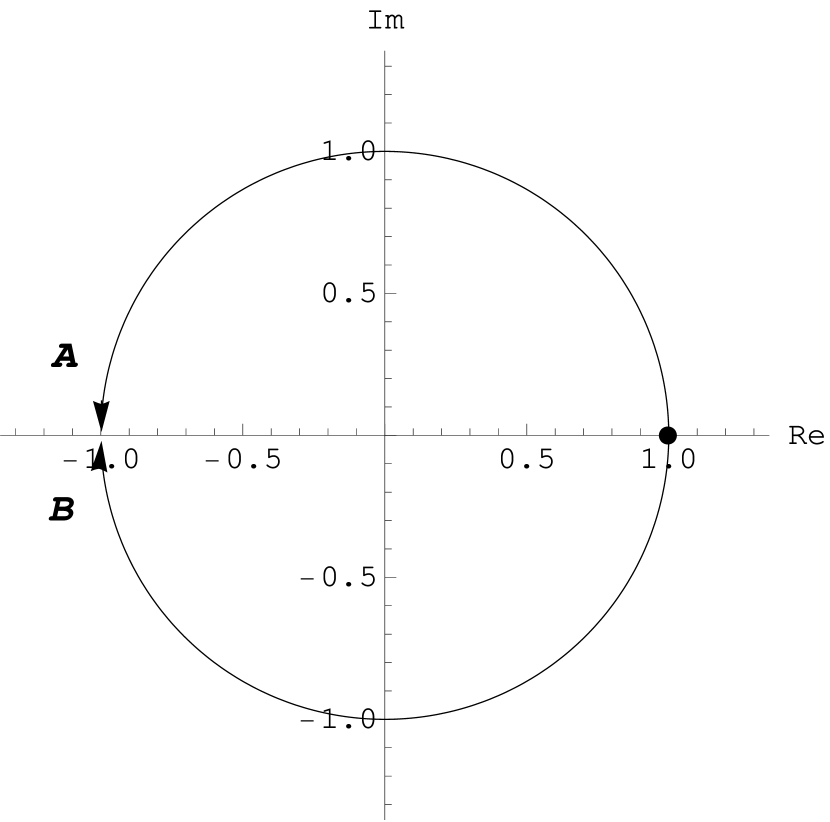
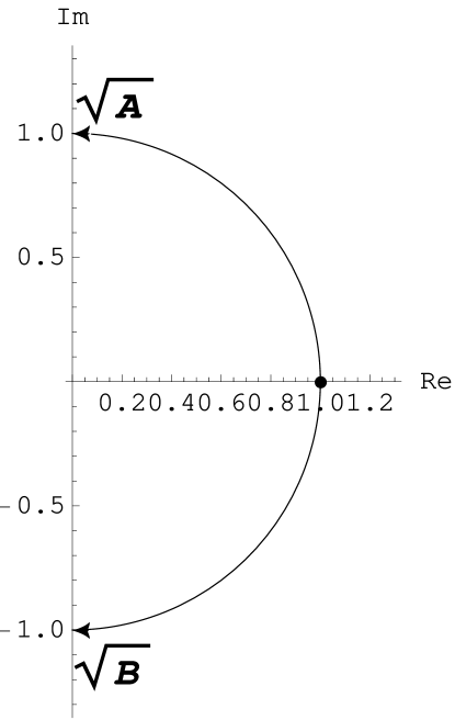
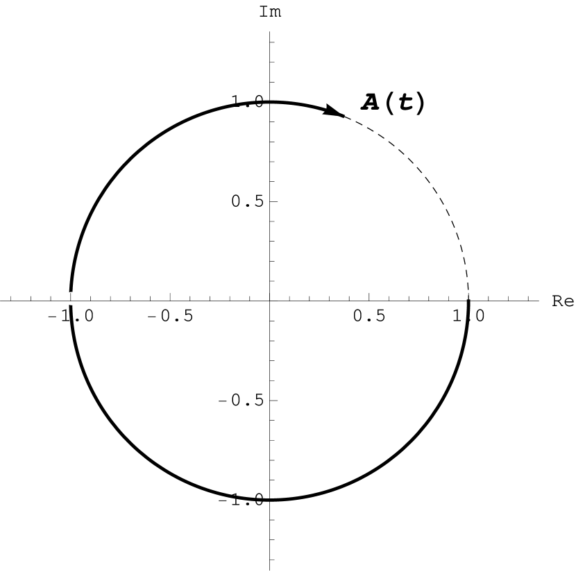
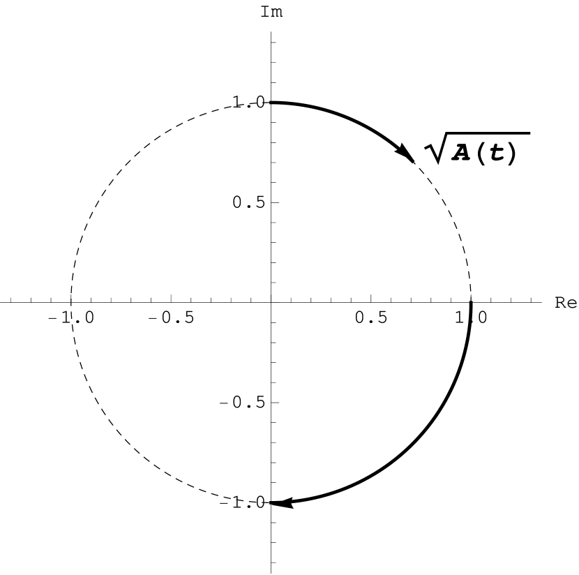
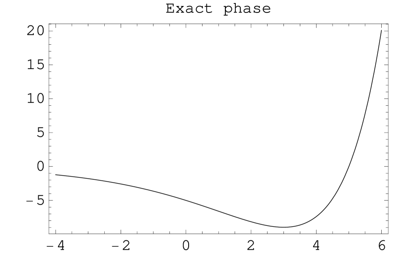
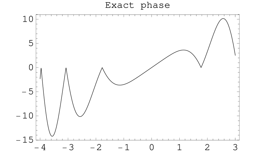
Figure 1: The first two lines of figures illustrate
the complex square root calcutated by MatLab or
Wolfram Mathematica. The complex square root is implemented as a function which is continuous at the positive half line z > 0 𝑧 0 z>0 z < 0 𝑧 0 z<0 ( mod 2 π ) mod 2 𝜋 ({\rm mod}\,2\pi) 54 [19 ] ).
Recall that numerical values of z 𝑧 \sqrt{z}
z = { | z | e i 2 ϕ , if ϕ ∈ [ 0 , π ] ; | z | e i 2 ( ϕ − 2 π ) , if ϕ ∈ ( π , 2 π ) } , \sqrt{z}=\{\sqrt{|z|}e^{\frac{i}{2}\phi},\;{\rm if}\;\phi\in[0,\pi];\;\;\sqrt{|z|}e^{\frac{i}{2}(\phi-2\pi)},\;{\rm if}\;\phi\in(\pi,2\pi)\}, (53)
that is ϕ = π italic-ϕ 𝜋 \phi=\pi [20 ] . At the same time Φ t subscript Φ 𝑡 \sqrt{\Phi_{t}} 3 Φ 0 = I subscript Φ 0 𝐼 \Phi_{0}=I Arg det Φ t Arg subscript Φ 𝑡 \sqrt{{\rm Arg}\det\Phi_{t}} [ 0 , π ] 0 𝜋 [0,\pi] [ − π / 2 , π / 2 ] 𝜋 2 𝜋 2 [-\pi/2,\pi/2] t 𝑡 t
On the other hand, the matrix elements of
e G t = ( Φ t Ψ t Ψ ¯ t Φ ¯ t ) superscript 𝑒 𝐺 𝑡 subscript Φ 𝑡 subscript Ψ 𝑡 subscript ¯ Ψ 𝑡 subscript ¯ Φ 𝑡 e^{Gt}=\left(\begin{array}[]{cc}\Phi_{t}&\Psi_{t}\\
\overline{\Psi}_{t}&\overline{\Phi}_{t}\end{array}\right) 3 52 t 𝑡 t 3 52 tr ρ ¯ τ A trace subscript ¯ 𝜌 𝜏 𝐴 \tr\overline{\rho}_{\tau}A n > 3 𝑛 3 n>3 52 3 s t subscript 𝑠 𝑡 s_{t} index .
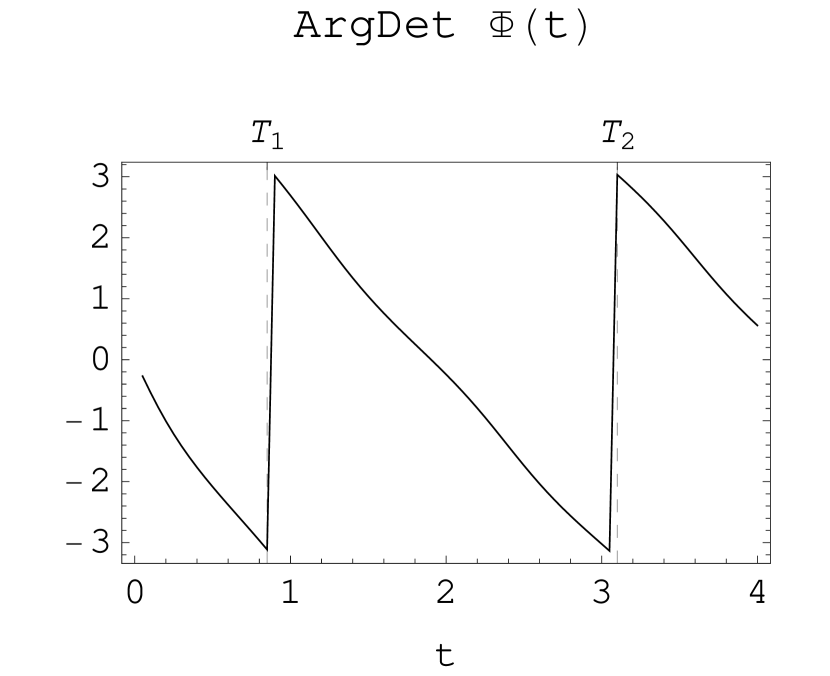
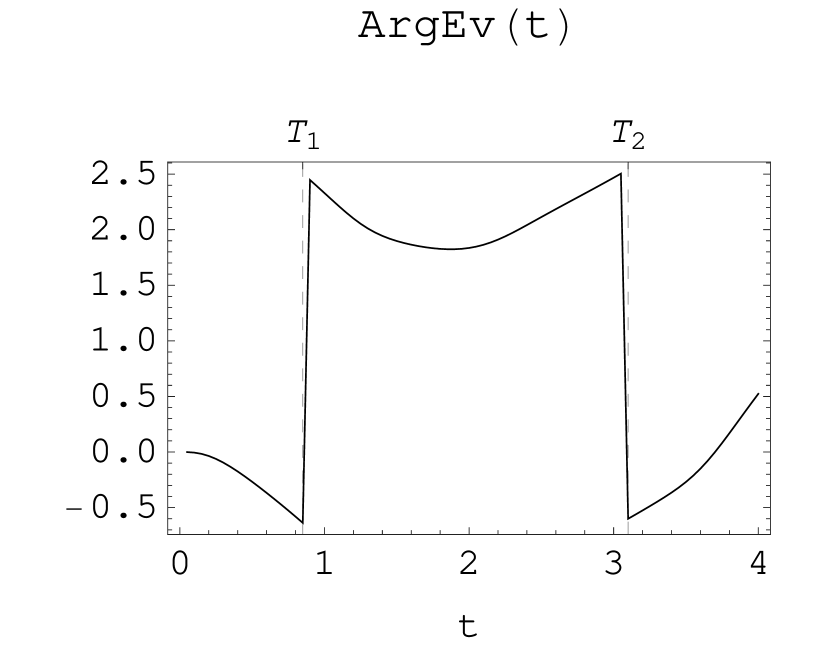
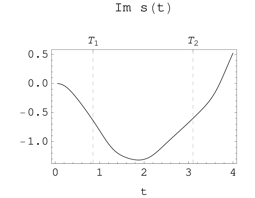
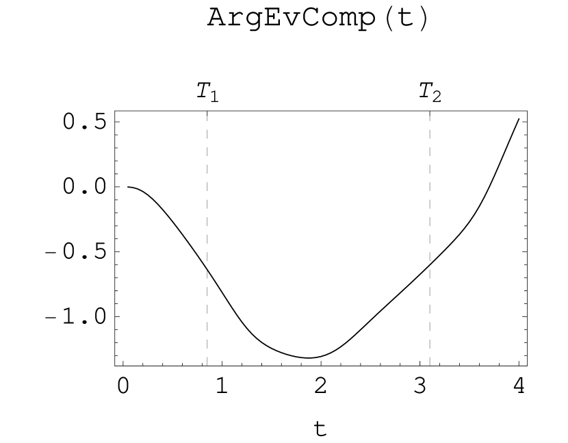
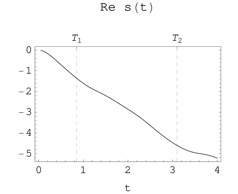
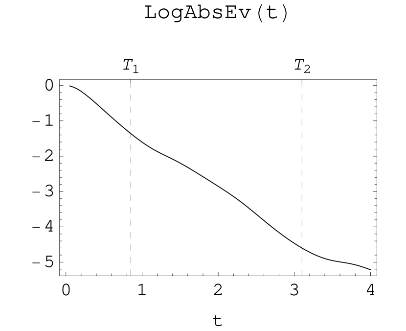
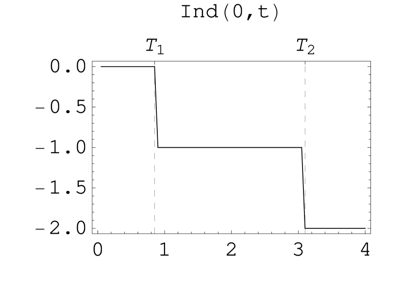
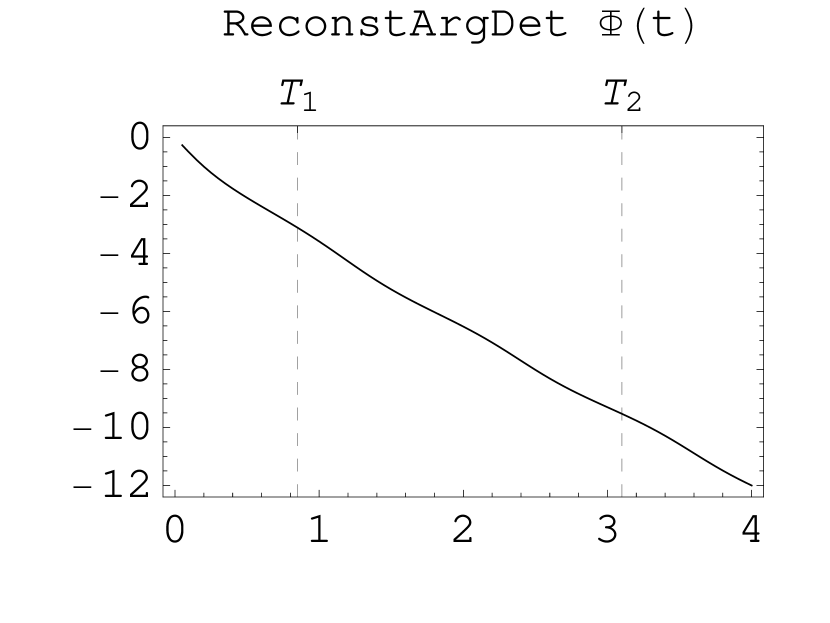
Figure 2: The first two panels show the discontinuous functions
ArgDet Φ t ∈ [ − π , π ] ArgDet subscript Φ 𝑡 𝜋 𝜋 {\rm ArgDet}\,\Phi_{t}\in[-\pi,\pi] Arg e − i t 2 tr B det Φ t ∈ [ − π , π ] Arg superscript 𝑒 𝑖 𝑡 2 trace 𝐵 subscript Φ 𝑡 𝜋 𝜋 {\rm Arg\,}\frac{e^{-\frac{it}{2}\tr B}}{\sqrt{\det\Phi_{t}}}\in[-\pi,\pi] 3 Im s t ∈ ℝ Im subscript 𝑠 𝑡 ℝ {\rm Im}\,s_{t}\in{\mathbb{R}} 46 47 Im S t Im subscript 𝑆 𝑡 {\rm Im}\,S_{t} S t = Arg e − i t 2 tr B + i π Ind ( 0 , t ) det Φ t subscript 𝑆 𝑡 Arg superscript 𝑒 𝑖 𝑡 2 trace 𝐵 𝑖 𝜋 Ind 0 𝑡 subscript Φ 𝑡 S_{t}={\rm Arg}\frac{e^{-\frac{it}{2}\tr B+i\pi\,{\rm Ind}(0,t)}}{\sqrt{\det\Phi_{t}}} i π Ind ( 0 , t ) 𝑖 𝜋 Ind 0 𝑡 i\pi\,{\rm Ind}(0,t) ∫ 0 t 1 2 tr ρ ¯ τ A d τ superscript subscript 0 𝑡 1 2 trace subscript ¯ 𝜌 𝜏 𝐴 𝑑 𝜏 \int_{0}^{t}\frac{1}{2}\,\tr\,\overline{\rho}_{\tau}A\,d\tau 46 Log | e − i t 2 tr B det Φ t | Log superscript 𝑒 𝑖 𝑡 2 trace 𝐵 subscript Φ 𝑡 {\rm Log}|\frac{e^{-\frac{it}{2}\tr B}}{\sqrt{\det\Phi_{t}}}| 3 Ind ( 0 , t ) Ind 0 𝑡 {\rm Ind}(0,t) 54 ArgDet Φ ( t ) ArgDet Φ 𝑡 {\rm ArgDet}\Phi(t)
An analogue of the construction of index introduced by V. P. Maslov for non-degenerate (recall that det | Φ t | ≥ 1 subscript Φ 𝑡 1 \det|\Phi_{t}|\geq 1 Φ t subscript Φ 𝑡 \Phi_{t} Φ t = U t | Φ t | subscript Φ 𝑡 subscript 𝑈 𝑡 subscript Φ 𝑡 \Phi_{t}=U_{t}\,|\Phi_{t}| U s subscript 𝑈 𝑠 U_{s} ( 0 , t ) 0 𝑡 (0,t)
Set φ ( t ) = 1 2 ∑ k λ k ( t ) ∈ ( − π , π ] 𝜑 𝑡 1 2 subscript 𝑘 subscript 𝜆 𝑘 𝑡 𝜋 𝜋 \varphi(t)=\frac{1}{2}\sum_{k}\lambda_{k}(t)\in(-\pi,\pi] λ k ( t ) subscript 𝜆 𝑘 𝑡 \lambda_{k}(t) e i λ k ( t ) superscript 𝑒 𝑖 subscript 𝜆 𝑘 𝑡 e^{i\lambda_{k}(t)} U t subscript 𝑈 𝑡 U_{t} { T k } : 0 < T 1 < T 2 < … < T n ( t ) < t : subscript 𝑇 𝑘 0 subscript 𝑇 1 subscript 𝑇 2 … subscript 𝑇 𝑛 𝑡 𝑡 \{T_{k}\}:\;0<T_{1}<T_{2}<\dots<T_{n(t)}<t 2 π 2 𝜋 2\pi φ ( t ) 𝜑 𝑡 \varphi(t) ( − π , π ] 𝜋 𝜋 (-\pi,\pi] t 𝑡 t φ ( t ) 𝜑 𝑡 \varphi(t) − π 𝜋 -\pi π 𝜋 \pi φ ( t ) 𝜑 𝑡 \varphi(t)
Ind ( s , t ) = def − ∑ T n ∈ ( s , t ) sign ( φ ( T n + 0 ) − φ ( T n − 0 ) ) , superscript def Ind 𝑠 𝑡 subscript subscript 𝑇 𝑛 𝑠 𝑡 sign 𝜑 subscript 𝑇 𝑛 0 𝜑 subscript 𝑇 𝑛 0 {\rm Ind}(s,t)\stackrel{{\scriptstyle\rm def}}{{=}}-\sum_{T_{n}\in(s,t)}{\rm sign}(\varphi(T_{n}+0)-\varphi(T_{n}-0)), (54)
e i H ^ 2 t = e − i t 2 tr B + i π Ind ( 0 , t ) det Φ t e − 1 2 ( a † , R t a † ) : e ( a † , ( Φ t − 1 − I ) a ) : e 1 2 ( a , ρ ¯ t a ) : superscript 𝑒 𝑖 subscript ^ 𝐻 2 𝑡 superscript 𝑒 𝑖 𝑡 2 trace 𝐵 𝑖 𝜋 Ind 0 𝑡 subscript Φ 𝑡 superscript 𝑒 1 2 superscript 𝑎 † subscript 𝑅 𝑡 superscript 𝑎 † superscript 𝑒 superscript 𝑎 † superscript subscript Φ 𝑡 1 𝐼 𝑎 : superscript 𝑒 1 2 𝑎 subscript ¯ 𝜌 𝑡 𝑎 e^{i\widehat{H}_{2}t}=\frac{e^{-\frac{it}{2}\tr B+i\pi{\rm Ind}(0,t)}}{\sqrt{\det\Phi_{t}}}\,e^{-\frac{1}{2}(a^{\dagger},R_{t}a^{\dagger})}\,:e^{(a^{\dagger},(\Phi_{t}^{-1}-I)a)}:\,e^{\frac{1}{2}(a,\overline{\rho}_{t}a)} (55)
is a continuous function, where the square root and the index are calculated according to (53 54
In next section, we derive a pure algebraic representation of s t subscript 𝑠 𝑡 s_{t}
4 Algebraic forms of e s t superscript 𝑒 subscript 𝑠 𝑡 e^{s_{t}}
For z ∈ ℂ n 𝑧 superscript ℂ 𝑛 z\in\mathbb{C}^{n} ψ ( z ) = e ( z , a † ) − ( z ¯ , a ) | 0 ⟩ = | z ⟩ 𝜓 𝑧 superscript 𝑒 𝑧 superscript 𝑎 † ¯ 𝑧 𝑎 ket 0 ket 𝑧 \psi(z)=e^{(z,a^{\dagger})-(\overline{z},a)}|0\rangle=|z\rangle 52 e i H ^ 2 t superscript 𝑒 𝑖 subscript ^ 𝐻 2 𝑡 e^{i\widehat{H}_{2}t}
⟨ z | e i H ^ 2 t | z ⟩ = e i Ind ( 0 , t ) − i t 2 tr B det Φ t e − 1 2 ( z ¯ , R t z ¯ ) e ( z ¯ , ( Φ t − 1 − I ) z ) e 1 2 ( z , ρ ¯ t z ) , quantum-operator-product 𝑧 superscript 𝑒 𝑖 subscript ^ 𝐻 2 𝑡 𝑧 superscript 𝑒 𝑖 Ind 0 𝑡 𝑖 𝑡 2 trace 𝐵 subscript Φ 𝑡 superscript 𝑒 1 2 ¯ 𝑧 subscript 𝑅 𝑡 ¯ 𝑧 superscript 𝑒 ¯ 𝑧 superscript subscript Φ 𝑡 1 𝐼 𝑧 superscript 𝑒 1 2 𝑧 subscript ¯ 𝜌 𝑡 𝑧 \langle z|e^{i\widehat{H}_{2}t}|z\rangle=\frac{e^{i{\rm Ind}(0,t)-\frac{it}{2}\tr B}}{\sqrt{\det\Phi_{t}}}\,e^{-\frac{1}{2}(\overline{z},R_{t}\overline{z})}\,e^{(\overline{z},\bigl{(}\Phi_{t}^{-1}-I\bigr{)}z)}\,e^{\frac{1}{2}(z,\overline{\rho}_{t}z)},
and the commutation rule e − ( a † , z ) + ( a , z ¯ ) F ( a † , a ) e ( a † , z ) − ( a , z ¯ ) = F ( a † + z ¯ , a + z ) superscript 𝑒 superscript 𝑎 † 𝑧 𝑎 ¯ 𝑧 𝐹 superscript 𝑎 † 𝑎 superscript 𝑒 superscript 𝑎 † 𝑧 𝑎 ¯ 𝑧 𝐹 superscript 𝑎 † ¯ 𝑧 𝑎 𝑧 e^{-(a^{\dagger},z)+(a,\overline{z})}F(a^{\dagger},a)e^{(a^{\dagger},z)-(a,\overline{z})}=F(a^{\dagger}+\overline{z},a+z)
e i Ind ( 0 , t ) − i t 2 tr B det Φ t e − 1 2 ( z ¯ , R t z ¯ ) e ( z ¯ , ( Φ t − 1 − I ) z ) e 1 2 ( z , ρ ¯ t z ) = ⟨ z | e i H ^ 2 t | z ⟩ = ⟨ 0 | e i H 2 ( a † + z ¯ , a + z ) t | 0 ⟩ superscript 𝑒 𝑖 Ind 0 𝑡 𝑖 𝑡 2 trace 𝐵 subscript Φ 𝑡 superscript 𝑒 1 2 ¯ 𝑧 subscript 𝑅 𝑡 ¯ 𝑧 superscript 𝑒 ¯ 𝑧 subscript superscript Φ 1 𝑡 𝐼 𝑧 superscript 𝑒 1 2 𝑧 subscript ¯ 𝜌 𝑡 𝑧 quantum-operator-product 𝑧 superscript 𝑒 𝑖 subscript ^ 𝐻 2 𝑡 𝑧 quantum-operator-product 0 superscript 𝑒 𝑖 subscript 𝐻 2 superscript 𝑎 † ¯ 𝑧 𝑎 𝑧 𝑡 0 \displaystyle\frac{e^{i{\rm Ind}(0,t)-\frac{it}{2}\tr B}}{\sqrt{\det\Phi_{t}}}\,e^{-\frac{1}{2}(\overline{z},R_{t}\overline{z})}\,e^{(\overline{z},\bigl{(}\Phi^{-1}_{t}-I\bigr{)}z)}\,e^{\frac{1}{2}(z,\overline{\rho}_{t}z)}=\langle z|e^{i\widehat{H}_{2}t}|z\rangle=\langle 0|e^{iH_{2}(a^{\dagger}+\overline{z},a+z)t}|0\rangle
= ⟨ 0 | e ( i H ^ 2 − ( a † , x ) + ( a , x ¯ ) ) t | 0 ⟩ e i t ( z ¯ , B z ) − 1 2 ( z ¯ , A z ¯ ) + 1 2 ( z , A ¯ z ) = e s t e i t Im ( z , h ¯ ) , absent quantum-operator-product 0 superscript 𝑒 𝑖 subscript ^ 𝐻 2 superscript 𝑎 † 𝑥 𝑎 ¯ 𝑥 𝑡 0 superscript 𝑒 𝑖 𝑡 ¯ 𝑧 𝐵 𝑧 1 2 ¯ 𝑧 𝐴 ¯ 𝑧 1 2 𝑧 ¯ 𝐴 𝑧 superscript 𝑒 subscript 𝑠 𝑡 superscript 𝑒 𝑖 𝑡 Im 𝑧 ¯ ℎ \displaystyle=\langle 0|e^{\bigl{(}i\widehat{H}_{2}-(a^{\dagger},x)+(a,\overline{x})\bigr{)}t}|0\rangle\,e^{it(\overline{z},Bz)-\frac{1}{2}(\overline{z},A\overline{z})+\frac{1}{2}(z,\overline{A}z)}=e^{s_{t}}\,e^{it{\rm Im\,}(z,\overline{h})},
where we set x = A z ¯ − i B z 𝑥 𝐴 ¯ 𝑧 𝑖 𝐵 𝑧 x=A\overline{z}-iBz x ¯ = A ¯ z + i B ¯ z ¯ ¯ 𝑥 ¯ 𝐴 𝑧 𝑖 ¯ 𝐵 ¯ 𝑧 \overline{x}=\overline{A}z+i\overline{B}\overline{z} det G ≠ 0 𝐺 0 \det G\neq 0 A z ¯ − i B z = h 𝐴 ¯ 𝑧 𝑖 𝐵 𝑧 ℎ A\overline{z}-iBz=h A ¯ z + i B ¯ z ¯ = h ¯ ¯ 𝐴 𝑧 𝑖 ¯ 𝐵 ¯ 𝑧 ¯ ℎ \overline{A}z+i\overline{B}\overline{z}=\overline{h} { z , z ¯ } 𝑧 ¯ 𝑧 \{z,\overline{z}\}
( z ( h , h ¯ ) z ¯ ( h , h ¯ ) ) = G − 1 ( h h ¯ ) , H ^ 2 + i ( a † , ( A z ¯ − i B z ) ) − i ( a , ( A ¯ z + i B ¯ z ¯ ) ) | z ( h , h ¯ ) = H ^ . formulae-sequence 𝑧 ℎ ¯ ℎ ¯ 𝑧 ℎ ¯ ℎ superscript 𝐺 1 ℎ ¯ ℎ subscript ^ 𝐻 2 𝑖 superscript 𝑎 † 𝐴 ¯ 𝑧 𝑖 𝐵 𝑧 evaluated-at 𝑖 𝑎 ¯ 𝐴 𝑧 𝑖 ¯ 𝐵 ¯ 𝑧 𝑧 ℎ ¯ ℎ ^ 𝐻 \left(\begin{array}[]{c}z(h,\overline{h})\\
\overline{z}(h,\overline{h})\end{array}\right)=G^{-1}\left(\begin{array}[]{c}h\\
\overline{h}\end{array}\right),\quad\widehat{H}_{2}+i(a^{\dagger},(A\overline{z}-iBz))-i(a,(\overline{A}z+i\overline{B}\overline{z}))|_{z(h,\overline{h})}=\widehat{H}. (56)
Taking into account (2 3 56 det G ≠ 0 det 𝐺 0 {\rm det}\,G\neq 0 e s t superscript 𝑒 subscript 𝑠 𝑡 e^{s_{t}}
e s t = ⟨ 0 | e i H ^ t | 0 ⟩ = e − i t 2 tr B + Q t det Φ t , superscript 𝑒 subscript 𝑠 𝑡 quantum-operator-product 0 superscript 𝑒 𝑖 ^ 𝐻 𝑡 0 superscript 𝑒 𝑖 𝑡 2 trace 𝐵 subscript 𝑄 𝑡 subscript Φ 𝑡 \displaystyle e^{s_{t}}=\langle 0|e^{i\widehat{H}t}|0\rangle=\frac{e^{-\frac{it}{2}\tr B+Q_{t}}}{\sqrt{\det\Phi_{t}}}, (57)
Q t = i Ind ( 0 , t ) + 1 2 ( z , ( ρ ¯ t − A ¯ t ) z ) − 1 2 ( z ¯ , ( R t − A t ) z ¯ ) + ( z ¯ , ( Φ t − 1 − I − i B t ) z ) | z ( h , h ¯ ) . subscript 𝑄 𝑡 𝑖 Ind 0 𝑡 1 2 𝑧 subscript ¯ 𝜌 𝑡 ¯ 𝐴 𝑡 𝑧 1 2 ¯ 𝑧 subscript 𝑅 𝑡 𝐴 𝑡 ¯ 𝑧 evaluated-at ¯ 𝑧 subscript superscript Φ 1 𝑡 𝐼 𝑖 𝐵 𝑡 𝑧 𝑧 ℎ ¯ ℎ \displaystyle Q_{t}=i{\rm Ind}(0,t)+\frac{1}{2}(z,(\overline{\rho}_{t}-\overline{A}t)z)-\frac{1}{2}(\overline{z},(R_{t}-At)\overline{z})+(\overline{z},(\Phi^{-1}_{t}-I-iBt)z)|_{z(h,\overline{h})}.
Note that the second exponential can be represented as a symmetric quadratic form in terms of algebraic operations:
Q t = 1 2 ( G − 1 ( h h ¯ ) , ( ρ ¯ t − A ¯ t ( Φ t T ) − 1 − I − i B ¯ t ( Φ t ) − 1 − I − i B t − R t + A t ) G − 1 ( h h ¯ ) ) . subscript 𝑄 𝑡 1 2 superscript 𝐺 1 ℎ ¯ ℎ subscript ¯ 𝜌 𝑡 ¯ 𝐴 𝑡 superscript superscript subscript Φ 𝑡 𝑇 1 𝐼 𝑖 ¯ 𝐵 𝑡 superscript subscript Φ 𝑡 1 𝐼 𝑖 𝐵 𝑡 subscript 𝑅 𝑡 𝐴 𝑡 superscript 𝐺 1 ℎ ¯ ℎ \displaystyle Q_{t}=\frac{1}{2}\left(G^{-1}\left(\begin{array}[]{c}h\\
\overline{h}\end{array}\right),\left(\begin{array}[]{cc}\overline{\rho}_{t}-\overline{A}t&(\Phi_{t}^{T})^{-1}-I-i\,\overline{B}t\\
(\Phi_{t})^{-1}-I-iBt&-R_{t}+At\end{array}\right)G^{-1}\left(\begin{array}[]{c}h\\
\overline{h}\end{array}\right)\right).
The final result of this section is an algebraic representation of s t subscript 𝑠 𝑡 s_{t} e G t superscript 𝑒 𝐺 𝑡 e^{Gt} G − 1 ( e G t − I ) superscript 𝐺 1 superscript 𝑒 𝐺 𝑡 𝐼 G^{-1}(e^{Gt}-I) G − 2 ( e G t − I − G t ) superscript 𝐺 2 superscript 𝑒 𝐺 𝑡 𝐼 𝐺 𝑡 G^{-2}(e^{Gt}-I-Gt) G 𝐺 G
For H ^ = H ^ 2 − ( a † , h ) + ( a , h ¯ ) ^ 𝐻 subscript ^ 𝐻 2 superscript 𝑎 † ℎ 𝑎 ¯ ℎ \widehat{H}=\widehat{H}_{2}-(a^{\dagger},h)+(a,\overline{h}) e s t = ⟨ 0 | e i H ^ t | 0 ⟩ = ⟨ ϕ t | e − i H ^ 2 t e i H ^ t | 0 ⟩ superscript 𝑒 subscript 𝑠 𝑡 quantum-operator-product 0 superscript 𝑒 𝑖 ^ 𝐻 𝑡 0 quantum-operator-product subscript italic-ϕ 𝑡 superscript 𝑒 𝑖 subscript ^ 𝐻 2 𝑡 superscript 𝑒 𝑖 ^ 𝐻 𝑡 0 e^{s_{t}}=\langle 0|e^{i\widehat{H}t}|0\rangle=\langle\phi_{t}|e^{-i\widehat{H}_{2}t}e^{i\widehat{H}t}|0\rangle ϕ t = def e − i H ^ 2 t | 0 ⟩ ∈ ⊗ 1 n ℓ 2 \phi_{t}\stackrel{{\scriptstyle\rm def}}{{=}}e^{-i\widehat{H}_{2}t}|0\rangle\in\otimes_{1}^{n}\ell_{2} ⊗ 1 n ℓ 2 superscript subscript tensor-product 1 𝑛 absent subscript ℓ 2 \otimes_{1}^{n}\ell_{2} ℒ 2 ( ℝ n ) subscript ℒ 2 superscript ℝ 𝑛 {\mathcal{L}}_{2}({\mathbb{R}}^{n})
⊗ 1 n ℓ 2 ∋ | 0 ⟩ ↔ e − 1 2 | x | 2 π n 4 ∈ ℒ 2 ( ℝ n ) , a ↔ x + ∂ x 2 , a † ↔ x − ∂ x 2 , \otimes_{1}^{n}\ell_{2}\ni|0\rangle\leftrightarrow\frac{e^{-\frac{1}{2}|x|^{2}}}{\pi^{\frac{n}{4}}}\in{\mathcal{L}}_{2}({\mathbb{R}}^{n}),\quad a\leftrightarrow\frac{x+\partial_{x}}{\sqrt{2}},\quad a^{\dagger}\leftrightarrow\frac{x-\partial_{x}}{\sqrt{2}},
decomposition (39
e − i H ^ 2 t | 0 ⟩ = e i Ind ( 0 , t ) + i t 2 tr B det Φ − t e − 1 2 ( a † , R − t a † ) | 0 ⟩ ↔ e i Ind ( 0 , t ) + | x | 2 2 − ( x , ( I − R − t ) − 1 x ) π n 4 det Φ − t det ( I − R − t ) = def ϕ t ( x ) ↔ superscript 𝑒 𝑖 subscript ^ 𝐻 2 𝑡 ket 0 superscript 𝑒 𝑖 Ind 0 𝑡 𝑖 𝑡 2 trace 𝐵 subscript Φ 𝑡 superscript 𝑒 1 2 superscript 𝑎 † subscript 𝑅 𝑡 superscript 𝑎 † ket 0 superscript def superscript 𝑒 𝑖 Ind 0 𝑡 superscript 𝑥 2 2 𝑥 superscript 𝐼 subscript 𝑅 𝑡 1 𝑥 superscript 𝜋 𝑛 4 subscript Φ 𝑡 𝐼 subscript 𝑅 𝑡 subscript italic-ϕ 𝑡 𝑥 \displaystyle e^{-i\widehat{H}_{2}t}|0\rangle=\frac{e^{i{\rm Ind}(0,t)+\frac{it}{2}\tr B}}{\sqrt{\det\Phi_{-t}}}\,e^{-\frac{1}{2}(a^{\dagger},R_{-t}a^{\dagger})}|0\rangle\leftrightarrow\frac{e^{i{\rm Ind}(0,t)+\frac{|x|^{2}}{2}-(x,(I-R_{-t})^{-1}x)}}{\pi^{\frac{n}{4}}\sqrt{\det\Phi_{-t}\det(I-R_{-t})}}\stackrel{{\scriptstyle\rm def}}{{=}}\phi_{t}(x)
= e i Ind ( 0 , t ) + | x | 2 2 − ( x , ( I + ρ t ) − 1 x ) π n 4 det Φ t det ( I + ρ t ) = def ϕ t ( x ) , absent superscript 𝑒 𝑖 Ind 0 𝑡 superscript 𝑥 2 2 𝑥 superscript 𝐼 subscript 𝜌 𝑡 1 𝑥 superscript 𝜋 𝑛 4 subscript Φ 𝑡 𝐼 subscript 𝜌 𝑡 superscript def subscript italic-ϕ 𝑡 𝑥 \displaystyle=\frac{e^{i{\rm Ind}(0,t)+\frac{|x|^{2}}{2}-(x,(I+\rho_{t})^{-1}x)}}{\pi^{\frac{n}{4}}\sqrt{\det\Phi_{t}\det(I+\rho_{t})}}\stackrel{{\scriptstyle\rm def}}{{=}}\phi_{t}(x), (59)
where ϕ t ( x ) ∈ ℒ 2 ( ℝ n ) subscript italic-ϕ 𝑡 𝑥 subscript ℒ 2 superscript ℝ 𝑛 \phi_{t}(x)\in{\mathcal{L}}_{2}({\mathbb{R}}^{n}) R − t = − ρ t subscript 𝑅 𝑡 subscript 𝜌 𝑡 R_{-t}=-\rho_{t} Φ − t = Φ t ∗ subscript Φ 𝑡 subscript superscript Φ 𝑡 \Phi_{-t}=\Phi^{*}_{t} 32 det Φ t det Φ ¯ t det ( I − R t R t ¯ ) = 1 subscript Φ 𝑡 subscript ¯ Φ 𝑡 𝐼 subscript 𝑅 𝑡 ¯ subscript 𝑅 𝑡 1 \det\Phi_{t}\,\det\overline{\Phi}_{t}\,\det(I-R_{t}\overline{R_{t}})=1
det Φ t det Φ ¯ t det ( I − R t ) det ( I − R t ¯ ) det ( ( I − R t ) − 1 + ( I − R ¯ t ) − 1 − I ) = 1 . subscript Φ 𝑡 subscript ¯ Φ 𝑡 𝐼 subscript 𝑅 𝑡 𝐼 ¯ subscript 𝑅 𝑡 superscript 𝐼 subscript 𝑅 𝑡 1 superscript 𝐼 subscript ¯ 𝑅 𝑡 1 𝐼 1 \displaystyle\det\Phi_{t}\,\det\overline{\Phi}_{t}\,\det(I-R_{t})\,\det(I-\overline{R_{t}})\det\biggl{(}(I-R_{t})^{-1}+(I-\overline{R}_{t})^{-1}-I\biggr{)}=1. (60)
Let us prove the unitary equivalence of exponential vectors from ℓ 2 subscript ℓ 2 \ell_{2} ℒ 2 subscript ℒ 2 {\mathcal{L}}_{2}
ψ t = e − i H ^ 2 t e i ( H ^ 2 − ( a † , h ) + ( a , h ¯ ) ) t | 0 ⟩ = e − ( a † , h t ) + i γ t − | h t | 2 2 | 0 ⟩ ↔ ↔ subscript 𝜓 𝑡 superscript 𝑒 𝑖 subscript ^ 𝐻 2 𝑡 superscript 𝑒 𝑖 subscript ^ 𝐻 2 superscript 𝑎 † ℎ 𝑎 ¯ ℎ 𝑡 ket 0 superscript 𝑒 superscript 𝑎 † subscript ℎ 𝑡 𝑖 subscript 𝛾 𝑡 superscript subscript ℎ 𝑡 2 2 ket 0 absent \displaystyle\psi_{t}=e^{-i\widehat{H}_{2}t}e^{i(\widehat{H}_{2}-(a^{\dagger},h)+(a,\overline{h}))t}|0\rangle=e^{-(a^{\dagger},h_{t})+i\gamma_{t}-\frac{|h_{t}|^{2}}{2}}|0\rangle\leftrightarrow
↔ e i γ t − ( h t , h ¯ t − h t ) 2 π n 4 e − 1 2 ( x + 2 h t , x + 2 h t ) = def ψ t ( x ) , ↔ absent superscript def superscript 𝑒 𝑖 subscript 𝛾 𝑡 subscript ℎ 𝑡 subscript ¯ ℎ 𝑡 subscript ℎ 𝑡 2 superscript 𝜋 𝑛 4 superscript 𝑒 1 2 𝑥 2 subscript ℎ 𝑡 𝑥 2 subscript ℎ 𝑡 subscript 𝜓 𝑡 𝑥 \displaystyle\leftrightarrow\frac{e^{i\gamma_{t}-\frac{(h_{t},\overline{h}_{t}-h_{t})}{2}}}{\pi^{\frac{n}{4}}}e^{-\frac{1}{2}(x+\sqrt{2}h_{t},x+\sqrt{2}h_{t})}\stackrel{{\scriptstyle\rm def}}{{=}}\psi_{t}(x), (61)
where h t subscript ℎ 𝑡 h_{t} h ¯ t subscript ¯ ℎ 𝑡 \overline{h}_{t} 31
γ t = Im ∫ 0 t ( h ˙ s , h ¯ s ) 𝑑 s , e s t = ⟨ ϕ t , ψ t ⟩ l 2 = ∫ ℝ n ϕ ¯ t ( x ) ψ t ( x ) d n x = ∫ ℝ n ϕ − t ( x ) ψ t ( x ) d n x . formulae-sequence subscript 𝛾 𝑡 Im superscript subscript 0 𝑡 subscript ˙ ℎ 𝑠 subscript ¯ ℎ 𝑠 differential-d 𝑠 superscript 𝑒 subscript 𝑠 𝑡 subscript subscript italic-ϕ 𝑡 subscript 𝜓 𝑡
subscript 𝑙 2 subscript superscript ℝ 𝑛 subscript ¯ italic-ϕ 𝑡 𝑥 subscript 𝜓 𝑡 𝑥 superscript 𝑑 𝑛 𝑥 subscript superscript ℝ 𝑛 subscript italic-ϕ 𝑡 𝑥 subscript 𝜓 𝑡 𝑥 superscript 𝑑 𝑛 𝑥 \displaystyle\gamma_{t}={\rm Im\,}\int_{0}^{t}(\dot{h}_{s},{\overline{h}_{s}})ds,\;e^{s_{t}}=\langle\phi_{t},\psi_{t}\rangle_{l_{2}}=\int_{{\mathbb{R}}^{n}}\overline{\phi}_{t}(x)\psi_{t}(x)d^{n}x=\int_{{\mathbb{R}}^{n}}\phi_{-t}(x)\psi_{t}(x)d^{n}x. (62)
By taking the time derivative of the left hand side of (61 ℓ 2 subscript ℓ 2 \ell_{2}
( Φ − t a + Ψ − t a † , h ¯ ) − ( Φ ¯ − t a † + Ψ ¯ − t a , h ) − ( a + h t , h ¯ t ˙ ) + ( a † , h ˙ t ) + i γ ˙ t − ( h t , h ¯ t ˙ ) − ( h ˙ t , h ¯ t ) 2 = 0 . subscript Φ 𝑡 𝑎 subscript Ψ 𝑡 superscript 𝑎 † ¯ ℎ subscript ¯ Φ 𝑡 superscript 𝑎 † subscript ¯ Ψ 𝑡 𝑎 ℎ 𝑎 subscript ℎ 𝑡 ˙ subscript ¯ ℎ 𝑡 superscript 𝑎 † subscript ˙ ℎ 𝑡 𝑖 subscript ˙ 𝛾 𝑡 subscript ℎ 𝑡 ˙ subscript ¯ ℎ 𝑡 subscript ˙ ℎ 𝑡 subscript ¯ ℎ 𝑡 2 0 \displaystyle(\Phi_{-t}a+\Psi_{-t}a^{\dagger},\overline{h})-(\overline{\Phi}_{-t}a^{\dagger}+\overline{\Psi}_{-t}a,h)-(a+h_{t},\dot{\overline{h}_{t}})+(a^{\dagger},\dot{h}_{t})+i\dot{\gamma}_{t}-\frac{(h_{t},\dot{\overline{h}_{t}})-(\dot{h}_{t},{\overline{h}_{t}})}{2}=0.
Note that zero values of coefficients at a 𝑎 a a † superscript 𝑎 † a^{\dagger} I 𝐼 I Φ − t = Φ t ∗ subscript Φ 𝑡 superscript subscript Φ 𝑡 \Phi_{-t}=\Phi_{t}^{*} Ψ − t = − Ψ t T subscript Ψ 𝑡 superscript subscript Ψ 𝑡 𝑇 \Psi_{-t}=-\Psi_{t}^{T}
( h ˙ t h ¯ t ˙ ) = ( Φ t Ψ t Ψ ¯ t Φ ¯ t ) ( h t h ¯ t ) , i γ ˙ t = ( h ˙ t , h ¯ t ) − ( h t , h ¯ t ˙ ) 2 = i Im ( h ˙ t , h ¯ t ) . formulae-sequence subscript ˙ ℎ 𝑡 ˙ subscript ¯ ℎ 𝑡 subscript Φ 𝑡 subscript Ψ 𝑡 subscript ¯ Ψ 𝑡 subscript ¯ Φ 𝑡 subscript ℎ 𝑡 subscript ¯ ℎ 𝑡 𝑖 subscript ˙ 𝛾 𝑡 subscript ˙ ℎ 𝑡 subscript ¯ ℎ 𝑡 subscript ℎ 𝑡 ˙ subscript ¯ ℎ 𝑡 2 𝑖 Im subscript ˙ ℎ 𝑡 subscript ¯ ℎ 𝑡 \displaystyle\left(\begin{array}[]{c}\dot{h}_{t}\\
\dot{\overline{h}_{t}}\end{array}\right)=\left(\begin{array}[]{cc}\Phi_{t}&\Psi_{t}\\
\overline{\Psi}_{t}&\overline{\Phi}_{t}\end{array}\right)\left(\begin{array}[]{c}h_{t}\\
\overline{h}_{t}\end{array}\right),\quad i\dot{\gamma}_{t}=\frac{(\dot{h}_{t},\overline{h}_{t})-(h_{t},\dot{\overline{h}_{t}})}{2}=i{\rm Im\,}(\dot{h}_{t},\overline{h}_{t}).
Consider the integral representation of (62
( h t h ¯ t ) = e G t − I G ( h h ¯ ) , i γ t = i Im ∫ 0 t ( h ˙ s , h ¯ s ) 𝑑 s = 1 2 ∫ 0 t det ( h ˙ t h ˙ ¯ t h t h ¯ t ) d s formulae-sequence subscript ℎ 𝑡 subscript ¯ ℎ 𝑡 superscript 𝑒 𝐺 𝑡 𝐼 𝐺 ℎ ¯ ℎ 𝑖 subscript 𝛾 𝑡 𝑖 Im superscript subscript 0 𝑡 subscript ˙ ℎ 𝑠 subscript ¯ ℎ 𝑠 differential-d 𝑠 1 2 superscript subscript 0 𝑡 subscript ˙ ℎ 𝑡 subscript ¯ ˙ ℎ 𝑡 subscript ℎ 𝑡 subscript ¯ ℎ 𝑡 𝑑 𝑠 \displaystyle\left(\begin{array}[]{c}h_{t}\\
{\overline{h}_{t}}\end{array}\right)=\frac{e^{Gt}-I}{G}\left(\begin{array}[]{c}h\\
{\overline{h}}\end{array}\right),\quad i\gamma_{t}=i{\rm Im\,}\int_{0}^{t}(\dot{h}_{s},\overline{h}_{s})ds=\frac{1}{2}\int_{0}^{t}\det\left(\begin{array}[]{cc}\dot{h}_{t}&{\overline{\dot{h}}}_{t}\\
h_{t}&\overline{h}_{t}\end{array}\right)ds
and let us transform the above integral to algebraic form:
i γ t = 1 2 ( I − G t − e − G t G 2 ( h h ¯ ) , ( h ¯ − h ) ) , e G t ≡ ( Φ t Ψ t Ψ ¯ t Φ ¯ t ) . formulae-sequence 𝑖 subscript 𝛾 𝑡 1 2 𝐼 𝐺 𝑡 superscript 𝑒 𝐺 𝑡 superscript 𝐺 2 ℎ ¯ ℎ ¯ ℎ ℎ superscript 𝑒 𝐺 𝑡 subscript Φ 𝑡 subscript Ψ 𝑡 subscript ¯ Ψ 𝑡 subscript ¯ Φ 𝑡 \displaystyle i\gamma_{t}=\frac{1}{2}\left(\frac{I-Gt-e^{-Gt}}{G^{2}}\,\left(\begin{array}[]{c}h\\
\overline{h}\end{array}\right),\left(\begin{array}[]{c}\overline{h}\\
-h\end{array}\right)\right),\quad e^{Gt}\equiv\left(\begin{array}[]{cc}\Phi_{t}&\Psi_{t}\\
\overline{\Psi}_{t}&\overline{\Phi}_{t}\end{array}\right). (71)
The symplectic property of canonical transformations (18
( Φ t Ψ t Ψ ¯ t Φ ¯ t ) T ( 0 I − I 0 ) ( Φ t Ψ t Ψ ¯ t Φ ¯ t ) = ( Φ t T Ψ t ∗ Ψ t T Φ t ∗ ) ( Ψ ¯ t Φ ¯ t − Φ t − Ψ t ) = ( 0 I − I 0 ) , superscript subscript Φ 𝑡 subscript Ψ 𝑡 subscript ¯ Ψ 𝑡 subscript ¯ Φ 𝑡 𝑇 0 𝐼 𝐼 0 subscript Φ 𝑡 subscript Ψ 𝑡 subscript ¯ Ψ 𝑡 subscript ¯ Φ 𝑡 superscript subscript Φ 𝑡 𝑇 superscript subscript Ψ 𝑡 superscript subscript Ψ 𝑡 𝑇 superscript subscript Φ 𝑡 subscript ¯ Ψ 𝑡 subscript ¯ Φ 𝑡 subscript Φ 𝑡 subscript Ψ 𝑡 0 𝐼 𝐼 0 \displaystyle\left(\begin{array}[]{cc}\Phi_{t}&\Psi_{t}\\
\overline{\Psi}_{t}&\overline{\Phi}_{t}\end{array}\right)^{T}\,\left(\begin{array}[]{cc}0&I\\
-I&0\end{array}\right)\,\left(\begin{array}[]{cc}\Phi_{t}&\Psi_{t}\\
\overline{\Psi}_{t}&\overline{\Phi}_{t}\end{array}\right)=\left(\begin{array}[]{cc}\Phi_{t}^{T}&\Psi_{t}^{*}\\
\Psi_{t}^{T}&\Phi_{t}^{*}\end{array}\right)\,\left(\begin{array}[]{cc}\overline{\Psi}_{t}&\overline{\Phi}_{t}\\
-\Phi_{t}&-\Psi_{t}\end{array}\right)=\left(\begin{array}[]{cc}0&I\\
-I&0\end{array}\right),
( 0 I − I 0 ) e G t = ( 0 I − I 0 ) ( Φ t Ψ t Ψ ¯ t Φ ¯ t ) = ( Φ − t T Ψ − t ∗ Ψ − t T Φ − t ∗ ) ( 0 I − I 0 ) = e − G T t ( 0 I − I 0 ) . 0 𝐼 𝐼 0 superscript 𝑒 𝐺 𝑡 0 𝐼 𝐼 0 subscript Φ 𝑡 subscript Ψ 𝑡 subscript ¯ Ψ 𝑡 subscript ¯ Φ 𝑡 superscript subscript Φ 𝑡 𝑇 superscript subscript Ψ 𝑡 superscript subscript Ψ 𝑡 𝑇 superscript subscript Φ 𝑡 0 𝐼 𝐼 0 superscript 𝑒 superscript 𝐺 𝑇 𝑡 0 𝐼 𝐼 0 \displaystyle\left(\begin{array}[]{cc}0&I\\
-I&0\end{array}\right)\,e^{Gt}=\left(\begin{array}[]{cc}0&I\\
-I&0\end{array}\right)\,\left(\begin{array}[]{cc}\Phi_{t}&\Psi_{t}\\
\overline{\Psi}_{t}&\overline{\Phi}_{t}\end{array}\right)=\left(\begin{array}[]{cc}\Phi_{-t}^{T}&\Psi_{-t}^{*}\\
\Psi_{-t}^{T}&\Phi_{-t}^{*}\end{array}\right)\,\left(\begin{array}[]{cc}0&I\\
-I&0\end{array}\right)=e^{-G^{T}t}\,\left(\begin{array}[]{cc}0&I\\
-I&0\end{array}\right).
Hence from equation (31
2 Im ( h s , h ¯ s ˙ ) = det ( h s h ˙ s h ¯ s h ¯ s ˙ ) = ( e G t − I G ( h h ¯ ) , ( 0 I − I 0 ) e G t ( h h ¯ ) ) = 2 Im subscript ℎ 𝑠 ˙ subscript ¯ ℎ 𝑠 subscript ℎ 𝑠 subscript ˙ ℎ 𝑠 subscript ¯ ℎ 𝑠 ˙ subscript ¯ ℎ 𝑠 superscript 𝑒 𝐺 𝑡 𝐼 𝐺 ℎ ¯ ℎ 0 𝐼 𝐼 0 superscript 𝑒 𝐺 𝑡 ℎ ¯ ℎ absent \displaystyle 2\,{\rm Im\,}(h_{s},\dot{\overline{h}_{s}})=\det\left(\begin{array}[]{cc}h_{s}&\dot{h}_{s}\\
\overline{h}_{s}&\dot{\overline{h}_{s}}\end{array}\right)=\left(\frac{e^{Gt}-I}{G}\,\left(\begin{array}[]{c}h\\
\overline{h}\end{array}\right),\,\left(\begin{array}[]{cc}0&I\\
-I&0\end{array}\right)\,e^{Gt}\left(\begin{array}[]{c}h\\
\overline{h}\end{array}\right)\right)=
( e G t − I G ( h h ¯ ) , e − G T t ( 0 I − I 0 ) ( h h ¯ ) ) = ( I − e − G t G ( h h ¯ ) , ( h ¯ − h ) ) . superscript 𝑒 𝐺 𝑡 𝐼 𝐺 ℎ ¯ ℎ superscript 𝑒 superscript 𝐺 𝑇 𝑡 0 𝐼 𝐼 0 ℎ ¯ ℎ 𝐼 superscript 𝑒 𝐺 𝑡 𝐺 ℎ ¯ ℎ ¯ ℎ ℎ \displaystyle\left(\frac{e^{Gt}-I}{G}\,\left(\begin{array}[]{c}h\\
\overline{h}\end{array}\right),\,e^{-G^{T}t}\left(\begin{array}[]{cc}0&I\\
-I&0\end{array}\right)\,\left(\begin{array}[]{c}h\\
\overline{h}\end{array}\right)\right)=\left(\frac{I-e^{-Gt}}{G}\,\left(\begin{array}[]{c}h\\
\overline{h}\end{array}\right),\,\left(\begin{array}[]{c}\overline{h}\\
-h\end{array}\right)\right).
Integration of this equality in s 𝑠 s [ 0 , t ] 0 𝑡 [0,t] 71 59 61 e s t = ⟨ 0 | e i H ^ t | 0 ⟩ superscript 𝑒 subscript 𝑠 𝑡 quantum-operator-product 0 superscript 𝑒 𝑖 subscript ^ 𝐻 𝑡 0 e^{s_{t}}=\langle 0|e^{i\widehat{H}_{t}}|0\rangle ψ z = e S t − 1 2 ( a † , R t a † ) − ( G t , a † ) | z ⟩ subscript 𝜓 𝑧 superscript 𝑒 subscript 𝑆 𝑡 1 2 superscript 𝑎 † subscript 𝑅 𝑡 superscript 𝑎 † subscript 𝐺 𝑡 superscript 𝑎 † ket 𝑧 \psi_{z}=e^{S_{t}-\frac{1}{2}(a^{\dagger},R_{t}a^{\dagger})-(G_{t},a^{\dagger})}|z\rangle N A , B , h ( z ¯ , z ) = ⟨ z | ψ z ⟩ subscript 𝑁 𝐴 𝐵 ℎ
¯ 𝑧 𝑧 inner-product 𝑧 subscript 𝜓 𝑧 N_{A,B,h}(\overline{z},z)=\langle z|\psi_{z}\rangle
Theorem 2 .
1.
For abitrary symmetric matrix A 𝐴 A , Hermitian matrix B 𝐵 B , and complex vector h ℎ h , the vacuum expectation of the unitary group e i t H ^ superscript 𝑒 𝑖 𝑡 ^ 𝐻 e^{it\widehat{H}} ( 2 ) is equal to
e s t = ⟨ 0 | e i t H ^ | 0 ⟩ = e i Ind ( 0 , t ) + i γ t − 1 2 ( h t , h t ) − 1 2 ( h t , ( h ¯ t − h t ) ) ∫ d n x e − 2 ( h t , x ) − ( x , ( I + ρ t ∗ ) − 1 x ) π n / 4 det ( I + ρ t ∗ ) det Φ t superscript 𝑒 subscript 𝑠 𝑡 quantum-operator-product 0 superscript 𝑒 𝑖 𝑡 ^ 𝐻 0 superscript 𝑒 𝑖 Ind 0 𝑡 𝑖 subscript 𝛾 𝑡 1 2 subscript ℎ 𝑡 subscript ℎ 𝑡 1 2 subscript ℎ 𝑡 subscript ¯ ℎ 𝑡 subscript ℎ 𝑡 superscript 𝑑 𝑛 𝑥 superscript 𝑒 2 subscript ℎ 𝑡 𝑥 𝑥 superscript 𝐼 superscript subscript 𝜌 𝑡 1 𝑥 superscript 𝜋 𝑛 4 𝐼 subscript superscript 𝜌 𝑡 subscript Φ 𝑡 \displaystyle e^{s_{t}}=\langle 0|e^{it\widehat{H}}|0\rangle=e^{i{\rm Ind}(0,t)+i\gamma_{t}-\frac{1}{2}\,(h_{t},h_{t})-\frac{1}{2}\,(h_{t},(\overline{h}_{t}-h_{t}))}\int d^{n}x\frac{e^{-\sqrt{2}(h_{t},x)-(x,(I+\rho_{t}^{*})^{-1}x)}}{\pi^{n/4}\sqrt{\det(I+\rho^{*}_{t})\det\Phi_{t}}}
= e i Ind ( 0 , t ) + i γ t − 1 2 ( ( h t , ( h ¯ t − ρ ¯ t h t ) ) + i t tr B ) det Φ t = e i Ind ( 0 , t ) + i γ t − i t 2 tr B − 1 2 ( h ¯ − t , Φ t − 1 h t ) det Φ t , absent superscript 𝑒 𝑖 Ind 0 𝑡 𝑖 subscript 𝛾 𝑡 1 2 subscript ℎ 𝑡 subscript ¯ ℎ 𝑡 subscript ¯ 𝜌 𝑡 subscript ℎ 𝑡 𝑖 𝑡 trace 𝐵 subscript Φ 𝑡 superscript 𝑒 𝑖 Ind 0 𝑡 𝑖 subscript 𝛾 𝑡 𝑖 𝑡 2 trace 𝐵 1 2 subscript ¯ ℎ 𝑡 superscript subscript Φ 𝑡 1 subscript ℎ 𝑡 subscript Φ 𝑡 \displaystyle=\frac{e^{i{\rm Ind}(0,t)+i\gamma_{t}-\frac{1}{2}((h_{t},(\overline{h}_{t}-\overline{\rho}_{t}h_{t}))+it\tr B)}}{\sqrt{\det\Phi_{t}}}=\frac{e^{i{\rm Ind}(0,t)+i\gamma_{t}-\frac{it}{2}\tr B-\frac{1}{2}(\overline{h}_{-t},\Phi_{t}^{-1}h_{t})}}{\sqrt{\det\Phi_{t}}}, (76)
where ρ ¯ t = ρ t ∗ subscript ¯ 𝜌 𝑡 superscript subscript 𝜌 𝑡 \overline{\rho}_{t}=\rho_{t}^{*} , h t subscript ℎ 𝑡 h_{t} and γ t subscript 𝛾 𝑡 \gamma_{t} are given by ( 31 ) and ( 71 ).
2.
The state ψ z = e S t − 1 2 ( a † , R t a † ) − ( G t , a † ) | z ⟩ subscript 𝜓 𝑧 superscript 𝑒 subscript 𝑆 𝑡 1 2 superscript 𝑎 † subscript 𝑅 𝑡 superscript 𝑎 † subscript 𝐺 𝑡 superscript 𝑎 † ket 𝑧 \psi_{z}=e^{S_{t}-\frac{1}{2}(a^{\dagger},R_{t}a^{\dagger})-(G_{t},a^{\dagger})}|z\rangle
is a unit vector in
⊗ 1 n ℓ 2 , e s t \otimes_{1}^{n}\ell_{2},e^{s_{t}}
and its image in ℒ 2 ( ℝ n ) subscript ℒ 2 superscript ℝ 𝑛 \mathcal{L}_{2}({\mathbb{R}}^{n})
is equal to the Gaussian function
ψ t ( x ) = e S t π n 4 det ( I − R t ) e 1 2 | x | 2 − ( x + G t 2 , ( I − R t ) − 1 ( x + G t 2 ) ) ∈ ℒ 2 ( ℝ n ) , subscript 𝜓 𝑡 𝑥 superscript 𝑒 subscript 𝑆 𝑡 superscript 𝜋 𝑛 4 det 𝐼 subscript 𝑅 𝑡 superscript 𝑒 1 2 superscript 𝑥 2 𝑥 subscript 𝐺 𝑡 2 superscript 𝐼 subscript 𝑅 𝑡 1 𝑥 subscript 𝐺 𝑡 2 subscript ℒ 2 superscript ℝ 𝑛 \displaystyle\psi_{t}(x)=\frac{e^{S_{t}}}{\pi^{\frac{n}{4}}\sqrt{{\rm det}(I-R_{t})}}\,e^{\frac{1}{2}|x|^{2}-(x+\frac{G_{t}}{\sqrt{2}},(I-R_{t})^{-1}(x+\frac{G_{t}}{\sqrt{2}}))}\in{\mathcal{L}}_{2}({\mathbb{R}}^{n}), (77)
where
G t = Φ t − 1 ( h t − z ) subscript 𝐺 𝑡 superscript subscript Φ 𝑡 1 subscript ℎ 𝑡 𝑧 G_{t}=\Phi_{t}^{-1}(h_{t}-z) , S t = s t + ( z , f ¯ t − 1 2 ( z ¯ − ρ ¯ t z ) ) subscript 𝑆 𝑡 subscript 𝑠 𝑡 𝑧 subscript ¯ 𝑓 𝑡 1 2 ¯ 𝑧 subscript ¯ 𝜌 𝑡 𝑧 S_{t}=s_{t}+(z,\overline{f}_{t}-\frac{1}{2}\,(\overline{z}-\overline{\rho}_{t}z)) , and f t = h t − ρ t h ¯ t subscript 𝑓 𝑡 subscript ℎ 𝑡 subscript 𝜌 𝑡 subscript ¯ ℎ 𝑡 f_{t}=h_{t}-\rho_{t}\overline{h}_{t} (see ( 43 )).
3.
The normal symbol of squeezing ( 2 ) is equal to
N A , B , h ( z ¯ , z ) = def ⟨ z | e i H ^ t | z ⟩ = e Ind t + s t − | z | 2 − 1 2 ( z ¯ , R t z ¯ ) − ( v t , z ¯ ) + ( z ¯ , ( Φ t − 1 − I ) z ) + 1 2 ( z , ρ ¯ t z ) + ( f ¯ t , z ) ) . \displaystyle N_{A,B,h}(\overline{z},z)\stackrel{{\scriptstyle\rm def}}{{=}}\langle z|e^{i\widehat{H}t}|z\rangle=e^{{\rm Ind}_{t}+s_{t}-|z|^{2}-\frac{1}{2}(\overline{z},R_{t}\overline{z})-(v_{t},\overline{z})+(\overline{z},(\Phi_{t}^{-1}-I)z)+\frac{1}{2}(z,\overline{\rho}_{t}z)+(\overline{f}_{t},z))}\,. (78)
The coincidence of expressions (46 47 57 76 [19 ] .
5 Inner product of squeezed states and composition of squeezings
The inner products of squeezed states are necessary for constructing orthonormal bases, and the symbols of compositions of squeezings allow one to represent in algebraic terms the quantum evolution of multimode systems in some important cases.
In this section we use the well known canonical isometric isomorphysm between ⊗ 1 n ℓ 2 superscript subscript tensor-product 1 𝑛 absent subscript ℓ 2 \otimes_{1}^{n}\ell_{2} ℒ 2 ( ℝ n ) subscript ℒ 2 superscript ℝ 𝑛 {\mathcal{L}}_{2}({\mathbb{R}}^{n}) | 0 ⟩ ↔ e − 1 2 x 2 π n 4 ↔ ket 0 superscript 𝑒 1 2 superscript 𝑥 2 superscript 𝜋 𝑛 4 |0\rangle\leftrightarrow\frac{e^{-\frac{1}{2}x^{2}}}{\pi^{\frac{n}{4}}} a ↔ x + ∂ x 2 ↔ 𝑎 𝑥 subscript 𝑥 2 a\leftrightarrow\frac{x+\partial_{x}}{\sqrt{2}} a † ↔ x − ∂ x 2 ↔ superscript 𝑎 † 𝑥 subscript 𝑥 2 a^{\dagger}\leftrightarrow\frac{x-\partial_{x}}{\sqrt{2}} [11 ] , the multimode squeezed state
e i H ^ t | z ⟩ = e s t − 1 2 ( a † , R t a † ) − ( g t , a † ) | 0 ⟩ ∈ ⊗ 1 n ℓ 2 , z ∈ ℂ n \displaystyle e^{i\widehat{H}t}|z\rangle=e^{s_{t}-\frac{1}{2}(a^{\dagger},R_{t}a^{\dagger})-(g_{t},a^{\dagger})}|0\rangle\in\otimes_{1}^{n}\ell_{2},\quad z\in\mathbb{C}^{n}
is unitary equivalent to the Gaussian ψ 𝜓 \psi
ψ t ( x ) = e s t π n 4 det ( I − R t ) e 1 2 | x | 2 − ( x + g t 2 , ( I − R t ) − 1 ( x + g t 2 ) ) ∈ ℒ 2 ( ℝ n ) , subscript 𝜓 𝑡 𝑥 superscript 𝑒 subscript 𝑠 𝑡 superscript 𝜋 𝑛 4 det 𝐼 subscript 𝑅 𝑡 superscript 𝑒 1 2 superscript 𝑥 2 𝑥 subscript 𝑔 𝑡 2 superscript 𝐼 subscript 𝑅 𝑡 1 𝑥 subscript 𝑔 𝑡 2 subscript ℒ 2 superscript ℝ 𝑛 \displaystyle\psi_{t}(x)=\frac{e^{s_{t}}}{\pi^{\frac{n}{4}}\sqrt{{\rm det}(I-R_{t})}}\,e^{\frac{1}{2}|x|^{2}-(x+\frac{g_{t}}{\sqrt{2}},(I-R_{t})^{-1}(x+\frac{g_{t}}{\sqrt{2}}))}\in{\mathcal{L}}_{2}({\mathbb{R}}^{n}),
where
g t = Φ t − 1 h t subscript 𝑔 𝑡 superscript subscript Φ 𝑡 1 subscript ℎ 𝑡 g_{t}=\Phi_{t}^{-1}h_{t}
The calculation of the norm ‖ ψ t ‖ ℒ 2 2 subscript superscript norm subscript 𝜓 𝑡 2 subscript ℒ 2 ||\psi_{t}||^{2}_{{\mathcal{L}}_{2}} ψ ¯ t ( x ) ψ t ( x ) subscript ¯ 𝜓 𝑡 𝑥 subscript 𝜓 𝑡 𝑥 \overline{\psi}_{t}(x)\psi_{t}(x) R t = R t T subscript 𝑅 𝑡 subscript superscript 𝑅 𝑇 𝑡 R_{t}=R^{T}_{t} ρ t = ρ t T subscript 𝜌 𝑡 subscript superscript 𝜌 𝑇 𝑡 \rho_{t}=\rho^{T}_{t} 32
I − R t R t ∗ = I − R t R ¯ t = | Φ t | − 2 , det ( I − R t R ¯ t ) det Φ t det Φ ¯ t = I , formulae-sequence 𝐼 subscript 𝑅 𝑡 subscript superscript 𝑅 𝑡 𝐼 subscript 𝑅 𝑡 subscript ¯ 𝑅 𝑡 superscript subscript Φ 𝑡 2 det 𝐼 subscript 𝑅 𝑡 subscript ¯ 𝑅 𝑡 det subscript Φ 𝑡 det subscript ¯ Φ 𝑡 𝐼 \displaystyle I-R_{t}R^{*}_{t}=I-R_{t}\overline{R}_{t}=|\Phi_{t}|^{-2},\quad{\rm det}(I-R_{t}\overline{R}_{t})\,{\rm det}\Phi_{t}\,{\rm det}\overline{\Phi}_{t}=I,
Ω t = ( I − R ¯ t ) − 1 + ( I − R t ) − 1 − I = ( I − R ¯ t ) − 1 ( I − R ¯ t R t ) ( I − R t ) − 1 = Ω ¯ t = Ω t T , subscript Ω 𝑡 superscript 𝐼 subscript ¯ 𝑅 𝑡 1 superscript 𝐼 subscript 𝑅 𝑡 1 𝐼 superscript 𝐼 subscript ¯ 𝑅 𝑡 1 𝐼 subscript ¯ 𝑅 𝑡 subscript 𝑅 𝑡 superscript 𝐼 subscript 𝑅 𝑡 1 subscript ¯ Ω 𝑡 subscript superscript Ω 𝑇 𝑡 \displaystyle\Omega_{t}=(I-\overline{R}_{t})^{-1}+(I-R_{t})^{-1}-I=(I-\overline{R}_{t})^{-1}(I-\overline{R}_{t}R_{t})(I-R_{t})^{-1}=\overline{\Omega}_{t}=\Omega^{T}_{t},
and Ω t − 1 = ( Φ t T − Ψ t T ) ( Φ ¯ t − Ψ ¯ t ) = ( Φ t ∗ − Ψ t ∗ ) ( Φ t − Ψ t ) superscript subscript Ω 𝑡 1 subscript superscript Φ 𝑇 𝑡 superscript subscript Ψ 𝑡 𝑇 subscript ¯ Φ 𝑡 subscript ¯ Ψ 𝑡 superscript subscript Φ 𝑡 superscript subscript Ψ 𝑡 subscript Φ 𝑡 subscript Ψ 𝑡 \Omega_{t}^{-1}=(\Phi^{T}_{t}-\Psi_{t}^{T})(\overline{\Phi}_{t}-\overline{\Psi}_{t})=(\Phi_{t}^{*}-\Psi_{t}^{*})(\Phi_{t}-\Psi_{t}) ψ ¯ t ( x ) ψ t ( x ) subscript ¯ 𝜓 𝑡 𝑥 subscript 𝜓 𝑡 𝑥 \overline{\psi}_{t}(x)\psi_{t}(x) Ω t > 0 subscript Ω 𝑡 0 \Omega_{t}>0 77
‖ ψ t ‖ ℒ 2 2 = 1 det ( I − R ¯ t R t ) e 2 R e s t + 2 ( Re ( I − R t ) − 1 g t , Ω − 1 Re ( I − R t ) − 1 g t ) − Re ( g t , ( I − R t ) − 1 g t ) = 1 superscript subscript norm subscript 𝜓 𝑡 subscript ℒ 2 2 1 𝐼 subscript ¯ 𝑅 𝑡 subscript 𝑅 𝑡 superscript 𝑒 2 R e subscript 𝑠 𝑡 2 Re superscript 𝐼 subscript 𝑅 𝑡 1 subscript 𝑔 𝑡 superscript Ω 1 Re superscript 𝐼 subscript 𝑅 𝑡 1 subscript 𝑔 𝑡 Re subscript 𝑔 𝑡 superscript 𝐼 subscript 𝑅 𝑡 1 subscript 𝑔 𝑡 1 \displaystyle||\psi_{t}||_{{\mathcal{L}}_{2}}^{2}=\frac{1}{\sqrt{\det(I-\overline{R}_{t}R_{t})}}e^{2{\rm Re}\,s_{t}+2({\rm Re\,}(I-R_{t})^{-1}g_{t},\Omega^{\,-1}{\rm Re\,}(I-R_{t})^{-1}g_{t})-{\rm Re\,}(g_{t},(I-R_{t})^{-1}g_{t})}=1 (79)
because from e 2 R e s t = det ( I − R ¯ t R t ) superscript 𝑒 2 R e subscript 𝑠 𝑡 𝐼 subscript ¯ 𝑅 𝑡 subscript 𝑅 𝑡 e^{2{\rm Re}\,s_{t}}=\sqrt{\det(I-\overline{R}_{t}R_{t})} det M = det M T 𝑀 superscript 𝑀 𝑇 \det M=\det M^{T}
e 2 R e s t det ( I − R ¯ t R t ) = det ( Φ t Φ t ∗ − Ψ t Ψ t ∗ ) − 1 = 1 . superscript 𝑒 2 R e subscript 𝑠 𝑡 𝐼 subscript ¯ 𝑅 𝑡 subscript 𝑅 𝑡 superscript subscript Φ 𝑡 superscript subscript Φ 𝑡 subscript Ψ 𝑡 superscript subscript Ψ 𝑡 1 1 \displaystyle\frac{e^{2{\rm Re}\,s_{t}}}{\sqrt{\det(I-\overline{R}_{t}R_{t})}}=\sqrt{\det{(\Phi_{t}\Phi_{t}^{*}-\Psi_{t}\Psi_{t}^{*})}}^{-1}=1.
On the other hand,
Re ( I − R t ) − 1 g t , Ω − 1 Re ( I − R t ) − 1 g t ) − Re ( g t , ( I − R t ) − 1 g t ) = 0 . \displaystyle{\rm Re\,}(I-R_{t})^{-1}g_{t},\Omega^{\,-1}{\rm Re\,}(I-R_{t})^{-1}g_{t})-{\rm Re\,}(g_{t},(I-R_{t})^{-1}g_{t})=0.
Similarly, for
G k = Φ t − 1 ( h k − z k ) subscript 𝐺 𝑘 superscript subscript Φ 𝑡 1 subscript ℎ 𝑘 subscript 𝑧 𝑘 G_{k}=\Phi_{t}^{-1}(h_{k}-z_{k}) S k = s k + ( f ¯ k , z k ) + ( z k , ρ ¯ k z k ) 2 − 1 2 | z k | 2 subscript 𝑆 𝑘 subscript 𝑠 𝑘 subscript ¯ 𝑓 𝑘 subscript 𝑧 𝑘 subscript 𝑧 𝑘 subscript ¯ 𝜌 𝑘 subscript 𝑧 𝑘 2 1 2 superscript subscript 𝑧 𝑘 2 S_{k}=s_{k}+(\overline{f}_{k},z_{k})+\frac{(z_{k},\overline{\rho}_{k}z_{k})}{2}-\frac{1}{2}|z_{k}|^{2} R k = Φ k − 1 Ψ k subscript 𝑅 𝑘 superscript subscript Φ 𝑘 1 subscript Ψ 𝑘 R_{k}=\Phi_{k}^{-1}\Psi_{k} ( k = 1 , 2 ) 𝑘 1 2
(k=1,2) Y = ( I − R ¯ 1 ) − 1 G ¯ 1 + ( I − R 2 ) − 1 G 2 𝑌 superscript 𝐼 subscript ¯ 𝑅 1 1 subscript ¯ 𝐺 1 superscript 𝐼 subscript 𝑅 2 1 subscript 𝐺 2 Y=(I-\overline{R}_{1})^{-1}\overline{G}_{1}+(I-R_{2})^{-1}G_{2} ℒ 2 ( ℝ n ) subscript ℒ 2 superscript ℝ 𝑛 {\mathcal{L}}_{2}({\mathbb{R}}^{n}) ⊗ 1 n ℓ 2 superscript subscript tensor-product 1 𝑛 absent subscript ℓ 2 \otimes_{1}^{n}\ell_{2}
⟨ ψ 1 , ψ 2 ⟩ ℒ 2 = e S ¯ 1 + S 2 ∫ e | x | 2 − ( ( x + 1 2 Ω 12 − 1 Y ) , Ω 12 ( x + 1 2 Ω 12 − 1 Y ) ) π n 2 det ( I − R ¯ 1 ) det ( I − R 2 ) d n x = e σ 12 det ( I − R ¯ 1 R 2 ) , subscript subscript 𝜓 1 subscript 𝜓 2
subscript ℒ 2 superscript 𝑒 subscript ¯ 𝑆 1 subscript 𝑆 2 superscript 𝑒 superscript 𝑥 2 𝑥 1 2 superscript subscript Ω 12 1 𝑌 subscript Ω 12 𝑥 1 2 superscript subscript Ω 12 1 𝑌 superscript 𝜋 𝑛 2 𝐼 subscript ¯ 𝑅 1 𝐼 subscript 𝑅 2 superscript 𝑑 𝑛 𝑥 superscript 𝑒 subscript 𝜎 12 𝐼 subscript ¯ 𝑅 1 subscript 𝑅 2 \displaystyle\langle\psi_{1},\psi_{2}\rangle_{{\mathcal{L}}_{2}}=e^{\overline{S}_{1}+S_{2}}\,\int\frac{e^{|x|^{2}-\bigl{(}(x+\frac{1}{\sqrt{2}}\Omega_{12}^{-1}Y),\Omega_{12}(x+\frac{1}{\sqrt{2}}\Omega_{12}^{-1}Y)\bigr{)}}}{\pi^{\frac{n}{2}}\sqrt{\det(I-\overline{R}_{1})\det(I-R_{2})}}\,d^{n}x=\frac{e^{\sigma_{12}}}{\sqrt{\det(I-\overline{R}_{1}R_{2})}}, (80)
Ω 12 = Ω 12 T = ( I − R ¯ 1 ) − 1 + ( I − R 2 ) − 1 − I = ( I − R ¯ 1 ) − 1 ( I − R ¯ 1 R 2 ) ( I − R 2 ) − 1 , subscript Ω 12 superscript subscript Ω 12 𝑇 superscript 𝐼 subscript ¯ 𝑅 1 1 superscript 𝐼 subscript 𝑅 2 1 𝐼 superscript 𝐼 subscript ¯ 𝑅 1 1 𝐼 subscript ¯ 𝑅 1 subscript 𝑅 2 superscript 𝐼 subscript 𝑅 2 1 \displaystyle\Omega_{12}=\Omega_{12}^{T}=(I-\overline{R}_{1})^{-1}+(I-R_{2})^{-1}-I=(I-\overline{R}_{1})^{-1}(I-\overline{R}_{1}R_{2})(I-R_{2})^{-1},
σ 12 = S ¯ 1 + S 2 − 1 2 ( ( G ¯ 1 , ( I − R ¯ 1 ) − 1 G ¯ 1 ) − 1 2 ( ( G 2 , ( I − R 2 ) − 1 G 2 ) + 1 2 ( Y , Ω 12 Y ) . \displaystyle\sigma_{12}=\overline{S}_{1}+S_{2}-\frac{1}{2}\bigl{(}(\overline{G}_{1},(I-\overline{R}_{1})^{-1}\overline{G}_{1})-\frac{1}{2}\bigl{(}(G_{2},(I-R_{2})^{-1}G_{2})+\frac{1}{2}(Y,\Omega_{12}Y). (81)
A simple approach to the composition of squeezings can be given in terms of canonical transformations. Consider U 1 = e − i H ^ 1 subscript 𝑈 1 superscript 𝑒 𝑖 subscript ^ 𝐻 1 U_{1}=e^{-i\widehat{H}_{1}} U 2 = e i H ^ 2 subscript 𝑈 2 superscript 𝑒 𝑖 subscript ^ 𝐻 2 U_{2}=e^{i\widehat{H}_{2}} t = 1 𝑡 1 t=1 U 1 U 2 subscript 𝑈 1 subscript 𝑈 2 U_{1}U_{2} U k subscript 𝑈 𝑘 U_{k} a † , a superscript 𝑎 † 𝑎
a^{\dagger},\,a Φ k subscript Φ 𝑘 \Phi_{k} Ψ k subscript Ψ 𝑘 \Psi_{k} 31 U k subscript 𝑈 𝑘 U_{k}
( a 2 a 2 † ) = U 2 U 1 ( a a † ) U 1 ∗ U 2 ∗ = ( Φ 12 Ψ 12 Ψ ¯ 12 Φ ¯ 12 ) ( a a † ) + ( h 12 h ¯ 12 ) , subscript 𝑎 2 subscript superscript 𝑎 † 2 subscript 𝑈 2 subscript 𝑈 1 𝑎 superscript 𝑎 † superscript subscript 𝑈 1 superscript subscript 𝑈 2 subscript Φ 12 subscript Ψ 12 subscript ¯ Ψ 12 subscript ¯ Φ 12 𝑎 superscript 𝑎 † subscript ℎ 12 subscript ¯ ℎ 12 \displaystyle\left(\begin{array}[]{c}a_{2}\\
a^{\dagger}_{2}\end{array}\right)=U_{2}U_{1}\left(\begin{array}[]{c}a\\
a^{\dagger}\end{array}\right)U_{1}^{*}U_{2}^{*}=\left(\begin{array}[]{cc}\Phi_{12}&\Psi_{12}\\
\overline{\Psi}_{12}&\overline{\Phi}_{12}\end{array}\right)\left(\begin{array}[]{c}a\\
a^{\dagger}\end{array}\right)+\left(\begin{array}[]{c}h_{12}\\
\overline{h}_{12}\end{array}\right),
Φ 12 = Φ 1 Φ 2 + Ψ 1 Ψ ¯ 2 , Ψ 12 = Φ 1 Ψ 2 + Φ 1 Ψ ¯ 2 , h 12 = Φ 12 h 2 + Ψ 12 h ¯ 2 + h 1 . formulae-sequence subscript Φ 12 subscript Φ 1 subscript Φ 2 subscript Ψ 1 subscript ¯ Ψ 2 formulae-sequence subscript Ψ 12 subscript Φ 1 subscript Ψ 2 subscript Φ 1 subscript ¯ Ψ 2 subscript ℎ 12 subscript Φ 12 subscript ℎ 2 subscript Ψ 12 subscript ¯ ℎ 2 subscript ℎ 1 \displaystyle\Phi_{12}=\Phi_{1}\Phi_{2}+\Psi_{1}\overline{\Psi}_{2},\;\Psi_{12}=\Phi_{1}\Psi_{2}+\Phi_{1}\overline{\Psi}_{2},\quad h_{12}=\Phi_{12}h_{2}+\Psi_{12}\overline{h}_{2}+h_{1}.
It can be readily proved that Φ 12 subscript Φ 12 \Phi_{12} Ψ 12 subscript Ψ 12 \Psi_{12} 32
U 12 = e s 12 e − 1 2 ( a † , R 12 a † ) − ( g 12 , a † ) e ( a † , ( Φ 12 − 1 − I ) a ) e 1 2 ( a , ρ ¯ 12 a ) + ( f ¯ 12 , a ) , subscript 𝑈 12 superscript 𝑒 subscript 𝑠 12 superscript 𝑒 1 2 superscript 𝑎 † subscript 𝑅 12 superscript 𝑎 † subscript 𝑔 12 superscript 𝑎 † superscript 𝑒 superscript 𝑎 † superscript subscript Φ 12 1 𝐼 𝑎 superscript 𝑒 1 2 𝑎 subscript ¯ 𝜌 12 𝑎 subscript ¯ 𝑓 12 𝑎 \displaystyle U_{12}=e^{s_{12}}e^{-\frac{1}{2}(a^{\dagger},R_{12}a^{\dagger})-(g_{12},a^{\dagger})}\,e^{(a^{\dagger},(\Phi_{12}^{-1}-I)a)}\,e^{\frac{1}{2}(a,\overline{\rho}_{12}a)+(\overline{f}_{12},a)}, (83)
where R 12 = Φ 12 − 1 Ψ 12 subscript 𝑅 12 superscript subscript Φ 12 1 subscript Ψ 12 R_{12}=\Phi_{12}^{-1}\Psi_{12} ρ ¯ 12 = Ψ ¯ 12 Φ 12 − 1 subscript ¯ 𝜌 12 subscript ¯ Ψ 12 subscript superscript Φ 1 12 \overline{\rho}_{12}=\overline{\Psi}_{12}\Phi^{-1}_{12} g 12 = Φ 12 − 1 h 12 subscript 𝑔 12 superscript subscript Φ 12 1 subscript ℎ 12 g_{12}=\Phi_{12}^{-1}h_{12} f 12 = h 12 − ρ ¯ 12 h ¯ 12 subscript 𝑓 12 subscript ℎ 12 subscript ¯ 𝜌 12 subscript ¯ ℎ 12 f_{12}=h_{12}-\overline{\rho}_{12}\,\overline{h}_{12} 81
e s 12 = ⟨ 0 | e − i H ^ 1 t 1 e i H ^ 2 t 2 | 0 ⟩ = e σ 12 det ( I − R ¯ 1 R 2 ) . superscript 𝑒 subscript 𝑠 12 quantum-operator-product 0 superscript 𝑒 𝑖 subscript ^ 𝐻 1 subscript 𝑡 1 superscript 𝑒 𝑖 subscript ^ 𝐻 2 subscript 𝑡 2 0 superscript 𝑒 subscript 𝜎 12 𝐼 subscript ¯ 𝑅 1 subscript 𝑅 2 e^{s_{12}}=\langle 0|e^{-i\widehat{H}_{1}t_{1}}e^{i\widehat{H}_{2}t_{2}}|0\rangle=\frac{e^{\sigma_{12}}}{\sqrt{\det(I-\overline{R}_{1}R_{2})}}. (84)
These collection of parameters describe the normal ordering of the composition of squeezings:
U 1 U 2 = e s 12 e − 1 2 ( a † , R 12 a † ) − ( g 12 , a † ) e ( a † , C 12 a ) e 1 2 ( a , ρ ¯ 12 a ) + ( f ¯ 12 , a ) . subscript 𝑈 1 subscript 𝑈 2 superscript 𝑒 subscript 𝑠 12 superscript 𝑒 1 2 superscript 𝑎 † subscript 𝑅 12 superscript 𝑎 † subscript 𝑔 12 superscript 𝑎 † superscript 𝑒 superscript 𝑎 † subscript 𝐶 12 𝑎 superscript 𝑒 1 2 𝑎 subscript ¯ 𝜌 12 𝑎 subscript ¯ 𝑓 12 𝑎 U_{1}U_{2}=e^{s_{12}}e^{-\frac{1}{2}(a^{\dagger},R_{12}a^{\dagger})-(g_{12},a^{\dagger})}\,e^{(a^{\dagger},C_{12}a)}\,e^{\frac{1}{2}(a,\overline{\rho}_{12}a)+(\overline{f}_{12},a)}. (85)
6 The Jordan decomposition of squeezings
In the general case, the Jordan decomposition G = D J D − 1 𝐺 𝐷 𝐽 superscript 𝐷 1 G=DJD^{-1} ( 2 n × 2 n ) 2 𝑛 2 𝑛 (2n\times 2n) S t = e G t = D e J t D − 1 subscript 𝑆 𝑡 superscript 𝑒 𝐺 𝑡 𝐷 superscript 𝑒 𝐽 𝑡 superscript 𝐷 1 S_{t}=e^{Gt}=De^{Jt}D^{-1} J 𝐽 J ( n k × n k ) subscript 𝑛 𝑘 subscript 𝑛 𝑘 (n_{k}\times n_{k}) J k subscript 𝐽 𝑘 J_{k}
J k = def ( λ k 1 0 … 0 0 λ k 1 … 0 0 0 ⋱ ⋮ 0 0 0 0 λ k ) → e J k t = e λ k t Δ k , Δ k = def ( 1 1 1 2 ! … 1 ( n k − 1 ) ! 0 1 1 … 1 ( n k − 2 ) ! 0 0 ⋱ ⋮ 0 0 0 0 1 ) . formulae-sequence superscript def subscript 𝐽 𝑘 subscript 𝜆 𝑘 1 0 … 0 0 subscript 𝜆 𝑘 1 … 0 0 0 ⋱ missing-subexpression ⋮ 0 0 0 0 subscript 𝜆 𝑘 → superscript 𝑒 subscript 𝐽 𝑘 𝑡 superscript 𝑒 subscript 𝜆 𝑘 𝑡 subscript Δ 𝑘 superscript def subscript Δ 𝑘 1 1 1 2 … 1 subscript 𝑛 𝑘 1 0 1 1 … 1 subscript 𝑛 𝑘 2 0 0 ⋱ missing-subexpression ⋮ 0 0 0 0 1 \displaystyle J_{k}\stackrel{{\scriptstyle\rm def}}{{=}}\left(\begin{array}[]{ccccc}\lambda_{k}&1&0&\dots&0\\
0&\lambda_{k}&1&\dots&0\\
0&0&\ddots&&\vdots\\
0&0&0&0&\lambda_{k}\end{array}\right)\rightarrow e^{J_{k}t}=e^{\lambda_{k}t}\Delta_{k},\quad\Delta_{k}\stackrel{{\scriptstyle\rm def}}{{=}}\left(\begin{array}[]{ccccc}1&1&\frac{1}{2!}&\dots&\frac{1}{(n_{k}-1)!}\\
0&1&1&\dots&\frac{1}{(n_{k}-2)!}\\
0&0&\ddots&&\vdots\\
0&0&0&0&1\end{array}\right).
The muliplicity n k subscript 𝑛 𝑘 n_{k} λ k subscript 𝜆 𝑘 \lambda_{k} J k subscript 𝐽 𝑘 J_{k}
F ( 1 ) ( t ) = e G t − I G = D ∫ 0 t e s J 𝑑 s D − 1 = D e J t − I J D − 1 superscript 𝐹 1 𝑡 superscript 𝑒 𝐺 𝑡 𝐼 𝐺 𝐷 superscript subscript 0 𝑡 superscript 𝑒 𝑠 𝐽 differential-d 𝑠 superscript 𝐷 1 𝐷 superscript 𝑒 𝐽 𝑡 𝐼 𝐽 superscript 𝐷 1 \displaystyle F^{(1)}(t)=\frac{e^{Gt}-I}{G}=D\int_{0}^{t}e^{sJ}ds\,D^{-1}=D\,\frac{e^{Jt}-I}{J}\,D^{-1} (87)
is well defined in regular and degenerate cases. The Jordan blocks J k subscript 𝐽 𝑘 J_{k} F k ( 1 ) ( t ) = e J k t − I J k subscript superscript 𝐹 1 𝑘 𝑡 superscript 𝑒 subscript 𝐽 𝑘 𝑡 𝐼 subscript 𝐽 𝑘 F^{(1)}_{k}(t)=\frac{e^{J_{k}t}-I}{J_{k}}
J k − 1 = λ k − 1 ( 1 − λ k − 1 … ( − λ k ) − n k + 1 0 1 … ( − λ k ) − n k + 2 0 0 ⋱ ⋮ 0 0 … 1 ) , e G t − I G = D ( F 1 ( 1 ) ( t ) 0 … 0 0 F 2 ( 1 ) ( t ) … 0 0 0 ⋱ ⋮ 0 0 … F K ( 1 ) ( t ) ) D − 1 , formulae-sequence superscript subscript 𝐽 𝑘 1 superscript subscript 𝜆 𝑘 1 1 superscript subscript 𝜆 𝑘 1 … superscript subscript 𝜆 𝑘 subscript 𝑛 𝑘 1 0 1 … superscript subscript 𝜆 𝑘 subscript 𝑛 𝑘 2 0 0 ⋱ ⋮ 0 0 … 1 superscript 𝑒 𝐺 𝑡 𝐼 𝐺 𝐷 superscript subscript 𝐹 1 1 𝑡 0 … 0 0 superscript subscript 𝐹 2 1 𝑡 … 0 0 0 ⋱ ⋮ 0 0 … superscript subscript 𝐹 𝐾 1 𝑡 superscript 𝐷 1 \displaystyle J_{k}^{-1}=\lambda_{k}^{-1}\left(\begin{array}[]{cccc}1&-\lambda_{k}^{-1}&\dots&(-\lambda_{k})^{-n_{k}+1}\\
0&1&\dots&(-\lambda_{k})^{-n_{k}+2}\\
0&0&\ddots&\vdots\\
0&0&\dots&1\end{array}\right),\quad\frac{e^{Gt}-I}{G}=D\left(\begin{array}[]{cccc}F_{1}^{(1)}(t)&0&\dots&0\\
0&F_{2}^{(1)}(t)&\dots&0\\
0&0&\ddots&\vdots\\
0&0&\dots&F_{K}^{(1)}(t)\end{array}\right)D^{-1}, (96)
F k ( 1 ) ( t ) | λ k = 0 = ( t 1 2 ! t 2 1 3 ! t 3 … 1 n k ! t n k 0 t 1 2 ! t 2 … 1 ( n k − 1 ) ! t n k − 1 0 0 ⋱ ⋮ 0 0 0 0 t ) , ( F k ( 1 ) ( t ) ) i j = 1 − e λ k t ∑ m = 0 j − i ( − λ k t ) m m ! ( − λ k ) j − i + 1 , formulae-sequence evaluated-at subscript superscript 𝐹 1 𝑘 𝑡 subscript 𝜆 𝑘 0 𝑡 1 2 superscript 𝑡 2 1 3 superscript 𝑡 3 … 1 subscript 𝑛 𝑘 superscript 𝑡 subscript 𝑛 𝑘 0 𝑡 1 2 superscript 𝑡 2 … 1 subscript 𝑛 𝑘 1 superscript 𝑡 subscript 𝑛 𝑘 1 0 0 ⋱ missing-subexpression ⋮ 0 0 0 0 𝑡 subscript subscript superscript 𝐹 1 𝑘 𝑡 𝑖 𝑗 1 superscript 𝑒 subscript 𝜆 𝑘 𝑡 superscript subscript 𝑚 0 𝑗 𝑖 superscript subscript 𝜆 𝑘 𝑡 𝑚 𝑚 superscript subscript 𝜆 𝑘 𝑗 𝑖 1 \displaystyle F^{(1)}_{k}(t)\biggr{|}_{\lambda_{k}=0}=\left(\begin{array}[]{ccccc}t&\frac{1}{2!}t^{2}&\frac{1}{3!}t^{3}&\dots&\frac{1}{n_{k}!}t^{n_{k}}\\
0&t&\frac{1}{2!}t^{2}&\dots&\frac{1}{(n_{k}-1)!}t^{n_{k}-1}\\
0&0&\ddots&&\vdots\\
0&0&0&0&t\end{array}\right),\quad(F^{(1)}_{k}(t))_{ij}=\frac{1-e^{\lambda_{k}t}\sum_{m=0}^{j-i}\frac{(-\lambda_{k}t)^{m}}{m!}}{(-\lambda_{k})^{j-i+1}}, (101)
for i ≥ j 𝑖 𝑗 i\geq j F k ( 1 ) ( i , j ) = 0 subscript superscript 𝐹 1 𝑘 𝑖 𝑗 0 F^{(1)}_{k}(i,j)=0 F k ( 1 ) ( t ) subscript superscript 𝐹 1 𝑘 𝑡 F^{(1)}_{k}(t) ( F k ( 1 ) ( t ) ) i j → t j − i + 1 ( j − i + 1 ) ! → subscript subscript superscript 𝐹 1 𝑘 𝑡 𝑖 𝑗 superscript 𝑡 𝑗 𝑖 1 𝑗 𝑖 1 (F^{(1)}_{k}(t))_{ij}\to\frac{t^{j-i+1}}{(j-i+1)!} λ k → 0 → subscript 𝜆 𝑘 0 \lambda_{k}\to 0
The Jordan decomposition can be also used for calculation
of e G t − I − G t G 2 superscript 𝑒 𝐺 𝑡 𝐼 𝐺 𝑡 superscript 𝐺 2 \frac{e^{Gt}-I-Gt}{G^{2}} e J k t − I − J k t J k 2 superscript 𝑒 subscript 𝐽 𝑘 𝑡 𝐼 subscript 𝐽 𝑘 𝑡 superscript subscript 𝐽 𝑘 2 \frac{e^{J_{k}t}-I-J_{k}t}{J_{k}^{2}}
F ( 2 ) ( t ) = D ∫ 0 t 𝑑 τ ∫ 0 τ e s J 𝑑 s D − 1 = e G t − I − G t G 2 , F k ( 2 ) ( t ) = e J k t − I − J k t J k 2 . formulae-sequence superscript 𝐹 2 𝑡 𝐷 superscript subscript 0 𝑡 differential-d 𝜏 superscript subscript 0 𝜏 superscript 𝑒 𝑠 𝐽 differential-d 𝑠 superscript 𝐷 1 superscript 𝑒 𝐺 𝑡 𝐼 𝐺 𝑡 superscript 𝐺 2 subscript superscript 𝐹 2 𝑘 𝑡 superscript 𝑒 subscript 𝐽 𝑘 𝑡 𝐼 subscript 𝐽 𝑘 𝑡 subscript superscript 𝐽 2 𝑘 \displaystyle F^{(2)}(t)=D\int_{0}^{t}d\tau\int_{0}^{\tau}e^{sJ}ds\,D^{-1}=\frac{e^{Gt}-I-Gt}{G^{2}},\quad F^{(2)}_{k}(t)=\frac{e^{J_{k}t}-I-J_{k}t}{J^{2}_{k}}.\quad (102)
Moreover, the following expressions for components
related to Jordan decomposition are satisfied:
J k 2 = ( λ k 2 2 λ k 1 0 … 0 0 λ k 2 2 λ k 1 … 0 0 0 0 0 ⋱ ⋮ 0 0 0 0 … λ k 2 ) , J k − 2 = ( λ k − 2 − 2 λ k − 3 … + n k ( − λ k ) − n k − 1 0 λ k − 2 … + ( n k − 1 ) ( − λ k ) − n k 0 0 ⋱ ⋮ 0 0 … λ k − 2 ) , formulae-sequence superscript subscript 𝐽 𝑘 2 superscript subscript 𝜆 𝑘 2 2 subscript 𝜆 𝑘 1 0 … 0 0 superscript subscript 𝜆 𝑘 2 2 subscript 𝜆 𝑘 1 … 0 0 0 0 0 ⋱ ⋮ 0 0 0 0 … superscript subscript 𝜆 𝑘 2 superscript subscript 𝐽 𝑘 2 superscript subscript 𝜆 𝑘 2 2 superscript subscript 𝜆 𝑘 3 … subscript 𝑛 𝑘 superscript subscript 𝜆 𝑘 subscript 𝑛 𝑘 1 0 superscript subscript 𝜆 𝑘 2 … subscript 𝑛 𝑘 1 superscript subscript 𝜆 𝑘 subscript 𝑛 𝑘 0 0 ⋱ ⋮ 0 0 … superscript subscript 𝜆 𝑘 2 \displaystyle J_{k}^{2}=\left(\begin{array}[]{cccccc}\lambda_{k}^{2}&2\lambda_{k}&1&0&\dots&0\\
0&\lambda_{k}^{2}&2\lambda_{k}&1&\dots&0\\
0&0&0&0&\ddots&\vdots\\
0&0&0&0&\dots&\lambda_{k}^{2}\end{array}\right),\quad J_{k}^{-2}=\left(\begin{array}[]{cccc}\lambda_{k}^{-2}&-2\lambda_{k}^{-3}&\dots&+n_{k}(-\lambda_{k})^{-n_{k}-1}\\
0&\lambda_{k}^{-2}&\dots&+(n_{k}-1)(-\lambda_{k})^{-n_{k}}\\
0&0&\ddots&\vdots\\
0&0&\dots&\lambda_{k}^{-2}\end{array}\right),\quad (111)
e G t − I − G t G 2 = D ( F 1 ( 2 ) ( t ) 0 … 0 0 F 2 ( 2 ) ( t ) … 0 0 0 ⋱ ⋮ 0 0 … F K ( 2 ) ( t ) ) D − 1 , superscript 𝑒 𝐺 𝑡 𝐼 𝐺 𝑡 superscript 𝐺 2 𝐷 subscript superscript 𝐹 2 1 𝑡 0 … 0 0 subscript superscript 𝐹 2 2 𝑡 … 0 0 0 ⋱ ⋮ 0 0 … subscript superscript 𝐹 2 𝐾 𝑡 superscript 𝐷 1 \displaystyle\frac{e^{Gt}-I-Gt}{G^{2}}=D\left(\begin{array}[]{cccc}F^{(2)}_{1}(t)&0&\dots&0\\
0&F^{(2)}_{2}(t)&\dots&0\\
0&0&\ddots&\vdots\\
0&0&\dots&F^{(2)}_{K}(t)\end{array}\right)D^{-1}, (116)
( F k ( 2 ) ( t ) ) i j = ( − 1 ) j − i + 1 λ k i − j + 2 ( j − i + 1 + λ k t − e λ k t ∑ m = 0 j − i ( j − i + 1 − m ) ( − λ k t ) m m ! ) , subscript subscript superscript 𝐹 2 𝑘 𝑡 𝑖 𝑗 superscript 1 𝑗 𝑖 1 superscript subscript 𝜆 𝑘 𝑖 𝑗 2 𝑗 𝑖 1 subscript 𝜆 𝑘 𝑡 superscript 𝑒 subscript 𝜆 𝑘 𝑡 superscript subscript 𝑚 0 𝑗 𝑖 𝑗 𝑖 1 𝑚 superscript subscript 𝜆 𝑘 𝑡 𝑚 𝑚 \displaystyle(F^{(2)}_{k}(t))_{ij}=\frac{(-1)^{j-i+1}}{\lambda_{k}^{i-j+2}}\left(j-i+1+\lambda_{k}t-e^{\lambda_{k}t}\sum_{m=0}^{j-i}\frac{(j-i+1-m)(-\lambda_{k}t)^{m}}{m!}\right), (117)
F k ( 2 ) ( t ) | λ k = 0 = − t 2 ( 1 2 ! − t 3 ! … ( − t ) k − 2 k ! 0 1 2 ! … ( − t ) k − 3 ( k − 1 ) ! 0 0 ⋱ ⋮ 0 0 … 1 2 ! ) , evaluated-at subscript superscript 𝐹 2 𝑘 𝑡 subscript 𝜆 𝑘 0 superscript 𝑡 2 1 2 𝑡 3 … superscript 𝑡 𝑘 2 𝑘 0 1 2 … superscript 𝑡 𝑘 3 𝑘 1 0 0 ⋱ ⋮ 0 0 … 1 2 \displaystyle\quad F^{(2)}_{k}(t)\biggr{|}_{\lambda_{k}=0}=-t^{2}\left(\begin{array}[]{cccc}\frac{1}{2!}&\frac{-t}{3!}&\dots&\frac{(-t)^{k-2}}{k!}\\
0&\frac{1}{2!}&\dots&\frac{(-t)^{k-3}}{(k-1)!}\\
0&0&\ddots&\vdots\\
0&0&\dots&\frac{1}{2!}\end{array}\right), (122)
for i ≥ j 𝑖 𝑗 i\geq j ( F k ( 2 ) ( t ) ) i j = 0 subscript subscript superscript 𝐹 2 𝑘 𝑡 𝑖 𝑗 0 (F^{(2)}_{k}(t))_{ij}=0 F k ( 2 ) ( t ) subscript superscript 𝐹 2 𝑘 𝑡 F^{(2)}_{k}(t) ( F k ( 2 ) ( t ) ) i j → t j − i + 1 ( j − i + 1 ) ! → subscript subscript superscript 𝐹 2 𝑘 𝑡 𝑖 𝑗 superscript 𝑡 𝑗 𝑖 1 𝑗 𝑖 1 (F^{(2)}_{k}(t))_{ij}\to\frac{t^{j-i+1}}{(j-i+1)!} λ k → 0 → subscript 𝜆 𝑘 0 \lambda_{k}\to 0
This observation establishes an algebraic representation for h ( t ) ℎ 𝑡 h(t) h ¯ ( t ) ¯ ℎ 𝑡 \overline{h}(t) γ t subscript 𝛾 𝑡 \gamma_{t} s t subscript 𝑠 𝑡 s_{t} 31 96 D 𝐷 D F k ( 1 ) ( t ) subscript superscript 𝐹 1 𝑘 𝑡 F^{(1)}_{k}(t) F k ( 2 ) ( t ) subscript superscript 𝐹 2 𝑘 𝑡 F^{(2)}_{k}(t) F ( t ) 𝐹 𝑡 F(t) 96 111 87 102 [19 ] ).
7 An example of normal decomposition
In this section, we consider Hamiltonian (1 G 𝐺 G 44 57 G 𝐺 G D = A A ¯ − B 2 𝐷 𝐴 ¯ 𝐴 superscript 𝐵 2 D=A\overline{A}-B^{2}
Suppose that the matrix D = A A ¯ − B 2 𝐷 𝐴 ¯ 𝐴 superscript 𝐵 2 D=A\overline{A}-B^{2} B A = A B ¯ 𝐵 𝐴 𝐴 ¯ 𝐵 BA=A\overline{B} B ¯ A ¯ = A ¯ B ¯ 𝐵 ¯ 𝐴 ¯ 𝐴 𝐵 \overline{B}\,\overline{A}=\overline{A}B B A A ¯ = A B ¯ A ¯ = A A ¯ B 𝐵 𝐴 ¯ 𝐴 𝐴 ¯ 𝐵 ¯ 𝐴 𝐴 ¯ 𝐴 𝐵 BA\overline{A}=A\overline{B}\,\overline{A}=A\overline{A}B A ¯ B 2 = B ¯ A ¯ B = B ¯ 2 A ¯ ¯ 𝐴 superscript 𝐵 2 ¯ 𝐵 ¯ 𝐴 𝐵 superscript ¯ 𝐵 2 ¯ 𝐴 \overline{A}B^{2}=\overline{B}\,\overline{A}B=\overline{B}^{2}\,\overline{A}
G 2 n = ( D n 0 0 D ¯ n ) , G 2 n + 1 = G ( D n 0 0 D ¯ n ) = ( D n 0 0 D ¯ n ) G . formulae-sequence superscript 𝐺 2 𝑛 superscript 𝐷 𝑛 0 0 superscript ¯ 𝐷 𝑛 superscript 𝐺 2 𝑛 1 𝐺 superscript 𝐷 𝑛 0 0 superscript ¯ 𝐷 𝑛 superscript 𝐷 𝑛 0 0 superscript ¯ 𝐷 𝑛 𝐺 \displaystyle G^{2n}=\left(\begin{array}[]{cc}D^{n}&0\\
0&\overline{D}^{n}\end{array}\right),\quad G^{2n+1}=G\,\left(\begin{array}[]{cc}D^{n}&0\\
0&\overline{D}^{n}\end{array}\right)=\left(\begin{array}[]{cc}D^{n}&0\\
0&\overline{D}^{n}\end{array}\right)\,G. (129)
Hence the matrix G 2 = ( A A ¯ − B 2 0 0 A ¯ A − B ¯ 2 ) superscript 𝐺 2 𝐴 ¯ 𝐴 superscript 𝐵 2 0 0 ¯ 𝐴 𝐴 superscript ¯ 𝐵 2 G^{2}=\left(\begin{array}[]{cc}A\overline{A}-B^{2}&0\\
0&\overline{A}A-\overline{B}^{2}\end{array}\right) does not degenerate. Therefore, G = def ( − i B A A ¯ i B ¯ ) superscript def 𝐺 𝑖 𝐵 𝐴 ¯ 𝐴 𝑖 ¯ 𝐵 G\stackrel{{\scriptstyle\rm def}}{{=}}\left(\begin{array}[]{cc}-iB&A\\
\overline{A}&i\overline{B}\end{array}\right) G − 2 = ( ( A A ¯ − B 2 ) − 1 0 0 ( A ¯ A − B ¯ 2 ) − 1 ) superscript 𝐺 2 superscript 𝐴 ¯ 𝐴 superscript 𝐵 2 1 0 0 superscript ¯ 𝐴 𝐴 superscript ¯ 𝐵 2 1 G^{-2}=\left(\begin{array}[]{cc}(A\overline{A}-B^{2})^{-1}&0\\
0&(\overline{A}A-\overline{B}^{2})^{-1}\end{array}\right) and G − 1 2 superscript 𝐺 1 2 G^{-\frac{1}{2}} D 𝐷 D
e G t = ( Φ t Ψ t Ψ ¯ t Φ ¯ t ) = G ( D − 1 2 sinh D 1 2 t 0 0 D ¯ − 1 2 sinh D ¯ 1 2 t ) + ( cosh D 1 2 t 0 0 cosh D ¯ 1 2 t ) , superscript 𝑒 𝐺 𝑡 subscript Φ 𝑡 subscript Ψ 𝑡 subscript ¯ Ψ 𝑡 subscript ¯ Φ 𝑡 𝐺 superscript 𝐷 1 2 superscript 𝐷 1 2 𝑡 0 0 superscript ¯ 𝐷 1 2 superscript ¯ 𝐷 1 2 𝑡 superscript 𝐷 1 2 𝑡 0 0 superscript ¯ 𝐷 1 2 𝑡 \displaystyle e^{Gt}=\left(\begin{array}[]{cc}\Phi_{t}&\Psi_{t}\\
\overline{\Psi}_{t}&\overline{\Phi}_{t}\end{array}\right)=G\,\left(\begin{array}[]{cc}D^{-\frac{1}{2}}\sinh D^{\frac{1}{2}}t&0\\
0&{\overline{D}}^{\,-\frac{1}{2}}\sinh\overline{D}^{\frac{1}{2}}t\end{array}\right)+\left(\begin{array}[]{cc}\cosh D^{\frac{1}{2}}t&0\\
0&\cosh\overline{D}^{\frac{1}{2}}t\end{array}\right), (136)
G − 1 = G − 2 G = ( − i D − 1 B D − 1 A D ¯ − 1 A ¯ i D ¯ − 1 B ¯ ) = ( − i B D − 1 A D ¯ − 1 A ¯ D − 1 i B ¯ D ¯ − 1 ) , superscript 𝐺 1 superscript 𝐺 2 𝐺 𝑖 superscript 𝐷 1 𝐵 superscript 𝐷 1 𝐴 superscript ¯ 𝐷 1 ¯ 𝐴 𝑖 superscript ¯ 𝐷 1 ¯ 𝐵 𝑖 𝐵 superscript 𝐷 1 𝐴 superscript ¯ 𝐷 1 ¯ 𝐴 superscript 𝐷 1 𝑖 ¯ 𝐵 superscript ¯ 𝐷 1 \displaystyle G^{-1}=G^{-2}G=\left(\begin{array}[]{cc}-iD^{-1}B&D^{-1}A\\
{\overline{D}}^{\,-1}\overline{A}&i{\overline{D}}^{\,-1}\overline{B}\end{array}\right)=\left(\begin{array}[]{cc}-iBD^{-1}&A{\overline{D}}^{\,-1}\\
\overline{A}D^{-1}&i\overline{B}\,{\overline{D}}^{\,-1}\end{array}\right), (141)
( A ¯ i B ¯ i B − A ) ( z z ¯ ) = ( A ¯ i B ¯ i B − A ) ( − i B A A ¯ i B ¯ ) G − 2 ( h h ¯ ) = ( 0 I − I 0 ) ( h h ¯ ) . ¯ 𝐴 𝑖 ¯ 𝐵 𝑖 𝐵 𝐴 𝑧 ¯ 𝑧 ¯ 𝐴 𝑖 ¯ 𝐵 𝑖 𝐵 𝐴 𝑖 𝐵 𝐴 ¯ 𝐴 𝑖 ¯ 𝐵 superscript 𝐺 2 ℎ ¯ ℎ 0 𝐼 𝐼 0 ℎ ¯ ℎ \displaystyle\left(\begin{array}[]{cc}\overline{A}&i\overline{B}\\
iB&-A\end{array}\right)\left(\begin{array}[]{c}z\\
\overline{z}\end{array}\right)=\left(\begin{array}[]{cc}\overline{A}&i\overline{B}\\
iB&-A\end{array}\right)\left(\begin{array}[]{cc}-iB&A\\
\overline{A}&i\overline{B}\end{array}\right)G^{-2}\left(\begin{array}[]{c}h\\
\overline{h}\end{array}\right)=\left(\begin{array}[]{cc}0&I\\
-I&0\end{array}\right)\left(\begin{array}[]{c}h\\
\overline{h}\end{array}\right). (156)
Note that condition
[ A A ¯ , B ] = 0 , 𝐴 ¯ 𝐴 𝐵 0 [A\overline{A},B]=0, (157)
does not imply that A 𝐴 A B 𝐵 B A A ¯ 𝐴 ¯ 𝐴 A\overline{A} B A = A B ¯ 𝐵 𝐴 𝐴 ¯ 𝐵 BA=A\overline{B} [ A A ¯ , B ] = 0 𝐴 ¯ 𝐴 𝐵 0 [A\overline{A},B]=0 A A ¯ 𝐴 ¯ 𝐴 A\overline{A} B 𝐵 B { π ^ k } subscript ^ 𝜋 𝑘 \{\widehat{\pi}_{k}\}
A A ¯ = ∑ k d k 2 π ^ k , B = ∑ k λ k π ^ k , ∑ k π ^ k = I , π ^ k = π ^ k ∗ , π ^ k π ^ j = I δ k j , formulae-sequence 𝐴 ¯ 𝐴 subscript 𝑘 subscript superscript 𝑑 2 𝑘 subscript ^ 𝜋 𝑘 formulae-sequence 𝐵 subscript 𝑘 subscript 𝜆 𝑘 subscript ^ 𝜋 𝑘 formulae-sequence subscript 𝑘 subscript ^ 𝜋 𝑘 𝐼 formulae-sequence subscript ^ 𝜋 𝑘 superscript subscript ^ 𝜋 𝑘 subscript ^ 𝜋 𝑘 subscript ^ 𝜋 𝑗 𝐼 subscript 𝛿 𝑘 𝑗 A\overline{A}=\sum_{k}d^{2}_{k}\widehat{\pi}_{k},\quad B=\sum_{k}\lambda_{k}\widehat{\pi}_{k},\quad\sum_{k}\widehat{\pi}_{k}=I,\quad\widehat{\pi}_{k}=\widehat{\pi}_{k}^{*},\quad\widehat{\pi}_{k}\widehat{\pi}_{j}=I\delta_{kj},
where d k 2 subscript superscript 𝑑 2 𝑘 d^{2}_{k} λ k subscript 𝜆 𝑘 \lambda_{k} A A ¯ 𝐴 ¯ 𝐴 A\overline{A} B 𝐵 B π ^ k subscript ^ 𝜋 𝑘 \widehat{\pi}_{k} { d k 2 } 1 n superscript subscript subscript superscript 𝑑 2 𝑘 1 𝑛 \{d^{2}_{k}\}_{1}^{n}
f ( d ) = ∑ k λ k ∏ d m ≠ d k d − d m 2 d k 2 − d m 2 = ∑ k f k d k , f k = f k ( λ , d ) ∈ ℂ , d ∈ ℝ + formulae-sequence 𝑓 𝑑 subscript 𝑘 subscript 𝜆 𝑘 subscript product subscript 𝑑 𝑚 subscript 𝑑 𝑘 𝑑 subscript superscript 𝑑 2 𝑚 subscript superscript 𝑑 2 𝑘 subscript superscript 𝑑 2 𝑚 subscript 𝑘 subscript 𝑓 𝑘 superscript 𝑑 𝑘 subscript 𝑓 𝑘 subscript 𝑓 𝑘 𝜆 𝑑 ℂ 𝑑 subscript ℝ f(d)=\sum_{k}\lambda_{k}\prod_{d_{m}\neq d_{k}}\frac{d-d^{2}_{m}}{d^{2}_{k}-d^{2}_{m}}=\sum_{k}f_{k}d^{k},\quad f_{k}=f_{k}(\lambda,d)\in{\mathbb{C}},\quad d\in{\mathbb{R}_{+}}
such that f ( d k 2 ) = λ k 𝑓 subscript superscript 𝑑 2 𝑘 subscript 𝜆 𝑘 f(d^{2}_{k})=\lambda_{k} f ( A A ¯ ) = B 𝑓 𝐴 ¯ 𝐴 𝐵 f(A\overline{A})=B f ( A A ¯ ) π ^ k = f ( d k 2 ) π ^ k = λ k π ^ k 𝑓 𝐴 ¯ 𝐴 subscript ^ 𝜋 𝑘 𝑓 subscript superscript 𝑑 2 𝑘 subscript ^ 𝜋 𝑘 subscript 𝜆 𝑘 subscript ^ 𝜋 𝑘 f(A\overline{A})\widehat{\pi}_{k}=f(d^{2}_{k})\widehat{\pi}_{k}=\lambda_{k}\widehat{\pi}_{k}
A ¯ B = A ¯ ∑ k f k ( A A ¯ ) k = ∑ k f k ( A ¯ A ) k A ¯ = B ¯ A ¯ ¯ 𝐴 𝐵 ¯ 𝐴 subscript 𝑘 subscript 𝑓 𝑘 superscript 𝐴 ¯ 𝐴 𝑘 subscript 𝑘 subscript 𝑓 𝑘 superscript ¯ 𝐴 𝐴 𝑘 ¯ 𝐴 ¯ 𝐵 ¯ 𝐴 \overline{A}B=\overline{A}\sum_{k}f_{k}\,(A\overline{A})^{k}=\sum_{k}f_{k}\,(\overline{A}A)^{k}\,\overline{A}=\overline{B}\,\overline{A} (158)
is a consequence of (157 A A ¯ 𝐴 ¯ 𝐴 A\overline{A}
If the spectrum of A A ¯ 𝐴 ¯ 𝐴 A\overline{A} A = A A ¯ = I 𝐴 𝐴 ¯ 𝐴 𝐼 A=A\overline{A}=I B ≠ B ¯ 𝐵 ¯ 𝐵 B\neq\overline{B} 158 158 A 𝐴 A A A ¯ 𝐴 ¯ 𝐴 A\overline{A} B 𝐵 B B = f ( A A ¯ ) 𝐵 𝑓 𝐴 ¯ 𝐴 B=f(A\overline{A}) B A = A B ¯ 𝐵 𝐴 𝐴 ¯ 𝐵 BA=A\overline{B} [16 ] , sect. 4.4 for
applications of this equality in linear algebra).
The relationship between the singular value decomposition of the
Hermitian matrix A A ¯ = U ∗ | D | 2 U 𝐴 ¯ 𝐴 superscript 𝑈 superscript 𝐷 2 𝑈 A\overline{A}=U^{*}|D|^{2}U U 𝑈 U D 𝐷 D A 𝐴 A [17 ] ): A = U ∗ D U ¯ 𝐴 superscript 𝑈 𝐷 ¯ 𝑈 A=U^{*}D\overline{U} 157 B = U ∗ Λ U 𝐵 superscript 𝑈 Λ 𝑈 B=U^{*}\Lambda U U 𝑈 U Λ Λ \Lambda A 𝐴 A B 𝐵 B A A ¯ = U ∗ D 2 U 𝐴 ¯ 𝐴 superscript 𝑈 superscript 𝐷 2 𝑈 A\overline{A}=U^{*}D^{2}U B = U ∗ Λ U 𝐵 superscript 𝑈 Λ 𝑈 B=U^{*}\Lambda U A B ¯ = B A = U ∗ Λ D U ¯ 𝐴 ¯ 𝐵 𝐵 𝐴 superscript 𝑈 Λ 𝐷 ¯ 𝑈 A\overline{B}=BA=U^{*}\Lambda D\overline{U}