A New Strategy for the Lattice Evaluation of the Leading Order Hadronic Contribution to $(g-2)_{\mu}$

Abstract

A reliable evaluation of the integral giving the hadronic vacuum polarization contribution to the muon anomalous magnetic moment should be possible using a simple trapezoid-rule integration of lattice data for the subtracted electromagnetic current polarization function in the Euclidean momentum interval $Q^{2}>Q^{2}_{min}$, coupled with an $N$-parameter Padé or other representation of the polarization in the interval $0<Q^{2}<Q^{2}_{min}$, for sufficiently high $Q^{2}_{min}$ and sufficiently large $N$. Using a physically motivated model for the $I=1$ polarization, and the covariance matrix from a recent lattice simulation to generate associated fake “lattice data,” we show that systematic errors associated with the choices of $Q^{2}_{min}$ and $N$ can be reduced to well below the $1\%$ level for $Q^{2}_{min}$ as low as $0.1$ GeV² and rather small $N$. For such low $Q^{2}_{min}$, both an NNLO chiral representation with one additional NNNLO term and a low-order polynomial expansion employing a conformally transformed variable also provide representations sufficiently accurate to reach this precision for the low-$Q^{2}$ contribution. Combined with standard techniques for reducing other sources of error on the lattice determination, this hybrid strategy thus looks to provide a promising approach to reaching the goal of a sub-percent precision determination of the hadronic vacuum polarization contribution to the muon anomalous magnetic moment on the lattice.

I Introduction

The discrepancy of about $3.5\sigma$ between the measured value bnlgminus2 and Standard Model prediction SMgminus2ref for the anomalous magnetic moment of the muon, $a_{\mu}=(g_{\mu}-2)/2$, has attracted considerable attention. After the purely QED contributions, which are now known to five loops kinoshita5loopqed , the next most important term in the Standard Model prediction is the leading order (LO) hadronic vacuum polarization (HVP) contribution, $a_{\mu}^{\rm LO,HVP}$. The error on the dispersive evaluation of this quantity, obtained from the errors on the input $e^{+}e^{-}\rightarrow hadrons$ cross-sections, is currently the largest of the contributions to the error on the Standard Model prediction SMgminus2ref . The dispersive approach is, moreover, complicated by discrepancies between the determinations by different experiments of the cross-sections for the most important exclusive channel, $e^{+}e^{-}\rightarrow\pi^{-}\pi^{+}$ CMD2pipi07 ; SNDpipi06 ; BaBarpipi12 ; KLOEpipi12 .

The existence of this discrepancy, and the role played by the error on the LO HVP contribution, have led to an increased interest in providing an independent determination of $a_{\mu}^{\rm LO,HVP}$ from the lattice TB12 ; TB03 ; AB07 ; FJPR11 ; BDKZ11 ; DJJW12 ; abgp12 ; DPT12 ; FHHJPR13 ; FJMW13 ; ABGP13 ; BFHJPR13 ; gmp13 ; HHJWDJ13 ; hpqcd14 . Such a determination is made possible by the representation of $a_{\mu}^{\rm LO,HVP}$ as a weighted integral of the subtracted polarization, $\hat{\Pi}(Q^{2})$, over Euclidean momentum-squared $Q^{2}$ TB03 ; ER . Explicitly,

$$a_{\mu}^{\rm LO,HVP} = -4\alpha^{2}\int_{0}^{\infty}dQ^{2}\,f(Q^{2})\,{\hat{\Pi}}(Q^{2})\,,$$ (1)

where, with $m_{\mu}$ the muon mass,

$$f(Q^{2}) = m_{\mu}^{2}Q^{2}Z^{3}(Q^{2})\,\frac{1-Q^{2}Z(Q^{2})}{1+m_{\mu}^{2}Q^{2}Z^{2}(Q^{2})}\ ,$$

$$Z(Q^{2}) = \left(\sqrt{(Q^{2})^{2}+4m_{\mu}^{2}Q^{2}}-Q^{2}\right)/(2m_{\mu}^{2}Q^{2})\ ,$$ (2)

and $\hat{\Pi}(Q^{2})\equiv\Pi(Q^{2})-\Pi(0)$, with $\Pi(Q^{2})$ the unsubtracted polarization, defined from the hadronic electromagnetic current-current two-point function, $\Pi_{\mu\nu}(Q)$, via

$$\Pi_{\mu\nu}(Q)=\left(Q^{2}\delta_{\mu\nu}-Q_{\mu}Q_{\nu}\right)\Pi(Q^{2})\ .$$ (3)

The vacuum polarization $\Pi_{\mu\nu}(Q)$ can be computed, and hence $\Pi(Q^{2})$ determined for non-zero $Q$, for those quantized Euclidean $Q$ accessible on a given finite-volume lattice. Were $\Pi(Q^{2})$ to be determined on a sufficiently finely spaced $Q^{2}$ grid, especially in the region of the peak of the integrand, $a_{\mu}^{\rm LO,HVP}$ could be determined from lattice data by direct numerical integration.

Two facts complicate such a determination. First, since the kinematic tensor on the RHS of Eq. (3), and hence the entire two-point function signal, vanishes as $Q^{2}\rightarrow 0$, the errors on the direct determination of $\Pi(Q^{2})$ become very large in the crucial low-$Q^{2}$ region. Second, for the lattice volumes employed in current simulations, only a limited number of points is available in the low-$Q^{2}$ region, at least for conventional simulations with periodic boundary conditions. With the peak of the integrand centered around $Q^{2}\sim m_{\mu}^{2}/4\approx 0.0028$ GeV², one would need lattices with a linear size of about 20 fm to obtain lattice data near the peak.

The rather coarse coverage and sizable errors at very low $Q^{2}$ make it necessary to fit the lattice data for $\Pi(Q^{2})$ to some functional form, at least in the low-$Q^{2}$ region. Existing lattice determinations have typically attempted to fit the form of $\Pi(Q^{2})$ over a sizable range of $Q^{2}$, a strategy partly predicated on the fact that the errors on the lattice determination are much smaller at larger $Q^{2}$, and hence more capable of constraining the parameters of a given fit form. The necessity of effectively extrapolating high-$Q^{2}$, high-acccuracy data to the low-$Q^{2}$ region most relevant to $a_{\mu}^{\rm LO,HVP}$ creates a potential systematic error difficult to quantify using lattice data alone.

In Ref. gmp13 , this issue was investigated using a physical model for the subtracted $I=1$ polarization, $\hat{\Pi}^{I=1}(Q^{2})$. The model was constructed using the dispersive representation of $\hat{\Pi}^{I=1}(Q^{2})$, with experimental hadronic $\tau$ decay data used to fix the relevant input spectral function. The study showed that (1) $\hat{\Pi}^{I=1}(Q^{2})$ has a significantly stronger curvature at low $Q^{2}$ than at high $Q^{2}$ and (2), as a result, the extrapolation to low $Q^{2}$ produced by typical lattice fits, being more strongly controlled by the numerous small-error large-$Q^{2}$ data points, is systematically biased towards producing insufficient curvature in the low-$Q^{2}$ region either not covered by the data, or covered only by data with much larger errors. Resolving this problem requires an improved focus on contributions from the low-$Q^{2}$ region and a reduction in the impact of the large-$Q^{2}$ region on the low-$Q^{2}$ behavior of the fit functions and/or procedures employed.

In this paper we propose a hybrid strategy to accomplish these goals. The features of this strategy are predicated on a study of the $I=1$ contribution to $a_{\mu}^{\rm LO,HVP}$ corresponding to the model for the $I=1$ polarization function, $\hat{\Pi}^{I=1}(Q^{2})$, introduced in Ref. gmp13 . The results of this study lead us to advocate a combination of direct numerical integration of the lattice data in the region above $Q^{2}_{min}\sim 0.1$ GeV², and the use of Padé or other representations in the low-$Q^{2}$ ($0<Q^{2}\leq Q^{2}_{min}$) region. We will consider two non-Padé alternatives for representing $\hat{\Pi}$ at low $Q^{2}$, that provided by chiral perturbation theory (ChPT) and that provided by a polynomial expansion in a conformal transformation of the variable $Q^{2}$ improving the convergence properties of the expansion.

The organization of the paper is as follows. In Sec. II we briefly review the construction of the model, and use the resulting $\hat{\Pi}^{I=1}(Q^{2})$ to quantify expectations about both the behavior of the integrand for $\hat{a}_{\mu}^{\rm LO,HVP}\equiv\left[a_{\mu}^{\rm LO,HVP}\right]^{I=1}$ and the accumulation of contributions to this quantity as a function of the upper limit of integration in the analogue of Eq. (1). We also show, with fake data generated from the model using the covariances and $Q^{2}$ values of a typical lattice simulation with periodic boundary conditions, that the contribution to $\hat{a}_{\mu}^{\rm LO,HVP}$ from $Q^{2}$ above $Q^{2}_{min}$ can be evaluated with an error well below $1\%$ of the full contribution by direct trapezoid-rule numerical integration for $Q^{2}_{min}$ down to at least as low as $Q^{2}_{min}=0.1$ GeV². The values of $Q^{2}$ covered by state-of-the-art lattice data are too few, and the statistical errors too large, to allow $Q^{2}_{min}$ to be lowered much beyond this at present. Such a low $Q^{2}_{min}$, however, implies that the use of fit forms to represent the polarization function below $Q^{2}_{min}$ can be restricted to the region $Q^{2}\,\raisebox{-1.72218pt}{\hbox to0.0pt{$\sim$\hss}}\raisebox{1.72218pt}{$<$}\,0.1-0.2$ GeV², where the behavior of $\hat{\Pi}^{I=1}(Q^{2})$ is expected to be much easier to parametrize in a simple and reliable manner. We then show, in Sec. III, that this expectation is borne out in practice. Explicitly, we demonstrate that, in the region up to about $0.1-0.2$ GeV², good enough data will allow $\hat{\Pi}^{I=1}(Q^{2})$ to be represented with an accuracy sufficient to reduce the systematic error on the low-$Q^{2}$ contribution to $\hat{a}_{\mu}^{LO,HVP}$ to well below the $1\%$ level. The three functional forms we investigate are low-order Padé’s, a polynomial representation in a conformally mapped variable, and a next-to-next-to-leading-order (NNLO) ChPT form supplemented by an analytic NNNLO term. The Padé’s we will consider are of two types: those constrained explicitly to reproduce the first few derivatives at $Q^{2}=0$ hpqcd14 , and those obtained by fitting to data in the low-$Q^{2}$ region abgp12 . We will be limited to investigating the systematics of these low-$Q^{2}$ representations. The lattice $Q^{2}$ values and covariance matrix employed for fake-data studies in Ref. gmp13 do not allow for a meaningful extension of this exploration to include also the statistical component of the uncertainty. We expect, however, that new lattice data, employing twisted boundary conditions to provide a denser set of $Q^{2}$ values on the lattice DJJW12 ; ABGP13 ; HHJWDJ13 , as well as improved statistics bis12 ; amaref , will make a more complete investigation possible in the near future. In this section we also discuss briefly the expected low-$Q^{2}$ behavior of the subtracted isoscalar polarization, $\hat{\Pi}^{I=0}(Q^{2})$, which can be obtained using values for the relevant chiral LECs obtained from a chiral fit to the isovector model data. Finally, in Sec. IV, we discuss the relation between the errors on the low-$Q^{2}$ contribution to $\hat{a}_{\mu}^{\rm LO,HVP}$ and those on the slope and curvature at $Q^{2}=0$, and argue that a sub-percent determination of the former and few percent determination of the latter should be sufficient to obtain a sub-percent determination of the full contribution to $a_{\mu}^{\rm LO,HVP}$. This section also contains our conclusions.

II The model for $\hat{\Pi}^{I=1}(Q^{2})$ and its implications for the computation of $a_{\mu}^{\rm LO,HVP}$

II.1 A review of the model for $\hat{\Pi}^{I=1}(Q^{2})$

The $I=1$ vector polarization function, $\Pi^{I=1}(Q^{2})$, satisfies a once-subtracted dispersion relation,

$$\hat{\Pi}^{I=1}(Q^{2})\,\equiv\,\Pi^{I=1}(Q^{2})-\Pi^{I=1}(0)\,=\,-Q^{2}\,\int_{4m_{\pi}^{2}}^{\infty}ds\;\frac{\rho(s)}{s(s+Q^{2})}\ ,$$ (4)

where $m_{\pi}$ is the pion mass, and $\rho(s)$ the corresponding spectral function. A sensible choice for $\Pi^{I=1}(0)$ and the function $\rho(s)$ thus determines a model for $\Pi^{I=1}(Q^{2})$. The subtracted polarization represents one such version, in which $\Pi^{I=1}(0)$ happens to be equal to $0$.

The spectral function $\rho(s)$ has been measured with high precision, for $s<m_{\tau}^{2}$, in non-strange hadronic $\tau$ decays alephud ; opalud99 . In Ref. gmp13 , $\hat{\Pi}^{I=1}(Q^{2})$ was determined from Eq. (4) using as input a version of the OPAL data updated for modern values of the exclusive mode branching fractions. For those $s$ not accessible in $\tau$ decay, $\rho(s)$ was represented by the 5-loop-truncated dimension $D=0$ perturbative form PT , supplemented by a model representation of the residual, duality violating (DV) contribution. An exponentially damped oscillatory form motivated by large-$N_{c}$ and Regge ideas, was used for the latter, based on a model for duality violations developed in Refs. cgp08 , inspired by earlier work in Refs. earlydv . Where the perturbative+DV form is used for $\rho(s)$ above $s=m_{\tau}^{2}$, the DV contribution is much smaller than the perturbative one, making the model dependence of the resulting version of $\hat{\Pi}^{I=1}(Q^{2})$ extremely mild, especially in the low-$Q^{2}$ region where the factor weighting $\rho(s)$, $1/[s(s+Q^{2})]$, behaves as $1/s^{2}$ over most of the spectrum. Our model for $\hat{\Pi}^{I=1}(Q^{2})$ is thus a very physical one, especially so in the low-$Q^{2}$ region most relevant to the $\hat{a}_{\mu}^{\rm LO,HVP}$ integral. As such, it allows the systematics associated with various strategies for the fitting of $\hat{\Pi}(Q^{2})$ and evaluation of the integral for $a_{\mu}^{\rm LO,HVP}$ to be investigated in a quantitative manner. In taking the lessons from such model studies over to the lattice, one must, of course, bear in mind that the value of $\Pi^{I=1}(0)$ is not known on the lattice, and will have to be determined either through a fit to the data or by using time moments of the two-point function, as will be discussed further below.

II.2 Behavior of the integrand of, and partial contributions to, $\hat{a}_{\mu}^{\rm LO,HVP}$

The physical model for $\hat{\Pi}^{I=1}(Q^{2})$ described in the previous section allows us to investigate in detail expectations, first, for the behavior of the integrand in the $I=1$ analogue of Eq. (1) and, second, for how rapidly (as a function of the upper limit of integration) the contributions to $\hat{a}_{\mu}^{\rm LO,HVP}$ accumulate. To facilitate the discussion below, we will denote by $\hat{a}_{\mu}^{\rm LO,HVP}[Q^{2}_{min},Q^{2}_{max}]$ the partial contribution to the $\hat{a}_{\mu}^{\rm LO,HVP}$ integral from the interval $Q_{min}^{2}\leq Q^{2}\leq Q^{2}_{max}$. With this notation, $\hat{a}_{\mu}^{\rm LO,HVP}[Q^{2}_{max}]=\hat{a}_{\mu}^{\rm LO,HVP}[0,Q^{2}_{max}]$ is the accumulated contribution between $0$ and $Q^{2}_{max}$, and $\hat{a}_{\mu}^{\rm LO,HVP}=\hat{a}_{\mu}^{\rm LO,HVP}[0,\infty]$.

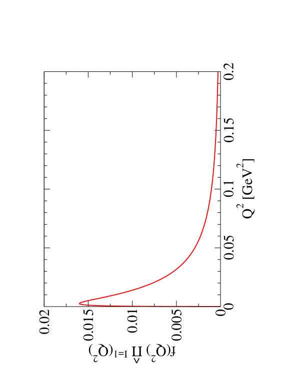
Figure 1: $f(Q^{2})\,\hat{\Pi}^{I=1}(Q^{2})$ versus $Q^{2}$ in the low-$Q^{2}$ region

Figure 1 shows the product of the weight $f(Q^{2})$ appearing in the $a_{\mu}^{\rm LO,HVP}$ integral and the model version of the subtracted $I=1$ polarization. As is well known, this product is strongly peaked at low $Q^{2}$; it is thus shown only in the region $Q^{2}<0.2$ GeV², beyond which it continues to decrease rapidly and monotonically. The model shows the location of the peak to be around $Q^{2}\sim m_{\mu}^{2}/4$. Lattice data typically does not reach such low $Q^{2}$, and some form of fitting is thus necessary to extrapolate into the peak region, at least in the conventional lattice approach.

It is also useful to look at the accumulation of the contributions to $\hat{a}_{\mu}^{\rm LO,HVP}$ as a function of the upper limit of integration, $Q^{2}_{max}$. We display this accumulation, normalized to the integral over all $Q^{2}$, $\hat{a}_{\mu}^{\rm LO,HVP}$, in the model, in Fig. 2. We note that over $80\%$ of the contribution is accumulated below $0.1$ GeV² and over $90\%$ below $0.2$ GeV². It follows that the accuracy required for contributions above $0.1$ or $0.2$ GeV² is much less than that required for the low-$Q^{2}$ region. It thus becomes of interest to investigate the accuracy one might achieve for the higher-$Q^{2}$ contributions were one to avoid altogether fitting and/or modelling, and the associated systematic uncertainty that accompanies it, and instead perform a direct numerical integration over the lattice data. We investigate this question in the next subsection.

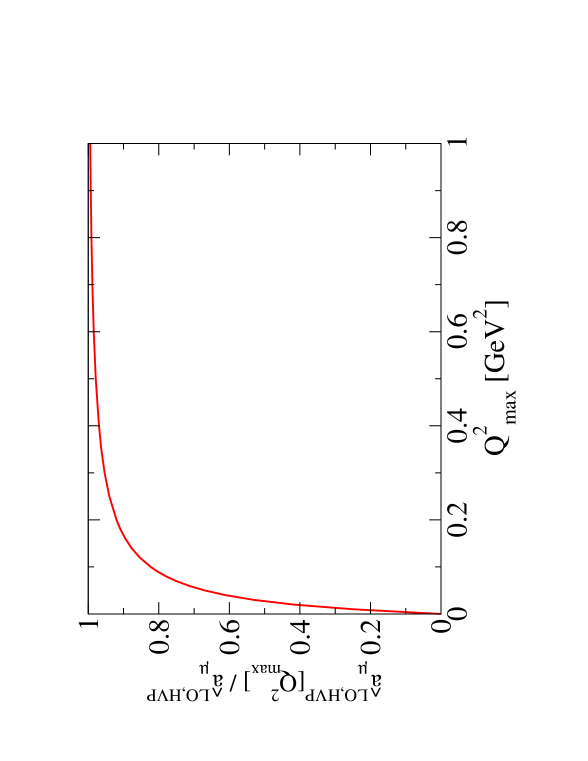
Figure 2: The accumulation of the contributions to $\hat{a}_{\mu}^{\rm LO,HVP}$ as a function of the upper limit, $Q^{2}_{max}$, of integration.

II.3 Direct numerical integration: how low can you go?

In this section, we argue that existing lattice data, even those without twisted boundary conditions, are already sufficiently accurate that direct numerical integration of the lattice data can be relied on to produce a value $\hat{a}_{\mu}^{\rm LO,HVP}[Q^{2}_{min},2$ GeV${}^{2}]$ accurate to well below $1\%$ of $\hat{a}_{\mu}^{\rm LO,HVP}$ for $Q^{2}_{min}$ down to about $0.1$ GeV². The situation will be even better once the results of new data with reduced errors on $\Pi(Q^{2})$ due to all-mode averaging (AMA) bis12 ; amaref and/or denser sets of $Q^{2}$ produced by using twisted boundary conditions DJJW12 ; ABGP13 ; HHJWDJ13 become available.

One practical issue, concerning the constant $\Pi^{I=1}(0)$ needed to convert the unsubtracted polarization $\Pi^{I=1}(Q^{2})$ obtained from the lattice to the corresponding subtracted version $\hat{\Pi}^{I=1}(Q^{2})$ needed for the $I=1$ analogue of the integral in Eq. (1), should be dealt with before continuing with the main investigation of this section. The issue arises because the model we are working with is one for the subtracted polarization. It thus appears to differ from the lattice case, where a determination of $\Pi^{I=1}(0)$ and subsequent subtraction would be required. This issue is, however, easily resolved. One simply interprets the model, not as one for the subtracted polarization, $\hat{\Pi}^{I=1}(Q^{2})$, but rather as one for the unsubtracted polarization, $\Pi^{I=1}(Q^{2})$, happening to have $\Pi^{I=1}(0)=0$ and allows $\Pi^{I=1}(0)$ to become a free parameter in fits of data sets based on our model. left free. The extent to which the fitted $\Pi^{I=1}(0)$ deviates from the known value $0$ then quantifies the systematic uncertainty in the determination of $\Pi^{I=1}(0)$ for the given fit function form.

Fits of $[1,1]$ and higher-order Padé’s on the interval between $0$ and $1$ GeV² to the fake data set of Ref. gmp13 show that it is possible to obtain $\Pi^{I=1}(0)$ from such fits with an uncertainty smaller than $0.001$.

An uncertainty $\delta\Pi^{I=1}(0)$ produces a corresponding uncertainty

$$\delta\hat{a}_{\mu}^{\rm LO,HVP}[Q^{2}_{min}]\,=\,4\alpha^{2}\,\delta\Pi^{I=1}(0)\,\int_{Q^{2}_{min}}^{\infty}dQ^{2}\,f(Q^{2})$$ (5)

on the contribution to $\hat{a}_{\mu}^{\rm LO,HVP}$ from $Q^{2}\geq Q^{2}_{min}$. The rapid decrease of $f(Q^{2})$ with $Q^{2}$ means this uncertainty falls rapidly with increasing $Q^{2}_{min}$. Figure 3 illustrates the impact of this uncertainty on $\hat{a}^{\rm LO,HVP}$. The figure shows the $Q^{2}_{min}$ dependence of $\delta\hat{a}^{\rm LO,HVP}[Q^{2}_{min},\infty]$, as a fraction of $\hat{a}^{\rm LO,HVP}$, for $\delta\Pi^{I=1}(0)=0.001$. Even with this (what we expect to be rather conservative) choice for $\delta\Pi^{I=1}(0)$, the error remains safely below $1\%$ for $Q^{2}_{min}$ down to $0.1$ GeV², where

$$\frac{\delta\hat{a}_{\mu}^{\rm LO,HVP}[0.1\ \mbox{GeV}^{2}]}{\hat{a}_{\mu}^{\rm LO,HVP}}\,=\,0.0074\,\left({\frac{\delta\Pi^{I=1}(0)}{0.001}}\right)\ .$$ (6)

The relatively rapid growth at lower $Q^{2}_{min}$, however, means that careful monitoring of this error for the $\delta\Pi^{I=1}(0)$ actually achieved in a given analysis would be required if one wished to push the lower limit of direct numerical integration of the lattice data to below $0.1$ GeV².

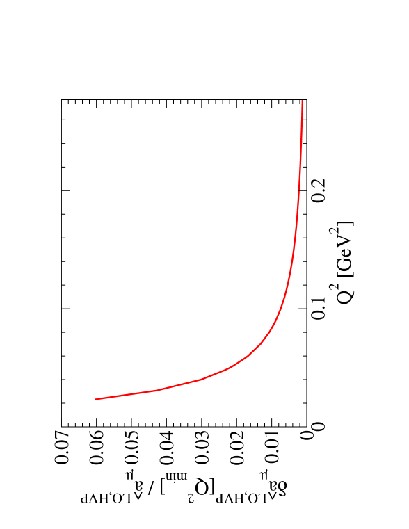
Figure 3: The impact of an uncertainty $\delta\Pi^{I=1}(0)=0.001$ in $\Pi^{I=1}(0)$ on $\hat{a}_{\mu}^{\rm LO,HVP}[Q^{2}_{min},\infty]$ as a fraction of $\hat{a}_{\mu}^{\rm LO,HVP}$.

We now turn to the model study of the accuracy of the direct numerical integration of the subtracted polarization data, assuming that $\delta\Pi^{I=1}(0)$ is small enough to allow for a sufficiently precise subtraction. For this purpose, we employ the fake $I=1$ data set used previously in Ref. gmp13 . The set was constructed from the $\tau$-data-based model discussed above using the covariance matrix for a $64^{3}\times 144$ MILC ensemble with periodic boundary conditions, $a\approx 0.06$ fm and $m_{\pi}\approx 220$ MeV MILC .

The lattice covariance matrix is, by construction, also the covariance matrix of the fake data set. With the fake data and its covariances in hand, we evaluate $\hat{a}_{\mu}^{\rm LO,HVP}[Q^{2}_{min},2$ GeV${}^{2}]$ and its error by direct trapezoid rule integration of the data, and compare the result to the corresponding exact result in the model. The difference between the two gives the systematic error associated with estimating $\hat{a}_{\mu}^{\rm LO,HVP}[Q^{2}_{min},2$ GeV${}^{2}]$ by direct numerical integration.

In addition to this systematic uncertainty, there is, of course, also the statistical component of the overall uncertainty, obtained by propagating the data covariances through the trapezoid-rule evaluation. In the present model study, these covariances are those of the fake data set.

The results for both the systematic and statistical components of the uncertainty on the trapezoid rule evaluation are displayed, as a function of $Q^{2}_{min}$, in Fig. 4. For each $Q^{2}_{min}$, the displayed central value represents the corresponding systematic uncertainty, while the error bar gives the size of the corresponding statistical uncertainty. The results have been scaled by $\hat{a}_{\mu}^{\rm LO,HVP}$ in order to display the impact of the numerical integration uncertainty on the final error for $\hat{a}_{\mu}^{\rm LO,HVP}$. We see that both components are completely negligible above $Q^{2}_{min}\approx 0.2$ GeV². The systematic component remains below $0.25\%$ for all points shown. The statistical component is seen to be dominant for low $Q^{2}_{min}$, reaching about $0.5\%$ for the lowest value shown ($Q^{2}_{min}=0.086$ GeV²). The growth of the statistical component with decreasing $Q^{2}_{min}$ is a consequence of the rapid growth in the data errors for the very low-$Q^{2}$ points, something that would be significantly reduced with improved data bis12 ; amaref .

Figure 4: The systematic and statistical components of the error on the evaluation of $\hat{a}_{\mu}^{\rm LO,HVP}[Q^{2}_{min},2$ GeV${}^{2}]$ by direct trapezoid-rule numerical integration, as a fraction of $\hat{a}_{\mu}^{\rm LO,HVP}$.

The results of this study show that data from existing lattice simulations, even without twisted boundary conditions and/or AMA improvement, allow an evaluation of the contributions to $\hat{a}^{\rm LO,HVP}$ from $Q^{2}>Q^{2}_{min}$ with an accuracy safely below $1\%$ of $\hat{a}^{\rm LO,HVP}$ for $Q^{2}_{min}$ down to at least $0.1$ GeV². While not yet available, analogous fake data sets constructed from covariance matrices corresponding to lattice data with twisted boundary conditions and AMA improvement, will, once available, allow us to quantify the level of improvement made possibly by better statistics and a finer distribution of $Q^{2}$ points. Of course, as explained at the beginning of this subsection, $\Pi^{I=1}(0)$, needed to compute $\hat{\Pi}^{I=1}(Q^{2})$ for the numerical integration, will have to be determined with sufficient precision as well.

The fact that $\hat{a}_{\mu}^{\rm LO,HVP}[Q^{2}_{min},2$ GeV${}^{2}]$ can be reliably evaluated by direct numerical integration down to $Q^{2}_{min}\sim 0.1$ GeV² greatly simplifies the task of computing the rest of the contribution to $\hat{a}_{\mu}^{\rm LO,HVP}$. The reason is that, for $0\leq Q^{2}\,\raisebox{-1.72218pt}{\hbox to0.0pt{$\sim$\hss}}\raisebox{1.72218pt}{$<$}\,0.1$ GeV², one expects fits using low-order Padé’s of the types proposed in Refs. abgp12 ; hpqcd14 , or using the conformal polynomial or chiral representations discussed below (Secs. III.2 and III.3), to provide efficient and reliable representations of the subtracted polarization function. We show that this is indeed the case in the next section, and investigate the systematic uncertainties on the low-$Q^{2}$ contributions produced by the use of such fit forms.

III Behavior of the subtracted polarization in the low-$Q^{2}$ region and a hybrid strategy for evaluating $a_{\mu}^{\rm LO,HVP}$

In the previous section we showed that contributions to $\hat{a}_{\mu}^{\rm LO,HVP}$ from $Q^{2}$ above $\sim 0.1$ GeV² can be obtained with an accuracy better than $1\%$ of $\hat{a}_{\mu}^{\rm LO,HVP}$ by direct numerical integration of existing lattice data. In this section, we discuss the region between $0$ and $\sim 0.1$ GeV² and investigate the reliability of low-order Padé, conformally mapped polynomial, and ChPT representations of the subtracted polarization in this region. We focus on the systematic accuracy achievable using these representations for the evaluation of the low-$Q^{2}$ contributions to $\hat{a}_{\mu}^{\rm LO,HVP}$. As in the previous sections, these investigations are performed using the $\tau$-data-based model for $\hat{\Pi}^{I=1}(Q^{2})$.

At low $Q^{2}$, fits of lattice data to a functional form are needed to achieve a precise determination of the integral in Eq. (1). To avoid difficult-to-quantify systematic errors, the form(s) employed should be free of model dependence. Here we investigate three such functional forms, one based on a sequence of Padé approximants abgp12 ; hpqcd14 , one based on a conformally mapped polynomial, and one based on ChPT. An important question is to what order Padé, what degree conformally mapped polynomial, and what order in the chiral counting one must go in order to obtain representations of $\hat{\Pi}^{I=1}(Q^{2})$ of sufficient accuracy. In addition, there is the question of with what statistical precision these functional forms can then be fit to lattice data. Even if in principle a certain functional form provides an accurate representation of $\hat{\Pi}^{I=1}(Q^{2})$, the parameters still have to be determined with sufficient precision. In this article, we address only the first question, leaving an investigation of the second question to the future, when much more precise lattice data at low $Q^{2}$ are expected to become available.

In order to probe the accuracy of an approximate functional form in representing the exact function $\hat{\Pi}^{I=1}(Q^{2})$, we need to fix the parameters of that form. We will do so by constructing the Padé, conformal and chiral representations such that they reproduce the values of the the relevant low-order derivatives of $\hat{\Pi}^{I=1}(Q^{2})$ with respect to $Q^{2}$ at $Q^{2}=0$. In the model case, these derivatives are known from the dispersive representation of the subtracted polarization, while on the lattice they can be obtained from time moments of the vector current two-point function, as explained in more detail below. Since we are concerned with the systematic uncertainty associated with the use of a given functional form in the low-$Q^{2}$ region, we will assume these derivatives to be exactly known and given by the central values resulting from the dispersive representation. It will still be necessary to reduce the errors on the low-$Q^{2}$ lattice data in order to bring the corresponding statistical uncertainties under control. Our goal is thus only to identify those functional forms which produce systematic uncertainties at the sub-percent level when used with future improved low-$Q^{2}$ data.

III.1 Low-order Padé representations of the subtracted polarization

As already pointed out in Ref. abgp12 , the function $\Phi(Q^{2})\equiv-\hat{\Pi}^{I=1}(Q^{2})/Q^{2}$ is a so-called Stieltjes function and, as such, satisfies a number of theorems on convergent representations over compact regions of the complex $Q^{2}$ plane via Padé approximants multiptpades ; oneptpades . For example, the sequence of $[M+J,M]$ Padé’s constructed to match the first $N=2M+J+1$ coefficients of the Taylor expansion of $\Phi(Q^{2})$ about $Q^{2}=0$ is known to converge to $\Phi(Q^{2})$ as $M\rightarrow\infty$, and for any $J\geq-1$, in any compact set in the complex $Q^{2}$-plane not overlapping the cut of $\hat{\Pi}^{I=1}$ oneptpades . Moreover, for $Q^{2}>0$, the set of such Padé’s satisfies the inequalities oneptpades

$$[0,1]\leq[1,2]\leq\cdots\leq[N,N+1]\leq\Phi(Q^{2})\leq[N,N]\leq\cdots\leq[1,1]\leq[0,0]\ .$$ (7)

To make contact with the notation employed in Ref. hpqcd14 , let us denote $-Q^{2}$ times the $[M,N]$ Padé in (7) by $[M+1,N]_{H}$. The inequalities (7) then correspond to the following inequalities for the Padé representations of $\hat{\Pi}^{I=1}(Q^{2})$

$$[1,0]_{H}\leq[2,1]_{H}\leq\cdots\leq[N+1,N]_{H}\leq\hat{\Pi}^{I=1}(Q^{2})$$

$$\qquad\qquad\leq[N,N]_{H}\leq\cdots\leq[2,2]_{H}\leq[1,1]_{H}\ .$$ (8)

In Ref. hpqcd14 it has been pointed out that the derivatives of the polarization function at $Q^{2}=0$, needed to construct the sequences of Padé’s in Eq. (8), can be determined by evaluating even-order Euclidean time moments of the zero-spatial-momentum representation of the relevant vector current two-point function on the lattice. This idea was implemented for the $\bar{s}s$ and $\bar{c}c$ vector current polarization functions and the resulting representations used to determine the strange and charm contributions to $a_{\mu}^{\rm LO,HVP}$. Evidence was presented that convergence has been achieved by the time the $[2,2]_{H}$ order is reached. However, in the light-quark sector the errors on these moments are expected to be much larger, and to grow rapidly with increasing order, because light-quark correlators are very noisy at large Euclidean $t$. It is, first of all, not clear what order Padé would be required for suitable convergence in the light-quark sector and, second, not obvious that the moments needed to construct, e.g., the $[2,2]_{H}$ Padé can be determined with sufficient accuracy to make the computation of the full light-quark contribution to $a_{\mu}^{\rm LO,HVP}$ feasible in this approach.

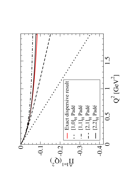
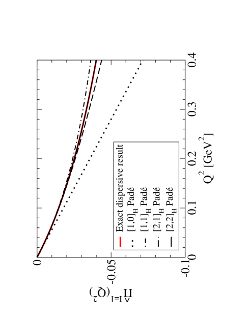
Figure 5: Comparison of the exact dispersive model results for $\hat{\Pi}^{I=1}(Q^{2})$ with the Padé’s constructed from the derivatives of the model with respect to $Q^{2}$ at $Q^{2}=0$ in the intervals $0\leq Q^{2}\leq 2$ GeV² (upper panel) and $0\leq Q^{2}\leq 0.4$ GeV² (lower panel).

The $\tau$-data-based model for $\hat{\Pi}^{I=1}(Q^{2})$ provides a convenient tool for investigating the first of these questions. First, since the exact values of the derivatives of $\hat{\Pi}^{I=1}(Q^{2})$ with respect to $Q^{2}$ at $Q^{2}=0$ in the model are easily obtained from the dispersive representation, Eq. (4), it is straightforward to construct the exact-model versions of the Padé’s of Ref. hpqcd14 and see how well they do in representing $\hat{\Pi}^{I=1}(Q^{2})$. Second, knowing that contributions to $\hat{a}^{\rm LO,HVP}$ from $Q^{2}$ above $\sim 0.1$ GeV² can be accurately determined by direct numerical integration of existing lattice data, we can use the model to explore the obvious question raised by this observation, namely how low an order of Padé will suffice if one’s goal is to evaluate the contribution to $\hat{a}_{\mu}^{\rm LO,HVP}$, not for all $Q^{2}$, but rather only for the restricted region $0\leq Q^{2}\,\raisebox{-1.72218pt}{\hbox to0.0pt{$\sim$\hss}}\raisebox{1.72218pt}{$<$}\,0.1$ GeV².

Figure 5 shows the comparison of the dispersive results for $\hat{\Pi}^{I=1}(Q^{2})$ and the $[1,0]_{H}$, $[1,1]_{H}$, $[2,1]_{H}$, and $[2,2]_{H}$ Padé’s constructed using the exact dispersive results for the derivatives of $\hat{\Pi}^{I=1}(Q^{2})$ with respect to $Q^{2}$ at $Q^{2}=0$. The top panel shows the comparison in the inteval $0\leq Q^{2}\leq 2$ GeV², the bottom panel the same comparison in the more restricted region $0\leq Q^{2}\leq 0.4$ GeV². Note that the curves shown in this figure follow the pattern of the inequalities in Eq. (8). We see that the $[2,2]_{H}$ Padé provides a good, though not perfect, representation of $\hat{\Pi}^{I=1}(Q^{2})$ over the whole of the range $0\leq Q^{2}\leq 2$ GeV². This is not true of the lower-order Padé’s. When one focuses on the low-$Q^{2}$ region, however, it is evident that even the $[1,1]_{H}$ Padé provides a very accurate representation in the region of current interest, $0\leq Q^{2}\leq 0.2$ GeV².

For the problem at hand, of course, it is deviations of the Padé representations from $\hat{\Pi}^{I=1}(Q^{2})$ in the low-$Q^{2}$ region that are of importance in determining the accuracy of the Padé-based estimates for $\hat{a}_{\mu}^{\rm LO,HVP}$. The impact of the deviations seen in Fig. 5 on the contribution $\hat{a}_{\mu}^{\rm LO,HVP}[Q^{2}_{max}]$ from the region $0\leq Q^{2}\leq Q^{2}_{max}$ is shown in Fig. 6 as a function of $Q^{2}_{max}$. The upper panel shows the difference between the various order Padé estimates and the exact model result, scaled as usual by $\hat{a}_{\mu}^{\rm LO,HVP}$, for $Q^{2}_{max}$ in the interval $0\leq Q^{2}_{max}\leq 2$ GeV², while the lower panel zooms in on the region below $0.2$ GeV² of interest here.

We see that, if one insists on using the time moments to evaluate the contributions to $\hat{a}_{\mu}^{\rm LO,HVP}$ from $Q^{2}$ out to $Q^{2}_{max}=2$ GeV² or above, reducing the systematic error on the evaluation to below $1\%$ will require going to the $[2,2]_{H}$ Padé. This would necessitate evaluating time moments with good accuracy out to tenth order, which is likely to be a challenging task for light-quark two-point functions.

We have seen, however, that there is no need to push the moment-based evaluation of $\hat{a}^{\rm LO,HVP}_{\mu}[Q^{2}_{max}]$ out to $Q^{2}_{max}\sim 2$ GeV². In the region below $Q^{2}\sim 0.1-0.2$ GeV² which cannot be handled by direct numerical integration of the lattice data, one does not need the $[2,2]_{H}$ Padé to achieve an accurate representation of $\hat{\Pi}^{I=1}(Q^{2})$. The lower panel of Fig. 6 shows that even the $[1,1]_{H}$ representation is sufficient in this region, producing an estimate for $\hat{a}_{\mu}^{\rm LO,HVP}[Q^{2}_{max}]$ accurate to about 0.3% for $Q^{2}_{max}=0.1$ GeV² and to about $0.5\%$ even for $Q^{2}_{max}=0.2$ GeV². This is a potentially significant advantage since constructing the $[1,1]_{H}$ Padé requires moments only up to sixth order. The $[2,1]_{H}$ Padé lowers the previous errors to $0.06\%$ and $0.2\%$, respectively, but it requires the eighth order moment in its construction.

It is worth emphasizing that another sequence of Padé approximants to $\Pi^{I=1}(Q^{2})$ exists; these are the multi-point Padé’s of Ref. abgp12 , for which convergence theorems also exist multiptpades . These multi-point Padé’s actually have the same form as the single-point, $Q^{2}=0$ Padé’s discussed in Ref. hpqcd14 . Fitting the coefficients of such Padé’s over a relatively low-$Q^{2}$ interval in which the Padé in question is known to provide an accurate representation of $\hat{\Pi}^{I=1}(Q^{2})$ is thus an alternative to obtaining these coefficients by evaluating the time moments of the two-point function. Which of the two approaches will yield the smallest statistical error is a topic for future investigation.

One should, however, bear in mind in this regard that the time moments, in producing the derivatives of the subtracted polarization with respect to $Q^{2}$ at $Q^{2}=0$, will yield Padé’s which, by construction, will be most accurate in the low-$Q^{2}$ region of primary interest for evaluating $\hat{a}_{\mu}^{\rm LO,HVP}$. The deviations of the Padé constructed in this manner from the underlying subtracted polarization will thus lie at higher $Q^{2}$ and have a reduced impact on the error on $\hat{a}_{\mu}^{\rm LO,HVP}$, if the Padé is only used to get the low-$Q^{2}$ contribution. In contrast, in fitting the coefficients of the Padé’s using low-$Q^{2}$ data, the fits will inevitably be more heavily constrained by the somewhat larger $Q^{2}$ points in the fit interval, as these will have smaller errors than the points at very low $Q^{2}$. The resulting Padé may thus be less accurate at very low $Q^{2}$, and one may need to go to a higher-order Padé in comparison to the moment-based approach. Further quantitative investigations of the lattice situation will become possible once covariance matrices corresponding to lattice data with twisted boundary conditions and AMA improvement become available.

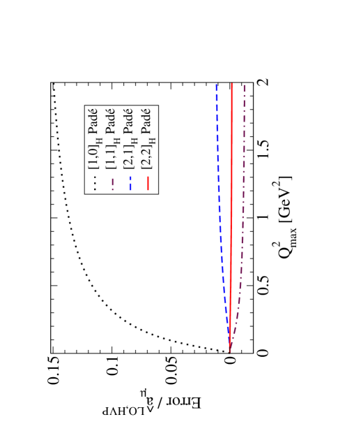
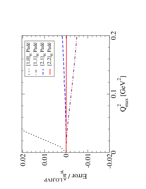
Figure 6: Deviations of the Padé estimates for $\hat{a}_{\mu}^{\rm LO,HVP}[Q^{2}_{max}]$ as a fraction of $\hat{a}_{\mu}^{\rm LO,HVP}$ in the intervals $0\leq Q^{2}_{max}\leq 2$ GeV² (upper panel) and $0\leq Q^{2}_{max}\leq 0.2$ GeV² (lower panel). Note the difference in scale on the vertical axis.

For now, however, we can investigate this issue only using the $I=1$ model data and associated covariance matrix, the latter being generated by the covariances of the experimental $\tau$-decay data used in constructing the model. We emphasize that this covariance matrix is very different from what we may expect any covariance matrix coming from lattice data to look like, so the following short exercise can serve only to address systematic issues, and has nothing to say about the statistics that will be required on the lattice.

If we fit the $\tau$-based data on the interval between $0.1$ and $0.2$ GeV², where lattice errors will typically be much smaller than those at lower $Q^{2}$, we find that it is necessary to go to the $[2,1]_{H}$ Padé if one wishes to reduce the systematic uncertainty on the low-$Q^{2}$ Padé determination of $\hat{a}_{\mu}^{\rm LO,HVP}[0.1$ GeV${}^{2}]$ to the sub-percent level. As an example, a fit to model data at the points $Q^{2}=0.10,\,0.11,\,\cdots,\,0.20$ GeV² using the $[2,1]_{H}$ Padé form, with $\hat{\Pi}^{I=1}(0)$ a free parameter, yields an estimate for $\hat{a}_{\mu}^{\rm LO,HVP}[0.1$ GeV${}^{2}]$ accurate to better than $0.3\%$ of $\hat{a}_{\mu}^{\rm LO,HVP}$. Even more useful, though not unexpected in view of the fact that the $[2,1]_{H}$ representation is essentially indistinguishable from the underlying model polarization out to $Q^{2}\approx 0.2$ GeV², $\hat{a}_{\mu}^{\rm LO,HVP}[Q^{2}_{max}]$ remains accurate to better than $0.3\%$ out to $Q^{2}_{max}=0.2$ GeV². This means that, with sufficiently good data in the interval between $Q^{2}\approx 0.1$ and $0.2$ GeV², one would be able to vary the choice of boundary $Q_{min}^{2}$ between the low-$Q^{2}$ and high-$Q^{2}$ regions and obtain combined hybrid determinations of the full contribution to $a_{\mu}^{\rm LO,HVP}$ for several choices of $Q_{min}^{2}$, providing further checks on the systematics of the hybrid approach.

III.2 Conformal expansion of the subtracted polarization

The Taylor expansion of $\Pi^{I=1}(Q^{2})$ in the variable $Q^{2}$ converges for $|Q^{2}|<4m_{\pi}^{2}$. However, with $4m_{\pi}^{2}=0.078$ GeV², the radius of convergence is most likely too small to be useful in practice. We can improve the convergence properties by rewriting $\Pi^{I=1}(Q^{2})$ first in terms of the variable

$$w(Q^{2})=\frac{1-\sqrt{1+z}}{1+\sqrt{1+z}}\ ,\qquad z=\frac{Q^{2}}{4m_{\pi}^{2}}\ ,$$ (9)

and then expanding in $w$. The series

$$\Pi^{I=1}(Q^{2})=\sum_{n=0}^{\infty}p_{n}w^{n}$$ (10)

should have better convergence properties than the Taylor expansion in $z$, because the whole complex $z$ plane is mapped onto the unit disc in the complex $w$ plane, with the cut $z\in(-\infty,-1]$ mapped onto the disc boundary. The expansion (10) thus has radius of convergence $|w|=1$. In terms of the variable $Q^{2}$, this includes the positive real axis.

For the coefficients $p_{1},\,p_{2},\,\cdots,\,p_{4}$ needed to construct $p(w)$ up to degree $4$, we find, from the derivatives of $\Pi^{I=1}(Q^{2})$ with respect to $Q^{2}$ at $Q^{2}=0$ in the model, the values $p_{1}=0.05565$ and $p_{2}\,=\,-0.06936$, $p_{3}=0.04781$ and $p_{4}\,=\,-0.01561$. The resulting representations of $\hat{\Pi}^{I=1}(Q^{2})$ linear, quadratic, cubic and quartic in $w$ are compared to the exact model values in Fig. 7. We observe, from Figs. 5 and 7, that the Padé and conformal polynomial representations with the same number of parameters lie close to one another.

Let us look more closely at the values of $\hat{a}_{\mu}^{\rm LO,HVP}[Q^{2}_{max}]$ obtained from the conformal polynomial representations. The quadratic version, for example, yields estimates for $\hat{a}_{\mu}^{\rm LO,HVP}[Q^{2}_{max}]$ $0.6\%$ and $1\%$ below the exact model values for $Q^{2}_{max}=0.1$ and $0.2$ GeV², respectively, while the corresponding errors for the cubic representation are $0.02\%$ and $0.04\%$. These numbers are to be compared to $0.3\%$ and $0.5\%$ for the $[1,1]_{H}$ Padé (which has the same number of parameters as the quadratic polynomial), and $0.06\%$ and $0.2\%$ for the $[2,1]_{H}$ Padé (which has same number of parameters as the cubic polynomial).

While the higher-order conformal representations discussed above provide very accurate results for $\hat{a}_{\mu}^{\rm LO,HVP}[Q^{2}_{max}]$, one should bear in mind that their construction requires as input the values of the derivatives of $\hat{\Pi}(Q^{2})$ with respect to $Q^{2}$ at $Q^{2}=0$. As mentioned before, these can, in principle, be obtained from the time moments of the two-point function. Accurate determinations of the relevant moments will thus be required to make the conformal approach useful in this form. It is, of course, also possible to implement the conformal representation by fitting the coefficients of a truncated version of the expansion in Eq. (10) to data on an interval of $Q^{2}$. An exploration of this possibility can be meaningfully carried out in the low-$Q^{2}$ region at present only on the $\tau$-data-based model and its covariances. As in the analogous Padé study in Sec. III.1, we find that a representation one order higher is required to reach the same accuracy for the fitted version as was reached using the corresponding moment approach. Fitting the coefficients of the cubic form to the model data at the points $Q^{2}=0.10,\,0.11,\,\cdots,\,0.20$ GeV², for example, yields estimates for $\hat{a}_{\mu}^{\rm LO,HVP}[Q^{2}_{max}]$ accurate to between $0.6$ and $0.9\%$ for $Q^{2}_{max}$ in the interval from $0.1$ to $0.2$ GeV². The accuracy of the fitted version in this case, though good, is less so than what was achieved for the analogous $[2,1]_{H}$ Padé fit. The Padé approach may thus be favored if one is forced to fit coefficients using data over a limited range of $Q^{2}$, while the conformal approach will be most useful if high-accuracy determinations of the time moments, and hence the derivatives of the polarization at $Q^{2}=0$, turn out to be achievable.

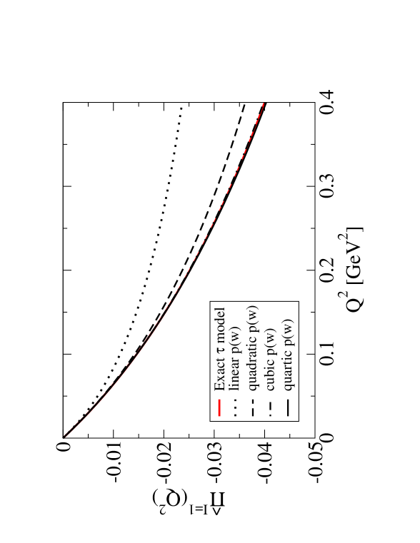
Figure 7: Comparison of the results of the conformal polynomial representations up to quadratic order with the exact $\tau$-data-based model for $\hat{\Pi}^{I=1}(Q^{2})$.

III.3 Chiral representations of the subtracted polarization

In the region of interest, $Q^{2}\,\raisebox{-1.72218pt}{\hbox to0.0pt{$\sim$\hss}}\raisebox{1.72218pt}{$<$}\,0.2$ GeV², $Q^{2}$ is sufficiently small that ChPT should be capable of providing an accurate representation of the subtracted polarization. It has been known for some time that the next-to-leading-order (NLO) representation gl84 ; gl85 ; gk95 ; abt00 is not adequate for this purpose, its slope with respect to $Q^{2}$ being much less than what is seen in either lattice data AB07 or the continuum version of the $I=1$ subtracted polarization discussed above. The source of the problem is the absence, in the NLO representation, of NLO low-energy-constant (LEC) contributions encoding the large contributions associated with the prominent vector meson peaks in the relevant spectral functions. These contributions first appear at NNLO.

The NNLO representation of the subtracted $I=1$ polarization function has the form abt00 ; gk95

$$\left[\hat{\Pi}^{I=1}(Q^{2})\right]_{\rm NNLO}\,=\,{\cal R}(Q^{2};\mu)\,+\,c_{9}(Q^{2};\mu)\,L_{9}^{r}(\mu)\,+\,8\,C_{93}^{r}(\mu)\,Q^{2}\ ,$$ (11)

where $\mu$ is the chiral renormalization scale, $C_{93}^{r}$ is one of the renormalized dimensionful NNLO LECs defined in Refs. bce99 , and ${\cal R}$ and $c_{9}$, which also depend on $m_{\pi}$, $m_{K}$ and $f_{\pi}$, are completely known once $Q^{2}$, $\mu$, $m_{\pi}$, $m_{K}$ and $f_{\pi}$ are specified. The NLO LEC $L_{9}^{r}(\mu)$ is well known from an NNLO analysis of $\pi$ and $K$ electromagnetic form factors bt02 and we take advantage of this determination in the exploratory fits to the $\tau$-based model data below.

In the resonance ChPT (RChPT) approach rchpt , which one expects to represent a reasonable approximation for vector channels, $C_{93}^{r}$ is generated by vector meson contributions. The RChPT result, $C_{93}^{r}\sim-{\frac{f_{V}^{2}}{4m_{V}^{2}}}\simeq\,-0.017$GeV^-2 abt00 , where $f_{V}$ and $m_{V}$ are the vector meson decay constant and mass, is expected to be valid at some typical hadronic scale (usually assumed to be $\mu\sim m_{\rho}$). This rough estimate is well supported by the data, and the term proportional to $C_{93}^{r}$ is, in fact, the dominant contribution to the RHS of Eq. (11) for $Q^{2}\sim 0.1$ GeV².

In the $I=1$ channel, assuming $C_{93}^{r}$ to be dominated by the $\rho$ contribution, and expanding the $\rho$ propagator to one higher order in $Q^{2}$, one obtains an NNNLO contribution of the form $C\,Q^{4}$ which is $-Q^{2}/m_{\rho}^{2}$ times the NNLO contribution $8C_{93}^{r}Q^{2}$, yielding $C\,=\,-8C_{93}^{r}/m_{\rho}^{2}\sim 0.23$ GeV^-4. This estimate leads to a significantly larger curvature of $\hat{\Pi}^{I=1}(Q^{2})$ than predicted by the known lower-order terms and such a larger curvature is indeed clearly indicated by the low-$Q^{2}$ behavior of the $\tau$-data-based model for $\hat{\Pi}^{I=1}(Q^{2})$. Contributions to $\hat{\Pi}^{I=1}(Q^{2})$ from a $C\,Q^{4}$ term with such a value for $C$ already become numerically non-negligible at $Q^{2}\sim 0.1$ GeV². In order to allow accurate chiral fits over the range of interest, we thus need to supplement the NNLO representation of Eq. (11) with an additional $C^{r}Q^{4}$ term. $C^{r}$ represents an effective NNNLO LEC, which is mass-independent at that order. We will refer to the NNLO representation augmented with the $C^{r}Q^{4}$ term as the NN^′LO representation below.

The NN^′LO representation is governed by three LECs, $L_{9}^{r}$, $C^{r}_{93}$ and $C^{r}$, the first of which is already known to better than 10%. The relevant question here is whether, with sufficiently good Euclidean time moments of the vector correlation function, or low-$Q^{2}$ data for its Fourier transform, this form is capable of producing a representation of $\hat{\Pi}^{I=1}(Q^{2})$ accurate enough to allow a sub-percent evaluation of the contribution to $\hat{a}_{\mu}^{LO,HVP}$ from the region $Q^{2}\,\raisebox{-1.72218pt}{\hbox to0.0pt{$\sim$\hss}}\raisebox{1.72218pt}{$<$}\,0.1-0.2$ GeV². It turns out that, at present, the low-$Q^{2}$ errors on data from lattice simulations are still too large, and the $Q^{2}$ coverage too sparse, to allow this question to be sensibly explored using fake data of the type employed in Ref. gmp13 . We thus investigate the systematics of the NN^′LO ChPT fit form using the $\tau$-based $I=1$ model following the same approach as employed in Secs. III.1 and III.2 for the Padé approximant and conformal polynomial forms. In other words, we determine the relevant LECs, and hence the chiral representation, from the values of the derivatives of $\hat{\Pi}^{I=1}(Q^{2})$ with respect to $Q^{2}$ at $Q^{2}=0$ in the model. As mentioned before, in the lattice context these derivatives can, in principle, be determined from the time moments of the Euclidean correlation function.

Using $m_{\pi}=139.57$ MeV, $m_{K}=495.65$ MeV, $f_{\pi}=92.21$ MeV, and $\mu=770$ MeV, as well as $L_{9}^{r}(\mu)=0.00593$ from Ref. bt02 , and the exact values for ${\Pi^{I=1}}^{\prime}(0)$ and ${\Pi^{I=1}}^{\prime\prime}(0)$ from our model, we find that $C_{93}^{r}(\mu)=-0.01567$ GeV^-2 and $C^{r}(\mu)=0.2761$ GeV^-4. Using these values, Fig. 8 shows the comparison between the exact model dispersive results for $\hat{\Pi}^{I=1}(Q^{2})$ and those obtained from the chiral representation (11). Also shown is the chiral representation with the $C^{r}Q^{4}$ contribution removed. The necessity of the NNNLO curvature contribution is evident.

Using our chiral representation, we can compare the value for $\hat{a}_{\mu}^{\rm LO,HVP}[Q^{2}_{max}]$ obtained from NN^′LO ChPT with the exact-model value. For $Q^{2}_{max}=0.1$ GeV², we find that the ChPT value is $0.6\%$ below the exact value, while for $Q^{2}_{max}=0.2$ GeV², it is $1.4\%$ below. While the value at $Q^{2}_{max}=0.1$ GeV² is acceptable, this is clearly worse than the approximation obtained using a $[1,1]_{H}$ Padé determined from the same derivatives at $Q^{2}=0$. NNLO ChPT, which corresponds to setting $C^{r}=0$, yields values of $4\%$ and $18\%$ above the exact value, at $Q^{2}_{max}=0.1$ and $0.2$ GeV², respectively. Clearly, the NN^′LO form provides a good representation for values of $Q^{2}$ extending up to about $0.1$ GeV², but there is evidence for contributions to the curvature in the data at higher $Q^{2}$ beyond that described by the known NLO, NNLO and $C^{r}Q^{4}$ terms. This shows up in the deviations from the data of the chiral curve in the region $Q^{2}\,\raisebox{-1.72218pt}{\hbox to0.0pt{$\sim$\hss}}\raisebox{1.72218pt}{$>$}\,0.1$ GeV² in Fig. 8.

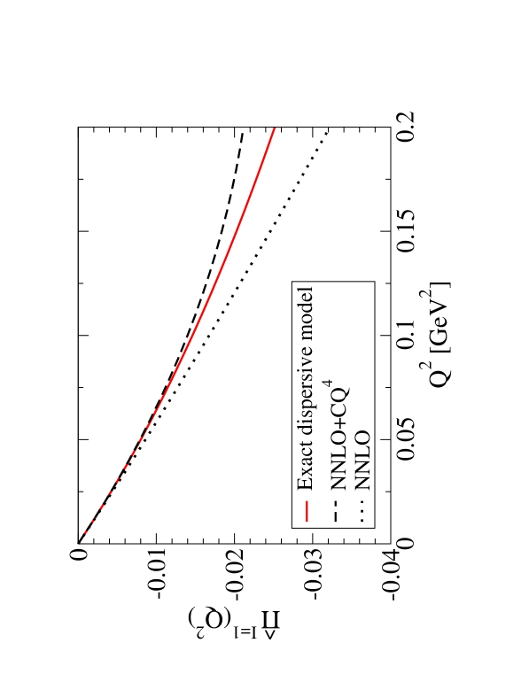
Figure 8: Comparison of the results of the NN^′LO representation (11) and the $\tau$-data-based model for $\hat{\Pi}^{I=1}(Q^{2})$ (solid curve). The dashed line shows the result including the phenomenological term $C^{r}Q^{4}$, the dotted line the result with the NNNLO contribution $C^{r}Q^{4}$ removed.

As in the case of Padé’s, an alternative method for constructing a chiral representation for $\Pi^{I=1}(Q^{2})$ is by fits to lattice data at non-zero values of $Q^{2}$, instead of from derivatives at $Q^{2}=0$. Such fits will be most reliable when employed in a fit window involving as low $Q^{2}$ as possible. From Fig. 8 and the discussion above, it follows that data at values of $Q^{2}$ below 0.1 GeV² would be needed. In the case of fits to Padé’s, we saw in Sec. III.1 that a sufficiently accurate representation can in principle be obtained from data in an interval farther away from zero, $0.1\,\raisebox{-1.72218pt}{\hbox to0.0pt{$\sim$\hss}}\raisebox{1.72218pt}{$<$}\,Q^{2}\,\raisebox{-1.72218pt}{\hbox to0.0pt{$\sim$\hss}}\raisebox{1.72218pt}{$<$}\,0.2$ GeV² if one increases the order of the Padé from $[1,1]_{H}$ to $[2,1]_{H}$ by adding one parameter. In ChPT, such an approach would imply going beyond NNNLO order. (As it is, even the NN^′LO representation is only a phenomenological version of the NNNLO representation.) With such high orders not being available, the application of ChPT is limited to the moment-based approach, or possibly to fits at $Q^{2}$ values below 0.1 GeV². This means the ChPT approach to the low-$Q^{2}$ region, though potentially providing a consistency check, is likely to be less useful than the Padé approach. The former requires small-error data at as low as possible $Q^{2}$ (something more difficult to accomplish in practice) while, as shown in Sec. III.1, a $[2,1]_{H}$ Padé representation obtained by fitting to good quality data restricted to the somewhat higher region of $Q^{2}$ between approximately $0.1$ and $0.2$ GeV² can be employed to obtain a sufficiently accurate value for $\hat{a}_{\mu}^{\rm LO,HVP}[Q^{2}_{max}]$ out to $Q^{2}_{max}=0.2$ GeV². The Padé approach, whether implemented through moments or through fitting, is thus likely to be a more favorable one from a practical point of view.

To summarize the conclusions of this subsection, we have shown that, in the region $0<Q^{2}\,\raisebox{-1.72218pt}{\hbox to0.0pt{$\sim$\hss}}\raisebox{1.72218pt}{$<$}\,0.1$ GeV², use of NN^′LO ChPT provides a representation of the subtracted polarization accurate enough to allow the evaluation of $a_{\mu}^{\rm LO,HVP}[0.1$ GeV${}^{2}]$ with a systematic error at the sub-percent level. Because lattice data at $Q^{2}$ values below 0.1 GeV² will be required to reach this level, however, use of this ChPT-inspired fit form is likely to produce results for $a_{\mu}^{\rm LO,HVP}[0.1$ GeV${}^{2}]$ with larger errors than those obtained from Padé-based approaches.

We conclude this subsection with a brief discussion of the low-$Q^{2}$ $I=0$ contributions to $a_{\mu}^{\rm LO,HVP}$. As discussed above, the NN^′LO fits to the model $\hat{\Pi}^{I=1}(Q^{2})$ data fix the LECs $C_{93}^{r}$ and $C^{r}$. It turns out that at NNLO the related subtracted vector isoscalar polarization function, $\hat{\Pi}^{I=0}(Q^{2})$, is determined by the same set of LECs as is $\hat{\Pi}^{I=1}(Q^{2})$ abt00 . This statement remains true of the NN^′LO form as well. The chiral fit thus also provides us with what should be an accurate expectation for the behavior of $\hat{\Pi}^{I=0}(Q^{2})$ in the low-$Q^{2}$ region. In the isospin limit, $\hat{\Pi}^{I=0}(Q^{2})$ determines the $I=0$ contribution to $a_{\mu}^{\rm LO,HVP}$ via

$$\left[a_{\mu}^{\rm LO,HVP}\right]^{I=0}\,=\,-2\alpha^{2}\,\int_{0}^{\infty}dQ^{2}\,f(Q^{2})\,{\frac{1}{3}}\,{\hat{\Pi}^{I=0}}(Q^{2})\ .$$ (12)

Fig. 9 shows the NN^′LO expectation for the product $f(Q^{2})\hat{\Pi}^{I=0}(Q^{2})$ appearing in the integrand of Eq. (12). The corresponding $I=1$ product $f(Q^{2})\hat{\Pi}^{I=1}(Q^{2})$ is included for comparison. It is clear that, though the $Q^{2}$ dependence of the two is not identical, the behavior of the $I=0$ integrand is sufficiently similar to that of the $I=1$ integrand that our conclusions regarding the low-$Q^{2}$ $I=1$ contribution to $a_{\mu}^{\rm LO,HVP}$ will also hold for the $I=0$ contribution.

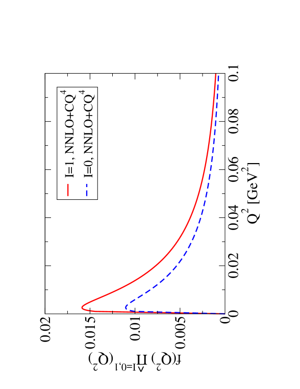
Figure 9: The NN^′LO ChPT expectation for the low-$Q^{2}$ behavior of the integrand for the $I=0$ contribution to $a_{\mu}^{LO,HVP}$. Also shown, for comparison, is the integrand for the corresponding $I=1$ contribution.

IV Errors for the hybrid strategy and conclusions

We have shown that the problem of determining the LO HVP contribution to $a_{\mu}$ on the lattice can be profitably approached through a hybrid strategy in which contributions from $Q^{2}\geq Q_{min}^{2}$ are evaluated by direct trapezoid rule numerical integration of lattice data for the subtracted polarization and those from the low-$Q^{2}$ region, $0\leq Q^{2}\leq Q_{min}^{2}$, by other methods. Existing lattice data produced in simulations using periodic boundary conditions, even without further improvements such as AMA and/or the use of twisted boundary conditions, are already sufficiently precise to allow the $Q^{2}\geq Q_{min}^{2}$ contributions to be obtained with systematic and statistical errors well below $1\%$ of $a_{\mu}^{\rm LO,HVP}$ for $Q_{min}^{2}$ as low as $0.1$ GeV².

In evaluating contributions from the region of $Q^{2}$ below $Q_{min}^{2}\sim 0.1$ GeV², we have shown, by studying a physical model of the $I=1$ vector polarization function, that low-order Padé’s, conformally mapped polynomials, as well as NN^′LO ChPT (NNLO ChPT supplemented by an additional curvature contribution whose physical origin is understood) provide forms capable of representing the subtracted polarization with sufficient accuracy to reduce the systematic uncertainty arising from computing $\hat{a}_{\mu}^{\rm LO,HVP}[Q_{min}^{2}]$ using these forms to a level well below $1\%$ of $\hat{a}_{\mu}^{\rm LO,HVP}$. In the case of the low-order Padé’s, this conclusion remains in force for $Q_{min}^{2}$ out to beyond $0.2$ GeV². In contrast, systematic errors associated with the use of the NN^′LO ChPT form grow to about $1.4\%$ of $\hat{a}_{\mu}^{\rm LO,HVP}$ for $Q_{min}^{2}\sim 0.2$ GeV².

A promising approach to the low-$Q^{2}$ region, from a systematic point of view, appears to be that involving the Padé’s constructed from the derivatives of the polarization function with respect to $Q^{2}$ at $Q^{2}=0$. These derivatives can be obtained from time moments of the zero-spatial-momentum two-point function hpqcd14 . The hybrid approach allows use of a lower order than would otherwise be possible, with the $[1,1]_{H}$ Padé already being sufficient to produce a systematic error on the determination of $\hat{a}_{\mu}^{LO,HVP}[Q_{min}^{2}]$ safely below $1\%$ for $Q_{min}^{2}$ out to beyond $0.2$ GeV². Reducing the order of the Padé employed has the advantage of reducing the order to which the time moments must be evaluated with good accuracy, and thus represents a practical advantage in view of the expectation that light-quark moment errors will grow rapidly with increasing order. Constructing the $[1,1]_{H}$ Padé requires moments only out to sixth order. In contrast, evaluating the contribution to $\hat{a}_{\mu}^{\rm LO,HVP}$ out to $2$ GeV² with sub-percent accuracy, would require at least the $[2,2]_{H}$ Padé, and hence time moments out to at least tenth order.

We have also shown that a multi-point implementation of the Padé approach abgp12 , in which the parameters of the Padé’s are fit rather than obtained from moments, is also feasible. This version has the advantage that, with sufficiently good data, it can be successfully implemented using only data from the region of $Q^{2}$ between approximately $0.1$ and $0.2$ GeV², where lattice data errors are typically significantly smaller than at lower $Q^{2}$. To reach sub-percent accuracy in this implementation, however, requires going to the $[2,1]_{H}$ Padé.

The approach using polynomials in the conformally transformed variable $w$ also looks promising, provided again that moment evaluations of the derivatives of $\Pi(Q^{2})$ with respect to $Q^{2}$ at $Q^{2}=0$ reach a sufficient level of accuracy. If one is forced to estimate the polynomial coefficients by fitting, however, this approach looks less favorable than the corresponding Padé approach.

While in principal also usable, the ChPT-based approach appears to us to require better lattice data to reach the same level of precision than do the two Padé approaches. This is a consequence of (i) the necessity of performing the NN^′LO fits on intervals restricted to $Q^{2}\,\raisebox{-1.72218pt}{\hbox to0.0pt{$\sim$\hss}}\raisebox{1.72218pt}{$<$}\,0.1$ GeV² if one wishes to keep the associated systematic errors at the sub-percent level, and (ii) the fact that errors on lattice data are typically significantly larger below $Q^{2}\sim 0.1$ GeV² than they are in the interval between $0.1$ and $0.2$ GeV².

Current low-$Q^{2}$ lattice data are not yet sufficiently precise to produce sub-percent level statistical errors on the low-$Q^{2}$ contributions $a_{\mu}^{\rm LO,HVP}[Q_{min}^{2}]$. To understand what might be required to reach the desired precision, it is convenient to consider the case of the moment approach, specifically the $[1,1]_{H}$ Padé representation of the subtracted polarization,

$$\hat{\Pi}(Q^{2})\,=\,\Pi(Q^{2})-\Pi(0)\,=\,{\frac{a_{1}Q^{2}}{1+b_{1}Q^{2}}}\,,$$ (13)

which we know is sufficient to produce systematic uncertainties well below $1\%$. Errors $\delta a_{1}$ and $\delta b_{1}$ on the parameters $a_{1}$ and $b_{1}$ produce associated errors

$$\delta_{a_{1}}a_{\mu}^{LO,HVP}[Q_{min}^{2}]\, =\,-4\alpha^{2}\,\int_{0}^{Q_{min}^{2}}dQ^{2}\,f(Q^{2})\,\left({\frac{Q^{2}}{1+b_{1}Q^{2}}}\right)\delta a_{1}\ ,$$

$$\delta_{b_{1}}a_{\mu}^{LO,HVP}[Q_{min}^{2}]\, =\,-4\alpha^{2}\,\int_{0}^{Q_{min}^{2}}dQ^{2}\,f(Q^{2})\,\left({-\frac{a_{1}Q^{4}}{(1+b_{1}Q^{2})^{2}}}\right)\delta b_{1}\ .$$ (14)

on $a_{\mu}^{\rm LO,HVP}[Q_{min}^{2}]$. Let us now consider the $I=1$ analogue, for which we can quantify these uncertainties using our $\tau$-data-based model. Taking the central values for $a_{1}$ and $b_{1}$ from the $[1,1]_{H}$ Padé version obtained from the derivatives of the model polarization with respect to $Q^{2}$ at $Q^{2}=0$, scaling the errors, as usual, by $\hat{a}_{\mu}^{\rm LO,HVP}$, and defining $c_{a_{1}}[a_{1},b_{1},Q^{2}_{min}]$ and $c_{b_{1}}[a_{1},b_{1},Q^{2}_{min}]$ by

$${\frac{\delta_{a_{1}}\hat{a}_{\mu}^{\rm LO,HVP}[Q_{min}^{2}]}{\hat{a}_{\mu}^{\rm LO,HVP}}}\, =\,c_{a_{1}}[a_{1},b_{1},Q^{2}_{min}]\,{\frac{\delta a_{1}}{a_{1}}}$$

$${\frac{\delta_{b_{1}}\hat{a}_{\mu}^{\rm LO,HVP}[Q_{min}^{2}]}{\hat{a}_{\mu}^{\rm LO,HVP}}}\, =\,c_{b_{1}}[a_{1},b_{1},Q^{2}_{min}]\,{\frac{\delta b_{1}}{b_{1}}}\ ,$$ (15)

we find, for example, that

$$c_{a_{1}}[a_{1},b_{1},\,0.1\ \mbox{GeV}^{2}] = 0.818\ ,$$

$$c_{b_{1}}[a_{1},b_{1},\,0.1\ \mbox{GeV}^{2}] = -0.0488\ ,$$ (16)

and

$$c_{a_{1}}[a_{1},b_{1},\,0.2\ \mbox{GeV}^{2}] = 0.913\ ,$$

$$c_{b_{1}}[a_{1},b_{1},\,0.2\ \mbox{GeV}^{2}] = -0.0724\ .$$ (17)

It follows that a sub-percent error on $a_{1}$ will be sufficient to obtain a sub-percent error on $\hat{a}_{\mu}^{\rm LO,HVP}[Q_{min}^{2}]$ for $Q_{min}^{2}\leq 0.2$ GeV², provided the errors on $b_{1}$ remain at the few percent level, regardless of how correlated the fit parameters $a_{1}$ and $b_{1}$ might be. The parameter $a_{1}$ is determined by the slope of the subtracted polarization with respect to $Q^{2}$ at $Q^{2}=0$, and $b_{1}$ by the ratio of the curvature to the slope. A useful rule-of-thumb goal emerging from this exercise is thus that, to reach the sub-percent error level, one should aim at reducing the error on the slope parameter $a_{1}$, whether obtained from the fourth-order time moment, or from fitting, to the sub-percent level. Further quantitative studies using our $\tau$-based model will become possible once covariance matrices associated with AMA-improved data with twisted boundary conditions become available. This will allow us to construct fake data sets based on the model but with realistic errors and correlations from the point of view of the lattice.

- (1) G.W. Bennett et al. [The Muon g-2 Collaboration], Phys. Rev. Lett. 92, 161802 (2004) [hep-ex/0401008]; Phys. Rev. D73, 072003 (2006) [hep-ex/0602035].
- (2) See, for instance, F. Jegerlehner and A. Nyffeler, Phys. Rept. 477, 1 (2009) [arXiv:0902.3360 [hep-ph]]; M. Davier, A. Höcker, B. Malaescu and Z.Q. Zhang, Eur. Phys. J. C 71, 1515 (2011) [Erratum-ibid. C 72, 1874 (2012)] [arXiv:1010.4180 [hep-ph]]; T. Blum, A. Denig, I. Logashenko, E. de Rafael, B. Lee Roberts, T. Teubner and G. Venanzoni, arXiv:1311.2198 [hep-ph], and references therein.
- (3) T. Aoyama, M. Hayakawa, T. Kinoshita and M. Nio, Phys. Rev. Lett. 109, 111808 (2012) [arXiv:1205.5370 [hep-ph]].
- (4) R. R. Akhmetshin et al. [CMD-2 Collaboration], Phys. Lett. B648, 28 (2007) [hep-ex/0610021].
- (5) M. N. Achasov, K. I. Beloborodov, A. V. Berdyugin, A. G. Bogdanchikov, A. V. Bozhenok, A. D. Bukin, D. A. Bukin and T. V. Dimova, et al., J. Exp. Theor. Phys. 103, 380 (2006) [Zh. Eksp. Teor. Fiz. 130, 437 (2006)] [hep-ex/0605013].
- (6) J. P. Lees, et al. [BaBar Collaboration], Phys. Rev. D86, 032013 (2012) [arXiv:1205.2228 [hep-ex]].
- (7) D. Babusci, et al. [KLOE Collaboration], Phys. Lett. B720, 336 (2013) [arXiv:1212.4524 [hep-ex]].
- (8) For a recent review, see T. Blum, M. Hayakawa and T. Izubuchi, PoS LATTICE 2012, 022 (2012) [arXiv:1301.2607 [hep-lat]].
- (9) T. Blum, Phys. Rev. Lett. 91, 052001 (2003) [hep-lat/0212018].
- (10) C. Aubin and T. Blum, Phys. Rev. D75, 114502 (2007) [arXiv:hep-lat/0608011].
- (11) X. Feng, K. Jansen, M. Petschlies and D. B. Renner, Phys. Rev. Lett. 107, 081802 (2011) [arXiv:1103.4818 [hep-lat]]; X. Feng, G. Hotzel, K. Jansen, M. Petschlies and D. B. Renner, PoS LATTICE 2012, 174 (2012) [arXiv:1211.0828 [hep-lat]].
- (12) P. Boyle, L. Del Debbio, E. Kerrane and J. Zanotti, Phys. Rev. D85, 074504 (2012) [arXiv:1107.1497 [hep-lat]].
- (13) M. Della Morte, B. Jäger, A. Jüttner and H. Wittig, JHEP 1203, 055 (2012) [arXiv:1112.2894 [hep-lat]]; PoS LATTICE 2012, 175 (2012) [arXiv:1211.1159 [hep-lat]].
- (14) C. Aubin, T. Blum, M. Golterman and S. Peris, Phys. Rev. D 86, 054509 (2012) [arXiv:1205.3695 [hep-lat]].
- (15) G. M. de Divitiis, R. Petronzio and N. Tantalo, Phys. Lett. B 718, 589 (2012) [arXiv:1208.5914 [hep-lat]].
- (16) X. Feng, S. Hashimoto, G. Hotzel, K. Jansen, M. Petschlies and D. B. Renner, Phys. Rev. D88, 034505 (2013) [arXiv:1305.5878 [hep-lat]].
- (17) A. Francis, B. Jäger, H. B. Meyer and H. Wittig, Phys. Rev. D88, 054502 (2013) [arXiv:1306.2532 [hep-lat]].
- (18) C. Aubin, T. Blum, M. Golterman and S. Peris, Phys. Rev. D88, 074505 (2013) [arXiv:1307.4701 [hep-lat]].
- (19) F. Burger, X. Feng, G. Hotzel, K. Jansen, M. Petschlies and D. B. Renner, JHEP 1402, 099 (2014) [arXiv:1308.4327 [hep-lat]].
- (20) M. Golterman, K. Maltman and S. Peris, Phys. Rev. D88, 114508 (2013) [arXiv:1309.2153 [hep-ph]].
- (21) H. Horch, G. Herdoiza, B. Jäger, H. Wittig, M. Della Morte and A. Jüttner, PoS LATTICE 2013, 304 (2013) [arXiv:1311.6975 [hep-lat]].
- (22) B. Chakraborty, et al., arXiv:1403.1778 [hep-lat].
- (23) B. E. Lautrup, A. Peterman and E. de Rafael, Phys. Rept. 3, 193 (1972).
- (24) T. Blum, T. Izubuchi and E. Shintani, Phys. Rev. D 88, 094503 (2013) [arXiv:1208.4349 [hep-lat], arXiv:1208.4349 [hep-lat]].
- (25) E. Shintani, et al., arXiv:1402.0244 [hep-lat].
- (26) R. Barate, et al. [ALEPH Collaboration], Z. Phys. C76, 15 (1997); R. Barate, et al. [ALEPH Collaboration], Eur. Phys. J C4, 409 (1998); S. Schael et al. [ALEPH Collaboration], Phys. Rep. 421, 191 (2005) [hep-ex/0506072].
- (27) K. Ackerstaff et al. [OPAL Collaboration], Eur. Phys. J. C7, 571 (1999) [hep-ex/9808019].
- (28) D. Boito, et al., Phys. Rev. D85, 093015 (2012) [arXiv:1203.3146 (hep-ph)].
- (29) P. A. Baikov, K. G. Chetyrkin and J. H. Kühn, Phys. Rev. Lett. 101 (2008) 012002 [arXiv:0801.1821 [hep-ph]].
- (30) O. Catà, M. Golterman and S. Peris, JHEP 0508, 076 (2005) [hep-ph/0506004]; Phys. Rev. D77, 093006 (2008) [arXiv:0803.0246 [hep-ph]].
- (31) B. Blok, M. A. Shifman and D. X. Zhang, Phys. Rev. D57, 2691 (1998) [Erratum-ibid. D59, 019901 (1999)] [arXiv:hep-ph/9709333]; I. I. Y. Bigi, M. A. Shifman, N. Uraltsev, A. I. Vainshtein, Phys. Rev. D59, 054011 (1999) [hep-ph/9805241]; M. A. Shifman, [hep-ph/0009131]; M. Golterman, S. Peris, B. Phily, E. de Rafael, JHEP 0201, 024 (2002) [hep-ph/0112042].
- (32) MILC collaboration, http://physics.indiana.edu/sg/milc.html .
- (33) G.A. Baker Jr., J. Math. Phys. 10, 814 (1969); M. Barnsley, J. Math. Phys. 14, 299 (1973).
- (34) G.A. Baker, P. Graves-Morris, “Pade Approximants”, Addison Wesley, 1981.
- (35) J. Gasser and H. Leutwyler, Ann. Phys. 158, 142 (1984).
- (36) J. Gasser and H. Leutwyler, Nucl. Phys. B250, 465 (1985).
- (37) E. Golowich and J. Kambor, Nucl. Phys. B 447, 373 (1995) [hep-ph/9501318].
- (38) G. Amoros, J. Bijnens and P. Talavera, Nucl. Phys. B568, 319 (2000) [hep-ph/9907264].
- (39) J. Bijnens, G. Colangelo and G. Ecker, JHEP 02, 020 (1999) [hep-ph/9902437]; Ann. Phys. 280, 100 (2000) [hep-ph/9907333].
- (40) J. Bijnens and P. Talavera, JHEP 0203, 046 (2002) [hep-ph/0203049].
- (41) G. Ecker, J. Gasser, A. Pich and E. de Rafael, Nucl. Phys. B321 311 (1989).