Unconventional Quantum Criticality due to Critical Valence Transition

Abstract

Quantum criticality due to the valence transition in some Yb-based heavy fermion metals has gradually turned out to play a crucial role to understand the non-Fermi liquid properties that cannot be understood from the conventional quantum criticality theory due to magnetic transitions. Namely, critical exponents giving the temperature ($T$) dependence of the resistivity $\rho(T)$, the Sommerfeld coefficient, $C(T)/T$, the magnetic susceptibility, $\chi(T)$, and the NMR relaxation rates, $1/(T_{1}T)$, can be understood as the effect of the critical valence fluctuations of $f$ electrons in Yb ion in a unified way. There also exist a series of Ce-based heavy fermion metals that exhibit anomalies in physical quantities, enhancements of the residual resistivity $\rho_{0}$ and the superconducting critical temperature ($T_{\rm c}$) around the pressure where the valence of Ce sharply changes. Here we review the present status of these problems both from experimental and theoretical aspects.

1 Introduction

Since the mid 1990’s, the physics of quantum critical phenomena has been intensively discussed in the heavy fermion community. This is reasonable because the heavy fermions usually arise in nearly magnetic materials, in which strong local correlation due to the strong local Coulomb repulsion of the order of 1 Ryd ($\simeq$13.6 eV) works among $f$-electrons at rare earth or actinide ions. For example, CeCu₂Si₂, the first heavy fermion superconductor discovered by Steglich et al. in 1979, [1] has now turned out to be located close to the quantum critical point where the spin density wave state disappears. [2] A series of compounds were reported to exhibit magnetic quantum critical point under pressure around which an unconventional superconductivity appears: e.g., in CePd₂Si₂ [3], CeIn₃ [4], and CeRh₂Si₂ [5]. As for the mechanism of superconductivity, the “antiferromagnetic” spin fluctuation mechanism was proposed in mid 1980’s. [6, 7] After that, its strong coupling treatments have been developed [8] and also for a mechanism of high-$T_{\rm c}$ cuprates and some organic superconductors. [9]

On the other hand, an importance of valence fluctuations was already suggested as an origin for an enhancement of the superconducting (SC) transition temperature $T_{\rm c}$ of CeCu₂Si₂ under pressure by Bellarbi et al. in 1984, [10] at relatively early stage of research in heavy fermion superconductivity. The Kondo-volume-collapse mechanism for CeCu₂Si₂ proposed by Razafimandaby et al. at the same stage is also based on a kind of valence fluctuation idea. [11] In SCES conference at Paris in 1998, Jaccard reported comprehensive data on pressure-induced superconductivity in CeCu₂Ge₂, a sister compound of CeCu₂Si₂, together with anomalous properties in its normal state, [12] in which a close relationship between the enhancement of $T_{\rm c}$ and a sharp valence crossover of Ce ion from Kondo to valence-fluctuation regime was explicitly shown. Theoretical attempts to coherently understand these experimental results have been performed since then. [13, 14, 15, 16, 18, 17] Similar detailed measurements, including specific heat measurement under pressure, in CeCu₂Si₂ was also reported by Holmes et al., [18] on the basis of almost local critical valence fluctuation scenario. A remarkable report on CeCu₂(Si_0.9Ge_0.1)₂ by Yuan et al. [19] also eloquently indicated the existence of the valence fluctuation mechanism other than that due to critical “antiferromagnetic” fluctuations, because the $T_{\rm c}$ exhibits two domes, one at the magnetic quantum critical pressure and another at the pressure where the valence of Ce ion changes sharply as in the case of CeCu₂Si₂ and CeCu₂Ge₂.

These findings show that only the so-called Doniach phase diagram, [20] a sort of dogma in heavy fermion physics, is not sufficient to fully understand the physics of heavy fermions. In other words, the Kondo lattice model, in which the $f$ electron number $n_{\rm f}$ per ion is fixed as $n_{\rm f}=1$, would not be a sufficient model but the Anderson lattice model offers us a better starting point. A prototypical valence transition phenomenon is a $\gamma$-$\alpha$ transition of Ce metal that exhibits the first order valence transition at $P\simeq 1.0$ GPa from Ce^+3.03 to Ce^+3.14 at $T=300$K and has a critical end point (CEP) at $T\simeq 600$K and $P\simeq 2.0$GPa. [21] There were roughly two ways to understand the valence transition in rare earth ions: Kondo volume collapse (KVC) model and extended periodic Anderson model (PAM) or extended Falicov-Kimball model (FKM).

The KVC model uses the fact that the Kondo temperature $T_{\rm K}$, representing the energy gain due to the Kondo effect or correlation, has a sharp pressure (volume) dependence through the c-f exchange interaction. Then, the valence transition is discussed in terms of the Gibbs free energy. [22, 23, 24] Although it describes quite well a $P$-$V$ or $P$-$T$ phase diagram of the $\gamma$-$\alpha$ transition of Ce metal and other Ce- or Yb-based heavy fermions, the criticality is not directly related with the valence change nor to the response of electron degrees of freedom but with volume or strain of the crystal. Therefore, the relation between microscopic model and phenomena is not straightforward as far as we understand. For example, it seems not so simple to understand possible magnetic anomalies near the quantum critical end point (QCEP) of valence transition, such as anomalous temperature ($T$) dependences in magnetic susceptibility and NMR/NQR relaxation rates. (See §3.)

On the other hand, the FKM directly discusses the valence state of rare earth ions by considering the condition how it is influenced by the effect of the Coulomb repulsion $U_{\rm fc}$ between $f$- and conduction electrons. [25, 26] However, original FKM includes no c-f hybridization which is the heart of the valence fluctuation problem including the Kondo effect. After that, theoretical efforts have been performed to take into account the hybridization effect in a form or another in the case of lattice systems [27, 28] or as the impurity problem. [29, 30, 31, 32] The Hamiltonian of the extended PAM or extended FKM is given as

$$H_{\rm EPAM} = \sum_{{\bf k}\sigma}(\epsilon_{\bf k}-\mu)c_{{\bf k}\sigma}^{\dagger}c_{{\bf k}\sigma}+\varepsilon_{\rm f}\sum_{{\bf k}\sigma}f_{{\bf k}\sigma}^{\dagger}f_{{\bf k}\sigma}+U_{\rm ff}\sum_{i}n_{i\uparrow}^{\rm f}n_{i\downarrow}^{\rm f}$$ (1)

$$\qquad+V\sum_{{\bf k}\sigma}(c_{{\bf k}\sigma}^{\dagger}f_{{\bf k}\sigma}+{\rm h.c.})+U_{\rm fc}\sum_{i\sigma\sigma^{\prime}}n_{i\sigma}^{\rm f}n_{i\sigma^{\prime}}^{\rm c},$$

where $U_{\rm fc}$, the f-c Coulomb repulsion, is included other than the conventional PAM. Here, it should be noted that $\sigma$ in eq. (1) stands for the label specifying the degrees of freedoms of the Kramers doublet state of the ground crystalline-electric-field (CEF) level. If there is no hybridization, $V=0$, the condition of valence transition is given by

$$\varepsilon_{\rm f}+n_{\rm c}U_{\rm fc}=\mu,$$ (2)

where $\mu$ is the chemical potential or the Fermi level in the Kondo limit where $f$ electrons are essentially singly occupied. Even in the case $V\not=0$, this condition is valid in the mean-field level of approximation. Figure 1 shows the ground state phase diagrams in the $\varepsilon_{\rm f}$-$U_{\rm fc}$ plane that is obtained by the mean-field approximation using the slave boson technique by taking into account the strong correlation effect ($U_{\rm ff}=\infty$), and by the density-matrix-renormalization-group (DMRG) method for the one-dimensional version of the Hamiltonian eq. (1). [17] Calculations on the Gutzwiller variational ansatz have also been performed. [15, 33, 34, 35, 36] The first order valence transition line is given essentially by condition (2). The QCEP (closed circles) for the first order valence transition (line) shifts from the position given by the mean-field approximation to that given by asymptotically exact DMRG calculation due to the strong quantum fluctuation effect. In this approach based on the extended FKM or extended PAM, properties of electronic state associated with the valence change or critical fluctuations can be directly calculated within a required accuracy as shown in §3.

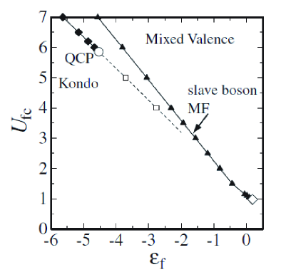
Figure 1: Phase diagram at $T=0$ of the system described by the Hamiltonian (1) in $\varepsilon_{\rm f}-U_{\rm fc}$ plane. Triangles (diamonds and squares) are the results by the slave-boson mean-field approximation (DMRG calculations for the one dimensional (1d) version of the Hamiltonian (1) ). Solid lines represent the first order valence transition, and dashed line represent that for the valence crossover from Kondo to mixed valence regime. Closed circles are critical end point of the first order valence transition, i.e., quantum crtical point of valence transition. Parameters are $V/t=0.1$, $U_{\rm ff}/t=100$, $t$ being the transfer integral of tight-binding model for the conduction band in the 1d version of the Hamiltonian (1), and the total electron number per unit cell, $n$, is fixed as $n=7/8$, the same as used in ref. Onishi1. Unit of $U_{\rm fc}$ and $\varepsilon_{\rm f}$ are also $t$.

Another important issue is how to understand the unconventional quantum critical phenomena observed in a series of materials, [37, 38, 39, 40, 41, 42, 43, 44] in which the critical exponent of $T$ dependence in various physical quantities cannot be understood from the conventional quantum criticality theory associated with magnetic transition. [45, 46, 47, 48] Indeed, Table 1 shows the $T$-dependence (at low temperatures) of the resistivity $\rho(T)$, the Sommerfeld coefficient $C(T)/T$, uniform magnetic susceptibility $\chi(T)$, and the NMR/NQR relaxation rates $1/{(T_{1}T)}$ together with predictions for these quantities by the theory for three-dimensional antiferromagnetic quantum critical point (QCP) and those for the QCEP of valence transition. It is clear, as shown in Table 1, that the critical exponents observed are totally different from those of conventional ones near the antiferromagnetic QCP, but agree with those given by the theory of the critical valence fluctuations (CVF) that gives the critical exponent $\zeta$ as $0.5\mathop{\vtop{\halign{#\cr$\hfil\displaystyle{<}\hfil$\crcr\kern 1.0pt\nointerlineskip\cr$\,\,\sim$ \crcr\kern 1.0pt\cr}}}\limits\zeta\mathop{\vtop{\halign{#\cr$\hfil\displaystyle{<}\hfil$\crcr\kern 1.0pt\nointerlineskip\cr$\,\,\sim$ \crcr\kern 1.0pt\cr}}}\limits 0.7$ depending on the region of $T$. [50, 51]

Table 1: Theoretical results for conventional criticality due to antiferromagnetic (AF) QCP for a series of physical quantities, and unconventional criticality for those observed in a series of materials together with theoretical result due to critical valence fluctuations (CVF) giving the exponent $\zeta$ as $0.5\mathop{\vtop{\halign{#\cr$\hfil\displaystyle{<}\hfil$\crcr\kern 1.0pt\nointerlineskip\cr$\,\,\sim$ \crcr\kern 1.0pt\cr}}}\limits\zeta\mathop{\vtop{\halign{#\cr$\hfil\displaystyle{<}\hfil$\crcr\kern 1.0pt\nointerlineskip\cr$\,\,\sim$ \crcr\kern 1.0pt\cr}}}\limits<0.7$ depending on the region temperature $T$ higher than $T_{0}$, the extremely small temperature scale (see §3). The symbol * indicates that there is no available experiment.
 

Theories & Materials	$\rho(T)$	$C(T)/T$	$\chi(T)$	$1/T_{1}T$	Refs.
AF QCP	$T^{3/2}$	${\rm const.}-T^{1/2}$	${\rm const.}-T^{1/4}$	$T^{-3/4}$	MoriyaTakimoto,Hatatani
YbRh2Si2	$T$	$-\log\,T$	$T^{-0.6}$	$T^{-0.5}$	Steglich2,Ishida
$\beta$-YbAlB4	$T^{1.5}\sim T$	$-\log\,T$	$T^{-0.5}$	*	Nakatsuji
YbCu3.5Al1.5	$T^{1.5}\sim T$	$-\log\,T$	$T^{-0.66}$	*	Bauer,Seuring1
Yb15Au51Al31	$T$	$-\log\,T$	$T^{-0.51}$	$T^{-0.51}$	Deguchi
CVF	$T$	$-\log\,T$	$T^{-\zeta}$	$T^{-\zeta}$	WM:PRL,WM:JPCM

In order to understand this unconventional quantum criticality, several scenarios such as the local criticality theory on the so-called Kondo breakdown idea, [52, 53, 54] a theory of the tricritical point, [55] a theory based on the model specific to $\beta$-YbAlB₄, [56] and so on, have been proposed so far. While these theories appear to have succeeded in explaining a certain part of anomalous behaviors of this criticality, their success seems to remain partial one to our knowledge. On the other hand, we have recently developed a theory based on the CVF near the QCEP of valence transition, [50, 51] explaining the exponents shown in Table 1 in a unified way.

The purpose of the present paper is to review theoretical and experimental status of the unconventional criticality based on CVF together with its background that reinforces a solidity of this idea. Organization of the paper is as follows. In §2, we present a series of experimental facts in some Ce-based heavy fermion metals, offering us a persuasive experimental evidence for a reality of sharp crossover in the valence of Ce ion under high pressures. Cases of CeCu₂(Si,Ge)₂ and CeRhIn₅ are discussed, together with theoretical developments that enable us to understand these salient experimental facts in a unified way from the point of view of CVF. In §3, it is discussed how a mode-mode coupling theory for the CVF is constructed on the basis of the Hamiltonian (1) in parallel to the case of the mode-mode coupling theory for magnetic fluctuations starting with the Hubbard model. [46, 47, 48] The critical exponents of temperature dependence given by the theory is shown to explain those exponents listed in Table 1 quite well. In §4, remaining problems and prospect of CVF is discussed. One is related with a reality of the model Hamiltonian (1) which gives lager valence change than that observed experimentally, and another is concerned with the effect of excited CEF levels of Ce ion.

2 Reality of Sharp Valence Crossover in Ce-Based Heavy Fermions

In this section, we briefly summarize the present status and discuss to what extent the reality of sharp crossover in valence of Ce ion in Ce-based heavy fermions, CeCu₂(Si,Ge)₂ and CeRhIn₅.

2.1 CeCu₂(Si,Ge)₂

Here we present a series of experimental evidence of sharp crossover of Ce valence under pressure in CeCu₂Si₂, [18] while it was first reported [12] and discussed [13] for CeCu₂Ge₂.

Most direct signature of sharp valence crossover is a drastic decrease of the $A$ coefficient of the $T^{2}$ resistivity law by about two orders of magnitude around the pressure $P=P_{\rm v}$ where the residual resistivity $\rho_{0}$ exhibits a sharp and pronounced peak as shown in Figs. 2(a)$\sim$(c). Since $A$ scales as $(m^{*})^{2}$ in the so-called Kondo regime, this implies that the effective mass $m^{*}$ of the quasiparticles also decreases sharply there. This fall of $m^{*}$ is a direct signature a sharp change of valence of Ce, deviating from Ce³⁺, since the following approximate (but canonical) formula holds in the strongly correlated limit:[57, 58]

$${m^{*}\over m_{\rm band}}={1-n_{\rm f}/2\over 1-n_{\rm f}},$$ (3)

where $m_{\rm band}$ is the band mass without electron correlations, and $n_{\rm f}$ is the f-electron number per Ce ion.

This sharp crossover of the valence is consistent with a sharp crossover of the so-called Kadowaki-Woods (KW) ratio,[59] $A/\gamma^{2}$, where $\gamma$ is the Sommerfeld coefficient of the electronic specific heat, from that of a strongly correlated class to a weakly correlated one. $\gamma^{-1}$ can be identified with the Kondo temperature $T_{\rm K}$, which is experimentally accessible by resistivity measurements as $T_{1}^{\rm max}$ shown in the inset of Fig. 2(c). This indicates that the mass enhancement due to the dynamical electron correlation is quickly lost at around $P\sim P_{\rm v}$. [60]

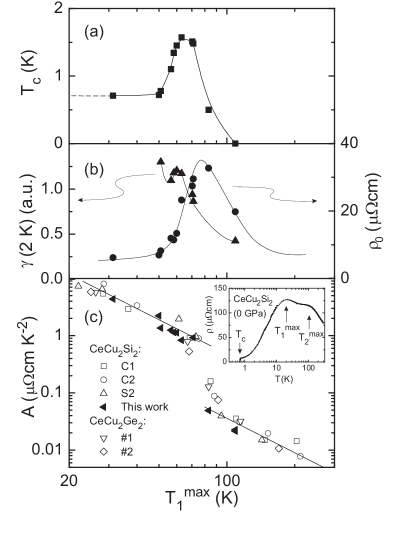
Figure 2: Plotted against $T_{1}^{\rm max}$ (defined in inset), a measure of the characteristic energy scale of the system, are (a) the bulk superconducting transition temperature, (b) the residual resistivity and $\gamma$ coefficient of the electronic specific heat, and (c) the coefficient $A$ of the $\rho\sim AT^{2}$ law of resistivity. Note the straight lines where the expected $A\propto(T_{1}^{\rm max})^{-2}$ scaling is followed. The maximum of $T_{\rm c}$ coincides with the start of the region where the scaling relation is broken, while the maximum in residual resistivity is situated in the middle of the collapse in $A$. Pressure increases towards the right-hand side of the scale (high $T_{\rm K}$). [18]

The huge peak of $\rho_{0}$ at around $P\sim P_{\rm v}$ can be understood as a many-body effect enhancing the impurity potential. In the forward scattering limit, this enhancement is proportional to the valence susceptibility $-(\partial n_{\rm f}/\partial\varepsilon_{\rm f})_{\mu}$, where $\varepsilon_{\rm f}$ is the atomic f-level of the Ce ion, and $\mu$ is the chemical potential [16]. Physically speaking, local valence change coupled to the impurity or disorder gives rise to the change of valence in a wide region around the impurity which then scatters the quasiparticles quite strongly, leading to the increase of $\rho_{0}$ (see Fig. 3). On the other hand, the effect of AF critical fluctuations on $\rho_{0}$ is rather moderate as discussed in ref. MN. Thus, the critical pressure $P_{\rm v}$ can be clearly defined by the maximum of $\rho_{0}$.

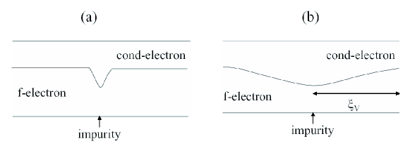
Figure 3: Schematic view of charge distribution of f- and conduction electrons around impurity: (a) at far from $P\sim P_{\rm v}$ where the effect of impurity remains as short-ranged so that the residual resistivity $\rho_{0}$ is not enhanced; (b) at around $P\sim P_{\rm v}$ where the effect of impurity extends to long-range region, because the correlation length $\xi_{\rm v}$ of valence fluctuations diverges as $P\rightarrow P_{\rm v}$, leading to highly enhanced $\rho_{0}$.

Other characteristic behaviors shown in Fig. 2 near $P=P_{\rm v}$ are peak of the $T_{\rm c}$ and the Sommerfeld coefficient $\gamma(T=2~{}{\rm K})$ at slightly lower pressure than $P_{\rm v}$. These behaviors can be understood on the basis of explicit theoretical calculations in which almost local valence fluctuations of Ce is shown to develop around the pressure where the sharp valence crossover occurs. [14, 17, 18, 62] Another characteristic behavior is that the $T$-linear behavior is observed in $[\rho(T)-\rho_{0}]$ over rather wide temperature range above $T_{\rm c}$. This also can be understood on the basis of a picture of the almost local CVF, [18] which is related to the issue discussed in §3.

Much more direct evidence for the sharp crossover of the valence of Ce ion in CeCu₂Si₂ was obtained by ⁶³Cu-NQR measurements at temperature down to $T=3.1\,$K and under pressures up to $P=5.5\,$GPa passing $P_{\rm v}\simeq 4.5\,$GPa. [63, 64, 65] Namely, the NQR frequency ${}^{63}\nu_{\rm Q}$ suddenly deviates at above 4 GPa from the linear $P$-dependence in the low pressure range ($P\leq 3.5\,$GPa). This sudden downward deviation of ${}^{63}\nu_{\rm Q}$ can be regarded as due to an increase of Ce valence, because the linear $P$-dependence is recovered again at $P>4.5\,$GPa. The $P$-dependence of the deviation in ${}^{63}\nu_{\rm Q}$ is shown in Fig. 4. Corresponding change of the valence $\Delta n_{\rm f}$ was estimated to be $\Delta n_{\rm f}=0.05$ by the first principles calculations, [65] which may give the change in $n_{\rm f}$, say from $n_{\rm f}=0.99$ to $n_{\rm f}=0.94$ corresponding to that of decrease of mass enhancement by one order of magnitude (two orders of magnitude in the $A$ coefficient of the resistivity).

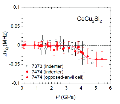
Figure 4: (Color online) Pressure dependence of deviation from the linear $P$ dependence of the NQR frequency ${}^{63}\nu_{\rm Q}$ in CeCu₂Si₂. [65]

It should be mentioned, however, that measurements of the X-ray powder diffraction (XRPD) at $T=12\,$K under presser (in CeCu₂Si₂) detected no sudden change in variations of lattice constant except for a very tiny change (of the same order as the experimental resolution) at around $P=4.5\,$GPa. [65] In ref. Kobayashi, it was also reported that the result of similar measurements in CeCu₂Ge₂ shows no detectable change in the volume at around $P=15\,$GPa in contrast to the report of ref. Onodera. The difference in two results was suggested to be due to that of pressure medium. Recent measurements of the X-ray absorption spectroscopy at Ce L3 edge at $T=14\,$K under high pressure in CeCu₂Si₂ also shows no discontinuous change at around $P=4.5\,$GPa, [67] which is not inconsistent with the result of XRPD in ref. Kobayashi. Origin of this discrepancy on valence change by two probes, NQR and X-ray, is not clear for the moment.

2.2 CeRhIn₅

CeRhIn₅ is a prototypical heavy fermion system in which superconductivity and antiferromagntic order coexist under pressure. [68, 69] The phase diagram is shown in Fig. 5: (a) in the $P$-$H$ plane at $T=0\,$K, and (b) in the $P$-$T$ plane at $H=0$. Measurements of de Haas-van Alphen (dHvA) effect have been performed along the arrow in Fig. 5(a), [71] revealing the following aspects: (1) the Fermi surfaces change at $P=P_{\rm c}$ from those expected for localized $f$ electrons (as in LaRhIn₅) to those for itinerant $f$ electrons. (2) the cyclotron mass exhibits a sharp peak at around $P=P_{\rm c}$. At $P=P_{\rm c}$, the AF order disappears suddenly, corresponding to the discontinuous change of the Fermi surfaces. It is mysterious that the effective mass of quasiparticles increases steeply towards $P=P_{\rm c}$ where the first order magnetic transition occurs.

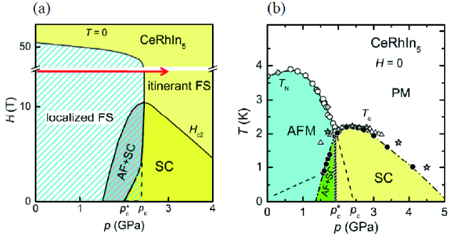
Figure 5: (Color online) (a) Phase diagram of CeRhIn₅ at $T\to 0$ K in $P$-$H$ plane. [68] (b) Phase diagram of CeRhIn₅ without magnetic field ($H=0$ Tesla) in $P$-$T$ plane. [68] The dashed line indicates the superconducting transition temperature reported in ref. Chen.

This problem was resolved by a theoretical analysis on the basis of the extended PAM, eq. (1), supplemented by the Zeeman term,

$$H_{\rm mag}=-h\sum_{i}(S^{\rm f}_{iz}+S^{\rm c}_{iz}),$$ (4)

where $h\equiv g\mu_{\rm B}H$. This Hamiltonian was treated by the mean-filed approximations both for the AF order and the slave boson which is introduced to take into account the strong local correlation effect between on-site $f$ electrons. [72, 73] Depending on the strength of the hybridization $V$ in the Hamiltonian, eq. (1), qualitative phase diagrams in the $P$-$T$ plane change as shown in Fig. 6. In the systems with relatively large $V$, the AF phase is suppressed so that $P_{\rm c}$, corrsponding to the AF-QCP, and $P_{\rm v}$, coresponding to the QCEP of valence transition or valence crossover, is well separated, as in CeCu₂(Si,Ge)₂ and Ce(Co,Ir)In₅ (Fig. 6(a)). In the systems with relatively weak $V$, the region of AF state extends to higher pressure region so that the intrinsic $P_{\rm c}$ becomes lager than $P_{\rm v}$. However, the AF order is cut by the valence crossover at $P=P_{\rm v}$ where AF order vanishes discontinuously, as in CeRhIn₅ (Fig. 6(c)). There occurs the case where $P_{\rm c}$ coincides with $P_{\rm v}$ at a certain strength of $V$ (Fig. 6(b)), giving a possible new type of quantum critical phenomena as in YbRh₂Si₂ [39].

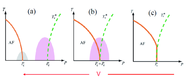
Figure 6: (Color online) Schematic $P$-$T$ Phase diagrams in $P$-$T$ plane for three cases corresponding to different strength of the hybridization $V$.

The results of microscopic calculations under the magnetic field $H$ for the case Fig. 6(c) are summarized as follows: [72]

1. Both lines of the first order valence transition and valence crossover almost coincides with that of AF transition of the first order; i.e., AF order is cut by the valence transition or valence crossover. [74]

2. Associated with the first order transition, the Fermi surface changes discontinuously from smaller size to larger size corresponding to the transition from a so-called “localized” $f$ electrons to “itinerant” ones.

3. The effective mass of quasiparticles exhibits a sharp peak structure around $P=P_{\rm c}$ as the band effect of folding or unfolding of the Fermi surface associated with the AF transition.

4. The effective mass of quasiparticles is already enhanced in the AF state from that given by the first-principles band structure calculations, implying that the hybridization between $f$ and conduction electrons is not vanishing there at all.

These results capture the essential experimental aspects of CeRhIn₅ obtained by dHvA experiments in ref. Shishido

Other experimental evidence for the valence crossover to be realized in CeRhIn₅ at $P=P_{\rm c}$ are the following three:

1. The resistivity at $T=2.25\,$K just above $T_{\rm c}$ exhibits huge peak at $P=P_{\rm c}$ [68, 75] as in the case of CeCu₂(Si,Ge)₂ as shown in Fig. 7(a). This strongly suggests that the valence fluctuations are growing sharply around $P=P_{\rm c}$ as discussed in ref. MM.

2. The exponent of $\alpha$, representing the $T$-dependence of $[\rho(T)-\rho_{0}]\propto T^{\alpha}$ approach $\alpha=1$ near $P=P_{\rm c}$ as demonstrated by Park et al. in ref. Park. This is also the signature of critical valence fluctuations. [18]

3. The Kadowaki-Wood scaling, $\sqrt{A}/m^{*}={\rm const}.$ or $A/\gamma^{2}={\rm const}.$, holds at $P\mathop{\vtop{\halign{#\cr$\hfil\displaystyle{<}\hfil$\crcr\kern 1.0pt\nointerlineskip\cr$\,\,\sim$ \crcr\kern 1.0pt\cr}}}\limits P_{\rm c}$, although both $A$ and $m^{*}$ grow steeply as $P$ approach $P_{\rm c}$ from lower pressure side as shown in Fig. 7(b). [68] This behavior cannot be understood from the scenario based on the AF criticality where $A/\gamma^{2}$ diverges.

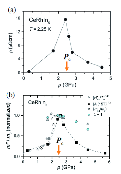
Figure 7: (Color online) (a) Enhanced resistivity at $T=T_{\rm c}$, (b) scaling of $\sqrt{A}$ and $m^{*}$ in CeRhIn₅.

Finally, we note that the pressure dependence of the SC transition temperature $T_{\rm c}$ and the upper critical field $H_{{\rm c}2}$ are quite different (see Fig. 5(a)). Namely, the former is almost flat at $P>P_{\rm c}$ while the latter prominently increases as $P_{\rm c}$ is approached from the higher pressure side. This suggests that the SC pairing interaction is promoted by the magnetic field $H$ itself. One of such possibility is that the QCEP of valence transition is located at the magnetic field $H=H^{*}$ ($>10\,$Tesla) on the phase boundary between AF and normal state in the phase diagram Fig. 5(a). This is not so ridiculous idea, considering that its phase boundary coincides with the valence crossover lines as mentioned in the item (1) above, [72] and the SC state is stabilized in the region where a sharp crossover of valence occurs. [14, 17, 18, 62]

3 Mode-Mode Coupling Theory for Critical Valence Fluctuations

In this section, we outline the theory for the critical exponents due to the critical valence fluctuations (CVF) shown in Table 1. [50] We start with the Hamiltonian (1) and construct the mode-mode coupling theory in parallel to the case of the theory for magnetic QCP which starts with the Hubbard model. [45, 47]

3.1 Formalism

In the model Hamiltonian (1), the on-site Coulomb repulsion $U_{\rm ff}$ between $f$ electrons is the strongest interaction, so that we first take into account its effect and after that construct the mode-mode coupling theory for critical valence fluctuations caused by the $f$-$c$ repulsion $U_{\rm fc}$. To consider the correlation effect due to $U_{\rm ff}$, we introduce the slave-boson operator $b_{i}$ to eliminate the doubly-occupied state, representing the effect of $U_{\rm ff}\to\infty$, under the constraint

$$\sum_{m}n^{\rm f}_{im}+Nb^{\dagger}_{i}b_{i}=1,$$ (5)

where $i$ indicates the site of $f$ electron, and $m$ represents the generalized spin labels extended from $\sigma=\uparrow,\downarrow$ to $m=1\cdots N$ for employing the large-$N$ expansion framework. [14]

The Lagrangian is written as ${\cal L}={\cal L}_{0}+{\cal L}^{\prime}$:

$${\cal L}_{0}=\sum_{{\bf k}m}c^{\dagger}_{{\bf k}m}\left(\partial_{\tau}+\bar{\varepsilon}_{\bf k}\right)c_{{\bf k}m}+\sum_{{\bf k}{\bf k^{\prime}}m}f^{\dagger}_{{\bf k}m}\left(\partial_{\tau}+\bar{\varepsilon}^{\rm f}_{{\bf k}-{\bf k^{\prime}}}\right)f_{{\bf k^{\prime}}m}$$

$$\qquad\qquad+\frac{V}{\sqrt{N_{\rm s}}}\sum_{{\bf k}{\bf k^{\prime}}m}\left(c^{\dagger}_{{\bf k}m}f_{{\bf k^{\prime}}m}b^{\dagger}_{{\bf k}-{\bf k^{\prime}}}+{\rm h.c.}\right)+\frac{N}{N_{\rm s}}\sum_{{\bf k}{\bf k^{\prime}}}b^{\dagger}_{\bf k}\lambda_{{\bf k}-{\bf k^{\prime}}}b_{\bf k^{\prime}}$$ (6)

$${\cal L^{\prime}}=-\frac{U_{\rm fc}}{N}\sum_{im}\left(n^{\rm c}_{im}+n^{\rm f}_{im}\right)+\frac{U_{\rm fc}}{N}\sum_{imm^{\prime}}n^{\rm f}_{im}n^{\rm c}_{im^{\prime}},$$ (7)

where $N_{\rm s}$ is the number of lattice sites, $\lambda_{\bf k}$ is the Lagrange multiplier to impose the constraint, and $\bar{\varepsilon}_{\bf k}\equiv\varepsilon_{\bf k}+\frac{U_{\rm fc}}{N}$ and $\bar{\varepsilon}^{\rm f}_{{\bf k}-{\bf k^{\prime}}}\equiv\left(\varepsilon_{\rm f}+\frac{U_{\rm fc}}{N}\right)\delta_{{\bf k}{\bf k^{\prime}}}+\frac{1}{\sqrt{N_{\rm s}}}\lambda_{{\bf k}-{\bf k^{\prime}}}$. Here, we have separated $\cal L$ as ${\cal L}_{0}$ and ${\cal L^{\prime}}$ to perform the expansion with respect to the $f$-$c$ Coulomb repulsion $U_{\rm fc}$.

For the term $\exp(-S_{0})$ with the action $S_{0}=\int_{0}^{\beta}d\tau{\cal L}_{0}(\tau)$, the saddle point solution is obtained via the stationary condition $\delta S_{0}=0$ by approximating spatially uniform and time independent ones, i.e., $\lambda_{\bf q}=\lambda\delta_{\bf q}$ and $b_{\bf q}=b\delta_{\bf q}$. The solution is obtained by solving mean-field equations $\partial S_{0}/\partial\lambda=0$ and $\partial S_{0}/\partial b=0$ self-consistently.

To make the action $S^{\prime}=\int_{0}^{\beta}d\tau{\cal L^{\prime}}(\tau),$ we introduce the identity applied by a Stratonovich-Hubbard transformation

$${\rm e}^{-S^{\prime}}=\int{\cal D}\varphi\,\exp\left[\sum_{im}\int_{0}^{\beta}d\tau\left\{-\frac{U_{\rm fc}}{2}\varphi_{im}(\tau)^{2}+{\rm i}\frac{U_{\rm fc}}{\sqrt{N}}\left(c_{im}f^{\dagger}_{im}-f_{im}c^{\dagger}_{im}\right)\varphi_{im}(\tau)\right\}\right].$$ (8)

Then, the partition function of the system is expressed as $Z=\int{\cal D}(cc^{\dagger}ff^{\dagger}\varphi)\exp(-S)$ with $S=S_{0}+S^{\prime}$. By performing Grassmann number integrals for $cc^{\dagger}$ and $ff^{\dagger}$, we obtain the action for the field $\varphi$ as (up to constant terms)

$$S\left[\varphi\right]=\sum_{m}\left[\frac{1}{2}\sum_{\bar{q}}\Omega_{2}(\bar{q})\varphi_{m}(\bar{q})\varphi_{m}(-\bar{q})\right.$$

$$\qquad\qquad+\left.\sum_{\bar{q}_{1},\bar{q}_{2},\bar{q}_{3}}\Omega_{3}(\bar{q}_{1},\bar{q}_{2},\bar{q}_{3})\varphi_{m}(\bar{q}_{1})\varphi_{m}(\bar{q}_{2})\varphi_{m}(\bar{q}_{3})\delta\left(\sum_{i=1}^{3}\bar{q}_{i}\right)\right.$$

$$\qquad\qquad+\left.\sum_{\bar{q}_{1},\bar{q}_{2},\bar{q}_{3},\bar{q}_{4}}\Omega_{4}(\bar{q}_{1},\bar{q}_{2},\bar{q}_{3},\bar{q}_{4})\times\varphi_{m}(\bar{q}_{1})\varphi_{m}(\bar{q}_{2})\varphi_{m}(\bar{q}_{3})\varphi_{m}(\bar{q}_{4})\delta\left(\sum_{i=1}^{4}\bar{q}_{i}\right)+\cdots\right].$$ (9)

Here, a dominant part of the coefficient of the quadratic term is given by

$$\Omega_{2}({\bf q},i\omega_{l})=U_{\rm fc}\left[1-\frac{2U_{\rm fc}}{N}\chi^{\rm ffcc}_{0}({\bf q},i\omega_{l})\right],$$ (10)

where

$$\chi^{\rm ffcc}_{0}({\bf q},i\omega_{l})\equiv-\frac{T}{N_{\rm s}}\sum_{{\bf k},n}G_{0}^{\rm ff}({\bf k}+{\bf q},i\varepsilon_{n}+i\omega_{l})G_{0}^{\rm cc}({\bf k},i\varepsilon_{n}),$$ (11)

where $G_{0}^{\rm ff}({\bf k},{\rm i}\varepsilon_{n})$ and $G_{0}^{\rm cc}({\bf k},{\rm i}\varepsilon_{n})$ are the Green function of $f$ and conduction electrons for the saddle point solution for $U_{\rm ff}=\infty$, respectively. [50]

Since long wave length $|{\bf q}|\ll q_{\rm c}$ around ${\bf q}={\bf 0}$ and low frequency $|{\omega}|\ll\omega_{\rm c}$ regions play dominant roles in critical phenomena, with $q_{\rm c}$ and $\omega_{\rm c}$ being cutoffs for momentum and frequency which are of the order of inverse of the lattice constant and the effective Fermi energy, respectively. Coefficients $\Omega_{i}$ for $i=2,3$, and 4 in eq. (9) are expanded for $q$ and $\omega$ around $({\bf 0},0)$ as follows: [50]

$$\Omega_{2}({\bf q},i\omega_{l})\approx\eta_{0}+Aq^{2}+C_{q}\left|\omega_{l}\right|,$$ (12)

where

$$\eta_{0}\equiv U_{\rm fc}\left[1-\frac{2U_{\rm fc}}{N}\chi^{\rm ffcc}_{0}({\bf 0},0)\right],$$ (13)

and

$$\Omega_{3}(q_{1},q_{2},q_{3})\approx\frac{v_{3}}{\sqrt{\beta N_{\rm s}}},\quad\Omega_{4}(q_{1},q_{2},q_{3},q_{4})\approx\frac{v_{4}}{\beta N_{\rm s}}.$$ (14)

We note that hereafter $A$ represents the coefficient of the $q^{2}$ term as in eq. (12), but not the coefficient of the $T^{2}$ term in the resistivity.

3.2 Renormalization group analysis

It is useful to analyze the property of the cubic and quartic terms in $\varphi$ in the action $S[\varphi]$, eq. (9), by the perturbation renormalization-group procedure: [47] (a) Integrating out high momentum and frequency parts for $q_{\rm c}/s<q<q_{\rm c}$ and $\omega_{\rm c}/s^{z}<\omega<\omega_{\rm c}$, respectively, with $s$ being a dimensionless scaling parameter $(s\geq 1)$ and $z$ the dynamical exponent. (b) Scaling of $q$ and $\omega$ by $q^{\prime}=sq$ and $\omega^{\prime}=s^{z}\omega$. (c) Re-scaling of $\varphi$ by $\varphi^{\prime}({\bf q^{\prime}},\omega^{\prime})=s^{a}\varphi({\bf q^{\prime}}/s,\omega^{\prime}/s)$. Then, we determine the scale factor $a$ so that the Gaussian term in eq. (9) becomes scale invariant, leading to $a=-(d+z+2)/2$ with $d$ being spatial dimension. Finally, the renormalization-group evolution for coupling constants $v_{j}$ ($j=3,\,4$) are given as

$$\frac{dv_{3}}{ds} = \left[6-(d+z)\right]v_{3}+{\cal O}(v_{3}^{2}),$$ (15)

$$\frac{dv_{4}}{ds} = \left[4-(d+z)\right]v_{4}+O(v_{4}^{2}).$$ (16)

By solving these equations, it is shown that higher order terms than the Gaussian term are irrelevant in the sense that

$$\lim_{s\to\infty}v_{j}(s)=0\ \ {\rm for}\ \ j\geq 3$$ (17)

for $d+z\geq 6$. This implies that the upper critical dimension $d_{\rm u}$ for the cubic term to be irrelevant is $d_{\rm u}=6$. In the case of pure three dimensional system ($d=3$) exhibiting valence change uniform in space, where $C_{q}=C/q$, dynamical exponent $z$ is given by $z=3$, i.e., $d+z=6=d_{\rm u}$, so that the cubic term is marginally irrelevant [62]. Hence, the universality class of the criticality of valence fluctuations belongs to the Gaussian fixed point. This implies that critical valence fluctuations are qualitatively described by the RPA framework with respect to $U_{\rm fc}$. The coefficient of the Gaussian term in eq. (9), i.e., eq. (12), is nothing but the inverse of the valence susceptibility $\Omega_{2}({\bf q},i\omega_{l})\equiv\chi_{\rm v}^{\rm RPA}({\bf q},i\omega_{l})^{-1}$. Namely, $\chi_{\rm v}^{\rm RPA}({\bf q},i\omega_{l})$ is given as

$$\chi_{\rm v}^{\rm RPA}(q,i\omega_{l})=\frac{1}{\eta_{0}+Aq^{2}+C_{q}|\omega_{l}|}.$$ (18)

However, there exist some cases with $z=2$ in general. For example, if the effect of non-magnetic impurity scattering is taken into account, $C_{q}$ is given as $C_{q}=C/{\rm max}\{q,l_{\rm i}^{-1}\}$ with $l_{\rm i}$ being the mean free path of impurity scattering, [13] leading to $z=2$ unless the effect of impurity scattering is neglected. Another one is the case where a valence change occurs as a density wave with a finite ordered wave vector, giving the dynamical exponent $z=2$ in general. Nevertheless, the cubic coefficient vanishes on the line which is extending from the first-order transition line to the crossover region, as discussed by Landau in the case of gas-liquid transition. [76] Namely, just at the QCEP of the valence transition, the cubic term is neglected safely, making the upper critical dimension of the system $d_{\rm u}=4$, but not $d_{\rm u}=6$, as far as the temperature dependence at the QCEP is concerned. Then, clean $(z=3)$ system and dirty $(z=2)$ system in three spatial dimension $(d=3)$ are both above the upper critical dimension, i.e., $d+z>d_{\rm u}=4$. Thus, the higher order terms other than the Gaussian term are irrelevant in the action, which makes the fixed point Gaussian.

3.3 Locality of CVF

With the use of the saddle point solution for $G_{0}^{\rm ff}({\bf k},{\rm i}\varepsilon_{n})$ and $G_{0}^{\rm cc}({\bf k},{\rm i}\varepsilon_{n})$, we have found that the coefficient $A$ in eq. (12) or eq. (18) is extremely small of the order of $q_{\rm c}^{-2}{\cal O}(10^{-2}$), or almost dispersionless critical valence fluctuation mode appears near $q=0$ not only for deep $\varepsilon_{\rm f}$, i.e., in the Kondo regime, but also for shallow $\varepsilon_{\rm f}$, i.e., in the mixed valence regime, because of strong on-site Coulomb repulsion for $f$ electrons in the extended PAM, eq. (1). [50]

The physical picture of emergence of this weak-$q$ dependence in the critical valence fluctuation is analyzed as follows: [62] The $q$-dependence in eq. (12) appears through $G_{0}^{\rm ff}({\bf k}+{\bf q},{\rm i}\varepsilon_{n})$ in $\chi_{0}^{\rm ffcc}({\bf q},,0)$, eq. (11). Near $q=0$, $\chi_{0}^{\rm ffcc}({\bf q},,0)$ is expanded as

$$\chi_{0}^{\rm ffcc}(q,0)=\chi_{0}^{\rm ffcc}(0,0)+\tilde{S}\left(\frac{V}{|\mu-\varepsilon_{\rm f}|}\right)^{2}q^{2},$$ (19)

where $\tilde{S}$ includes the effect of the f-electron self-energy for $U_{\rm ff}$ in eq. (1). Since the f-electron self-energy has almost no $q$ dependence in heavy electron systems, the $q$ dependence of the $f$-electron propagator $G_{0}^{\rm ff}({\bf k}+{\bf q})$ comes from the hybridization $V$ with conduction electrons with the dispersion $\varepsilon_{{\bf k}+{\bf q}}$, as seen in the coefficient of the $q^{2}$ term in eq. (19). Hence, the reduction of the coefficient $A$ in eq. (18) is caused by two factors. One is due to the smallness of $(V/|\mu-\varepsilon_{\rm f}|)^{2}$. In typical heavy electron systems, this factor is smaller than $10^{-1}$. The other one is the reduction of the coefficient $\tilde{S}$, which is suppressed by the effects of the on-site electron correlations $U_{\rm ff}$ in eq. (1). Numerical evaluations of $\chi_{0}^{\rm ffcc}(q,0)$ based on the saddle point solution for $U_{\rm ff}=\infty$ in eq. (1) show that extremely small $\tilde{S}$ appears not only in the Kondo regime, but also in the mixed-valence regime, [50] indicating that the reduction by $\tilde{S}$ plays a major role. These multiple reductions are the reason why extremely small coefficient $A$ appears in eq. (18).

The extremely small $A$ in eq. (12) or eq. (18) makes the characteristic temperature for critical valence fluctuations

$$T_{0}\equiv\frac{Aq_{\rm B}^{3}}{2\pi C}$$ (20)

extremely small. Here, $q_{\rm B}$ is a momentum at the Brillouin zone boundary. Hence, even at low enough temperature than the effective Fermi temperature of the system, i.e., so-called Kondo temperature, $T\ll T_{\rm K}$, the temperature scaled by $T_{0}$ can be very large: $t\equiv T/T_{0}\gg 1$. This is the main reason why unconventional criticality emerges at “low” temperatures, which will be explained below. For, YbRh₂Si₂, $T_{0}$ is estimated as $T_{0}=7$ mK using the band structure calculations. [77, 78] There are no available data for other systems shown in Table 1 for the moment.

3.4 Mode-mode coupling theory for CVF

Now, we construct a self-consistent renormalization (SCR) theory for valance fluctuations. Although higher order terms $v_{j}$ $(j\geq 3)$ in $S[\varphi]$ are irrelevant as shown above, the effect of their mode couplings renormalize $\eta_{0}$, inverse susceptibility in the RPA, and low-$T$ physical quantities significantly as is well known in spin-fluctuation theories. [45, 46, 47, 48] To construct the best Gaussian for $S[\varphi]$, we employ the so-called Feynman’s inequality on the free energy: [79]

$$F\leq F_{\rm eff}+T\langle S-S_{\rm eff}\rangle_{\rm eff}\equiv\tilde{F}(\eta),$$ (21)

where

$$S_{\rm eff}[\varphi]\equiv\frac{1}{2}\sum_{m}\sum_{{\bf q},{l}}(\eta+Aq^{2}+C_{q}|\omega_{l}|)|\varphi_{m}({\bf q},i\omega_{l})|^{2},$$ (22)

and $\eta$ is determined to make $\tilde{F}(\eta)$ be optimum. By optimal condition $d\tilde{F}(\eta)/d\eta=0$, the self-consistent equation for $\eta$, i.e., the SCR equation, is obtained as follows:

$$\eta=\eta_{0}+\frac{3v_{4}}{N_{\rm s}}T\sum_{{\bf q},l}(\eta+Aq^{2}+C_{q}|\omega_{l}|)^{-1}.$$ (23)

When the system is clean and the valence change is uniform in space, i.e., $C_{q}=C/q$, the SCR equation in $d=3$ in the $Aq_{\rm B}^{2}\mathop{\vtop{\halign{#\cr$\hfil\displaystyle{<}\hfil$\crcr\kern 1.0pt\nointerlineskip\cr$\,\,\sim$ \crcr\kern 1.0pt\cr}}}\limits\eta$ regime with $q_{\rm B}$ being the momentum at the Brillouin Zone is given by

$$y=y_{0}+\frac{3}{2}y_{1}t\left[\frac{x_{\rm c}^{3}}{6y}-\frac{1}{2y}\int_{0}^{x_{\rm c}}dx\frac{x^{3}}{x+\frac{t}{6y}}\right],$$ (24)

where $y\equiv\eta/(Aq_{\rm B}^{2})$, $x\equiv q/q_{\rm B}$, $x_{\rm c}\equiv=q_{\rm c}/q_{\rm B}$, and $y_{0}$ parameterizes a distance from the criticality and $y_{1}$ is a dimensionless mode-coupling constant of $O(1)$. The solution of Eq. (24) is quite different from that of ordinary SCR equation for spin fluctutions [45] because of extreme smallness of $A$ in eq. (18).

In the $y\gg t$ limit at QCEP with $y_{0}=0$,an analytic solution of eq. (24) is obtained as $\chi_{\rm v}(0,0)=y^{-1}\sim t^{-2/3}$ for both the clean $(z=3)$ system and dirty $(z=2)$ system. This indicates that the valence susceptibility shows unconventional criticality

$$\chi_{\rm v}({\bf 0},0)=\eta^{-1}\propto t^{-2/3}.$$ (25)

Figure 8(a) shows numerical solutions of Eq. (24) for a series of value $y_{0}$’s. As discussed above, the region of $t\equiv T/T_{0}$ shown in Fig. 8 corresponds to that of $T\ll T_{\rm F}\sim O(D)$, so that a wide range of $t=T/T_{0}$ is shown in the plot even though near the criticality $y\ll 1$. The least square fit of the data for $5\leq t\leq 100$ gives $y\propto t^{0.551}$. If we express the inverse susceptibility $y$ as $y\propto t^{-\zeta}$, the exponent $\zeta$ has a temperature dependence and $0.5\mathop{\vtop{\halign{#\cr$\hfil\displaystyle{<}\hfil$\crcr\kern 1.0pt\nointerlineskip\cr$\,\,\sim$ \crcr\kern 1.0pt\cr}}}\limits\zeta\mathop{\vtop{\halign{#\cr$\hfil\displaystyle{<}\hfil$\crcr\kern 1.0pt\nointerlineskip\cr$\,\,\sim$ \crcr\kern 1.0pt\cr}}}\limits 0.7$ depending on the temperature range.

On the other hand, in the region of extremely low temperatures, $t=T/T_{0}\ll 1$, the solution is given by the conventional one with $d=3$ and $z=3$, i.e., $y(t)\propto t^{4/3}$, coinciding with that in three dimensional ferromagnetic QCP. In the dirty system, with $d=3$ and $z=2$, the asymptotic form is given as $y(t)\propto t^{3/2}$, coinciding with that in three dimensional AF QCP.

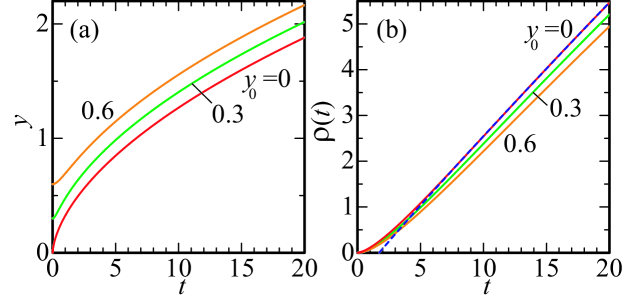
Figure 8: (Color online) (a) Numerical solutions of eq. (1) for $y_{0}=0.0$ (at QCP), 0.3, and 0.6 at $y_{1}=1$ and $x_{\rm c}=1$. (b) Electrical resistivity $\rho(T)$ calculated by using $y(t)$ in (a). Dashed line represents the linear-$t$ fit.

3.5 Critical exponents of physical quantities

The next problem is how this new type of criticality is manifested in physical quantities listed in Table 1. It is important to note that the valence fluctuation propagator $\chi_{\rm v}({\bf q},i\omega_{l})$ is qualitatively given by that of RPA as discussed above. A crucial consequence of this fact is that the dynamical $f$-spin susceptibility

$$\chi_{\rm f}^{+-}({\bf q},i\omega_{l})\equiv\int_{0}^{\beta}d\tau\langle T_{\tau}S_{\rm f}^{+}({\bf q},\tau)S_{\rm f}^{-}({\bf-q},0)\rangle{\rm e}^{i\omega_{l}\tau}$$ (26)

has the same structure as $\chi_{\rm v}$ in the RPA framework as shown in Fig. 9. At the QCEP of the valence transition, the valence susceptibility $\chi_{\rm v}({\bf 0},0)$ diverges. The common structure indicates that $\chi_{\rm f}^{+-}({\bf 0},0)$ also diverges at the QCEP. Then, the singularity in the uniform spin susceptibility $\chi(T)$ is given by

$$\chi\approx\chi^{\rm f}_{\rm s}\approx\frac{3}{2}\mu_{\rm B}^{2}g_{\rm f}^{2}\chi^{+-}_{\rm f}({\bf 0},0)\propto\chi_{\rm v}(0,0),$$ (27)

where $\chi^{\rm f}_{\rm s}$ is the uniform $f$-spin susceptibility, $\mu_{\rm B}$ the Bohr magneton, and $g_{\rm f}$ Lande’s g factor for $f$ electrons. This gives a qualitative explanation for the fact that the uniform spin susceptibility diverges at the QCEP of valence transition under the magnetic field, which was verified by the slave-boson mean-field theory applied to the extended PAM, Eq. (1). [80, 81] Numerical calculations for the model (1) in $d=1$ by the DMRG [80] and in $d=\infty$ by the DMFT [34] also show the simultaneous divergence of $\chi_{\rm v}$ and uniform spin susceptibility under the magnetic field, again reinforcing the above argument based on RPA.

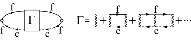
Figure 9: Feynman diagrams for dynamical valence susceptibility and dynamical spin susceptibility for f electrons. Solid lines and dashed lines represent the f- and conduction-electron Green functions, $G^{\rm ff}_{0}$ and $G^{\rm cc}_{0}$, respectively. Wiggly lines represent $U_{\rm fc}$.

Therefore, the uniform magnetic susceptibility $\chi(T)$ is proportional to the valence susceptibility $\chi_{\rm v}({\bf 0},0)$ and exhibits the same critical behavior as $\chi(T)\propto t^{-\zeta}$ at QCEP of valence transition. The spin-lattice relaxation rate $1/{(T_{1}T)}$ has the same singularity in the limit $T\to 0$ as the uniform susceptibility $\chi(T)$ in the case of $d=3$ and $z=3$: i.e., $1/T_{1}T\propto t^{-\zeta}$. Therefore, for the region $y\gg t$, $\chi(t)\sim t^{-2/3}$ and $(T_{1}T)^{-1}\sim t^{-2/3}$. When $T$ is decreased down to $T\sim T_{0}$, $y$ in eq. (24) is evaluated as $y\sim t^{0.5}$ by the least square fit of the numerical solution. Hence, depending on the flatness of critical valence fluctuation mode and measured temperature range, $\chi(T)\sim t^{-\zeta}$ and $(T_{1}T)^{-1}\sim t^{-\zeta}$ with $0.5\mathop{\vtop{\halign{#\cr$\hfil\displaystyle{<}\hfil$\crcr\kern 1.0pt\nointerlineskip\cr$\,\,\sim$ \crcr\kern 1.0pt\cr}}}\limits\zeta\mathop{\vtop{\halign{#\cr$\hfil\displaystyle{<}\hfil$\crcr\kern 1.0pt\nointerlineskip\cr$\,\,\sim$ \crcr\kern 1.0pt\cr}}}\limits 0.7$ are predicted as shown in Table 1 in which good agreement with experiments is manifested.

The electrical resistivity $\rho(T)$ is calculated following a procedure used in the case of critical spin fluctuation as follows: [82]

$$\rho(T)\propto\frac{1}{T}\int_{-\infty}^{\infty}d\omega\omega n(\omega)[n(\omega)+1]\int_{0}^{q_{\rm c}}dqq^{3}{\rm Im}\chi_{\rm v}^{\rm R}(q,\omega),$$ (28)

where $n(\omega)=1/({\rm e}^{\beta\omega}-1)$ is the Bose distribution function, and $\chi_{\rm v}^{\rm R}(q,\omega)=(\eta+Aq^{2}-iC_{q}\omega)^{-1}$, the retarded valence susceptibility. As for $\eta=y(t)(Aq_{\rm B}^{2})$, $y(t)$ shown in Fig. 8(a) is used for the clean system $C_{q}=C/q$. The temperature dependence is shown in Fig. 8(b) where the normalization constant is taken as unity. In the region $y\mathop{\vtop{\halign{#\cr$\hfil\displaystyle{>}\hfil$\crcr\kern 1.0pt\nointerlineskip\cr$\,\sim$ \crcr\kern 1.0pt\cr}}}\limits t$ (but $T\ll T_{\rm K}$), $\rho(t)\propto t$. This behavior arises from the high-temperature limit of Bose distribution function, indicating that the system is described as if it is in the classical regime, because the system is in the high-$T$ regime in the scaled temperature $t\equiv T/T_{0}\gg 1$, in spite of $T\ll T_{\rm K}$. The emergence of $\rho(t)\propto t$ behavior can be understood from the locality of valence fluctuations: In the system with an extremely small coefficient $A$ the dynamical exponent is regarded as almost $z=\infty$ when we write $C_{q}$ in a general form as $C_{q}=C/q^{z-2}$. If we use this expression ($A=0$ corresponding to $z=\infty$) in $\chi_{\rm v}^{\rm R}(q,\omega)$ in the calculation of $\rho(T)$ , we easily obtain $\rho(T)\propto T$ toward $T\to 0$ K. This result indicates that the locality of valence fluctuations causes the $T$-linear resistivity. Indeed, the emergence of $\rho(T)\propto T$ by valence fluctuations was shown theoretically on the basis of the valence susceptibility $\chi_{\rm v}$ which has an approximated form for $z=\infty$ in Ref. Holmes.

On the other hand, in the region $t=T/T_{0}\ll 1$, the resistivity behaves as $\rho\sim t^{5/3}$ in the clean system and $\rho\sim t^{3/2}$ in the dirty system in the $t\to 0$ limit $(T\ll T_{0}\ll T_{\rm K})$. Therefore, the temperature dependence is expected to crossover at $T=T_{0}$. Indeed, such a crossover has been observed in $\beta$-YbAlB₄ as shown in Table 1.

The specific heat $C(T)$ is estimated through the effect of self-energy of quasiparticles due to an exchange of valence-fluctuation modes given by (18). [18, 83] A numerical solution of the self-energy gives a logarithmic temperature dependence in the specific-heat coefficient $C/T\propto-{\log}t$ in a certain temperature range $T\ll T_{0}$. The logarithmic $t$ dependence can remain even in a range $T>T_{0}$, where the uniform magnetic susceptibility and the resistivity behave as $\chi(t)\sim t^{-\zeta}$ with $0.5\mathop{\vtop{\halign{#\cr$\hfil\displaystyle{<}\hfil$\crcr\kern 1.0pt\nointerlineskip\cr$\,\,\sim$ \crcr\kern 1.0pt\cr}}}\limits\zeta\mathop{\vtop{\halign{#\cr$\hfil\displaystyle{<}\hfil$\crcr\kern 1.0pt\nointerlineskip\cr$\,\,\sim$ \crcr\kern 1.0pt\cr}}}\limits 0.7$ and $\rho(t)\sim t$, respectively. On the other hand, it is also possible that, in the case of the local limit $A\approx 0$, the power law behavior $C/t\propto\chi_{\rm v}(0,0)\propto t^{-\zeta}$ appears [18] before the conventional logarithmic behavior at high temperature region $T\mathop{\vtop{\halign{#\cr$\hfil\displaystyle{<}\hfil$\crcr\kern 1.0pt\nointerlineskip\cr$\,\,\sim$ \crcr\kern 1.0pt\cr}}}\limits T_{\rm K}$, which is usually observed in heavy fermion metal such as CeCu₆, [84] sets in.

In conclusion of this section, when experimentally accessible lowest temperature is larger than $T_{0}$, unconventional criticality dominates all the physical quantities down to the lowest temperature, reproducing the unconventional criticality summarized in Table 1.

4 Perspective

The results on unconventional criticality due to the CVF succeeded in explaining existing experimental aspects coherently as discussed in §3. On the other hand, the absolute value of change in the valence predicted by the theory on the extended PAM is larger than that observed in experiments in general. This originates from an inevitable problem of the Anderson model. In the PAM, original one or extended one, the conduction electrons which hybridize with localized $f$ electron have the same local symmetry, namely the same CEF symmetry, around the Ce- or Yb-site. Therefore, when one measures the valence, say by Ce L₃ edge absorption, electrons with the local CEF symmetry would be counted together. Namely, a part of “conduction electrons” (in the Anderson model) would be regarded as electrons with $f$-symmetry, or the $f$-electron state measured by X-ray is the hybridized object of $f$- and conduction electrons on ligands. Conduction electrons with a certain CEF symmetry at one site can mix with component of conduction electron with another CEF symmetry at different (say adjacent) sites. This kind of effect is out of scope of our extended PAM. Therefore, the decrement of valence measured by experiments would be far smaller than that predicted by theory based on our extended PAM. A more realistic model including such an effect is desired. Nevertheless, the model Hamiltonian, (1), is useful as the “fixed-point” model Hamiltonian which describes the critical behaviors associated with the critical valence transition.

A related problem is how to take into account the effect of $f$-electron state in the excited CEF levels. In our model, (1), we have neglected effects of excited CEF levels. For the moment, it is not so clear whether those CEF states give an essential effect in the case of a realistic CEF level scheme measured by the neutron scattering experiment, [85] while the effect of charge transfer of $f$ electrons between ground and excited CEF levels has been discussed by Hattori [86] on the basis of a CEF level scheme which is practically different from the observed one. In any case, such effects certainly deserve further investigations.

Recently, a series of anomalies have been observed in transport properties of CeCu₂Si₂ [87, 88] and $\beta$-YbAlB₄ [89]. Quite recently, it turned out that the CVF can give rise to an effect in the Hall conductivity and the Hall coefficient. It is also expected that the Seebeck effect and the Nernst effect are greatly influenced by the CVF.

References

- [1] F. Steglich, J. Aarts, C. D. Bredl, W. Lieke, D. Meschede, and W. Franz, and H. Schäfer: Phys. Rev. Lett. 43 (1979) 1892.
- [2] O. Stockert, J. Arndt, E. Faulhaber, C. Geibel, H. S. Jeevan, S. Kirchner, M. Loewenhaupt, K. Schmalzl, W. Schmidt, Q. Si, and F. Steglich: Nature Physics 7 (2011) 119.
- [3] F. M. Grosche, S. R. Julian, N. D. Mathur, and G. G. Lonzarich: Physica B 223/224 (1996) 50.
- [4] N. D. Mathur, F. M. Grosche, S. R. Julian, I. R. Walker, D. M. Freye, R. K. W. Haselwimmer, and G. G. Lonzarich: Nature 394 (1998) 39.
- [5] R. Movshovich, T. Graf, D. Mandrus, J. D. Thompson, J. L. Smith, and Z. Fisk: Phys. Rev. B 53 (1996) 8241.
- [6] K. Miyake, S. Schmitt-Rink, and C. M. Varma: Phys. Rev. B 34 (1986) 6554.
- [7] D. J. Scalapino, E. Loh, Jr., and J. E. Hirsch: Phys. Rev. B 34 (1986) 8190.
- [8] P. Monthoux and G. G. Lonzarich: Phys. Rev. B 63 (2001) 054529.
- [9] T. Moriya and K. Ueda: Adv. Phys. 49 (2000) 555.
- [10] B. Bellarbi, A. Benoit, D. Jaccard, J. M. Mignot, and H. F. Braun: Phys. Rev. B 30 (1984) 1182.
- [11] H. Razafimandimby, P. Fulde, and J. Keller: Z. Phys. 54 (1984) 111.
- [12] D. Jaccard, H. Wilhelm, K. Alami-Yadri, and E. Vargoz: Physica B 259-261 (1999) 1.
- [13] K. Miyake, O. Narikiyo, and Y. Onishi: Physica B 259-261 (1999) 676.
- [14] Y. Onishi and K. Miyake: J. Phys. Soc. Jpn. 69 (2000) 3955.
- [15] Y. Onishi and K. Miyake: Physica B 281&282 (2000) 191.
- [16] K. Miyake and H. Maebashi: J. Phys. Soc. Jpn. 71 (2002) 1007.
- [17] S. Watanabe, M. Imada, and K. Miyake: J. Phys. Soc. Jpn. 75 (2006) 043710.
- [18] A. T. Holmes, D. Jaccard, and K. Miyake: Phys. Rev. B 69 (2004) 024508.
- [19] H. Q. Yuan, F. M. Grosche, M. Deppe, C. Geibel, G. Sparn, and F. Steglich: Science 302 (2003) 2104.
- [20] S. Doniach: Physica B 91 (1977) 231.
- [21] See for example, D. C. Koskenmaki and K. A. Geschneidner: Handbook on the Physics and Chemistry of the Rare Earths, edited by K. A. Qschneidner and L. Eyring (North-Holland, Amsterdam, 1978), Vol. 1, Chap. 4.
- [22] B. Coqblin and A. Blandin: Adv. Phys. 17 (1968) 281.
- [23] J. W. Allen and R. M. Martin: Phys. Rev. Lett. 49 (1982) 1106.
- [24] M. Dzero, M. R. Norman, I. Paul, C. Pépin, and J. Schmalian: Phys. Rev. Lett. 97 (2006) 185701.
- [25] L. M. Falicov and J. C. Kimball: Phys. Rev. Lett. 22 (1969) 997.
- [26] C. M. Varma: Rev. Mod. Phys. 48 (1976) 219.
- [27] A. C. Hewson and P. S. Riseborough: Solid State Commun. 22 (1977) 379.
- [28] P. Schlottmann: Phys. Rev. B 22 (1980) 613.
- [29] T. A. Costi and A. C. Hewson: Physica C 185-189 (1991) 2649.
- [30] R. Takayama and O. Sakai: J. Phys. Soc. Jpn. 66 (1997) 1512.
- [31] I. E. Perakis and C. M. Varma: Phys. Rev. B 49 (1994) 9041.
- [32] D. I. Khomskii and A. N. Kocharjan: Solid State Commun. 18 (1976) 985.
- [33] Y. Saiga, T. Sugibayashi, and D. S. Hirashima: J. Phys. Soc. Jpn. 77 (2008) 114710.
- [34] T. Sugibayashi, A. Tsuruta, and K. Miyake: Physica C 470 (2010) S550.
- [35] K. Kubo: J. Phys. Soc. Jpn. 80 (2011) 114711.
- [36] I. Hagymasi, K. Itai, and J. Solyom: Acta Phys. Pol. A 121 (2012) 1070.
- [37] E. Bauer, R. Hauser, L. Keller, P. Fischer, O. Trovarelli, J. G. Sereni, J. J. Rieger, and G. R. Stewart: Phys. Rev. B 56 (1997) 711.
- [38] C. Seuring, K. Heuser, E.-W Scheidt, T. Schreiner, E. Bauer, and G. R. Stewart: Physica B 281-282 (2000) 374.
- [39] O. Trovarelli, C. Geibel, S. Mederle, C. Langhammer, F.M. Grosche, P. Gegenwart, M. Lang, G. Sparn, and F. Steglich: Phys. Rev. Lett. 85 (2000) 626.
- [40] K. Ishida, K. Okamoto, Y. Kawasaki, Y. Kitaoka, O. Trovarelli, C. Geibel, and F. Steglich: Phys. Rev. Lett. 89 (2002) 107202.
- [41] H. v. Löhneysen, A. Rosch, M. Vojta, and P. Wölfle: Rev. Mode. Phys. 79 (2007) 1015.
- [42] S. Nakatsuji, K. Kuga, Y. Machida, T. Tayama, T. Sakakibara, Y. Karaki, H. Ishimoto, S. Yonezawa, Y. Maeno, E. Pearson, G. G. Lonzarich, L. Balicas, H. Lee, and Z. Fisk: Nature Phys. 4 (2008) 603.
- [43] Y. Matsumoto, S. Nakatsuji, K. Kuga, Y. Karaki, N. Horie, Y. Shimura, T. Sakakibara, A. H. Nevidomskyy, and P. Coleman: Science 331 (2011) 316.
- [44] K. Deguchi, S. Matsukawa, N. K. Sato, T. Hattori, K. Ishida, H. Takakura, and T. Ishimasa: Nature Mat. 11 (2012) 1013.
- [45] T. Moriya : Spin Fluctuations in Itinerant Electron Magnetism (Springer, Berlin, 1985).
- [46] T. Moriya and T. Takimoto: J. Phys. Soc. Jpn. 64 (1995) 960.
- [47] J. A. Hertz: Phys. Rev. B 14 (1976) 1165.
- [48] A. J. Millis: Phys. Rev. B 48 (1993) 7183.
- [49] M. Hatatani, O. Narikiyo and K. Miyake FJ. Phys. Soc. Jpn. 67 (1998) 4002; M. Hatatani, PhD Thesis, 2000, Graduate School of Engineering Science, Osaka University.
- [50] S. Watanabe and K. Miyake, Phys. Rev. Lett. 105 (2010) 186403.
- [51] S. Watanabe and K. Miyake, J. Phys.: Condens. Matter 24 (2012) 294208.
- [52] Q. Si, S. Rabello, K. Ingersent, and J. L. Smith: Nature 413 (2001) 804.
- [53] P. Coleman C. Pépin, Q. Si, and R. Ramazashvili: J. Phys.: Condens. Matter 13 (2001) R723.
- [54] Q. Si: Physica B 378-380 (2006) 23.
- [55] T. Misawa, Y. Yamaji, and M. Imada: J. Phys. Soc. Jpn. 78 (2009) 084707.
- [56] A. Ramires, P. Coleman, A. H. Nevidomskyy, and A. M. Tsvelik: Phys. Rev. Lett. 109 (2012) 176404.
- [57] T. M. Rice and K. Ueda: Phys. Rev. B 34 (1986) 6420.
- [58] H. Shiba: J. Phys. Soc. Jpn. 55 (1986) 2765.
- [59] K. Kadowaki and S. B. Woods: Solid State Commun. 58 (1986) 507.
- [60] K. Miyake, T. Matsuura, and C. M. Varma: Solid State Commun. 71 (1989) 1149.
- [61] K. Miyake and O. Narikiyo: J. Phys. Soc. Jpn. 71 (2002) 867.
- [62] K. Miyake: J. Phys.: Condens. Matter 19 (2007) 125201.
- [63] K. Fujiwara, Y. Hata, K. Kobayashi, K. Miyoshi, J. Takeuchi, Y. Shimaoka, H. Kotegawa, T. C. Kobayashi, C. Geibel, and F. Steglich: J. Phys. Soc. Jpn. 77 (2008) 123711.
- [64] K. Fujiwara, M. Iwata, Y. Okazaki, Y. Ikeda, S. Araki, T. C. Kobayashi, K. Murata, C. Geibel, and F. Steglich: J. Phys.: Conf. Ser. 391 (2012) 012012.
- [65] T. C. Kobayashi, K. Fujiwara, K. Takeda, H. Harima, Y. Ikeda, T. Adachi, Y. Ohishi, C. Geibel, and F. Steglich: J. Phys. Soc. Jpn. 82 (2013) 114701.
- [66] A. Onodera, S. Tsuduki, Y. Ohishi, T. Watanuki, K. Ishida, Y. Kitaoka, and Y. Ōnuki: Solid State Commun. 123 (2002) 113.
- [67] J.-P. Rueff, S. Raymond, M. Taguchi, M. Sikora, J.-P. Itié, F. Baudelet, D. Braithwaite, G. Knebel, and D. Jaccard: Phys. Rev. Lett. 106 (2011) 186405.
- [68] G. Knebel, D. Aoki, J.-P. Brison, and J. Flouquet: J. Phys. Soc. Jpn. 77 (2008) 114704.
- [69] T. Park, V. A. Sidorov, F. Ronning, J.-X. Zhu, Y. Tokiwa, H. Lee, E. D. Bauer, R. Movshovich, J. L. Sarrao, and J. D. Thompson: Nature 456 (2008) 366.
- [70] G. F. Chen, K. Matsubayashi, S. Ban, K. Deguchi, and N. K. Sato: Phys. Rev. Lett. 97 (2006) 017005.
- [71] H. Shishido, R. Settai, H. Harima, and Y. Ōnuki: J. Phys. Soc. Jpn. 74 (2005) 1103.
- [72] S. Watanabe and K. Miyake: J. Phys. Soc. Jpn. 79 (2010) 033707.
- [73] S. Watanabe and K. Miyake, J. Phys.: Condens. Matter 23 (2011) 094217.
- [74] The result of the first-order AF transition is obtained for the band structure for branch in CeRhIn5 by the slave-boson mean-field calculation. It is noted that the order of the AF transition (as a consequence of ) is considered to depend on the detail of the parameter set of the extended PAM and calculation scheme.
- [75] T. Muramatsu, N. Tateiwa, T. C. Kobayashi, K. Shimizu, K. Amaya, D. Aoki, H. Shishido, Y. Haga, and Y. Ōnuki: J. Phys. Soc. Jpn. 70 (2001) 3362.
- [76] L. D. Landau: Zh. Exp. Teor. Fiz. 7 (1937) 19; ibid. 627; L. D. Landau: Collected papers of L. D. Landau, (Pergamon Press, Oxford, 1965) p. 193; L. D. Landau and E. M. Lifshitz: Statistical Physics, (Pergamon Press, London-Paris, 1958) 1st edition, §116 and §135.
- [77] M. R. Norman: Phys. Rev. B 71 (2005) 22045R.
- [78] T. Jeong and W. E. Pickett: J. Phys.: Condens. Matter 18 (2006) 6289.
- [79] R. Feynman: Statistical Mechanics: A Set Of Lectures (Advanced Books Classics).
- [80] S. Watanabe, A. Tsuruta, K. Miyake and J. Flouquet: Phys. Rev. Lett. 100 (2008) 236401.
- [81] S. Watanabe, A. Tsuruta, K. Miyake and J. Flouquet: J. Phys. Soc. Jpn. 78 (2009) 104706.
- [82] K. Ueda and T. Moriya: J. Phys. Soc. Jpn. 39 (1975) 605.
- [83] S. Watanabe and K. Miyake: arXiv:0906.3986
- [84] K. Satoh, T. Fujita, Y. Maeno, Y. Ōnuki, and T. Komatsubara: J. Phys. Soc. Jpn. 58 (1989) 1012.
- [85] S. Horn, E. Holland-Moritz, M. Loewenhaupt, F. Steglich, H. Scheuer, A. Benoit, and J. Flouquet: Phys. Rev. B 23 (1981) 3171.
- [86] K. Hattori: J. Phys. Soc. Jpn. 79 (2010) 114717.
- [87] G. Seyfarth, A.-S. Rüetschi, K. Sengupta, A. Georges, D. Jaccard, S. Watanabe, and K. Miyake: Phys. Rev. B 85 (2012) 205105.
- [88] S. Araki, Y. Shiroyama, Y. Ikeda, T. C. Kobayashi, S. Seiro, C. Geibel, and F. Steglich: J. Phys. Soc. Jpn. 80 (2011) SA061; private communications.
- [89] E. C. T. O fFarrell, Y. Matsumoto, and S. Nakatsuji: Phys. Rev. Lett. 109 (2012) 176405.