Herschel observations of EXtra-Ordinary Sources: ANALYSIS OF THE HIFI 1.2 THz WIDE SPECTRAL SURVEY TOWARD ORION KL I. METHODS

Abstract

We present a comprehensive analysis of a broad band spectral line survey of the Orion Kleinmann-Low nebula (Orion KL), one of the most chemically rich regions in the Galaxy, using the HIFI instrument on board the Herschel Space Observatory. This survey spans a frequency range from 480 to 1907 GHz at a resolution of 1.1 MHz. These observations thus encompass the largest spectral coverage ever obtained toward this high-mass star-forming region in the sub-mm with high spectral resolution, and include frequencies $>$ 1 THz where the Earth’s atmosphere prevents observations from the ground. In all, we detect emission from 39 molecules (79 isotopologues). Combining this dataset with ground based mm spectroscopy obtained with the IRAM 30 m telescope, we model the molecular emission from the mm to the far-IR using the XCLASS program which assumes local thermodynamic equilibrium (LTE). Several molecules are also modeled with the MADEX non-LTE code. Because of the wide frequency coverage, our models are constrained by transitions over an unprecedented range in excitation energy. A reduced $\chi^{2}$ analysis indicates that models for most species reproduce the observed emission well. In particular, most complex organics are well fit by LTE implying gas densities are high ($>$ 10⁶ cm^-3) and excitation temperatures and column densities are well constrained. Molecular abundances are computed using H₂ column densities also derived from the HIFI survey. The distribution of rotation temperatures, $T_{\rm rot}$, for molecules detected toward the hot core is significantly wider than the compact ridge, plateau, and extended ridge $T_{\rm rot}$ distributions, indicating the hot core has the most complex thermal structure.

1 Introduction

The origin of chemical complexity in the interstellar medium (ISM) is still not well understood. Approximately 175 molecules, not counting isotopologues, have been detected in the ISM (Menten & Wyrowski, 2011). The majority of complex molecules are thought to originate on grain surfaces although it is possible that gas-phase processes play a significant but, as of yet, unknown role (Herbst & van Dishoeck, 2009). One of the best ways to probe the chemistry that is occurring within the ISM is via unbiased spectral line surveys of star-forming regions in the mm and sub-mm, where molecular line emission is strong. High mass star-forming regions are among the most prolific emitters of complex organic molecules, which are produced primarily by energetic protostars that heat the surrounding material liberating molecules from dust grains and driving chemical reactions that cannot occur at lower temperatures (see e.g. Herbst & van Dishoeck, 2009; Garrod & Herbst, 2006; Garrod et al., 2008, and references therein). Unbiased spectral line surveys offer a unique avenue to explore the full chemical inventory and active molecular pathways in the dense ISM. Molecular rotational emissions are, for the most part, concentrated at mm and sub-mm wavelengths but the interference of atmospheric absorption has left broad wavelength regimes unexplored which has hampered our ability to obtain a complete view of the molecular content in these regions.

In this study, we present a comprehensive full band analysis of the HIFI 1.2 THz wide spectral survey toward the Orion Kleinmann-Low nebula (Orion KL), one of the archetypal massive star-forming regions in our Galaxy. Specifically, we model the emission in order to obtain reliable molecular abundances. Because of its close distance (420 pc; Menten et al., 2007; Hirota et al., 2007) and high luminosity ($\sim$ 10⁵ L_☉; Wynn-Williams et al., 1984), Orion KL has been exhaustively studied not only in the (sub-)mm but throughout the electromagnetic spectrum (Genzel & Stutzki, 1989; O’dell, 2001). As such, numerous high spectral resolution single dish line surveys have been carried out toward Orion KL in the mm (Johansson et al., 1984; Sutton et al., 1985; Blake et al., 1987; Turner, 1989; Greaves & White, 1991; Ziurys & McGonagle, 1993; Lee et al., 2001; Lee & Cho, 2002; Goddi et al., 2009b; Tercero et al., 2010, 2011), sub-mm (Jewell et al., 1989; Schilke et al., 1997, 2001; White et al., 2003; Comito et al., 2005; Olofsson et al., 2007; Persson et al., 2007), and far-IR (Lerate et al., 2006), though the far-IR survey was obtained at a much lower spectral resolution ($\nu/\Delta\nu$ $<$ 10⁴) than the (sub-)mm surveys ($\nu/\Delta\nu$ $>$ 10⁵). These studies show that Orion KL is one of the most chemically rich sources in the Milky Way and that the molecular line emission originates from several spatial/velocity components representing a diverse set of environments within Orion KL. Although not spatially resolved by single dish observations, these components can be differentiated using high resolution spectroscopy because they have significantly different line widths and central velocities. Furthermore, interferometric observations have mapped the spatial distributions of these components using different molecular tracers revealing a complex morphology (see e.g. Blake et al., 1996; Wright et al., 1996; Beuther et al., 2005, 2006; Friedel & Snyder, 2008; Wang et al., 2010; Goddi et al., 2011; Favre et al., 2011; Peng et al., 2012; Brouillet et al., 2013). A more detailed description of these components is given in Sec. 3.1.

The observations presented in this study were obtained as part of the Herschel Observations of EXtra Ordinary Sources (HEXOS) guaranteed time key program and span a frequency range from 480 to 1907 GHz, providing extraordinary frequency coverage in the sub-mm and far-IR. This dataset alone provides a factor of 2.5 larger frequency coverage than all previous high resolution (sub-)mm spectral surveys combined. As a result, we are able to robustly constrain the emission of both complex organics, using hundreds to thousands of lines, and lighter species with more widely spaced transitions over an unprecedented range in excitation energy. Molecular abundances derived in this study thus span the entire range of ISM chemistry, from simple molecules to complex organics. The HIFI spectrum at $\nu$ $\gtrsim$ 1 THz, furthermore, represents the first high spectral resolution observation of Orion KL in this spectral region, which is not accessible from the ground, giving access to transitions of light hydrides such as H₂O and H₂S. We emphasize that these data were obtained with the same instrument and near uniform efficiency meaning that relative line intensities across the entire band are tremendously reliable.

This paper is organized in the following way. In Sec. 2, we present the observations and outline our data reduction procedure. Our modeling methodology using two different computer codes is described in Sec. 3. Our results are presented in Sec. 4. This includes line statistics and reduced $\chi^{2}$ calculations for our models (Sec. 4.1), our derived molecular abundances (Sec. 4.2), calculated vibration temperatures for HCN and CH₃CN (Sec. 4.3), and unidentified (U) line statistics (Sec. 4.4). Descriptions of individual molecular fits are given in Sec. 5. We give a discussion of our results in Sec. 6. Finally, our conclusions are summarized in Sec. 7.

2 Observations and Data Reduction

2.1 The HIFI Survey

The data presented in this work were obtained using the HIFI instrument (de Graauw et al., 2010) on board the Herschel Space Observatory (Pilbratt et al., 2010). The full HIFI spectral survey toward Orion KL is composed of 18 observations, each of which is an independent spectral scan obtained using the wide band spectrometer (WBS) covering the entire frequency range of the band in which the observation was taken. All available HIFI bands (1a – 7b) are represented in this dataset meaning total frequency coverage between 480 and 1900 GHz with two gaps at 1280 – 1430 GHz and 1540 – 1570 GHz. The WBS has a spectral resolution of 1.1 MHz (corresponding to 0.2 – 0.7 km/s across the HIFI scan) and provides separate observations for horizontal (H) and vertical (V) polarizations. The scans were taken such that any given frequency was covered by 6 subsequent LO settings for bands 1 – 5, or 4 LO settings for bands 6 – 7. Additional details concerning HIFI spectral surveys can be found in Bergin et al. (2010).

The telescope was pointed toward $\alpha_{J2000}=5^{h}35^{m}14.3^{s}$, $\delta_{J2000}=-5^{\circ}22^{\prime}33.7^{\prime\prime}$ in bands 1 – 5, where the beam size, $\theta_{b}$, was large enough ($\sim$ 44 – 17″) to include emission from all spatial/velocity components. For bands 6 and 7, however, the beam size was small enough ($\sim$ 15 – 11″) that individual pointings toward the hot core ($\alpha_{J2000}=5^{h}35^{m}14.5^{s}$, $\delta_{J2000}=-5^{\circ}22^{\prime}30.9^{\prime\prime}$) and compact ridge ($\alpha_{J2000}=5^{h}35^{m}14.1^{s}$, $\delta_{J2000}=-5^{\circ}22^{\prime}36.5^{\prime\prime}$) were obtained. We assume the nominal Herschel pointing uncertainty of 2″ (Pilbratt et al., 2010). All data were taken using dual beam switch (DBS) mode with the reference beam 3′ east or west of the target position.

The method we used to reduce the data is described in Crockett et al. (2014). This procedure begins with standard HIPE (Ott, 2010) pipeline processing (version 5.0, build 1648) to produce calibrated “Level 2” double sideband (DSB) spectra at individual LO settings. Spurious spectral features (“spurs”) and baselines were also removed from each scan before they were deconvolved into a single sideband (SSB) spectrum (Comito & Schilke, 2002). The finished product of this procedure is a deconvolved, H/V polarization averaged, SSB spectrum for each band with the continuum emission removed. We note that even though the continuum emission was removed from the DSB data prior to deconvolution, baseline offsets as large as $\pm$ 0.1 K in the SSB spectra are present. Table 1 lists the date, operational day (OD), observation ID (OBSID), frequency coverage, and RMS on an antenna temperature intensity scale for each observation. We note that the RMS level can vary by as much as a factor of $\sim$ 2 across a given band. Values reported in Table 1 are, therefore, merely the most representative RMS estimates.

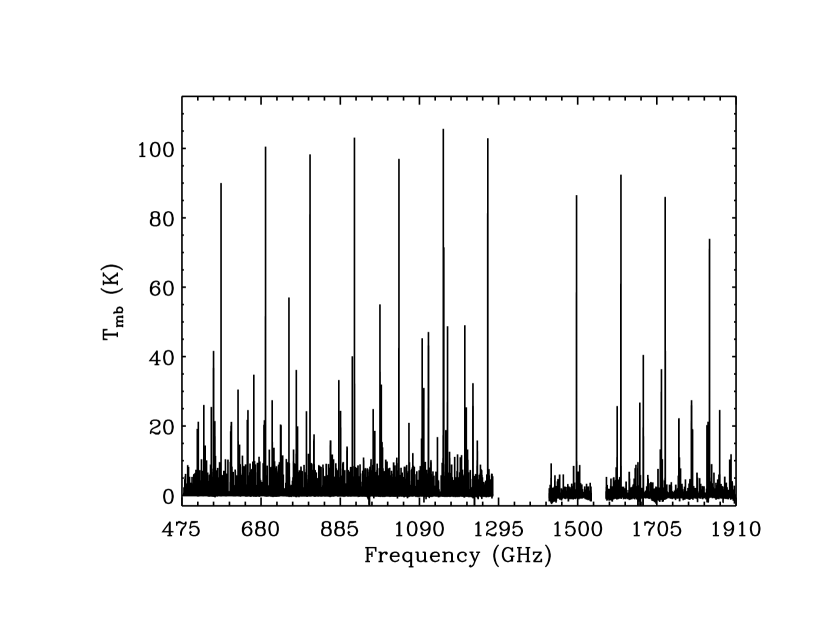
Figure 1: The Orion KL HIFI spectral survey is plotted after baseline subtraction. For bands 6 and 7, the hot core pointing is plotted. The data are resampled uniformly to a velocity resolution of $\sim$ 10 km/s to improve the appearance at this scale.

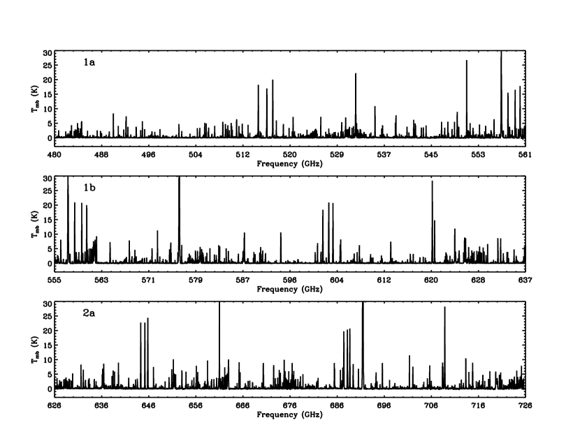
Figure 2: Bands 1a, 1b, and 2a of the HIFI spectral survey toward Orion KL. The data are resampled to a velocity resolution of $\sim$ 10 km/s to improve the appearance at this scale. Each band is labeled in the upper left hand corner of each panel.

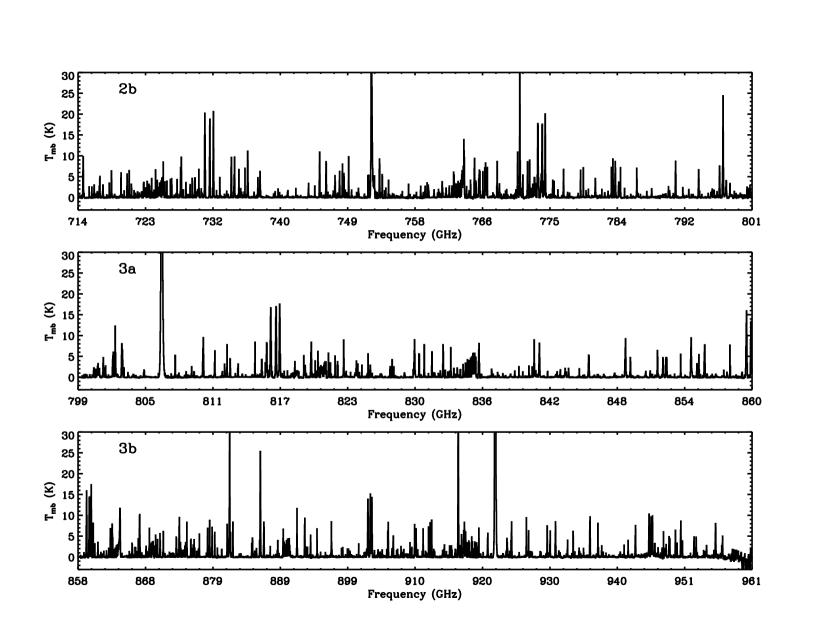
Figure 3: Same as Fig. 2 for bands 2b, 3a, and 3b.

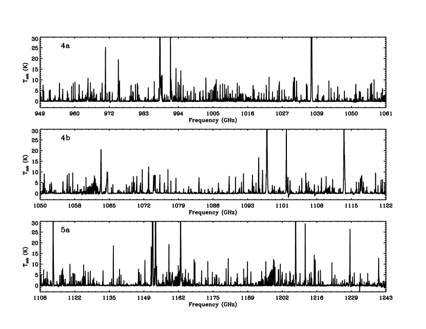
Figure 4: Same as Fig. 2 for bands 4a, 4b, and 5a.

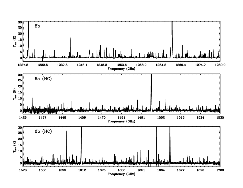
Figure 5: Same as Fig. 2 for bands 5b, 6a, and 6b. The hot core pointing is plotted for band 6.

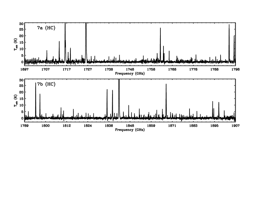
Figure 6: Same as Fig. 2 for bands 7a and 7b. Only the hot core pointing is plotted.

All scans were corrected for aperture efficiency using Eqs. 1 and 2 from Roelfsema et al. (2012). In bands 1 – 5, we applied the aperture efficiency, which is linked to a point source, because the Herschel beam is large relative to the size of the hot core and compact ridge ($\sim$10″). For bands 6 and 7, on the other hand, we applied the main beam efficiency because the beam size is comparable to the size of the hot core and compact ridge and the main beam efficiency is coupled to an extended source. We, however, refer to all line intensities as main beam temperatures, $T_{\rm mb}$, in this work for the sake of simplicity. Fig. 1 plots the entire HIFI spectral survey toward Orion KL. From the figure, the high sub-mm line density, characteristic of Orion KL, is readily apparent. Figs 2 – 6 plot each band individually so that more details of the spectrum can be seen. In particular, these figures show a marked decrease in the observed line density as a function of frequency, which is mainly due to a drop off in the number of emissive transitions from complex organics (Crockett et al., 2010).

In addition to these data products, we also provide SSB spectra with the continuum present. These data were produced by deconvolving DSB spectra after spur removal but before baseline subtraction. The resulting SSB spectra thus contained the continuum but had higher noise levels due to baseline offsets between scans. We next fit a second order polynomial to the continuum in each band. We then added these polynomial fits to the baseline subtracted SSB scans, thus yielding a spectrum which includes the continuum but does not contain the extra noise brought about by baseline offsets. All reduced data products are available online at http://herschel.esac.esa.int/UserProvidedDataProducts.shtml in ASCII, CLASS, and HIPE readable FITS formats. Model fits of individual molecular species (Sec. 3) are also available there.

2.2 The IRAM Survey

In order to constrain the molecular emission at mm wavelengths, we include a spectral survey obtained with the IRAM 30 m telescope in our analysis. This dataset is described in Tercero et al. (2010) and covers frequency ranges 200 – 280 GHz, 130 – 180 GHz, and 80 – 116 GHz, corresponding to spectral windows at 1.3, 2, and 3 mm, respectively, at a spectral resolution of 1.25 MHz corresponding to 1.3 – 4.7 km/s across the IRAM survey. These observations were pointed toward IRc2 at $\alpha_{2000.0}$ = $5^{h}45^{m}14^{s}.5$ and $\delta_{2000}$ = $-5\arcdeg 22\arcmin 30.0\arcsec$. Because the beam size varies between 29″ and 9″, these observations are most strongly coupled to the hot core especially at high frequencies where the beam size is smallest. As a result, our models often over predict emission toward the compact ridge relative to the data in the 1.3 mm band.

2.3 The ALMA Survey

We take advantage of the publicly available ALMA band 6 line survey to investigate the spatial distribution of a subset of molecules detected toward the hot core. This survey was observed as part of ALMA’s science verification (SV) phase and covers a frequency range of 214 – 247 GHz at a spectral resolution of 0.488 MHz ($\sim$ 0.6 km/s at 231 GHz). The observations were obtained with an array of 16 antennas on 20 January 2012. All antennas had a diameter of 12 m and projected baselines had lengths between 13 and 202 k$\lambda$. The phase center was pointed at coordinates $\alpha_{J2000}=5^{h}35^{m}14^{s}.35$ and $\delta_{J2000}=-05^{\circ}22^{\prime}35^{\prime\prime}$. At 231 GHz, ALMA’s primary beam size (field of view) is $\sim$ 27″, similar to Herschel at HIFI frequencies. Callisto and the quasar J0607-085 were used as the absolute flux and phase calibrators, respectively. The Common Astronomy Software Applications package, CASA, was used to produce the maps presented in this work using the same methodology as Neill et al. (2013b). We also employ the publicly available continuum map of Orion KL, derived from 30 line free channels near 230.9 GHz. Both the line survey and continuum map can be downloaded from the ALMA SV website at https://almascience.nrao.edu/alma-data/science-verification.

3 Modeling Methodology

We modeled the emission of each detected molecule, including isotopologues, one at a time. Summing all of the individual fits, thus, yielded the total molecular emission, i.e. the “full band model”. This procedure was carried out by multiple individuals simultaneously, each person modeling several molecules and incorporating the best fit results for other species as determined by other participants, thereby allowing for blended lines to be more quickly identified. The molecular emission was fit using two programs: XCLASS and MADEX (Cernicharo, 2012). We note that two species, CO and H₂O (main isotopologues only), were too optically thick to model with either program as described below. Consequently, we fit Gaussian profiles to these species and include those fits in the full band model.

We use both the HIFI and IRAM surveys to constrain our molecular fits. By combining these datasets, we are essentially modeling the entire spectrum of a given molecule including low energy states, i.e. ground state transitions or close to it, up to energy levels where emission is no longer detected. This is true even for lighter molecules, with widely spaced transitions. Because of the extremely large number of observed lines in the HIFI survey ($\sim$ 13,000; see Sec. 4.1), we do not compile line lists for detected molecules. Rather, we provide a model spectrum for each detected species, from which line intensities for individual transitions can be obtained.

3.1 Description of Orion KL Components

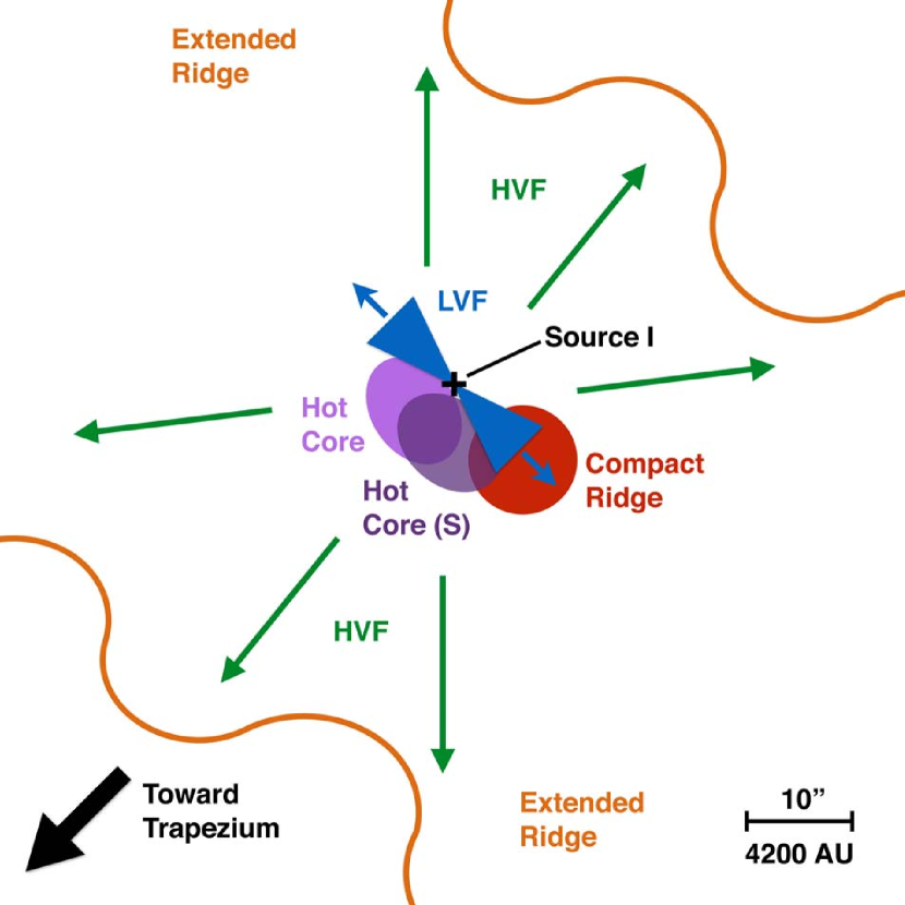
Figure 7: A cartoon illustrating the morphology of Orion KL as seen in the plane of the sky. The spatial/velocity components, which are labelled in the figure, are represented by different colors. The location of radio source I is indicated with a black cross, and the direction of the outflowing gas associated with the LVF and HVF are represented by blue and green arrows, respectively. For orientation, the location of the Trapezium, which lies outside the spatial extent of the cartoon, is indicated with a black arrow. An approximate size scale in arc seconds and AU, assuming a distance of 420 pc, is also given in the lower right hand corner.

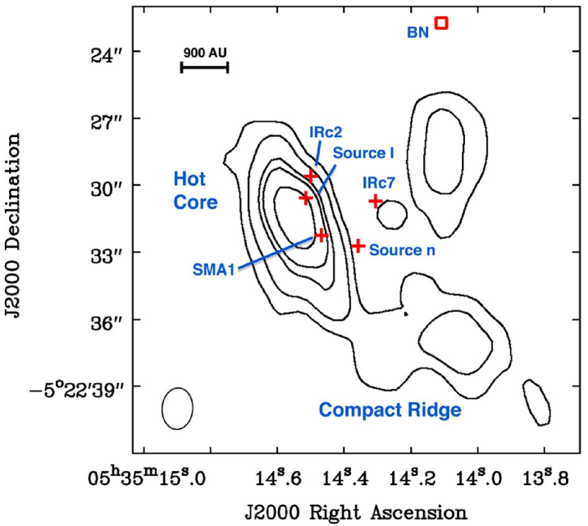
Figure 8: The continuum map of Orion KL at 230.9 GHz taken from the ALMA SV survey. The continuum clumps associated with the hot core and compact ridge are labelled for clarity. Locations of various sources, which are labeled in the plot, are indicated by red crosses (see the text in Sec. 3.1 for details concerning these sources). The position of BN is also represented with a red square. The contour levels correspond to (0.1, 0.2, 0.4, 0.5, 0.75) $\times$ 1.334 Jy beam^-1. A size scale in AU, assuming a distance of 420 pc, is given in the upper left corner and the size of the synthesized beam is indicted by an oval in the lower left corner.

Molecular line emission toward Orion KL originates from several distinct spatial/velocity components. These components are typically labeled as the “hot core”, “compact ridge”, “plateau”, and “extended ridge” (Blake et al., 1987). Using HIFI’s high spectral resolution, we are able to differentiate these components even though they all lie within the Herschel beam because they have line profiles with significantly different velocities relative to the Local Standard of Rest, v_lsr, and full widths at half maximum, $\Delta$v (Blake et al., 1987). A cartoon illustrating the spatial distribution of these components in the plane of the sky is given in Fig. 7 with the different spatial/velocity components labelled. Additionally, we present the ALMA SV continuum map at 230.9 GHz in Fig. 8 which shows more detailed structure toward Orion KL on smaller spatial scales. The continuum clumps associated with the hot core and compact ridge are labelled in Fig. 8 for clarity. We briefly describe each component in the following. When spatial scales (in AU) are reported, we assume an Orion KL distance of 420 pc (Menten et al., 2007; Hirota et al., 2007).

The hot core, so named because it is a hot ($T_{\rm kin}$ $\gtrsim$ 150 K) and dense ($\gtrsim$10⁷ cm^-3) clump of gas which may be harboring one or more massive protostars, is characterized by lines with v_lsr $\approx$ 4 – 6 km/s and $\Delta$v $\approx$ 7–12 km/s. This region, originally detected via inversion lines of ammonia (NH₃; Ho et al., 1979), is in general rich in nitrogen bearing molecules. Interferometric observations of methyl cyanide (CH₃CN) and NH₃ reveal an intricate, clumpy structure on size scales $\lesssim$ 1–2″ ($\lesssim$ 800 AU) and a non-uniform temperature distribution with measured rotation temperatures varying between $\sim$150 – 600 K (Wang et al., 2010; Goddi et al., 2011). The ultimate heating source, however, remains unclear. Both Zapata et al. (2011) and Goddi et al. (2011) conclude that the Orion KL hot core is most likely externally heated, though they disagree on the source, while de Vicente et al. (2002) argues for internal heating by an embedded massive protostar.

The compact ridge is a group of dense clumps of quiescent gas, which are likely externally heated (Wang et al., 2011; Favre et al., 2011), located approximately 12″ ($\sim$ 5000 AU) south-west of the hot core (Figs. 7 and 8). This region is characterized by high densities ($\sim$ 10⁶ cm^-3) and temperatures of $\sim$ 80–150 K (Blake et al., 1987). Line profiles emitted from the compact ridge have narrow line widths, $\Delta$v $\approx$ 3 – 6 km/s and line centers at v_lsr $\approx$ 7 – 9 km/s. Compared to the hot core, the compact ridge is much richer in complex oxygen bearing organics (Blake et al., 1987; Friedel & Snyder, 2008; Beuther et al., 2005).

The plateau, which is characterized by wide line widths ($\Delta$v $\gtrsim$ 20 km/s) at v_lsr $\approx$ 7 – 11 km/s, includes at least two outflows often referred to as the low velocity flow (LVF) and high velocity flow (HVF). The LVF is oriented along a NE – SW axis (Genzel & Stutzki, 1989; Blake et al., 1996; Stolovy et al., 1998; Greenhill et al., 1998; Nissen et al., 2007; Plambeck et al., 2009; Goddi et al., 2009a), and is thought to be driven by radio source I, an embedded massive protostar with no sub-mm or IR counterpart (Menten & Reid, 1995; Plambeck et al., 2009). The HVF, on the other hand, is more spatially extended ($>$ 30″) than the LVF and is oriented along a NW–SE axis, perpendicular to the LVF (Allen & Burton, 1993; Chernin & Wright, 1996; Schultz et al., 1999; O’dell, 2001; Doi et al., 2002; Nissen et al., 2012). Fig. 7 illustrates the relative orientation of these two outflows. The most compact part of the LVF as traced by interferometric observations of SiO (Plambeck et al., 2009) is indicated by a blue hour-glass, though we note the full spatial extent of the LVF is somewhat larger ($\sim$ 30″, see Sec. 3.3). There have been several suggestions as to the ultimate power source behind the HVF. Vibrationally excited transitions of methanol (CH₃OH), cyanoacetylene (HC₃N), and sulfur dioxide (SO₂) have been detected toward the sub-mm source SMA1 (Beuther et al., 2004), possibly indicating the presence of an embedded protostar, which Beuther & Nissen (2008) suggest may be driving the HVF. Plambeck et al. (2009), on the other hand, argue that the HVF is merely a continuation of the LVF. Yet another possibility is that the HVF is powered by the dynamical decay of a multi star system possibly involving radio source I, IR source n, and BN (Rodríguez et al., 2005; Gómez et al., 2005, 2008; Zapata et al., 2009; Bally et al., 2011; Nissen et al., 2012). Both source n and BN are themselves strong IR continuum emitters which likely harbor embedded self-luminous sources (Becklin & Neugebauer, 1967; Lonsdale et al., 1982; Menten & Reid, 1995; Gezari et al., 1998; De Buizer et al., 2012). For orientation, we indicate the positions of radio source I, SMA1, IR source n and BN in Fig. 8. We also indicate the locations of two “infrared clumps”, IRc2 and IRc7, which are adjacent to the hot core (Rieke et al., 1973; Gezari et al., 1998).

The extended ridge represents the most widespread, quiescent gas toward Orion KL ( Fig. 7). Measured rotation temperatures are typically $\lesssim$ 60 K and the line profiles are narrow, $\Delta$v $\approx$ 2 – 4 km/s, with line centers at v_lsr $\approx$ 8 – 10 km/s (Blake et al., 1987). The extended ridge is rich in unsaturated, carbon rich species indicating the dominance of exothermic ion-molecule reactions that do not require activation energies (Herbst & Klemperer, 1973; Watson, 1973; Smith, 1992; Ungerechts et al., 1997).

3.2 Hot Core South

In the course of modeling the data, we noticed that several molecules contained a spectral component with $\Delta$v $\sim$ 5 – 10 km/s and v_lsr $\sim$ 6.5 – 8 km/s, in between line parameters typically associated with the hot core and compact ridge. The presence of this type of component was noted previously by Neill et al. (2013b) who present a detailed analysis of water and HDO emission in the Orion KL HIFI survey. Specifically, HD¹⁸O lines detected in the HIFI scan have an average v_lsr = 6.7 km/s and $\Delta$v = 5.4 km/s, consistent with this “in between” component. Using HDO interferometric maps obtained from the ALMA-SV line survey of Orion KL (Sec. 2.3), the Neill et al. (2013b) study showed that this emission likely originates from a high water column density clump approximately 1″ south of the hot core sub-mm continuum peak.

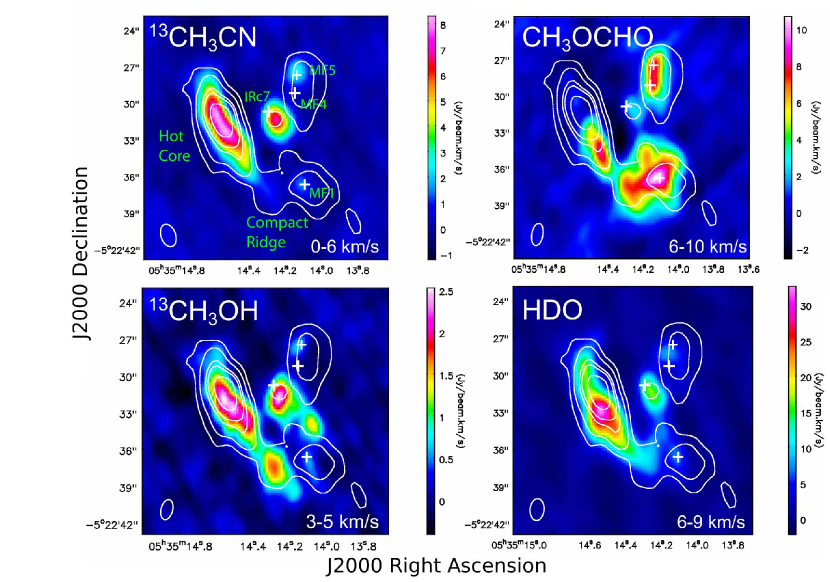
Figure 9: Integrated intensity maps obtained from lines in the ALMA-SV dataset plotted as a color scale. The velocity range over which the intensity is integrated is given in each panel. The transitions plotted are ¹³CH₃CN 13₂ – 12₂ (upper left), ¹³CH₃OH-E 5₂ – 4₂ (lower left), HDO 3_1,2 – 2_2,1 (lower right), and CH₃OCHO 19_6,13 – 18_6,12 (upper right). We only show integrated emission in the range 3 – 5 km/s for ¹³CH₃OH because we wanted to avoid contamination from the compact ridge. The continuum at 230.9 GHz is overlaid in each panel as white contours. The contour levels correspond to (0.1, 0.2, 0.4, 0.5, 0.75) $\times$ 1.334 Jy beam^-1. The synthesized beam size is indicated by an oval in the lower left corner of each panel.

We employ the ALMA-SV dataset here to map, in addition to HDO, ¹³CH₃OH, another species which contains an “in between” component in the HIFI scan (v_lsr = 7.5 km/s, $\Delta$v = 6.5 km/s), ¹³CH₃CN, a hot core tracer with typical line parameters for that region (v_lsr $\approx$ 5.5 km/s, dv $\approx$ 8 km/s), and methyl formate (CH₃OCHO), a prominent compact ridge tracer also with typical line parameters (v_lsr $\approx$ 8 km/s, $\Delta$v $\approx$ 3 km/s). Fig. 9 contains four panels each plotting an integrated intensity map (color scale) of a transition from one of these molecules. The continuum at 230.9 GHz is overlaid as white contours in each panel. White crosses indicate the locations of IRc7, and methyl formate peaks MF1, MF4, and MF5 in the notation of Favre et al. (2011). The sub-mm clump associated with the hot core is also labeled. We used the same data product presented in Neill et al. (2013b) to make Fig. 9.

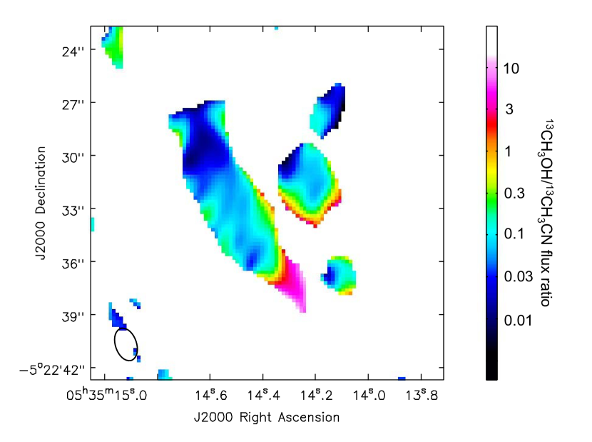
Figure 10: The integrated intensity ratio of the ¹³CH₃OH-E map to ¹³CH₃CN given in Fig. 9 showing the increase in methanol emission relative to methyl cyanide from north to south. The synthesized beam size is indicated by an oval in the lower left corner.

From Fig. 9, we see that ¹³CH₃CN traces the hot core continuum closely while HDO, as first pointed out by Neill et al. (2013b), traces a clump $\sim$ 1″ south of the continuum peak. The ¹³CH₃OH map in Fig. 9 is integrated in the velocity range 3 – 5 km/s to avoid emission from the compact ridge, which methanol also traces. As such, Fig. 9 shows that ¹³CH₃OH emission from the “in between” component does not originate from the compact ridge as traced by methyl formate. Rather, this emission is strongest just south of where ¹³CH₃CN peaks. Because the difference is more subtle than with HDO, Fig. 10 plots the ¹³CH₃OH/¹³CH₃CN integrated intensity ratio, which shows a clear gradient in ¹³CH₃OH emission relative to ¹³CH₃CN from north to south. Given that HDO and ¹³CH₃OH both trace regions south of the ¹³CH₃CN peak, we assume other molecules displaying emission from this “in between” component originate from a similar region. We thus label this component “hot core south” or hot core (s), which we represent schematically in the cartoon presented in Fig. 7.

3.3 XCLASS modeling

All molecular species are modeled using XCLASS. This program uses both the CDMS (Müller et al., 2001, 2005, http://www.cdms.de) and JPL (Pickett et al., 1998, http://spec.jpl.nasa.gov) databases to produce model spectra assuming local thermodynamic equilibrium (LTE). Input parameters are the telescope diameter, $D_{\rm tel}$, source size, $\theta_{s}$, rotation temperature, $T_{\rm rot}$, total column density, $N_{\rm tot}$, line velocity relative to the Local Standard of Rest, v_lsr, and line full width at half maximum, $\Delta$v. In order to account for dust extinction, the dust optical depth, $\tau_{d}$, is parameterized by a power law,

$$\tau_{d}=2m_{H}(\chi_{\rm dust})N_{H_{2}}\kappa_{1.3\rm mm}\left(\frac{\nu}{230\ GHz}\right)^{\beta},$$ (1)

where $N_{\rm H_{2}}$ is the H₂ column density, $\kappa_{1.3\rm mm}$ is the dust opacity at 1.3mm (230 GHz), $\beta$ is the spectral index, $m_{\rm H}$ is the mass of a hydrogen atom, and $\chi_{\rm dust}$ is dust to gas mass ratio. As outlined below, we hold $N_{\rm H_{2}}$ and $\theta_{s}$ fixed for a given spatial/velocity component, but note that there are several exceptions in which we varied $\theta_{s}$ to obtain better agreement between the models and data. These instances are explained in Sec. 5. We also set $D_{\rm tel}$ = 3.5 m and 30 m when comparing our models to the HIFI and IRAM surveys, respectively. We varied $T_{\rm rot}$, $N_{\rm tot}$, v_lsr, and $\Delta$v as free parameters. Additional information regarding XCLASS, e.g. specific equations used in the code, can be found in Comito et al. (2005) and Zernickel et al. (2012).

We assume that all molecules emitting from the same spatial/velocity component have the same source size, which is a simplifying assumption. The aim of this study, however, is not a detailed analysis of any single molecule. It is a holistic analysis of the entire spectrum. This is therefore a reasonable approximation and is in line with previous spectral survey papers of Orion KL (see e.g. Tercero et al., 2010, 2011). Adopted source sizes for each spatial/velocity component are given in Table 2. We estimate $\theta_{s}$ for the hot core and compact ridge using interferometric observations from Beuther & Nissen (2008) and Favre et al. (2011), respectively. The plateau source size was obtained from Herschel/HIFI water maps taken as part of the HEXOS program (Melnick et al. 2014, in preparation). Finally, we assume a source size of 180″ for the extended ridge to reflect the fact that the extended ridge completely fills the Herschel beam at all frequencies. For several molecules, we were forced to use $\theta_{s}$ values that differed from those given in Table 2. These deviations are explained in the descriptions of individual molecular fits presented in Sec. 5. Estimates of $N_{\rm H_{2}}$ for each spatial/velocity component are also given in Table 2. We obtained these values from Plume et al. (2012), who use C¹⁸O lines within the Orion KL HIFI scan to derive total C¹⁸O column densities which they convert to $N_{\rm H_{2}}$ estimates by assuming a CO abundance of 1.0 $\times$ 10^-4 and ¹⁶O / ¹⁸O = 500. We modified the H₂ column densities for the compact ridge and plateau because the Plume study assumed source sizes for these components that are different from what we adopt here. Consequently, we recalculated the C¹⁸O upper state columns assuming the source sizes used in this study and applied the same correction factors reported by Plume et al. (2012).

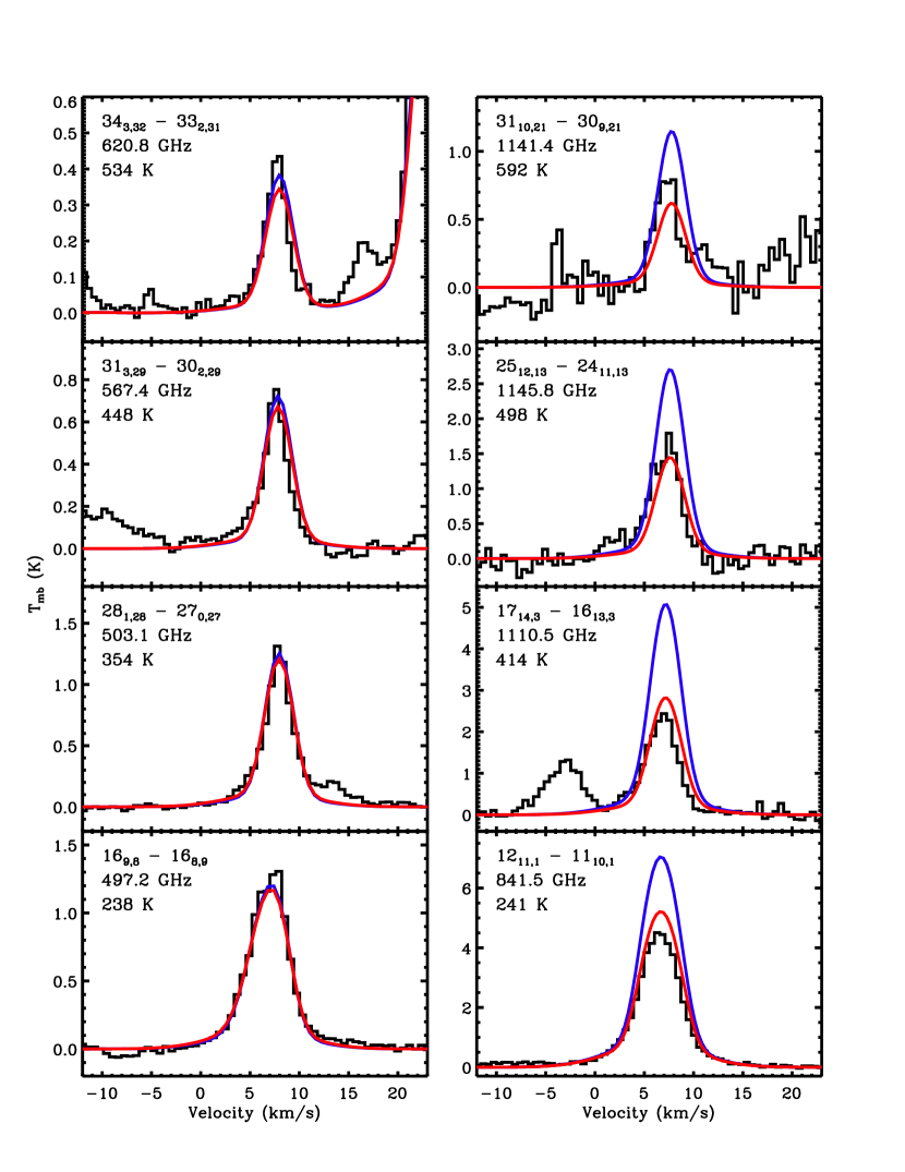
Figure 11: A sample of 8 CH₃OCH₃ lines from the HIFI scan. The data are plotted in black and the quantum numbers, rest frequency, and $E_{\rm up}$ for each transition are labeled from top to bottom in each panel. We use the quantum numbers from the EA spin isomer, but note that transitions from AA, EE, AE, and EA-CH₃OCH₃ are blended together at HIFI frequencies. The red and blue lines represent XCLASS models which assume $N_{\rm H_{2}}$ = 2.5 $\times$ 10²⁴ cm^-2 and 3.9 $\times$ 10²³ cm^-2 and set $N_{\rm tot}$ = 6.5 $\times$ 10¹⁶ cm^-2 and 5.9 $\times$ 10¹⁶ cm^-2, respectively. Both models set $T_{\rm rot}$ = 110 K and $\theta_{s}$ = 10″. Dimethyl ether is also detected toward the hot core, but this component is not emissive for the transitions plotted here.

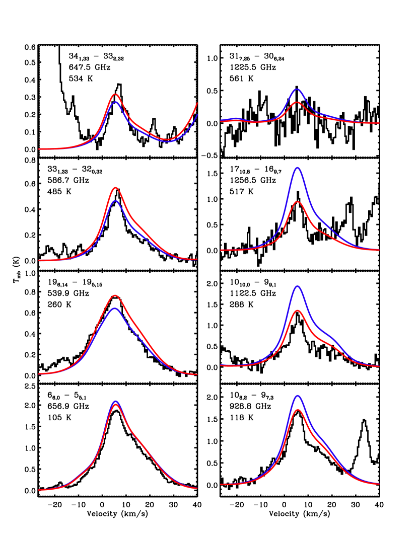
Figure 12: A sample of 8 ³⁴SO₂ lines from the HIFI scan. The data are plotted in black and the quantum numbers, rest frequency, and $E_{\rm up}$ for each transition are labeled from top to bottom in each panel. The red and blue lines represent XCLASS models which assume $N_{\rm H_{2}}$ = 2.5 $\times$ 10²⁴ cm^-2 and 3.9 $\times$ 10²³ cm^-2, respectively. Each model has a hot core and plateau component. The model plotted in red sets $N_{\rm tot}$ = 5.0 $\times$ 10¹⁵ and 4.7 $\times$ 10¹⁵ cm^-2, while the model plotted in blue sets $N_{\rm tot}$ = 3.5 $\times$ 10¹⁵ and 3.0 $\times$ 10¹⁵ cm^-2 for the hot core and plateau components, respectively. Both models set $T_{\rm rot}$ = 240 K and 150 K and $\theta_{s}$ = 10″and 30″ for the hot core and plateau components, respectively. There are additional cooler sub-components present in these models to fit the emission at lower excitation for both the hot core and plateau. These sub-components, however, are not significantly emissive for the plotted transitions.

For the dust extinction power law, we assume $\kappa_{1.3\rm mm}$ = 0.42 cm² g^-1, corresponding to the midpoint between bare grains and grains with thin ice mantles (Ossenkopf & Henning, 1994). We also set $\beta$ = 2 and $\chi_{\rm dust}$ = 0.01. In the course of modeling the data, we found that the $N_{\rm H_{2}}$ values given Table 2 tended to underestimate the extinction necessary to reproduce the emission in the highest frequency bands where the dust optical depth is highest. In other words, molecules fit well at frequencies below $\sim$ 1 THz always tended to be over predicted at higher frequencies. As a result, we use a higher $N_{\rm H_{2}}$ estimate to compute the dust optical depth. We adopt a value of $N_{\rm H_{2}}$ = 2.5 $\times$ 10²⁴ cm^-2 for the hot core, compact ridge, and plateau. Because the extended ridge represents lower density gas that is not as heavily embedded, we retain the $N_{\rm H_{2}}$ value given in Table 2 for this spatial/velocity component. Fig. 11 plots 8 transitions of dimethyl ether (CH₃OCH₃), a prominent compact ridge tracer. The panels are organized so that both columns span a range in upper state energy, $E_{\rm up}$, from $\sim$ 200 to 600 K with $E_{\rm up}$ increasing from bottom to top. Lines in the left and right columns occur at frequencies below and above 800 GHz, respectively. Transitions in the left column are therefore less affected by dust extinction than the right with both columns covering similar ranges in $E_{\rm up}$. The red line corresponds to an XCLASS fit which sets $N_{\rm H_{2}}$ = 2.5 $\times$ 10²⁴ cm^-2, while the blue line represents a similar model that assumes the H₂ column density given in Table 2. Dimethyl ether column densities for the higher and lower extinction fits are 6.5 $\times$ 10¹⁶ cm^-2 and 5.9 $\times$ 10¹⁶ cm^-2, respectively. Both models set $T_{\rm rot}$ = 110 K and $\theta_{s}$ = 10″. From the plot, we see that the model with greater dust extinction fits the data better than the lower extinction model over all frequencies. Because similar ranges in $E_{\rm up}$ are covered at low and high frequencies, it is not possible to improve the fit at lower extinction by changing either $T_{\rm rot}$ or $\theta_{s}$. We observed the same trend for molecules detected toward the hot core and plateau. Fig. 12 plots a sample of 8 transitions of ³⁴SO₂, a molecule with strong hot core and plateau components, organized in the same way as Fig. 11, with red and blue lines representing an analogous set of XCLASS models. We again see better agreement for the higher extinction model. The $N_{\rm H_{2}}$ we adopt to compute $\tau_{d}$ is between 6 and 9 times larger than the H₂ column densities derived toward the hot core, compact ridge, and plateau using C¹⁸O line emission, but is commensurate with other $N_{\rm H_{2}}$ estimates derived from mm and sub-mm observations which report $N_{\rm H_{2}}$ $\gtrsim$ 10²⁴ cm^-2 (Favre et al., 2011; Mundy et al., 1986; Genzel & Stutzki, 1989). This difference could be resolved by assuming a higher dust opacity, i.e. increasing $\kappa_{1.3\rm mm}$ by the same factor $N_{\rm H_{2}}$ is reduced (see Eq. 1). However, because this adjustment would result in the same $\tau_{d}$, we use the higher $N_{\rm H_{2}}$ and conclude a dust optical depth which obeys the relation,

$$\tau_{d}=3.5\times 10^{-2}\left(\frac{\nu}{230\ GHz}\right)^{2}$$ (2)

produces the required dust extinction to accurately fit the data across the entire HIFI band.

We fit an XCLASS model to the emission of each molecule by first selecting a sample of transitions with varying line strengths that covered the entire range in excitation energy over which emission was detected. For simple species, with relatively few lines, this was straightforward. For more complex organics, however, we had many lines, thousands in some cases, from which to choose. Care was taken to select lines that were not blended with any other species. This was done by overlaying the full band model and observed spectrum while we selected transitions on which to base our fit. Because the full band model is the sum of all molecular fits, it evolved as the individual molecular fits changed. Once a sample of lines was selected, each transition was plotted simultaneously in a different panel with the panels arranged so that the upper state energy increased from the lower left panel to the upper right. The emission was then fit by varying the free parameters (i.e. $T_{\rm rot}$, $N_{\rm tot}$, v_lsr, and $\Delta$v) by hand until good agreement, as assessed by eye, was achieved between the data and models at all excitation energies. At this point, we computed a reduced $\chi^{2}$ metric (described in the Appendix) for each model across the entire HIFI band in order to determine how well the models reproduced the data relative to one another, and to identify those fits which could be improved. Model fits were then revised iteratively.

We found that automated fitting algorithms had difficulty reaching reasonable solutions, especially when multiple spatial/velocity components and/or temperature gradients were required. Weaker species ($T_{\rm peak}$ $\lesssim$ 1 K) that had observed line intensities close to the noise, combined with the prevalence of line blends presented additional difficulties in assessing the goodness of fit with these algorithms. As a result, we derived most models by hand. However, in some instances, when a sample of strong unblended transitions was available, we employed the MAGIX program (Möller et al., 2013), which optimizes the output of other numerical codes (XCLASS in this case), to automate the fitting process using a Levenberg-Marquardt algorithm. MAGIX utilizes a subset of observed transitions supplied by the user to assess the goodness of fit for a given molecule. Consequently, we carried out by hand alterations to these fits once reduced $\chi^{2}$ calculations were performed over the entire HIFI band as described above.

When we observed more than one isotopologue for a given molecule, effort was made to produce models which used consistent values for $T_{\rm rot}$, $\Delta$v, and v_lsr for all isotopic species. We, however, sometimes made small adjustments to these parameters to get the optimum fit. The major difference between the models is thus the column density, the ratio of which should be equal to the isotopic abundance ratio. Among rarer isotopologues, isotopic ratios inferred from our models are commensurate with those derived previously toward Orion KL (Tercero et al., 2010; Blake et al., 1987) indicating optically thin emission. Our models, however, also indicate that many of the most abundant isotopologues are optically thick, meaning our models likely underestimate $N_{\rm tot}$. Furthermore, we often had to fit very optically thick isotopologues with higher rotation temperatures than their more optically thin counterparts in order to reproduce the observed line intensities over all energies. Emission from these species therefore is too optically thick from which to derive reliable $T_{\rm rot}$ and $N_{\rm tot}$ values using XCLASS. As a result, these models serve mainly as templates for the molecular emission. Species that fall into this category are marked with an “X” in Table 3. This table is broken down by spatial/velocity component because a particular molecule may not be optically thick in all of its components.

While modeling the hot core and plateau with XCLASS, we found that, for some molecules, a single temperature fit failed to reproduce the observed emission, which suggests the presence of temperature gradients in these components. This was most apparent when trying to simultaneously fit both the IRAM and HIFI data. Because the IRAM data, in general, probed lower energy transitions compared to HIFI, the IRAM spectra sometimes required additional cooler sub-components in order for a single model to fit both datasets well. We, therefore, included additional sub-components when necessary to simulate temperature gradients. For the hot core, the sub-component responsible for most of the emission in the HIFI scan always had a source size of 10″. Hotter or cooler sub-components were then added such that the source size increased or decreased by successive factors of two. Temperature gradients were organized such that $T_{\rm rot}$ increased as $\theta_{s}$ decreased (i.e. the more compact emission is hotter), corresponding to an internally heated clump. We chose this convention based on more detailed non-LTE models presented by Neill et al. (2013b) and Crockett et al. (2014) which fit the H2O/HDO and H2S emission, respectively, within the HIFI scan. In order to reproduce the observed emission of these species, their models require enhanced near and far-IR radiation fields relative to what is observed, suggesting the presence of a self-luminous source or sources within the hot core. Moreover, ethyl cyanide (C₂H₅CN) transitions observed within the ALMA SV survey show that more highly excited C₂H₅CN lines originate from a more compact region than lower lying transitions (Favre et al. 2014, in preparation). For the plateau, we kept a 30″ source size for all sub-components to simulate the fact that the plateau fills most of the Herschel beam at HIFI frequencies. We did not need temperature gradients to fit the compact ridge or extended ridge in our XCLASS models.

Our final XCLASS models are plotted in Figure Set 13 available in the online edition. In this set, each molecule is represented by a figure in which a sample of transitions is plotted covering the entire range in excitation energy over which that species is detected. At least one transition is plotted in each panel, and the panels are organized so that $E_{\rm up}$ increases from the lower left panel to the upper right. The lowest energy panels often show transitions observed in the IRAM scan. The quantum numbers corresponding to the transition at the center of each panel are labeled. The solid blue line represents the XCLASS model for the molecule being considered, the solid green line corresponds to the model emission from all other molecules, and the dashed red line is the model for all detected species (the sum of the former two curves). Figs. 13.13, 13.33, and 13.66 show examples from Figure Set 13, which plot the molecular fits for H¹³CN, a polyatomic linear rotor, H₂CS, an asymmetric rotor, and CH₃OCHO, a complex organic, respectively. These figures illustrate the diversity in observed line profiles not only between molecules which trace different spatial/velocity components but also from the same species at different excitation energies. The latter arises because the hot core, compact ridge, plateau, and extended ridge are emissive over different ranges in excitation energy.

XCLASS model parameters for molecular fits from which we obtain robust $T_{\rm rot}$ and $N_{\rm tot}$ information are given in Table 4. We do not include models marked in Table 3 because they do not provide any physical information. We estimate the uncertainty in our derived $T_{\rm rot}$ and $N_{\rm tot}$ values to be approximately 10% and 25%, respectively. Our estimated error in v_lsr is $\pm$ 1 km/s for the hot core, compact ridge, and extended ridge, and $\pm$ 2 km/s for the plateau. We also estimate $\Delta$v errors of $\pm$ 0.5 km/s, 1.5 km/s, and 5.0 km/s, for the compact/extended ridge, hot core, and plateau, respectively. These uncertainty calculations are described in the Appendix.

3.4 MADEX modeling

A subset of the molecules detected in the HIFI scan were also modeled using the MADEX code. When collisional excitation rates are available, this non-LTE program solves the equations of statistical equilibrium assuming the large velocity gradient (LVG) approximation based on the the formalism of Goldreich & Kwan (1974). MADEX computes transition frequencies and line strengths for most molecules directly from an internal database of rotation constants and dipole moments. For a small fraction ($\sim$6%) of molecules, however, frequencies and line strengths are taken directly from the JPL and CDMS catalogs. If collision rates do not exist for a given molecular species, model spectra can also be computed assuming LTE. Just as with XCLASS, model input parameters include: $D_{\rm tel}$, $\theta_{s}$, $N_{\rm tot}$, v_lsr, and $\Delta$v. Because MADEX is a non-LTE code, the user must also set the kinetic temperature, $T_{\rm kin}$, and the H₂ volume density, $n_{\rm H_{2}}$. We take $\theta_{s}$, $T_{\rm kin}$, $n_{\rm H_{2}}$, $N_{\rm tot}$, v_lsr, and $\Delta$v to be free parameters. However, as described in more detail below, we attempt to use consistent $T_{\rm kin}$ and $n_{\rm H_{2}}$ values for a given spatial/velocity component, especially when modeling a gradient, and apply $\theta_{s}$ values that are similar to those used with XCLASS. We also set $D_{\rm tel}$ = 3.5 m and 30 m when modeling the HIFI and IRAM surveys, respectively, consistent with XCLASS. Additionally, the user can also specify a spatial offset from the center pointing position, $\Delta\theta$, to account for differences in the telescope response. For the hot core and compact ridge we adopt a $\Delta\theta$ value of 3″ and do not apply any spatial offsets for the plateau or extended ridge. These values were obtained from a 2D line survey of Orion KL taken with the IRAM 30 m telescope (Marcelino et al. 2014, in preparation).

Our modeling approach is similar to previous studies which use MADEX to model molecular emission within the IRAM survey (Marcelino et al. 2014, in preparation; Tercero et al., 2010, 2011; Esplugues et al., 2013a, b). The molecules we model using MADEX are: CH₃CN, HCN, HNC, HCO⁺, SO, SO₂, and their isotopologues. These molecules are chosen because they have existing collision rates for states probed by HIFI. This group also includes a complex organic as well as simpler 2 and 3 atom molecules. In addition, these species are detected toward almost every spatial/velocity component. (We do not detect CH₃CN and SO toward the extended ridge and compact ridge, respectively). Temperature and density gradients surely exist within these components (see e.g. Wang et al., 2011, 2010). As a result, we model all but the extended ridge and, in some cases, the compact ridge with multiple sub-components which vary both $T_{\rm kin}$ and $n_{\rm H_{2}}$ to simulate such gradients. Utilizing MADEX in this way, thus, allows us to compare the column densities, and ultimately molecular abundances, derived from our XCLASS LTE models to more advanced non-LTE calculations, which include both temperature and density gradients. In particular, we are able to determine if including density gradients significantly affects the determination of molecular abundances toward the different spatial velocity/components. Where possible, we have used the same values for $\Delta$v, v_lsr, $\theta_{s}$, $T_{\rm kin}$, and $n_{\rm H_{2}}$ for the sub-components, allowing only the column density to vary. In order to obtain better agreement between the data and model, however, slight adjustments were needed in some cases. The need for these adjustments likely indicates the sensitivity of these molecules to the complex underlying physical structure of Orion KL. Just as with XCLASS, these parameters were varied by hand.

Temperature and density gradients are organized in the following way. For the hot core, sub-components have source sizes between 10″ and 5″ with $n_{\rm H_{2}}$ and $T_{\rm kin}$ decreasing with increasing source size, thus simulating an internally heated cloud which is densest closest to the central heating source. For the compact ridge, sub-component source sizes vary between 10″ and 20″ with temperature and density gradients organized such that $n_{\rm H_{2}}$ decreases and $T_{\rm kin}$ increases with increasing source size. This setup corresponds to an externally heated dense clump, roughly approximating the structure of the compact ridge (Wang et al., 2011; Favre et al., 2011). Sub-components for the plateau have source sizes in the range 10″ – 30″ with temperature and density gradients organized in the same way as the hot core. The assumption here being that the denser parts of the outflow subtend a smaller area in the Herschel beam. We note that the same source size is used when fitting a temperature gradient to SO and SO₂ in the plateau, which are both fit with lower (v_lsr = 6.0 km/s) and higher (v_lsr = 11.0 km/s) velocity components. Source sizes used in the MADEX models are therefore commensurate with those used in the XCLASS fits.

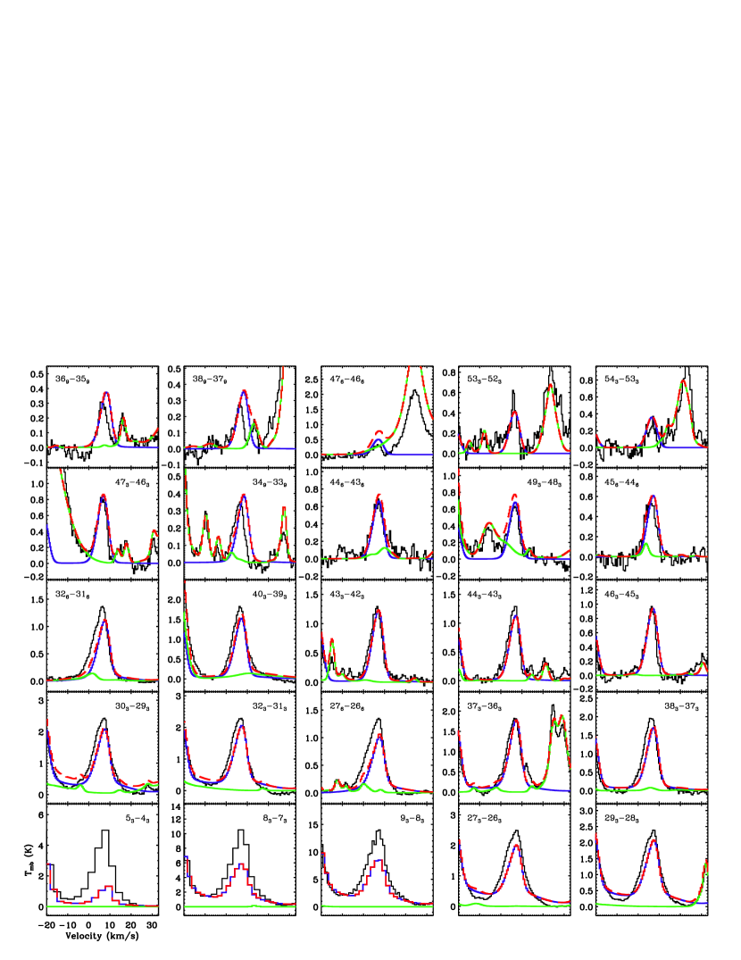
Figure 14.1: Observed transitions in the HIFI and IRAM surveys (black) with the MADEX model for CH₃CN-A overlaid as a blue solid line. Modeled emission from all other species (solid green) along with the total fit (dashed red) are also overlaid. Quantum numbers labeling each transition are given in each panel and excitation energy increases from the lower left panel to the upper right. See Sec. 5 for a description of the quantum numbers.

Our MADEX models are plotted in Figure Set 14 available in the online edition. In this set, we follow the same conventions as Figure Set 13, plotting the same sample of transitions for the MADEX and XCLASS fits. Figs. 14.1 and 14.14 show samples from Figure Set 14, which plot our models for CH₃CN-A, a complex organic, and ³⁴SO, a linear rotor with electronic angular momentum, respectively. Model parameters for those species fit with MADEX are given in Table 5. Just as in Table 4, we only list model parameters for the optically thin isotopologues from which reliable column densities can be derived. We estimate the uncertainty in our derived column densities to be approximately 25%, and adopt the same errors for v_lsr and $\Delta$v as our XCLASS models. The uncertainty in these values are described in more detail in the Appendix. Although $T_{\rm kin}$ and $n_{\rm H_{2}}$ are, in principle, free parameters in our MADEX models, we do not report uncertainties for these quantities because, during the modeling process, these values were, for the most part, held fixed for a given spatial/velocity component. That is, we a priori assumed the temperature/density structure of a spatial/velocity component, (via one or more temperature/density sub-components), and only changed these parameters when varying $N_{\rm tot}$ did not significantly improve the fit.

4 Results

4.1 The Full Band Model and Line Statistics

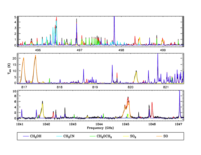
Figure 15: Three selected spectral regions from the HIFI survey. The data are plotted in black and the full band model is overlaid in red. Other colors correspond to individual molecular fits which are labeled in a legend at the bottom of the plot. The overlaid individual fits include emission from all detected isotopologues and vibrationally excited states.

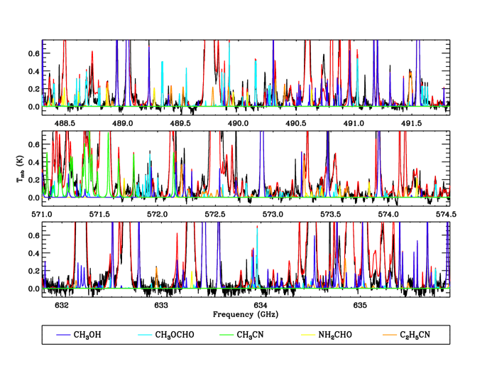
Figure 16: Three selected spectral regions from the HIFI survey which highlight weak emission ($T_{\rm mb}$ $<$ 1 K) originating principally from complex organics. The same conventions as Fig. 15 are followed here.

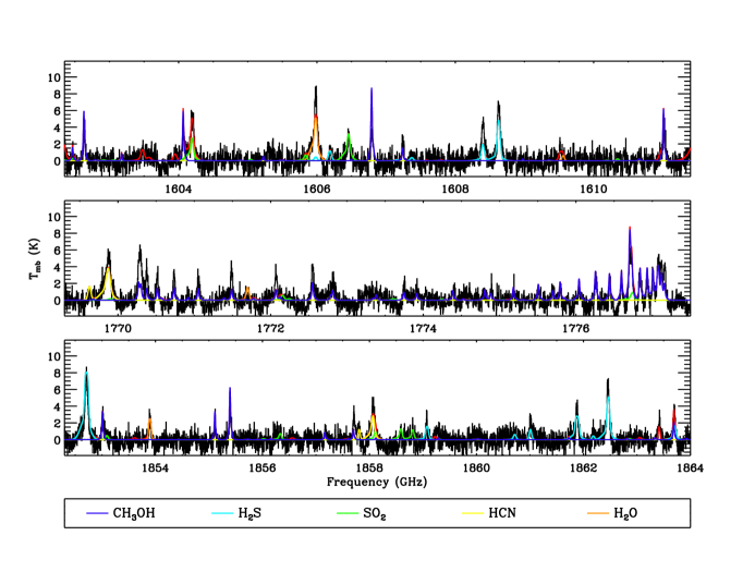
Figure 17: Three selected spectral regions from the HIFI survey displaying emission from band 6 and 7, the highest frequency bands in the HIFI survey. The same conventions as Fig. 15 are followed here.

In total, we detect 79 isotopologues of 39 molecules. Emission from each species has been modeled simultaneously over the entire bandwidths of the HIFI and IRAM surveys. We, in general, find excellent agreement between the data and models. Summing the molecular fits, we obtain the full band model for Orion KL. Fig. 15 plots three sections from the HIFI spectrum with the full band model overlaid as a solid red line. Individual models for the five most emissive molecules in these regions are also overlaid as different colors. Fig. 15 focuses on frequencies less than 1280 GHz and intensity scales $\geq$ 5 K. The plot thus gives a flavor for how well the full band model reproduces strong lines in bands 1a – 5b. Fig. 16, on the other hand, plots three regions at the low frequency end of the survey at $T_{\rm mb}$ levels less than 0.8 K, highlighting weak emission fit by the full band model largely from complex organics. A similar sample of three spectral regions in bands 6 and 7, the highest frequency bands in the HIFI survey, is plotted in Fig. 17. We see from this plot that the high frequency bands are dominated by emission from lighter species, the exception being CH₃OH, which is the only complex organic detected at these frequencies.

In order to quantify how well each molecular fit reproduces the data, we compute a reduced chi squared, $\chi_{\rm red}^{2}$, statistic for each model. The $\chi_{\rm red}^{2}$ calculations are described in the Appendix and reported in Table 6 in ascending order along with the database from which we obtained each spectroscopic catalog. Because we are mainly focused on the analysis of the HIFI spectrum in this study, the $\chi_{\rm red}^{2}$ statistic is computed only at HIFI frequencies. Our models make a number of simplifying assumptions. First, the molecular fits approximate temperature, and in the case of MADEX, density gradients in a simple way (i.e. adding multiple sub-components). Second, the XCLASS models assume LTE level populations. Third, both XCLASS and MADEX do not include radiative excitation effects which are likely important for some species, especially those with detected vibrational modes. And fourth, we assume the emitting source size does not change as a function of excitation energy, though we tried to mitigate this issue by changing the source size toward certain spatial/velocity components when temperature gradients are invoked. As a result, we do not expect all of our fits to have $\chi_{\rm red}^{2}$ $\sim$ 1. These calculations, however, do convey which models reproduce the data best. From Table 6, we see a range of $\chi_{\rm red}^{2}$ values from 83 XCLASS models. The number of models is larger than 79, the number detected isotopologues, because, in some instances we fit vibrationally excited emission (see Sec. 4.3) or different spin isomers with separate XCLASS models. We note that 3 XCLASS fits, which model weak or heavily blended emission (¹³C¹⁸O, OD, and HN¹³C), do not have enough usable channels to compute reliable $\chi_{\rm red}^{2}$ values. Table 6 shows that over half, 47 out of 80, of the XCLASS models have $\chi_{\rm red}^{2}$ $\leq$ 1.5 indicating excellent agreement between the data and models. Another group of 18 have $\chi_{\rm red}^{2}$ = 1.6 – 3.0, which by eye fit quite well, but do not agree with the data as closely as those models with $\chi_{\rm red}^{2}$ $\leq$ 1.5. Finally, 15 models have $\chi_{\rm red}^{2}$ $>$ 3.0, which do not reproduce the data as well as the former two categories.

There are several factors that contribute to high $\chi_{\rm red}^{2}$ values in some of our XCLASS models. First, we are unable to get excellent fits for some molecules partially because they are extremely optically thick. Species that fall into this category are: o-NH₃, H₂CO, SO₂, H₂S, CH₃OH-A, and CH₃OH-E. Second, radiative pumping likely plays a significant role in the excitation of several molecules with high $\chi_{\rm red}^{2}$ values producing deviations from our LTE models. H₂O, CH₃OH, H₂S, NH₃, and NH₂, most of which have detected vibrationally/torsionally excited lines in the HIFI band, may, along with their isotopologues, represent such species. We also include in this category the CH₃CN,$\nu_{8}=1$ model which has a $\chi_{\rm red}^{2}$ = 4.0, but note that the ground vibrational mode models fit the data well. In addition to pumping, some of these molecules may not be in LTE possibly indicating they are tracing lower density gas. As a result, our LTE models may be ill suited to reproduce the observed emission. Finally, emission from OH, NH₃, and HCl contain absorption components which we do not fit in this study (see Sec. 5), thus increasing our calculated $\chi_{\rm red}^{2}$ values for these molecules. Table 6 also reports $\chi_{\rm red}^{2}$ statistics for the MADEX models, most of which have values commensurate with their XCLASS counterparts, though they tend to be higher compared to XCLASS. This is, in part, a result of how we performed the MADEX modeling, which was less ad hoc than our XCLASS approach. That is, using MADEX, we took a set of sub-components with given $T_{\rm kin}$ and $N_{\rm H_{2}}$ and adjusted only the column densities to get the best fit, altering the kinetic temperatures and H₂ densities only when $N_{\rm tot}$ adjustments didn’t produce enough improvement in the fit. An additional reason for the higher MADEX $\chi_{\rm red}^{2}$ values, especially for SO₂ and its isotopologues, which have particularly discrepant $\chi_{\rm red}^{2}$ values, is that the MADEX models do not include reddening. Consequently, the largest deviations between the data and fits occur at high frequencies ($\nu$ $\gtrsim$ 1 THz) where SO₂ emission is still strong and the models tends to over predict the observations.

Using our XCLASS models as a template for the data, we compute, for each molecular species, the number of detected lines, $N_{\rm L}$, and total integrated intensity, $\int{T_{mb}}d\rm v$, within the HIFI survey. Integrated intensities are computed separately for each spatial/velocity component and are reported in Table 7 with molecules organized such that the total integrated intensity from all components (last column) is in descending order. For these calculations, we consider a “line” to be any feature with a discernible peak given the resolution of HIFI. Hence, a detected ”line” which contains multiple unresolved hyperfine transitions, for example, is only counted once. In order for a line to be considered detected, it had to have a peak intensity $\geq$ 3 times the local RMS, where we used a single RMS for each band. From Table 7, we see that CH₃OH (sum of A and E) is the most emissive molecule, both in terms of total integrated intensity and number of detected lines. After methanol, the total integrated intensity is dominated by molecules with strong plateau components (e.g. CO, SO₂, and H₂O). Dimethyl ether is the second most emissive complex organic in terms of total integrated intensity, while methyl formate has the highest number of detected lines after methanol and its isotopologues. Summing $N_{\rm L}$ from all modeled species we obtain a total of $\sim$ 13,000 identified lines in the Orion KL HIFI survey at or above 3 $\sigma$.

4.2 Abundances

We compute molecular abundances by dividing the column densities in Tables 4 and 5 by $N_{\rm H_{2}}$ values given in Table 2. We emphasize each complex organic is typically constrained by over 400 lines that, when combined with the mm data, encompasses an extremely broad range of excitation energies. The emission from lighter molecules (e.g. HCN, CS, etc.), with more widely spaced transitions, is also globally constrained in terms of $E_{\rm up}$ because of the wide bandwidth. For the rare isotopologue models, we obtained molecular abundances by multiplying $N_{\rm tot}$ by an assumed isotopic ratio. When more than one isotopologue is observed for a given molecule, they are averaged together. The same isotopologues are used to compute abundances from the XCLASS and MADEX models. That is, we do not use compact or extended ridge components which are invoked in some MADEX models but are not included in corresponding XCLASS fits (see Secs. 5.5, 5.6, 5.15, and 5.16). We assume the following isotopic ratios: ¹²C/¹³C = 45, ³²S/³³S = 75, ³²S/³⁴S = 20, ¹⁶O/¹⁸O = 250, ¹⁴N/¹⁵N = 234, and ³⁵Cl/³⁷Cl = 3. The C, S, and O ratios are taken from Tercero et al. (2010), who derive these values by modeling OCS and H₂CS emission present in the IRAM 30 m line survey using MADEX. The N isotopic ratio is taken from Adande & Ziurys (2012), who compute this value by analyzing CN hyperfine transitions, from which reliable optical depths can be measured. We assume a solar isotopic ratio for Cl (Asplund et al., 2009).

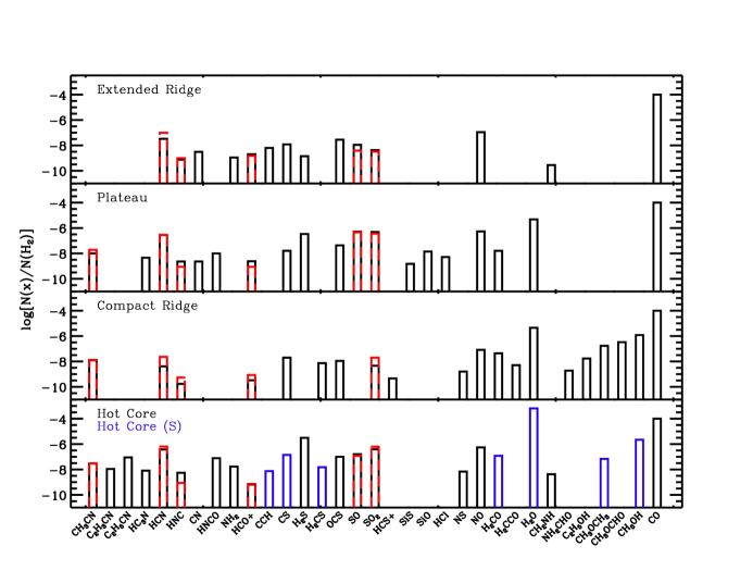
Figure 18: Derived abundances plotted as a function of molecule. Each panel corresponds to a different spatial/velocity component which is labeled in the upper left hand corner of each panel. Abundances derived using XCLASS and MADEX are plotted as solid black and dashed red lines, respectively. XCLASS abundances plotted in blue indicate an origin from hot core (s).

Molecular abundances, derived from our XCLASS models, are given in Table 8. For models with temperature gradients, we add the column densities from the individual sub-components together and take this sum as $N_{\rm tot}$ in our abundance calculations. Table 8 also reports abundances derived from our more advanced MADEX models, which often employ temperature and density gradients. We follow the same convention when computing abundances based on MADEX, summing column densities from the individual sub-components. We estimate the uncertainty in our derived abundances to be approximately 40%. This error estimate is described in the Appendix. Fig. 18 is a bar chart which plots abundance as a function of molecule. Each spatial/velocity component is plotted in a different panel. Abundances computed by XCLASS and MADEX are plotted as solid black and dashed red lines, respectively. Hot core models with v_lsr $\geq$ 6.5 km/s are identified as originating from hot core (s). XCLASS abundances for these models are plotted in blue. The molecules are labeled along the x-axis and are roughly organized such that the cyanides are on the left side of the plot, the sulfur bearing species are in the middle, and the complex oxygen bearing organics are on the right. Comparing the overall abundance levels of the different spatial/velocity components, the richness of the hot core and compact ridge in complex organics is readily apparent. We also observe the well established chemical differentiation of O- and N-bearing organics between the compact ridge and hot core (Blake et al., 1987), and note that complex oxygen bearing organics observed toward the hot core have v_lsr values consistent with hot core (s), which is spatially closer to the compact ridge (see Sec. 3.2). From Table 8 and Fig. 18, we see that XCLASS and MADEX abundances typically agree quite well with one another (within a factor of $\sim$ 2 – 3). We, however, report HCN and SO₂ abundances toward the compact ridge that are offset by factors of 5.6 and 4.3, respectively, as well as an HNC hot core abundance that is offset by a factor of 6.3. Such discrepancies for HCN and SO₂ can be explained by the fact that the compact ridge component in the line profiles of these molecules is weak and that these species also have extended ridge components which blend with the compact ridge, making derived $N_{\rm tot}$ values less certain. The discrepant HNC hot core abundance is likely brought about by many of the HN¹³C lines being blended with other species, leading to greater uncertainty in the derived column density.

4.3 Vibrationally Excited Emission

We detect vibrationally excited emission from several molecules within the HIFI scan. These species are HCN ($\nu_{2}$=1 and $\nu_{2}$=2), H¹³CN ($\nu_{2}$=1), HNC ($\nu_{2}$=1), HC₃N ($\nu_{7}$=1), CH₃CN ($\nu_{8}$=1), NH₃ ($\nu_{2}$=1), SO₂ ($\nu_{2}$=1), and H₂O ($\nu_{2}$=1). Emission from these vibrationally excited modes are fit independently of the ground vibrational mode in XCLASS because separate JPL and CDMS catalogs exist for these states. We note that torsionally excited emission from CH₃OH and CH₃OCHO is also detected in the HIFI scan. For these molecules, however, the ground and vibrationally excited modes are included in the same catalog.

As with different isotopologues, we attempted to fit self consistent models between vibrationally excited and $\nu$ = 0 models, i.e. the same $T_{\rm rot}$ and $N_{\rm tot}$, though adjustments to $T_{\rm rot}$ in the vibrationally excited models were sometimes employed to improve the fit. For most of the molecules with detected vibrationally excited modes, total column densities inferred from ground and vibrationally excited states agree to within a factor of 3. We, however, required significantly higher total column densities to fit vibrationally excited HCN (hot core) and CH₃CN (plateau only) emission relative to the ground vibrational state. The $\nu_{2}$=1 H¹³CN and $\nu_{2}$=2 HCN models suggest total HCN column densities toward the hot core that are higher than that predicted by the HC¹⁵N ground vibrational state model by factors of approximately 14 and 4, respectively, once $N_{\rm tot}$ values are scaled according to appropriate isotopic ratios (see Sec. 4.2). We note here that emission from HCN, $\nu_{2}$=1 and H¹³CN, $\nu$=0 is likely optically thick. Similarly, the CH₃CN, $\nu_{8}$=1 plateau model requires a total column density that is a factor of 3.4 times higher than that predicted by ¹³CH₃CN and CH₃¹³CN isotopologues once $N_{\rm tot}$ is properly scaled. Because we do not derive abundances for NH₃ and H₂O using XCLASS, we do not include them in the analysis below.

The need for higher total column densities in the HCN and CH₃CN vibrationally excited models implies that these energetic modes are more heavily populated than predicted by our $\nu$ = 0 models, and is possibly the result of pumping by mid/far-IR photons. The ratio in column density between such modes yields a vibration temperature, $T_{\rm vib}$, which may more closely reflect the local radiation temperature than the rotation temperature in our $\nu$ = 0 models. We estimate $T_{\rm vib}$ from our own LTE (XCLASS) models by calculating the total column density within individual vibrational modes, $N_{\rm tot}$($\nu$). This is done by summing individual upper state columns of all rotation levels within a vibrational mode. That is,

$$N_{tot}(\nu)=\frac{N_{tot}}{Q(T)}\sum\limits_{i}g_{i}e^{-\frac{-E_{i}}{kT_{rot}}}$$ (3)

where the index $i$ corresponds to a rotation level, $N_{\rm tot}$ is the total molecular column density, $Q(T)$ is the partition function, $g_{i}$ is the statistical weight, and $E_{i}$ is the excitation energy. The vibration temperature can then be calculated by solving for temperature in the Boltzmann equation,

$$T_{vib}=-\frac{\Delta E}{k}ln\left[\frac{g_{l}}{g_{u}}\frac{N_{tot}(\nu_{u})}{N_{tot}(\nu_{l})}\right]^{-1}.$$ (4)

Here, $\Delta E$ is the excitation energy between vibrational modes in the ground rotation state, $k$ is the Boltzmann constant, $g_{l}$ and $g_{u}$ are the statistical weights of the lower and upper vibrationally excited modes, and $N_{\rm tot}$($\nu_{l}$) and $N_{\rm tot}$($\nu_{u}$) are the total column densities of the lower and upper vibrationally excited modes, respectively. When calculating $T_{\rm vib}$ for $\nu_{2}$=1 / $\nu$=0 (HCN), $\nu_{2}$=2 / $\nu_{2}$=1 (HCN), and $\nu_{8}$=1 / $\nu$=0 (CH₃CN), we take g_l / g_u = 1/2, 2/3, and 1/2, respectively, because $\ell$ splitting in the vibrationally excited modes break each rotation level into 2 ($\nu_{2}$=1 and $\nu_{8}$=1) or 3 ($\nu_{8}$=1) states.

Vibration temperature estimates are reported in Table 9. $T_{\rm vib}$, as measured by HCN ($\nu_{2}$=1 / $\nu_{2}$=0), toward the hot core is markedly higher than our measured rotation temperature in the ground vibrational state ($T_{\rm rot}$ = 210 K). This suggests pumping plays a significant role in the excitation of the $\nu_{2}$=1 and $\nu_{2}$=2 vibrationally excited modes. If this temperature does indeed reflect the local continuum emitted by dust, it points to a radiation temperature $\gtrsim$ 250 K. The $\nu_{2}$=2 / $\nu_{2}$=1 HCN $T_{\rm vib}$ estimate is somewhat lower than the $\nu_{2}$=1 / $\nu_{2}$=0 temperature, most likely because of the extremely high excitation energy of the $\nu_{2}$ = 2 mode ($\sim$2000 K). The local radiation field, therefore, may not be intense enough to populate this mode as efficiently as $\nu_{2}$ = 1. The vibration temperature for CH₃CN toward the plateau is also reported in Table 9. As with HCN, our derived $T_{\rm vib}$ is notably higher than the $T_{\rm rot}$ reported for the ground vibrational state ($T_{\rm rot}$ = 130 K) indicating that CH₃CN is possibly being pumped by hot dust in the outflow.

4.4 Unidentified Lines

The residual between the observed spectrum and the full band model allows us to estimate the number of unidentified, “U”, lines. We identified channels emitted from U lines by first uniformly smoothing the data to a velocity resolution of $\sim$ 1 km/s to increase the S/N. Residuals between the full band model and data were then computed by stepping across the spectrum in frequency intervals corresponding roughly to 1000 km/s. At each interval, we calculated the RMS noise level and subtracted a local baseline. A channel was then flagged as emitting from a U line if it was greater than 3 times the local RMS and 3 times the intensity level predicted by the full band model. Based on these criteria, we flag 8650 channels in emission. If we assume a line width of 5 km/s, this corresponds to 1730 U lines. According to the full band model, we identify $\sim$ 13,000 molecular lines at or above the 3 $\sigma$ noise level, leading to a U line fraction of $\sim$ 12%. This calculation was checked by visual inspection to make sure most flagged channels do indeed appear to be originating from U lines. We, however, note that in some instances our methodology does produce “false positives”, which are mostly the result of complex line shapes not modeled particularly well especially in the wings, isolated regions with relatively high noise, weak spurs not removed during the data reduction process, and irregular baselines. This is especially true in bands 6 and 7 where more than half of the flagged channels may be “false positives”. We therefore emphasize that this calculation should be viewed as a rough estimate.

Fig. 19 (upper panel) is a histogram that plots the number of U lines as a function of frequency. From the plot, we see that the number of U lines is highest at the low frequency end of the survey and quickly drops off at higher frequencies. The lower panel of Fig. 19 plots the fraction of U line channels as a function of frequency. That is, the number of U line channels, x_ul, divided by x_ul + x_em, where x_em is the number of emission channels ($>$ 3 $\sigma$) according to the full band model. The plot shows that this fraction stays between 6 and 15% across the entire HIFI band, and suggests a possible trend in the U line fraction that increases with frequency, though given the uncertainties in U line flagging (i.e. “false positives”) especially at higher frequencies, this trend may not be real. We, thus, conclude that there is not a large over density of U lines relative to the total number of detected features at the low frequency end of the HIFI band ($\nu$ $\lesssim$ 1200 GHz) where the line density is highest. Nor is the U line fraction drastically larger (within a factor of 2) at higher frequencies, with the exception of the highest frequency end of the HIFI survey ($\nu$ $\gtrsim$ 1740 GHz) where the U line fraction is largest.

5 Description of Individual Molecular Fits

We present details of individual XCLASS and MADEX models in this section. Figure numbers within Figure Sets 13 and 14 corresponding to each XCLASS and MADEX model, respectively, are given below. Unless otherwise stated, we compute critical densities using collision rates obtained from the LAMDA database (Schöier et al., 2005). In the following discussion, the J quantum number corresponds to the total angular momentum of the molecule, i.e. J = N  + S + L where N , S, and L are the rotation, electron spin, and electron orbital angular momentum quantum numbers, respectively. For species without electronic angular momentum, J = N and rotation transitions are referenced by $\Delta$J. For molecules with electronic angular momentum, we label the rotation levels as N_J. Energy levels for symmetric rotors are labeled as J_K where K corresponds to the angular momentum along the axis of symmetry. For asymmetric rotors, energy levels are labeled as J_Ka,Kc, where Ka and Kc represent the angular momentum along the axis of symmetry in the oblate and prolate symmetric top limits, respectively. In instances when we required a temperature gradient to fit the observed emission using XCLASS, we only report the rotation temperature of the sub-component which dominates the flux at HIFI frequencies. We focus our analysis on the molecular emission because it overwhelmingly dominates the line flux within the HIFI survey. We thus do not model atomic species, but note the detections of CI and CII and the non-detection of NII in Sec. 5.40.

5.1 CH₃CN

We observe methyl cyanide (CH₃CN) toward the hot core, plateau, and compact ridge (Figs. 13.1 – 13.5). In the HIFI band, we detect transitions over an approximate range in excitation energy of 330 – 1800 K over K ladders spanning J = 27 up to 49. In the IRAM survey, we detect transitions from $E_{\rm up}$ $\approx$ 18 K to 660 K (J = 5 to 13). We also detect emission from both ¹³C isotopologues as well as the $\nu_{8}$ = 1 vibrationally excited mode from levels with excitation energies $>$ 2000 K. We derive $T_{\rm rot}$ = 260, 230, and 120 K for the hot core, compact ridge, and plateau, respectively. Only the hot core requires a temperature gradient in XCLASS. We also model methyl cyanide along with its rarer isotopologues using MADEX (Figs. 14.1 – 14.4). Collision rates are derived from the expressions and calculations of Green (1986) for collisions with H₂. For these models, we invoke a temperature/density gradient for the hot core, and use single temperature/density models for the plateau and compact ridge. Total column densities for the ¹³C isotopologues derived via XCLASS and MADEX are equal to one another. Using a 2D line survey of Orion KL taken with the IRAM 30 m telescope (Marcelino et al. 2014, in preparation), Bell et al. (2014) report several CH₃CN $N_{\rm tot}$ values toward IRc2, the infrared clump closest to the hot core, based on MADEX models of different K ladders most of which lie between 1 $\times$ 10¹⁶ cm^-2 and 2 $\times$ 10¹⁶ cm^-2. Our hot core column density thus agrees to within a factor of $\sim$ 2 with theirs.

5.2 C₂H₃CN

We observe vinyl cyanide (C₂H₃CN) only toward the hot core (Fig. 13.6). In the HIFI and IRAM surveys we detect transitions over ranges in $E_{\rm up}$ of $\sim$ 600 – 750 K and 20 – 600 K, respectively. The HIFI scan is thus only sensitive to the most highly excited lines. A temperature gradient is required to fit the observed emission. The cooler component, only visible in the IRAM survey, has a wider line width ($\Delta$v = 12.5 km/s) than the hotter component ($\Delta$v = 5.5 km/s) indicating the former is possibly probing more turbulent material. We derive $T_{\rm rot}$ = 215 K toward the hot core.

5.3 C₂H₅CN

We observe ethyl cyanide (C₂H₅CN) exclusively toward the hot core (Fig. 13.7). In the HIFI scan, we detect transitions over a range in $E_{\rm up}$ of $\sim$ 120 – 550 K, while in the IRAM survey we detect transitions with excitation energies as low as $\sim$ 15 K. The line profiles observed in the IRAM scan have line widths that are approximately a factor of 2 wider than observed in the HIFI data, even for transitions with similar excitation energies. Given its intricate structure, it is possible the IRAM data is pointed toward a more turbulent region within the hot core. As a result, our model fits the HIFI data well, but tends to over predict transitions observed in the IRAM survey because of the wider line widths. We derive $T_{\rm rot}$ = 136 K toward the hot core, but note that we require a compact 300 K component to fit the most highly excited emission. Daly et al. (2013) modeled the emission of ethyl cyanide in the IRAM survey using MADEX assuming LTE. They include three temperature sub-components in their hot core model ($T_{\rm rot}$ = 275 K, 110 K, and 65 K) and derive a total column density that is a factor of 1.5 times higher than our value.

5.4 HC₃N

Cyanoacetylene (HC₃N) is detected toward the hot core and the plateau (Figs. 13.8 – 13.9). In the HIFI and IRAM scans, we observe transitions from J = 53 – 52 to approximately 77 – 76 ($E_{\rm up}$ $\approx$ 620 – 1300 K) and J = 9 – 8 to 30 – 29 ($E_{\rm up}$ $\approx$ 20 – 200 K), respectively. In addition, we observe the $\nu_{7}$ = 1 vibrationally excited mode toward both spatial/velocity components up to excitation energies of $\sim$ 1320 K (J $\approx$ 67). We require a temperature gradient to fit the hot core component while the plateau is fit well by a single temperature model. We adopted a consistent set of rotation temperatures for both the $\nu$ = 0 and $\nu_{7}$ = 1 models. Our derived rotation temperatures for the hot core and plateau are 210 K and 115 K, respectively. Esplugues et al. (2013b) presents a more detailed non-LTE analysis of HC₃N emission in the HIFI and IRAM surveys. Using MADEX and assuming two temperature/density sub-components for both the hot core and plateau, they derive total column densities that agree well, (within a factor of 1.5 and 1.1 for the hot core and plateau, respectively), with the LTE $N_{\rm tot}$ values reported here.

5.5 HCN

We observe hydrogen cyanide (HCN) toward all spatial velocity components (Figs. 13.10 – 13.16). In addition to the main isotopologue, we also detect H¹³CN, HC¹⁵N, and DCN in the ground vibrational state. Transitions from J = 6 – 5 to 21 – 20 ($E_{\rm up}$ $\approx$ 90 – 980 K) are detected in the HIFI scan. The IRAM survey contains the 1 – 0 and 2 – 1 transitions. We also observe emission in the $\nu_{2}$ = 1 (HCN and H¹³CN) and $\nu_{2}$ = 2 (HCN) vibrationally excited states only toward the hot core. The $\nu_{2}$ = 1 HCN line profiles contain two velocity components, one wide ($\Delta$v = 15 km/s) and one more narrow ($\Delta$v = 7 km/s), both at v_lsr = 5.0 km/s, consistent with the hot core. In the $\nu_{2}$ = 2 state, we detect emission at excitation energies as high as $\sim$ 2400 K. In XCLASS, we do not require temperature gradients to fit the compact or extended ridge. Additional cooler components, however, are needed to reproduce the observed IRAM line intensities in the hot core and plateau. Our derived $T_{\rm rot}$ values are 210 K for the hot core, 120 K for the compact ridge, 130 K for the plateau, and 30 K for the extended ridge. We also model all HCN isotopologues in the ground vibrational state with MADEX (Figs. 14.5 – 14.8), using temperature/density gradients for all spatial/velocity components except the extended ridge. The HC¹⁵N MADEX model has a compact ridge component to fit emission at low excitation, which we do not include in the corresponding XCLASS model because including just an extended ridge component is sufficient to fit the line profiles with XCLASS. A more detailed analysis of emission from HCN and its isotopologues in both the HIFI and IRAM surveys using MADEX is presented in Marcelino et al. (2014, in preparation). Collision rates are taken from Dumouchel et al. (2010) for collisions with He scaled to H₂.

5.6 HNC

Hydrogen isocyanide (HNC) is detected toward all spatial/velocity components in the main isotopologue (Figs. 13.17 – 13.19). We also observe HN¹³C toward the hot core and plateau. Between the HIFI and IRAM surveys, we detect the ground state line up to approximately the J = 16 – 15 transition ($E_{\rm up}$ $\approx$ 590 K). The $\nu_{2}$ = 1 vibrationally excited mode is observed toward the hot core in the main isotopologue up to excitation energies of $\sim$ 1120 (J $\sim$ 14). In XCLASS, we require temperature gradients to fit both the hot core and plateau. The compact ridge and extended ridge are fit well by single temperature models. Our derived $T_{\rm rot}$ values are 220 K for the hot core, 80 K for the compact ridge, 115 K for the plateau, and 20 K for the extended ridge. We fit the $\nu_{2}$ = 1 vibrationally excited emission using the same $T_{\rm rot}$ as the ground vibrational state. HNC and HN¹³C, in the ground vibrational state, are also fit with MADEX (Figs. 14.9 – 14.10). As with HCN, we used temperature/density gradients to fit all spatial/velocity components except the extended ridge. The HN¹³C MADEX model has a compact ridge component to fit emission at low excitation, which we do not include in the corresponding XCLASS model because including just an extended ridge component is sufficient to fit the line profiles with XCLASS. A more detailed analysis of emission from HNC and its isotopologues in both the HIFI and IRAM surveys using MADEX is presented in Marcelino et al. (2014 , in preparation). Collision rates are taken from Dumouchel et al. (2010) for collisions with He scaled to H₂.

5.7 CN

Cyanide radical (CN) emission is detected toward the plateau and extended ridge (Fig. 13.20). We do not observe hyperfine structure at HIFI frequencies, but do detect the doublets brought about by the unpaired electron. Combining the IRAM and HIFI scans, we observe from the ground rotation transition to the N = 8 – 7 doublet ($E_{\rm up}$ = 196 K). Both the plateau and extended ridge are well fit by single temperature XCLASS models, although the N = 1 – 0 lines, (detected in the IRAM scan), are somewhat under predicted in the extended ridge by no more than a factor of $\sim$ 1.5. Our derived rotation temperatures are 43 K and 21 K for the plateau and extended ridge, respectively, indicating CN is probing cool material toward these regions.

5.8 HNCO

We observe isocyanic acid (HNCO) along with its rarer isotopologue HN¹³CO toward the hot core and plateau (Figs. 13.21 – 13.22). In the HIFI scan, we detect transitions over excitation energies of $\sim$ 40 – 1050 K. In the IRAM survey, we detect somewhat lower energy lines over an $E_{\rm up}$ range of $\sim$ 10 – 600 K. Temperature gradients are required to fit both components. We derive $T_{\rm rot}$ values of 209 K and 168 K for the hot core and plateau, respectively. Non-LTE excitation effects are likely important for this molecule because transitions between K_a ladders are not collisionally excited. Rather, these states are pumped via the far-IR (Churchwell et al., 1986). Our derived values for $T_{\rm rot}$ thus more closely couple to the dust temperature than the kinetic temperature of the gas. As a result, our LTE fits do deviate somewhat from the observations. In particular, our model tends to under predict A-type transitions and over predict B-type transitions. Nevertheless, our values for $T_{\rm rot}$ and $N_{\rm tot}$ agree well with previous spectral survey studies who have also noted this effect (see e.g. Comito et al., 2005; Schilke et al., 2001, 1997).

5.9 HCO⁺

Formylium (HCO⁺) and its rarer isotopologue H¹³CO⁺ are detected toward all spatial/velocity components (Figs. 13.23 – 13.24). Between the IRAM and HIFI scans, we observe transitions from the ground state line up to J = 17 – 16 ($E_{\rm up}$ = 655 K). Using XCLASS, we require a temperature gradient only for the plateau. The cooler sub-component, most prominent in the IRAM survey, is significantly wider ($\Delta$v = 50 km/s) than the warmer sub-component ($\Delta$v = 30 km/s) indicating the presence of higher velocity material. Our derived rotation temperatures are 190 K for the hot core, 80 K for the compact ridge, 135 K for the plateau, and 27 K for the extended ridge. We use a compact ridge source size of 25″ in our XCLASS model because fits with $\theta_{s}$ = 10″, our standard value for the compact ridge, under predict the observed line intensities for the main isotopologue. The reason for this is that the model emission becomes too optically thick before the observed peak intensity is reached. This may indicate that HCO⁺ is more spatially extended than other compact ridge tracers, or that emission we are attributing to the compact ridge is indeed originating from hotter than typically observed gas in the extended ridge. HCO⁺ maps presented by Vogel et al. (1984), suggest the latter scenario is possible. They observe highly extended emission ($\theta_{s}$ $\geq$ 45″) toward two peaks to the NE and SW of IRc2 at v_lsr $\sim$ 11.4 and 7.4 km/s, respectively. Comparing the position of these peaks with a similar map of SO, they argue HCO⁺ is tracing a region of the extended ridge that is impeding outflowing gas. Peak line intensities toward the 7.4 km/s peak suggest gas kinetic temperatures $\geq$ 78 K, which is similar to the $T_{\rm rot}$ we derive for our compact ridge component. We also modeled HCO⁺ and H¹³CO⁺ using MADEX (Figs. 14.11 – 14.12). Temperature/density gradients are invoked for all spatial/velocity components except the extended ridge. A more detailed analysis of emission from HCO⁺ and its isotopologues in both the HIFI and IRAM surveys using MADEX is presented in Marcelino et al. (2014, in preparation). Collision rates for the MADEX models are taken from Flower (1999) for collisions with H₂.

5.10 CCH

We observe ethynyl (CCH) emission toward the hot core (s) and extended ridge (Fig. 13.25). In the HIFI survey, we detect transitions from N = 6 – 5 to 10 – 9 ($E_{\rm up}$ = 90 – 230 K). In the IRAM scan, we detect the N = 1 – 0 and 2 – 1 transitions ($E_{\rm up}$ $\leq$ 13 K). Hyperfine components are resolved in the IRAM data but not in the HIFI scan. The doublets, however, brought about by the unpaired electron are separated enough that they are resolved in both surveys. We did not need to invoke temperature gradients to fit either the hot core (s), $T_{\rm rot}$ = 53 K, or extended ridge, $T_{\rm rot}$ = 37 K. The hot core rotation temperature is very low compared to other molecules detected toward this region, indicating CCH is probing very cool gas relative to other hot core tracers.

5.11 CS

We observe carbon monosulfide (CS) along with the rarer ¹³CS, C³⁴S, and C³³S isotopologues toward all spatial/velocity components (Figs. 13.26 – 13.29). In the HIFI and IRAM scans, we detect transitions from J = 10 – 9 to 26 – 25 ($E_{\rm up}$ $\approx$ 130 – 820 K) and 2 – 1 to 5 – 4 ($E_{\rm up}$ $\approx$ 10 – 40 K), respectively. We require a temperature gradient only for the plateau. We adopted a consistent set of rotation temperatures for the rarer isotopologues. These $T_{\rm rot}$ values are 100 K for the hot core (s), 225 K for the compact ridge, 155 K for the plateau, and 35 K for the extended ridge. Using non-LTE MADEX models, Tercero et al. (2010) also analyze emission from CS and its isotopologues within the IRAM survey. Their column densities, among the rarer isotopologues, agree with ours to within a factor of 3 toward all spatial/velocity components.

5.12 H₂S

Hydrogen sulfide (H₂S) is observed toward the hot core, plateau, and extended ridge (Figs. 13.30 – 13.32). In addition to the main isotopologue, we also detect H₂³⁴S and H₂³³S. In the HIFI scan, we observe emission over a range in excitation energies of $\sim$ 50 – 1230 K. The IRAM data contains the 1_1,0 – 1_0,1 transition ($E_{\rm up}$ = 28 K) for all three isotopologues, providing an additional constraint at low excitation. A detailed non-LTE study of H₂S emission toward the hot core is presented by Crockett et al. (2014) and we use the abundance derived in that study here. We use single temperature models for all but the plateau, which requires a gradient. A consistent set of rotation temperatures is used for the rarer isotopologues. Our derived $T_{\rm rot}$ values are 145 K for the hot core, 115 K for the plateau, and 50 K for the extended ridge. For the hot core, we use a source size of 6″ to be consistent with Crockett et al. (2014).

5.13 H₂CS

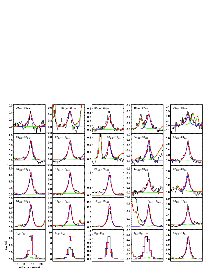
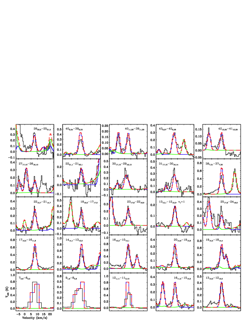
Figure 13.33: Observed transitions in the HIFI and IRAM surveys (black) with the XCLASS model for H₂CS overlaid as a blue solid line. Modeled emission from all other species (solid green) along with the total fit (dashed red) are also overlaid. Quantum numbers labeling each transition are given in each panel and excitation energy increases from the lower left panel to the upper right. See Sec. 5 for a description of the quantum numbers.

We observe thioformaldehyde (H₂CS) emission toward the hot core (s) and compact ridge (Fig. 13.33). In the HIFI scan, we detect emission over a range in $E_{\rm up}$ of $\sim$ 200 – 600 K. While in the IRAM survey, we detect transitions at lower excitation over an $E_{\rm up}$ range of $\sim$ 10 – 200 K. Temperature gradients are not required for either component in our XCLASS model. We derive rotation temperatures of 120 K and 100 K for the hot core and compact ridge, respectively. Tercero et al. (2010) present analysis of the H₂CS emission in the IRAM survey. Despite the fact that they assume a different compact ridge source size (15″) and a different temperature for the hot core (225 K) in their analysis, we derive column densities that agree to within a factor of 2.5. They also derive an ortho/para ratio of $\sim$ 2.0 $\pm$ 0.7 for both the compact ridge and hot core (small variations exist between isotopologues), which, given the uncertainty, is consistent with the equilibrium value of 3. We used a spectroscopic catalog that did not separate the ortho and para species (CDMS catalog) and found that a single ortho + para model fit the data well, which, for the temperatures considered in our models, points to an ortho/para ratio of 3.

5.14 OCS

We observe carbonyl sulfide (OCS) emission toward all spatial/velocity components (Fig. 13.34). In the HIFI and IRAM scans, we detect transitions from J = 40 – 39 to approximately 61 – 60 ($E_{\rm up}$ $\approx$ 480 – 1100 K) and 7 – 6 to 23 – 22 ($E_{\rm up}$ $\approx$ 20 – 160 K), respectively. We do not detect vibrationally excited emission in the HIFI dataset, but do in the IRAM scan ($\nu_{2}$ = 1). Temperature gradients are not needed to fit any component using XCLASS. Our derived rotation temperatures are 190 K for the hot core, 165 K for the compact ridge, 110 K for the plateau, and 10 K for the extended ridge. The OCS emission within the IRAM survey, including the vibrationally excited emission, is analyzed in detail by Tercero et al. (2010). As a result, we do not include a vibrationally excited OCS model here. Our derived column densities agree to within a factor of 2.5 with that derived in the Tercero study.

5.15 SO

Sulfur monoxide (SO) is detected toward the hot core, plateau, and extended ridge (Figs. 13.35 – 13.37). We also observe the rarer isotopologues ³³SO and ³⁴SO toward the hot core and plateau. In the HIFI scan, we detect transitions over a range in $E_{\rm up}$ of $\sim$ 10 – 1200 K. While in the IRAM survey, we detect additional low energy rotation transitions with $E_{\rm up}$ $\lesssim$ 100 K. Using XCLASS, we require temperature gradients to fit both the hot core and plateau. A consistent set of rotation temperatures is adopted for the rarer species. We derive $T_{\rm rot}$ values of 258 K for the hot core, 163 K for the plateau, and 60 K for the extended ridge. Line profiles are dominated by the plateau especially at low excitation. Hence, our reported extended ridge model is not very well constrained because it manifests as a small bump atop the strong plateau component. Our model reproduces the observed line intensities of the $\Delta$N = 1, $\Delta$J = 1 transitions well, which are quite strong in the HIFI scan ($T_{\rm peak}$ values can be as high as 25 K). We, however, note that our model systematically under predicts the less emissive $\Delta$N = 1, $\Delta$J = 0 rotation transitions (observed $T_{\rm peak}$ $\lesssim$ 3 K) by approximately a factor of 5. We even detect several $\Delta$N = 3 lines at the 1 K level, which our model also under predicts. We also fit SO and its isotopologues using MADEX (Figs. 14.13 – 14.15). The plateau is modeled with a temperature/density gradient while the hot core and extended ridge are fit with single components. Our MADEX models also under predict the $\Delta$N = 1, $\Delta$J = 0 and $\Delta$N = 3 transitions. The ³⁴SO MADEX model includes an extended ridge component to fit extremely weak emission in the IRAM survey, which we do not include in the corresponding XCLASS model. Collision rates are taken from Lique et al. (2006), who report rates for He, scaled to H₂. Esplugues et al. (2013a) modeled the emission of SO and its isotopologues within the IRAM survey using MADEX in non-LTE mode. Their column densities, for the rarer isotopologues, agree to within a factor of 3 with our LTE $N_{\rm tot}$ values.

5.16 SO₂

The main isotopologue of sulfur dioxide (SO₂) is observed toward all spatial velocity components (Figs. 13.38 – 13.41). The rarer isotopologues ³³SO₂ and ³⁴SO₂ are also detected toward the hot core and plateau. Additionally, we observe the $\nu_{2}$ = 1 vibrationally excited mode toward the hot core. In the HIFI scan, we detect transitions with $E_{\rm up}$ from $\sim$ 70 K to $\sim$ 1100 K, the most highly excited lines originating from the $\nu_{2}$ = 1 state. The IRAM survey probes excitation energies as low as $\sim$10 K. Modeling the data with XCLASS, we adopt a single set of rotation temperatures for all isotopologues. We derive $T_{\rm rot}$ values of 240 K for the hot core, 100 K for the compact ridge, 150 K for the plateau, and 50 K for the extended ridge. Temperature gradients are required to fit the hot core and compact ridge. We fit the $\nu_{2}$ = 1 emission using the same $T_{\rm rot}$ as the ground vibrational state. We also modeled SO₂ and its isotopologues in the ground vibrational state with MADEX (Figs. 14.16 – 14.18). Unfortunately, collision rates do not exist at high enough excitation to produce reliable non-LTE models at HIFI frequencies. Attempts to use estimated collision rates, moreover, produced suspicious level populations. As a result, the MADEX SO₂ models presented here are computed assuming LTE. Just as with the MADEX SO models, the plateau is fit with a temperature gradient. The hot core, extended ridge, and compact ridge are fit with single temperature models. Our ³³SO₂ and ³⁴SO₂ MADEX fits include compact ridge and extended ridge components to fit extremely weak emission in the IRAM survey, which we do not include in the corresponding XCLASS models. Esplugues et al. (2013a) modeled the emission of SO₂ and its isotopologues within the IRAM survey using MADEX assuming LTE. They derive column densities for the rarer isotopologues that agree to within a factor of 3 with ours.

5.17 HCS⁺

We detect the main isotopologue of thioformylium (HCS⁺) exclusively toward the compact ridge (Fig. 13.42). In the HIFI scan, we observe transitions from J = 12 – 11 ($E_{\rm up}$ = 160 K) to approximately 20 – 19 ($E_{\rm up}$ = 430 K). The IRAM data contains the J = 2 – 1, 4 – 3, and 5 – 4 transitions ($E_{\rm up}$ = 6 – 31 K). All observed HCS⁺ lines in both the IRAM and HIFI scans are weak ($T_{\rm peak}$ $\lesssim$ 1 K). A single temperature model with $T_{\rm rot}$ = 105 K fits the data well. As with the other sulfur carbon molecules detected in this survey, the HCS⁺ emission in the IRAM scan was analyzed using MADEX by Tercero et al. (2010). Our derived column density ($N_{\rm tot}$ = 1.8 $\times$ 10¹⁴ cm^-2) is a factor of $\sim$ 2 times higher than that reported by the Tercero study for the compact ridge. Our results are thus in close agreement with theirs despite our assumption of LTE and the fact that Tercero et al. (2010) assume $\theta_{s}$ = 15″ for the compact ridge, which is likely the biggest reason our HCS⁺ column density is somewhat higher than theirs.

5.18 SiS

We detect the main isotopologue of silicon monosulfide (SiS) toward the plateau (Fig. 13.43). We observe transitions from J = 27 – 26 to approximately 41 – 40 ($E_{\rm up}$ $\approx$ 330 – 750 K) in the HIFI scan, while the IRAM survey contains transitions from J = 5 – 4 to 15 – 14 ($E_{\rm up}$ $\approx$ 10 – 110 K). The observed emission is fit well by a single temperature XCLASS model with $T_{\rm rot}$ = 145 K. Tercero et al. (2011) analyze the SiS emission within the IRAM dataset. In that study, they model the SiS lines by including contributions from the hot core, plateau, and the so called 15.5 km/s component. At HIFI frequencies, we only observe SiS emission from the plateau. As a result, we do not include models for the other two components. The Tercero study derives a column density of 3.5 $\times$ 10¹⁴ cm^-2 toward the plateau using MADEX, not assuming LTE. Our derived column density of 4.3 $\times$ 10¹⁴ cm^-2 thus agrees well with the Tercero result, despite our assumption of LTE.

5.19 SiO

Silicon monoxide (SiO) emission is detected toward the plateau (Figs. 13.44 – 13.46). In addition to the main isotopologue, we also detect emission from ²⁹SiO and ³⁰SiO. The HIFI survey contains transitions from J = 12 – 11 to 29 – 28 ($E_{\rm up}$= 163 – 905 K) and the IRAM scan contains transitions from J = 2 – 1 to 6 – 5 ($E_{\rm up}$= 6 – 44 K). We fit the line emission in XCLASS by splitting the model into high velocity plateau (v_lsr = 10.0 km/s, $\Delta$v = 35 km/s) and low velocity plateau (v_lsr = 7 – 8.0 km/s, $\Delta$v = 15 km/s) components. These two components do not necessarily correspond to the LVF and HVF as defined in Sec. 3.1. Both components require temperature gradients in order to fit both the HIFI and IRAM observations. We were able to adopt a consistent set of rotation temperatures for all isotopologues. We derive $T_{\rm rot}$ values of 120 K and 270 K for the high and low velocity plateau components, respectively. Tercero et al. (2011) modeled the SiO emission in the IRAM survey using MADEX in a similar way. In addition to low and high velocity plateau components, they include hot core, compact ridge, and extended ridge components to fit the line profiles. We do not detect compact or extended ridge components at HIFI frequencies and thus do not include models for those components here. It is, however, possible that the component we attribute to the low velocity plateau may include emission from the hot core. Nevertheless, we find a two component model reproduces the data well. Furthermore, our ²⁹SiO and ³⁰SiO column densities (the sum of all temperature sub-components) are commensurate with those derived in the Tercero study.

5.20 HCl

We observe the J = 1 – 0, 2 – 1, and 3 – 2 transitions of hydrochloric acid (HCl) and H³⁷Cl in the HIFI scan (Figs. 13.47 – 13.48). The line profiles are wide ($\Delta$v = 25 km/s), indicating an origin in the plateau. Because of the wide line profiles, we do not resolve the hyperfine components. The J = 2 – 1 and 3 – 2 lines show blue shifted absorption in both the main and ³⁷Cl isotopologues, while the ground state lines do not. The absorption component appears also to be wide ($\Delta$v $\gtrsim$ 15 km/s), though it is difficult to constrain because of the blending between absorption and emission. The wide line width suggests the absorbing layer also originates from the plateau. We do not fit the absorption component in this work. A temperature gradient is not required to fit the emission and we derive $T_{\rm rot}$ = 73 K for both isotopologues. In order to reproduce the observed peak line intensities, we needed to use a 50″ source size as opposed to 30″, indicating HCl is quite extended toward the plateau. It is also possible that emission from other components, (e.g. the hot core), may be contributing to the line profiles. However, given the dominance of the plateau and the presence of blue shifted absorption in the excited lines, adding such components would not be meaningfully constrained.

5.21 NS

We observe nitric sulfide (NS) emission toward the hot core and compact ridge (Fig. 13.49). In the HIFI scan, we detect NS transitions from J = 21/2 – 19/2 to approximately J = 47/2 – 45/2 ($E_{\rm up}$= 134 – 960 K). In the IRAM survey, we observe emission from the J = 5/2 – 3/2 and J = 7/2 – 5/2 transitions ($E_{\rm up}$ $\approx$ 10 – 340 K), the hyperfine structure being visible in the IRAM scan but not at HIFI frequencies. We, however, do observe the splitting from the unpaired electron in the HIFI spectrum. We did not require temperature gradients for either component in our XCLASS model and derive $T_{\rm rot}$ = 105 and 200 K for the hot core and compact ridge, respectively. We note that our model systematically predicts line centers $\sim$ 10 – 20 MHz higher than observed for many transitions $\gtrsim$ 1 THz. Such differences are commensurate with the quoted uncertainties in the line catalog (JPL database) used to produce the model, which begin to noticeably increase as a function of frequency for $\nu$ $\gtrsim$ 700 GHz.

5.22 NO

We observe nitric oxide (NO) emission toward all spatial/velocity components (Fig. 13.50). In the HIFI scan, we detect transitions from J = 11/2 – 9/2 to approximately J = 29/2 – 27/2 ($E_{\rm up}$ $\approx$ 80 – 540 K). In the IRAM survey, we detect hyperfine lines from the ground state rotation transition J = 3/2 – 1/2. As with the other nitrogen bearing radicals in this survey, we do not detect hyperfine structure in the HIFI scan, but do observe the doublets produced by the spin angular momentum of the unpaired electron. We do not need temperature gradients for any spatial/velocity component and derive $T_{\rm rot}$ values of 180 K for the hot core, 70 K for the compact ridge, 155 K for the plateau, and 60 K for the extended ridge.

5.23 H₂CO

We observe formaldehyde (H₂CO) emission toward the hot core (s), compact ridge, and plateau (Figs. 13.51 – 13.53). We also detect the rarer isotopologue H₂¹³CO toward the hot core (s) and compact ridge, as well as the singly deuterated species, HDCO, only toward the compact ridge. In the HIFI and IRAM surveys, we detect transitions over ranges in excitation energy of $\sim$ 100 – 1000 K and $\sim$ 10 – 90 K, respectively. Single temperature models are used for all spatial/velocity components except the plateau. For H₂CO and H₂¹³CO, we use a source size of 15″ for the compact ridge because models with $\theta_{s}$ = 10″, our standard source size for the compact ridge, predict line intensities that are too weak. We derive $T_{\rm rot}$ values of 135 K for the hot core (s), 50 K for the compact ridge, and 88 K for the plateau. A more detailed analysis of formaldehyde emission in the HIFI scan is presented by Neill et al. (2013a), who use the RADEX non-LTE code (van der Tak et al., 2007) to model the formaldehyde emission toward the compact ridge in order to obtain a robust D/H ratio. As discussed in the Neill et al. (2013a) study, the HDCO line profiles differ somewhat from other compact ridge tracers in that they contain two narrow components (both with $\Delta$v = 2.2 km/s): one at v_lsr = 7.7 km/s, near the canonical velocity of the compact ridge, and the other at v_lsr = 10.0 km/s. The detection of the higher velocity component points to the presence of a highly deuterated clump, the origin of which remains unclear. As a result, our HDCO model contains two velocity components at 7.7 and 10.0 km/s. Both of which assume a source size 12.5″ to remain consistent with Neill et al. (2013a).

5.24 H₂CCO

We detect ketene (H₂CCO) emission only toward the compact ridge (Fig. 13.54). In the HIFI scan, the observed line intensities are quite weak ($T_{\rm peak}$ $<$ 0.5 K). Nevertheless, we detect transitions in the HIFI scan over an approximate range in $E_{\rm up}$ of 300 – 500 K. While in the IRAM survey we observe transitions with excitation energies from $\sim$ 20 K to 150 K. The line profiles in the IRAM scan contain a wider component (v_lsr $\approx$ 6 km/s, $\Delta$v $\approx$ 15 km/s) that we attribute to the hot core. Because this component is only visible in the IRAM data, we do not include a hot core model in this work. We derive $T_{\rm rot}$ = 100 K with no temperature gradient.

5.25 H₂O

We detect water (H₂O) emission toward the hot core (s), compact ridge, and plateau (Figs. 13.55 – 13.61). In addition to the main isotopologue, we also observe H₂¹⁸O, H₂¹⁷O, HDO, HD¹⁸O, and D₂O. Emission from the $\nu_{2}$ = 1 vibrationally excited mode is also detected from the main isotopologue. In the HIFI survey, we detect from the ground state transition up to excitation energies $\gtrsim$ 2500 K, the most highly excited lines originating from $\nu_{2}$ = 1. Absorption is also observed in low energy lines ($E_{\rm up}$ $\lesssim$ 200 K). We derive $T_{\rm rot}$ values of 270, 150, and 150 K for the hot core, compact ridge, and plateau, respectively. More detailed non-LTE analyses of the water emission in the HIFI scan are presented by Melnick et al. (2010) and, more recently, by Neill et al. (2013b), in which water abundances as well as D/H ratios toward the different spatial/velocity components are derived. We adopt the abundances derived in Neill et al. (2013b) here.

5.26 CH₂NH

Methanimine (CH₂NH) is detected toward the hot core and extended ridge (Fig. 13.62). In the HIFI and IRAM scans, we detect transitions over ranges in $E_{\rm up}$ of $\sim$ 15 – 370 K and 5 – 50 K, respectively. Temperature gradients are not required for either component. We derive $T_{\rm rot}$ = 130 and 40 K toward the hot core and extended ridge, respectively.

5.27 NH₂CHO

We observe formamide (NH₂CHO) emission only toward the compact ridge (Fig. 13.63). The HIFI and IRAM scans contain transitions over ranges in excitation energy of approximately 280 – 660 K and 10 – 150 K, respectively. We detect only the more emissive a-type transitions, the b-types having over a factor of 4 lower dipole moment than the a-types. Even at low excitation, the lines are weak ($T_{\rm peak}$ $<$ 0.5 K) in the HIFI survey. There are hints of a wider component in the IRAM scan, possibly from the hot core (see Motiyenko et al., 2012), but we do not include a model for that component here. A single temperature model with $T_{\rm rot}$ = 190 K fits the observed emission well. Motiyenko et al. (2012) model formamide emission within the IRAM survey. They obtain a compact ridge column density that agrees closely (within 10%) with our value. Our derived $T_{\rm rot}$ agrees well with that reported in Sutton et al. (1995), which we used as a starting point for our own fit. Our derived $N_{\rm tot}$ is roughly a factor of $\sim$ 3 higher than that reported in the Sutton study, most likely because Sutton et al. (1995) reports a beam averaged column density for formamide.

5.28 C₂H₅OH

Ethanol (C₂H₅OH) emission is observed toward the compact ridge (Fig. 13.64). In the HIFI and IRAM surveys, we detect transitions over approximate ranges in $E_{\rm up}$ of 100 – 470 K and 30 – 210 K, respectively. We do not need a temperature gradient to fit the observed emission and derive $T_{\rm rot}$ = 110 K. As with several other complex organics detected in this survey, the observed line profiles are weak ($T_{\rm peak}$ $<$ 1 K).

5.29 CH₃OCH₃

Dimethyl ether (CH₃OCH₃) is detected toward the hot core (s) and compact ridge (Fig. 13.65). In the HIFI and IRAM scans, we observe transitions over ranges in excitation energy of $\sim$ 90 – 620 K and 5 – 510 K, respectively. Single temperature models are sufficient to fit both components. We derive $T_{\rm rot}$ = 100 and 110 K for the hot core (s) and compact ridge, respectively.

5.30 CH₃OCHO

We observe methyl formate (CH₃OCHO) only toward the compact ridge (Fig. 13.66). Transitions in the HIFI and IRAM surveys are detected over $E_{\rm up}$ ranges of $\sim$ 160 – 740 K and 10 – 300 K, respectively. A fraction of the detected lines are from the v_t = 1 torsionally excited state. Favre et al. (2011) observe multiple transitions of CH₃OCHO using the Plateau de Bure Interferometer (PdBI). In that study, they fit the observed line profiles using two velocity components, one at v_lsr = 7.5 km/s and the other at 9.2 km/s, both of which have $\Delta$v = 1.7 km/s. We find that a single compact ridge model with v_lsr = 8.0 km/s, $\Delta$v = 2.8 km/s, and $T_{\rm rot}$ = 110 K reproduces the HIFI observations well, though some line profiles hint at the possibility for two components. When both velocity components are combined, our derived $T_{\rm rot}$ agrees well with theirs toward MF1 ($T_{\rm rot}$ = 100 K), the largest methyl formate clump observed toward the compact ridge. Our derived column density is also commensurate with that derived by Favre et al. (2011) toward MF1.

5.31 CH₃OH

We observe methanol (CH₃OH) emission toward the hot core (s) and compact ridge (Figs. 13.67 – 13.72). In addition to the main isotopologue, we also detect ¹³CH₃OH as well as the singly deuterated CH₃OD and CH₂DOH isotopologues toward these same spatial/velocity components. In both the HIFI and IRAM surveys, we detect transitions over a range in excitation energy of approximately 20 – 1200 K, the most highly excited transitions originating from the torsionally excited $\nu_{t}$ = 1 mode. We derive $T_{\rm rot}$ = 128 and 140 K for the hot core (s) and compact ridge, respectively. More detailed analysis of methanol emission within the HIFI scan is presented by Wang et al. (2011) and Neill et al. (2013a).

5.32 HF

The J = 1 – 0 transition of hydrogen fluoride (HF) is detected in the HIFI scan (Fig. 13.73), but is heavily blended with transitions of SO₂ and CH₃OH. After subtracting emission from contaminating lines, Phillips et al. (2010) finds the HF 1 – 0 transition displays a strong blue shifted absorption component, which extends over a v_lsr range of $\sim$ $-$9 – $-$45 km/s, and a weaker red shifted emission component which extends over a v_lsr range of $\sim$ 12 – 50 km/s. The broad line profile indicates an origin in the plateau. Phillips et al. (2010) estimates an HF column density in the absorption component, which they attribute to the LVF, of 2.9 $\times$ 10¹³ cm^-2. Because we only observe the ground state and the line profile is dominated by absorption, we do not provide an HF model.

5.33 CO

We observe CO, ¹³CO, C¹⁸O, and C¹⁷O toward all spatial/velocity components and ¹³C¹⁸O toward the extended ridge and compact ridge (Figs. 13.74 – 13.78). In the HIFI scan, we detect transitions from 5 – 4 up to 17 – 16 ($E_{\rm up}$ = 80 – 810 K), while the IRAM survey contains the 1 – 0 ground state transition. Our reported $T_{\rm rot}$ values are the same as those used in Plume et al. (2012), who analyze the C¹⁸O and C¹⁷O emission in the HIFI scan to obtain robust H₂ column density measurements toward the different spatial/velocity components within Orion KL, except for the plateau, toward which we use a higher $T_{\rm rot}$. These $T_{\rm rot}$ values are 150 K for the hot core, 125 K for the compact ridge, 130 K for the plateau, and 40 K for the extended ridge. As described in Sec. 3.3, we adopt these $N_{\rm H_{2}}$ estimates in this study modulo small adjustments for the plateau and compact ridge. With this said, we note that our reported plateau C¹⁸O column density is higher by a factor of 1.8 than the $N_{\rm H_{2}}$ value given in Table 2 multiplied by 2.0 $\times$ 10^-7, our assumed C¹⁸O abundance. The reason for this discrepancy is that a somewhat wider plateau line width ($\Delta$v = 25 km/s) than used in the Plume study ($\Delta$v = 20 km/s) appears to produce better agreement between the model and data. As a result, we were forced to increase the C¹⁸O column density by a factor of 1.8 to properly fit the data.

5.34 NH₂

Only the ortho species of amidogen (NH₂) is detected toward the hot core and extended ridge (Fig. 13.79). In the HIFI scan, we detect from the ground state up to excitation energies of $\sim$ 375 K. No transitions are detected in the IRAM survey. We derive $T_{\rm rot}$ = 130 and 50 K toward the hot core and extended ridge, respectively.

5.35 NH₃

We observe ammonia (NH₃) toward the hot core, plateau, and extended ridge (Figs. 13.80 – 13.84). We also detect ¹⁵NH₃ and NH₂D as well as the $\nu_{2}$ = 1 vibrationally excited mode from the main isotopologue. Emission from the $\nu_{2}$ = 1 mode and NH₂D are only detected toward the hot core. The main and ¹⁵N isotopologues are observed via low energy rotation transitions which include the ground state ortho and para lines up to the 3₀ – 2₀ ortho transition ($E_{\rm up}$ $\approx$ 170 K). Because the deuterium atom breaks the symmetry of the ammonia molecule, we observe NH₂D transitions within and across K ladders up to excitation energies of $\sim$ 600 K. Vibrationally excited emission is detected from energy levels as high as $\sim$ 2000 K. A detailed analysis of the NH₂D emission in the HIFI scan is presented by Neill et al. (2013a) for the purpose of obtaining a robust ammonia D/H ratio. The observed NH₃ and ¹⁵NH₃ transitions do not cover a large range in excitation energy. The lines from the main isotopologue, moreover, have a blue shifted absorption component, which we do not fit here. Consequently, we derive a $T_{\rm rot}$ = 250 K toward the hot core based on the $\nu_{2}$ = 1 and NH₂D emission. We also derive $T_{\rm rot}$ = 23 and 35 K for the extended ridge and plateau, respectively, though these values are not as well constrained because of the limited coverage in excitation energy. Because of the limited coverage in $E_{\rm up}$, we do not report NH₃ abundances in this work.

5.36 OH

We observe the hydroxyl radical (OH) toward the plateau and the deuterated isotopologue (OD) toward the compact ridge (Figs. 13.85 – 13.86). For both species, we detect only the ${}^{2}\Pi_{1/2}$ J = 3/2 – 1/2 doublet in the HIFI scan. We used $T_{\rm rot}$ =125 K, characteristic of the compact ridge, to fit the OD lines. We, however, note that this rotation temperature is not well constrained because only one $E_{\rm up}$ is sampled.

5.37 CH⁺

We detect the J = 2 – 1 transition of methyliumylidene (CH⁺) in absorption (Fig. 13.87). The line profile has a v_lsr $\approx$ 8 km/s and $\Delta$v $\approx$ 5 km/s indicating a possible origin in the extended ridge, though the measured $\Delta$v is slightly wider than typical for this spatial/velocity component. We possibly detect the J = 1 – 0 transition with both emission and absorption components, although it is not clear because the baseline is irregular at this frequency. Because of the small $E_{\rm up}$ coverage and the fact that this species is detected in absorption, we do not include a model for CH⁺.

5.38 H₂O⁺

We detect the ortho ground state rotation transition (1_1,1 – 0_0,0) of the water cation (H₂O⁺) in absorption (Fig. 13.88). Both fine structure components, J = 3/2 – 1/2 and J = 1/2 – 1/2, are detected but the latter is heavily blended with emission lines from other species. As discussed by Gupta et al. (2010), who analyze the H₂O⁺ emission in detail, the J = 3/2 – 1/2 transition contains a narrow absorption component at v_lsr $\sim$ 9 km/s consistent with the extended ridge. The J = 3/2 – 1/2 transition also displays a broad blue-shifted absorption component that extends to v_lsr $\sim$ $-$45 km/s, similar to the J = 1–0 transition of HF (see Phillips et al., 2010), which likely originates from the LVF. Gupta et al. (2010) derive column densities of 7 $\pm$ 2 $\times$ 10¹² cm^-2 and 1.0 $\pm$ 0.3 $\times$ 10¹³ cm^-2 for the narrow and broad components, respectively. Because of the small $E_{\rm up}$ coverage and the fact that this molecule is only detected in absorption, we do not provide an H₂O⁺ model.

5.39 OH⁺

We detect the ground state rotation transition of the hydroxyl cation (OH⁺) in absorption (Fig. 13.89). The J = 1 – 1 and 2 – 1 fine structure components are clearly detected, while the J = 0 – 1 component is heavily blended. Gupta et al. (2010) analyze the OH⁺ emission in detail. They find that the OH⁺ lines are similar to those of H₂O⁺ and HF, and contain both a narrow component at v_lsr $\sim$ 9 km/s, consistent with the extended ridge, and a wider blue-shifted component which originates in the LVF. Gupta et al. (2010) derive column densities of 9 $\pm$ 3 $\times$ 10¹² cm^-2 and 1.9 $\pm$ 0.7 $\times$ 10¹³ cm^-2 for the narrow and broad components, respectively. Because of the small $E_{\rm up}$ coverage and the fact that this molecule is only detected in absorption, we do not provide an OH⁺ model.

5.40 Atomic Species

We detect the ${}^{3}P_{1}$ – ${}^{3}P_{0}$ and ${}^{3}P_{2}$ – ${}^{3}P_{1}$ transitions of neutral atomic carbon (CI, Fig. 13.90) and the ${}^{2}P_{3/2}$ – ${}^{2}P_{1/2}$ transition of singly ionized carbon (CII, Fig. 13.91). The CI and CII line profiles contain emission and absorption components. There are at least two emission components in the CI profiles: one wide (v_lsr $\sim$ 8.5 km/s, $\Delta$v $\sim$ 13 km/s), suggesting an origin in the plateau or hot core (s), and one more narrow (v_lsr $\sim$ 7.5 km/s, $\Delta$v $\sim$ 3 km/s), indicating emission from the compact ridge. In the CI lines, the absorption component has v_lsr $\sim$ 11.5 km/s and $\Delta$v $\sim$ 2 km/s, suggesting absorption from the extended ridge. The CII line also contains at least two emission components possibly originating from the plateau (v_lsr $\sim$ 7.5 km/s, $\Delta$v $\sim$ 17 km/s) and compact ridge (v_lsr $\sim$ 8.0 km/s, $\Delta$v $\sim$ 4 km/s). The absorption component in the CII line is more prominent than in the CI transitions, and is wider (v_lsr $\sim$ 8.0 km/s, $\Delta$v $\sim$ 6 km/s) than what is typical for the extended ridge. Atomic emission toward Orion KL is more extended than the DBS mode 3′ chopper throw (see e.g. Werner et al., 1984; Genzel & Stutzki, 1989; Herrmann et al., 1997; Ikeda et al., 1999, 2002). Emission in the off beam, therefore, likely contributes to some of the perceived absorption observed in the CI and CII lines. Lastly, we do not detect the ${}^{3}P_{1}$ – ${}^{3}P_{0}$ transition of NII at 1461.1 GHz. Because of the off beam contamination and the fact that we are focused on molecular emission in this study, we do not include models for CI and CII.

6 Discussion

The $\chi_{\rm red}^{2}$ values reported in Table 6, in general, indicate excellent agreement between the data and models. Most of the complex organics, in particular, have low $\chi_{\rm red}^{2}$ values ($\lesssim$ 1.5), indicating LTE is a good approximation for these species and suggests an origin in high density gas ($>$ 10⁶ cm^-3). As a result, abundances of complex molecules derived from our LTE fits should be robust estimates toward Orion KL. The fact that CH₃CN abundances derived from our XCLASS and more advanced non-LTE models agree closely with one another supports this assertion. LTE models, therefore, may be sufficient to derive robust abundances for complex organics toward other massive hot cores, where gas densities are high. The exceptions to this are some isotopologues (including the main isotopologue) of methanol and the $\nu_{8}$ = 1 CH₃CN model which have $\chi_{\rm red}^{2}$ $\geq$ 3.5. These high $\chi_{\rm red}^{2}$ values are likely due to a combination of issues brought on by high optical depth, non-LTE excitation, and radiative pumping (see Sec. 4.1).

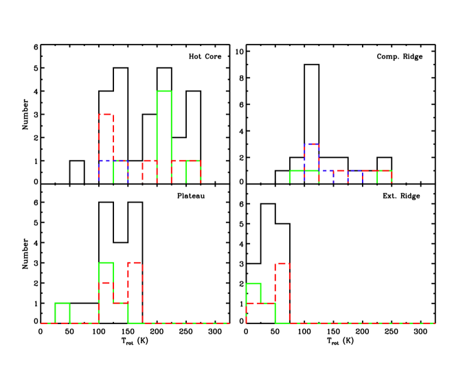
Figure 20: Rotation temperature histograms originating from the individual spatial/velocity components. Rotation temperatures from cyanides, sulfur bearing molecules, and complex oxygen bearing organics are plotted as solid green, dashed red, and dashed blue lines, respectively. $T_{\rm rot}$ values from all molecules are plotted as a black solid line.

In addition to molecular abundances, our XCLASS models provide rotation temperatures for each species, which, under the assumption of LTE, estimates the local gas kinetic temperature. The distribution of rotation temperatures toward each spatial/velocity component therefore yields insight into the thermal structure within each region. Fig. 20 shows histograms of rotation temperature in four panels, each representing a different spatial/velocity component. For molecules fit with temperature gradients, we only include the $T_{\rm rot}$ which corresponds to the sub-component that dominates the emission in the HIFI survey. Species with multiple detected isotopologues are only counted once. We exclude rotation temperatures derived for NH₃ toward the plateau and extended ridge, as well as OD toward the compact ridge because they were fit using transitions over a small range in $E_{\rm up}$ (see Secs. 5.35 and 5.36). Within each panel, the black solid curve corresponds to the $T_{\rm rot}$ distribution of all molecules detected toward that component. The solid green, dashed red, and dashed blue lines represent cyanides, sulfur bearing molecules, and complex oxygen bearing organics, respectively. More discussion on the chemical implications of our results will be given in a future work (Crockett et al. 2014, in preparation).

Examining Fig 20, we see the spread in rotation temperature is much larger toward the hot core relative to the other spatial/velocity components, suggesting the hot core has the most heterogeneous thermal structure toward Orion KL. In particular, there are a significant number of hot core molecules with $T_{\rm rot}$ $>$ 175 K, which is where the other distributions, (save a few species in the compact ridge), terminate. Interferometric studies of molecular emission toward the hot core have certainly demonstrated that this region is both chemically and physically intricate, having structure on scales $\lesssim$ 1-2″ (Wang et al., 2010; Goddi et al., 2011). Examining which molecules have the highest $T_{\rm rot}$ toward the hot core, we see that cyanides (green histogram) account for 5 of the 11 molecules with $T_{\rm rot}$ $>$ 200 K. We note the cyanide in the 125 – 150 K bin, C₂H₅CN with $T_{\rm rot}$ = 136 K, requires an additional compact 300 K sub-component to fit lines at high excitation. In general, sulfur bearing molecules do not have particularly high rotation temperatures toward the hot core, although S-bearing species which also contain oxygen (i.e. OCS, SO, and SO₂) all have rotation temperatures $>$ 175 K.

It is possible that the hot core $T_{\rm rot}$ distribution is influenced by radiative pumping from the strong IR continuum characteristic of this region (Genzel & Stutzki, 1989; De Buizer et al., 2012). Detailed non-LTE studies of emission from H₂O (Neill et al., 2013b) and H₂S (Crockett et al., 2014) within the Orion KL HIFI scan require an enhanced far-IR continuum ($\lambda$ $<$ 100 $\mu$m) compared to what is observed to explain the emission of both these light hydrides. Because much of the far-IR is optically thick, this suggests a possible origin near a hidden self-luminous source or sources. Other studies have also needed to invoke strong IR radiation fields to explain NH₃ (Hermsen et al., 1988) and HDO (Jacq et al., 1990) emission toward the hot core. We note that all hot core tracers with detected vibrational modes, except CH₃OH, have rotation temperatures $>$ 175 K. Most of these vibrationally excited modes are likely populated via pumping from the mid/far-IR. Thus it is possible that the local radiation field is redistributing the population levels of these molecules to reflect a higher $T_{\rm rot}$ than the actual kinetic temperature.

The compact ridge $T_{\rm rot}$ distribution is much narrower than that of the hot core with a little less than half of the distribution falling in the 100 – 125 K bin, indicating a more quiescent, uniform environment. Most of the complex O-bearing molecules have rotation temperatures near the peak of this distribution, with the exception of NH₂CHO which has $T_{\rm rot}$ = 190 K. There are, however, several high temperature outliers. Just as in the hot core, CH₃CN and OCS are on the high end of the $T_{\rm rot}$ distribution. Unlike the hot core, HCN and HNC do not appear to be particularly warm ($T_{\rm rot}$ = 120 K and 80 K, respectively). The other species populating the high temperature part of the compact ridge distribution are NS and CS, both of which do not have particularly high $T_{\rm rot}$ values toward the hot core ($T_{\rm rot}$ $\approx$ 100 K).

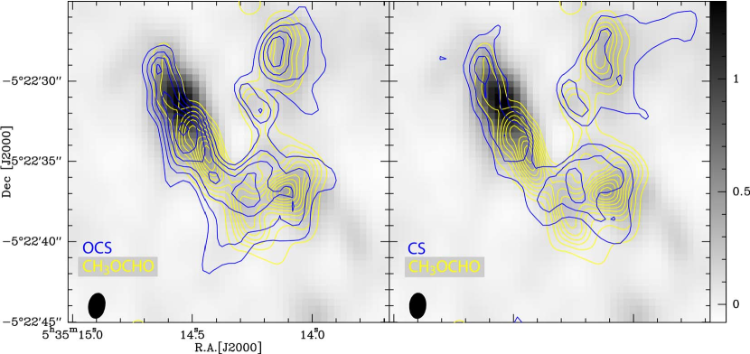
Figure 21: Integrated intensity maps of OCS 20 – 19 and CS 5 – 4 between v_lsr = 7.6 – 8.3 km/s (blue contours) from the ALMA-SV survey. The first contour corresponds to 1.32 Jy beam^-1 km s^-1 and higher contours increase in steps of 1.28 Jy beam^-1 km s^-1. The yellow contours in both panels correspond to a channel map of CH₃OCHO 18_7,11 – 17_7,10 at v_lsr = 7.8 km/s. The first contour is 337 mJy beam^-1, which is also contour step. The continuum at 230.9 GHz in Jy beam^-1 is overlaid as a greyscale.

To determine if these higher $T_{\rm rot}$ molecules correspond to a spatially distinct region within the compact ridge, we once again employ the ALMA-SV line survey. Emission from two molecules which have high $T_{\rm rot}$ measurements toward the compact ridge, OCS ($T_{\rm rot}$ = 165 K) and CS ($T_{\rm rot}$ = 225 K), are present in the ALMA scan. Fig. 21 plots integrated emission maps of the OCS 20 – 19 and CS 5 – 4 in the left and right panels as blue contours, respectively. The emission is integrated between v_lsr = 7.6 – 8.3 km/s to avoid contributions from the hot core and plateau. We also overlay emission from CH₃OCHO 18_7,11 – 17_7,10, in both panels as yellow contours. Methyl formate is a prominent compact ridge tracer with a derived $T_{\rm rot}$ = 110 K, close to the peak of the compact ridge $T_{\rm rot}$ distribution. The CH₃OCHO contours surround a cavity that is likely carved out by the LVF (Irvine et al., 1987; Plambeck et al., 2009; Favre et al., 2011). The two southern methyl formate peaks, furthermore, correspond to MF1 and MF3 using the labeling conventions of Favre et al. (2011). The continuum is also overlaid on both panels as a gray scale, which mainly traces IRc2, the infrared source closest to the hot core. From the plot, we see that both the OCS and CS peaks are offset from MF1 and MF3, occurring midway between the two and closer to the edge of the CH₃OCHO cavity. The higher rotation temperatures may therefore be a result of the interactions between the LVF and the compact ridge.

The plateau has a narrower $T_{\rm rot}$ distribution than the hot core. Although not as centrally peaked as the compact ridge, the plateau does not have a conspicuous high temperature ($>$ 175 K) tail in its distribution. Unlike the hot core, cyanides are not among the hottest molecules detected toward this component. Although we note torsionally excited CH₃CN emission is observed toward the plateau, from which we compute a vibration temperature of 171 K (see Sec. 4.3). This indicates methyl cyanide may be probing hotter material toward the plateau than the rotation temperature ($T_{\rm rot}$ = 120 K) would suggest. As with the hot core, sulfur bearing species are spread throughout the distribution with the hottest being the O/S-bearing species SO and SO₂. OCS, on the other hand, traces somewhat cooler gas. We note that the highest $T_{\rm rot}$ molecule detected toward the plateau is HNCO ($T_{\rm rot}$ = 168 K), which also displays one of the highest rotation temperatures toward the hot core ($T_{\rm rot}$ = 209 K). This is likely the result of pumping from the far-IR, which Churchwell et al. (1986) has shown is significant for this molecule (see Sec. 5.8).

Finally, the extended ridge displays the narrowest of all four temperature distributions centered at $\sim$ 40 K, exemplifying the cool, quiescent nature of this region. Although there is not much variation in $T_{\rm rot}$, sulfur bearing molecules tend to be warmer than average. Cyanides, on the other hand, are on the cooler side of the distribution.

7 Conclusions

We have presented a full band analysis of the HIFI spectral survey toward Orion KL, which spans a frequency range from 480 to 1907 GHz. In all, we detect emission from 39 molecules (79 isotopologues). Combining this dataset with a ground based mm line survey, we modeled the molecular emission using the XCLASS program, which assumes LTE level populations. A subset of the molecules detected in this survey was also modeled using the MADEX non-LTE code. A $\chi_{\rm red}^{2}$ analysis demonstrates that there is excellent agreement between the data and models for most molecules. In particular, complex organics are well fit by our LTE models, which indicates these species are emitting from high density gas ($n_{\rm H_{2}}$ $>$ 10⁶ cm^-3). According to our LTE fits, we detect $\sim$ 13,000 lines in the HIFI scan and estimate a U line fraction of 12%. Methanol is the most emissive molecule in the HIFI survey both in terms of total integrated intensity and number of detected lines. We detect vibrationally/torsionally excited emission from 10 species and find evidence for radiative pumping of HCN in the hot core and CH₃CN in the plateau. We also isolate a spatial/velocity component that has line parameters “in between” that expected from the hot core and compact ridge ($\Delta$v $\sim$ 5 – 10 km/s, v_lsr $\sim$ 6.5 – 8 km/s), which likely peaks $\sim$ 1″ south of the hot core sub-mm continuum peak consistent with the high water column density clump discovered by Neill et al. (2013b).

Using column densities derived from our models, we computed molecular abundances toward the hot core, compact ridge, plateau, and extended ridge. Abundances derived from our XCLASS and more advanced MADEX models typically agree to within a factor of 3, indicating our LTE abundances are reliable. Plotting the distribution of rotation temperatures toward each spatial/velocity component reveals the HIFI scan probes a diversity of environments toward Orion KL. The $T_{\rm rot}$ distribution for the hot core is significantly wider than the others, suggesting the hot core harbors a more complex thermal structure than the other spatial/velocity components. Although the compact ridge $T_{\rm rot}$ distribution is quite narrow, it does have a high temperature tail. Interferometric maps of OCS and CS, two molecules at the high temperature end of the compact ridge distribution, show these molecules peak closer to the LVF than CH₃OCHO, a species with a rotation temperature near the peak of the compact ridge $T_{\rm rot}$ distribution. The higher temperature tail thus may be the result of interactions between the LVF and compact ridge. The relative and absolute abundances derived in this study, along with the publicly available data and molecular fits, which extend from below 100 GHz to beyond 1.9 THz, represent a legacy for comparison to other sources and chemical models.

Appendix A Reduced $\chi^{2}$ Calculations and Uncertainty Estimates

We calculate reduced chi squared, $\chi_{\rm red}^{2}$, statistics for each model which are reported in Table 6. This calculation is performed by first uniformly smoothing the data to a velocity resolution of $\sim$ 0.5 km/s. Residuals between the molecular fits and data are then computed by stepping across the spectrum in frequency intervals corresponding roughly to 1000 km/s. At each interval, we calculate the RMS noise level and subtract a local baseline. For a channel to be included in the $\chi_{\rm red}^{2}$ calculation of a given molecular fit, the model emission has to be $>$ 3 times the local RMS and responsible for 95% of the total flux when compared to the entire full band model. That is, the intensity ratio between the fit being considered and the full band model has to be $\geq$ 0.95 in order to avoid channels that contain emission from more than one molecule (i.e. blended lines). The uncertainty in each channel, $\sigma_{tot}$, is computed by adding in quadrature the contributions from several different sources of error,

$$\sigma_{tot}=\sqrt{\sigma_{bl}^{2}+\sigma_{rms}^{2}+\sigma_{cal}^{2}+\sigma_{pt}^{2}+\sigma_{bf}^{2}+\sigma_{\tau_{d}}^{2}}.$$ (A1)

Here, $\sigma_{bl}$ is a baseline offset uncertainty, $\sigma_{rms}$ is the local RMS noise level, $\sigma_{cal}$ is the calibration uncertainty, $\sigma_{pt}$ is the pointing error, and $\sigma_{bf}$ is the error in beam filling factor brought on by the source size uncertainty, and $\sigma_{\tau_{d}}$ is the error due to our uncertainty in the dust optical depth. The method used to compute each source of error is given below. All uncertainties are propagated using the “error propagation equation” of Bevington & Robinson (2003, their Eq. 3.13),

$\bm{\sigma_{bl}}$ – This represents offsets in the baseline that still exist despite having subtracted a baseline within each 1000 km/s interval. These offsets exist at approximately the 0.05 K level, we thus take $\sigma_{bl}$ = 0.05 K.

$\bm{\sigma_{rms}}$ – This is the RMS noise level in the baseline. Emission line channels are rejected by excluding channels predicted to be in emission by the full band model. We also use a sigma clip algorithm to remove any additional channels in emission from U lines.

$\bm{\sigma_{cal}}$ – We assume a 10% calibration uncertainty for each channel (Roelfsema et al., 2012).

$\bm{\sigma_{pt}}$ – The pointing uncertainty is computed assuming a Gaussian beam and the nominal Herschel absolute pointing error (APE) of 2″ (Pilbratt et al., 2010). The percent error in the intensity of each channel brought on by the APE, $\delta_{p}$, is thus,

$$\delta_{p}=1-exp\left[-~{}\frac{APE^{2}}{2(\theta_{b}/2.355)^{2}}\right],$$ (A2)

where $\theta_{b}$ is the beam size.

$\bm{\sigma_{bf}}$ – Because we do not vary the source size in our molecular fits, we include a beam filling factor uncertainty. We take the error in source size to be 20%. Assuming the shape of the telescope beam and source are Gaussian, the beam filling factor, $\eta_{bf}$, is,

$$\eta_{bf}=\frac{\theta_{s}^{2}}{\theta_{s}^{2}+\theta_{b}^{2}}.$$ (A3)

The beam filling factor is directly proportional to the observed intensity. Propagating the uncertainty, we derive an expression for the percent error in the intensity of each channel due to our assumed $\theta_{s}$ uncertainty, $\delta_{ss}$,

$$\delta_{ss}=2\ \eta_{bf}(1-\eta_{bf})\frac{\sigma_{s}}{\theta_{s}}$$ (A4)

where $\sigma_{s}$ is the error in the source size and $\sigma_{s}$ / $\theta_{s}$ is the percent error in the source size. In instances when more than one spatial/velocity component is detected for a given species, an intermediate “effective” source size, $\theta_{eff}$, is used for the $\theta_{s}$ in Eq. A3. Adopted $\theta_{eff}$ values are given in Table 6.

$\bm{\sigma_{\tau_{d}}}$ – We find that extinction due to dust significantly reduces the observed line profiles particularly at high frequencies ($\gtrsim$ 800 GHz). We account for the uncertainty in $\tau_{d}$ by assuming a 1 $\sigma$ error of 30% in $N_{\rm H_{2}}$ and propagating this uncertainty using Eq. 1. This is the same error assumed by Crockett et al. (2014), and encompasses $N_{\rm H_{2}}$ values reported in various studies (Plume et al., 2012; Favre et al., 2011; Mundy et al., 1986; Genzel & Stutzki, 1989) at the 3 $\sigma$ level when we set $N_{\rm H_{2}}$ = 2.5 $\times$ 10²⁴ cm^-2 (see Sec. 3.3). The observed main beam temperature goes as $T_{\rm mb}$ $\propto$ $e^{-\tau_{d}}$, the percent error due to $\tau_{d}$ is thus equal to $\sigma_{\tau_{d}}$.

Our derived column densities are based on optically thin emission, which, in this limit, is directly proportional to the observed intensity. The uncertainty in $T_{\rm mb}$ is given by Eq. A1. We note that, in our XCLASS models, line intensity is also a function of rotation temperature. However, for most molecules, we observe transitions over a comprehensive range in excitation energy. As a result, we are able to reasonably decouple $N_{\rm tot}$ and $T_{\rm rot}$ from one another. We estimate an $N_{\rm tot}$ uncertainty of 25% for XCLASS, which we compute using Eq. A1 at 1 THz assuming the sources of error given above. This value is consistent with $N_{\rm tot}$ uncertainties estimated in previous studies which use MADEX to model the Orion KL IRAM survey (Marcelino et al. 2014, in preparation; Tercero et al., 2010, 2011; Esplugues et al., 2013a, b). Because the modeling methodology is similar here, we adopt the same $N_{\rm tot}$ 25% error for MADEX. Applying the same calculation (using Eq. A1 at 1 THz) to Table 7, we estimate a 25% error in the integrated intensities reported for individual spatial/velocity components. We note that this uncertainty may be an underestimate for molecular fits with high $\chi_{\rm red}^{2}$ values (i.e. $\chi_{\rm red}^{2}$ $>$ 3.0, see Sec. 4.1).

We estimate a 10% uncertainty for $T_{\rm rot}$ in our XCLASS models. This uncertainty is commensurate with the $T_{\rm rot}$ percent error derived by Crockett et al. (2014) for H₂S, who report $T_{\rm rot}$ = 141 $\pm$ 12 K, yielding a percent error of 9%. We take this uncertainty as representative of all molecular species and note that changes of 10% in $T_{\rm rot}$ produce noticeable deviations by eye in models that fit the data well.

We adopt errors in the v_lsr values reported in Tables 4 and 5 of $\pm$ 1 km/s for the hot core, compact ridge, and extended ridge, and $\pm$ 2 km/s for the plateau. We also estimate $\Delta$v uncertainties of $\pm$ 0.5 km/s, 1.5 km/s, and 5.0 km/s, for the compact/extended ridge, hot core, and plateau, respectively. These uncertainties are derived by visual comparison of the models and data. Changing the v_lsr or $\Delta$v by increments equal to or greater than these uncertainties produce noticeable differences in model line profiles. The errors are smaller for spatial/velocity components with narrower line profiles because variations in $\Delta$v and v_lsr are more easily detected in these “sharper” components. We note that our uncertainty estimates for $\Delta$v and v_lsr toward each spatial/velocity component are also commensurate with the standard deviation of these quantities for all molecules detected toward each component.

We estimate a 40% error in molecular abundance. We arrive at this value by assuming a 25% error in column density, a 30% error in $N_{\rm H_{2}}$, and propagating the uncertainty, which amounts to adding these quantities in quadrature with one another.

$T_{\rm vib}$ errors reported in Table 9 are computed assuming a 25% error in the column density of each vibrational mode and using Eq. 4 to propagate the uncertainties.

Fig. Set13. Individual XCLASS models

Figure 13.13: Observed transitions in the HIFI and IRAM surveys (black) with the XCLASS model for H¹³CN overlaid as a blue solid line. Modeled emission from all other species (solid green) along with the total fit (dashed red) are also overlaid. Quantum numbers labeling each transition are given in each panel and excitation energy increases from the lower left panel to the upper right. See Sec. 5 for a description of the quantum numbers.

Figure 13.66: Observed transitions in the HIFI and IRAM surveys (black) with the XCLASS model for CH₃OCHO overlaid as a blue solid line. Modeled emission from all other species (solid green) along with the total fit (dashed red) are also overlaid. Quantum numbers labeling each transition are given in each panel and excitation energy increases from the lower left panel to the upper right. See Sec. 5 for a description of the quantum numbers.

Fig. Set14. Individual MADEX models

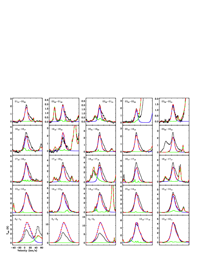
Figure 14.14: Observed transitions in the HIFI and IRAM surveys (black) with the MADEX model for ³⁴SO overlaid as a blue solid line. Modeled emission from all other species (solid green) along with the total fit (dashed red) are also overlaid. Quantum numbers labeling each transition are given in each panel and excitation energy increases from the lower left panel to the upper right. See Sec. 5 for a description of the quantum numbers.

Figure 19: Histogram of the number of U lines as a function of frequency (top) and the fraction of U line channels as a function of frequency (bottom). Both histograms have a bin width of 181 GHz.

Table 1: HIFI Observations

Band	Observation Date	OD	OBSID	Frequency Range	RMS
				(GHz)	(mK)
1a	1 March 2010	291	1342191504	479.5 – 561.5	20
1b	2 March 2010	292	1342191592	554.5 – 636.5	20
2a	12 April 2010	333	1342194540	626.0 – 726.0	20
2b	7 March 2010	297	1342191755	714.1 – 801.3	30
3a	29 September 2010	504	1342205334	799.0 – 860.0	40
3b	19 March 2010	309	1342192329	858.1 – 961.0	40
4a	2 March 2010	293	1342191601	949.1 – 1061.0	50
4b	3 March 2010	294	1342191649	1049.9 – 1122.0	80
5a	6 March 2010	296	1342191725	1108.1 – 1242.8	100
5b	19 March 2011	674	1342216387	1227.1 – 1280.0	100
6a (HC)	6 March 2010	296	1342191727	1425.9 – 1535.0	700
6b (HC)	22 March 2010	312	1342192562	1573.3 – 1702.8	800
7a (HC)	15 April 2010	336	1342194732	1697.2 – 1797.8	800
7b (HC)	23 March 2010	313	1342192673	1788.4 – 1906.5	800
6a (CR)	6 March 2010	296	1342191728	1425.9 – 1535.0	700
6b (CR)	22 March 2010	312	1342192563	1573.3 – 1702.8	800
7a (CR)	15 April 2010	336	1342194733	1697.2 – 1797.8	800
7b (CR)	23 March 2010	313	1342192674	1788.4 – 1906.5	800

Table 2: Adopted Values for Source Size and H₂ Column Density

Component	$\theta_{s}$ (″)	$N_{\rm H_{2}}$ (cm-2)
Hot Core	10	3.1 $\times$ 1023
Compact Ridge	10	3.9 $\times$ 1023
Plateau	30	2.8 $\times$ 1023
Extended Ridge	180	7.1 $\times$ 1022

Note. — Values for $\theta_{s}$ and $N_{\rm H_{2}}$, including references, are explained in Sec. 3.3

Table 3: Optically Thick Molecules

Molecule	Hot Core	Compact Ridge	Plateau	Extended Ridge
CH3CN	X	X	X	…
CH3OH	X	X	…	…
13CO	X	X	X	X
CS	X	X	X	X
H2CO	X	X		…
H218O	X	X	X	…
H2S	X	…	X
HCN	X	X	X	X
HCN,$\nu_{2}$=1	X	…	…	…
H13CN	X		X	X
HCO+	X	X	X	X
HNC	X		X	X
HNCO	X	…	X	…
NH3	X	…	X	X
OH	…	…	X	…
SiO	…	…	X	…
SO	X	…	X
SO2	X		X

Note. — “X” indicates an optically thick model, “…” corresponds to a non-detection, and no mark indicates an optically thin model, which will have an entry in Table 4 and possibly Table 5.

Table 4: XCLASS Model Parameters

Molecule	$\theta_{s}$ (″)	$T_{\rm rot}$ (K)	$N_{\rm tot}$ (cm-2)	vlsr (km/s)	$\Delta$v (km/s)
Hot Core
C2H3CN	20	130	7.5$\times 10^{14}$	3.5	12.5
C2H3CN	10	215	2.7$\times 10^{15}$	5.0	5.5
C2H5CN	10	136	2.1$\times 10^{16}$	5.0	7.0
C2H5CN	5	300	6.5$\times 10^{15}$	5.0	7.0
CH2NH	10	130	1.3$\times 10^{15}$	6.0	8.0
CH3CN,$\nu_{8}$=1	10	260	3.7$\times 10^{15}$	6.0	6.0
13CH3CN	20	80	8.0$\times 10^{13}$	5.5	8.0
13CH3CN	10	260	1.3$\times 10^{14}$	5.5	8.0
CH313CN	20	80	8.0$\times 10^{13}$	5.5	8.0
CH313CN	10	260	1.3$\times 10^{14}$	5.5	8.0
C18O	10	150	1.9$\times 10^{17}$	6.0	9.0
C17O	10	150	6.3$\times 10^{16}$	6.0	9.0
H2O,$\nu_{2}$	5	270	1.7$\times 10^{19}$	5.5	7.0
H217O	5	270	5.5$\times 10^{15}$	4.8	7.0
HDO	5	270	3.0$\times 10^{16}$	5.0	7.0
H234S	6	145	3.8$\times 10^{16}$	4.5	8.6
H233S	6	145	1.1$\times 10^{16}$	4.5	8.6
HC3N	20	10	1.0$\times 10^{15}$	5.5	6.5
HC3N	10	210	1.5$\times 10^{15}$	5.5	6.5
HC3N,$\nu_{7}$=1	20	10	1.0$\times 10^{15}$	5.5	6.5
HC3N,$\nu_{7}$=1	10	210	1.5$\times 10^{15}$	5.5	6.5
HCN,$\nu_{2}$=2	10	217	4.7$\times 10^{17}$	6.0	7.0
H13CN,$\nu_{2}$=1	10	157	3.5$\times 10^{16}$	5.5	6.0
HC15N	20	20	1.5$\times 10^{14}$	4.5	10.0
HC15N	10	210	3.5$\times 10^{14}$	4.5	10.0
DCN	20	20	9.0$\times 10^{13}$	6.0	8.0
DCN	10	210	1.6$\times 10^{14}$	5.5	8.0
H13CO+	10	190	9.0$\times 10^{12}$	6.0	10.0
HNC,$\nu_{2}$=1	10	220	1.3$\times 10^{15}$	4.5	7.0
HN13C	20	15	3.0$\times 10^{12}$	2.5	8.5
HN13C	10	220	3.5$\times 10^{13}$	2.5	8.5
HN13CO	20	30	4.5$\times 10^{13}$	6.3	6.2
HN13CO	10	209	4.9$\times 10^{14}$	6.3	6.2
o-NH2	10	130	1.3$\times 10^{15}$	6.0	12.0
NH3,$\nu_{2}$	10	250	1.3$\times 10^{17}$	6.0	5.5
15NH3	10	200	1.0$\times 10^{15}$	5.0	5.5
NH2D	10	250	3.9$\times 10^{15}$	6.2	6.0
NO	10	180	1.7$\times 10^{17}$	6.0	8.0
NS	10	105	2.1$\times 10^{15}$	4.2	10.5
OCS	10	190	3.2$\times 10^{16}$	6.0	8.0
34SO	20	70	4.5$\times 10^{14}$	4.5	7.0
34SO	10	258	1.8$\times 10^{15}$	4.5	7.0
33SO	20	70	2.3$\times 10^{14}$	4.5	7.0
33SO	10	258	5.0$\times 10^{14}$	4.5	7.0
SO2,$\nu_{2}$=1	10	240	9.0$\times 10^{16}$	6.0	7.0
34SO2	20	50	1.1$\times 10^{15}$	5.0	8.0
34SO2	10	240	5.0$\times 10^{15}$	5.0	8.0
33SO2	20	50	2.6$\times 10^{14}$	5.0	8.0
33SO2	10	240	1.3$\times 10^{15}$	5.0	8.0
Hot Core (S)
CCH	10	53	2.3$\times 10^{15}$	7.0	13.5
CH3OCH3	10	100	2.1$\times 10^{16}$	7.2	10.0
13CH3OH	10	128	1.5$\times 10^{16}$	7.5	6.5
CH3OD-A	10	128	7.8$\times 10^{14}$	7.5	6.5
CH3OD-E	10	128	7.8$\times 10^{14}$	7.5	6.5
CH2DOH	10	128	1.3$\times 10^{15}$	7.5	6.5
13CS	10	100	9.7$\times 10^{14}$	6.5	10.5
C34S	10	100	1.9$\times 10^{15}$	6.5	10.5
C33S	10	100	6.4$\times 10^{14}$	6.5	10.5
H213CO	10	135	8.5$\times 10^{14}$	6.5	13.0
H2CS	10	120	4.6$\times 10^{15}$	7.5	7.5
HD18O	3	100	1.3$\times 10^{15}$	6.5	6.0
D2O	3	100	7.0$\times 10^{14}$	6.5	6.0
Compact Ridge
C2H5OH	10	110	6.5$\times 10^{15}$	7.8	2.5
CH3CN,$\nu_{8}$=1	10	230	3.5$\times 10^{15}$	7.5	4.0
13CH3CN	10	230	1.1$\times 10^{14}$	7.5	4.0
CH313CN	10	230	1.1$\times 10^{14}$	7.5	4.0
CH3OCH3	10	110	6.5$\times 10^{16}$	8.0	3.2
CH3OCHO	10	110	1.3$\times 10^{17}$	8.0	2.8
13CH3OH	10	140	1.0$\times 10^{16}$	7.8	2.5
CH3OD-A	10	140	1.7$\times 10^{15}$	7.8	2.5
CH3OD-E	10	140	1.7$\times 10^{15}$	7.8	2.5
CH2DOH	10	140	8.1$\times 10^{15}$	7.8	2.5
C18O	10	125	1.3$\times 10^{17}$	8.0	4.0
C17O	10	125	2.0$\times 10^{16}$	8.0	4.0
13C18O	10	125	2.5$\times 10^{15}$	8.0	4.0
13CS	10	225	2.0$\times 10^{14}$	7.2	4.0
C34S	10	225	2.5$\times 10^{14}$	7.2	4.0
C33S	10	225	1.3$\times 10^{14}$	7.2	4.0
H2CCO	10	100	2.0$\times 10^{15}$	8.0	3.0
H213CO	15	50	3.8$\times 10^{14}$	8.0	3.5
HDCO	12	60	1.8$\times 10^{14}$	10.0	2.2
HDCO	12	60	2.6$\times 10^{14}$	7.7	2.2
H2CS	10	100	2.9$\times 10^{15}$	8.0	3.0
H217O	5	150	9.0$\times 10^{14}$	8.0	3.0
HDO	5	150	3.5$\times 10^{15}$	8.0	3.0
H13CN	10	120	3.6$\times 10^{13}$	8.0	4.0
DCN	10	120	1.7$\times 10^{13}$	8.0	4.0
H13CO+	20	100	3.0$\times 10^{12}$	9.0	5.5
HCS+	10	105	1.8$\times 10^{14}$	9.0	6.0
HNC	10	80	6.5$\times 10^{13}$	9.0	3.0
NH2CHO	10	190	7.5$\times 10^{14}$	7.2	4.8
NO	10	70	3.2$\times 10^{16}$	7.2	2.5
NS	10	200	6.1$\times 10^{14}$	7.7	5.5
OCS	10	165	4.3$\times 10^{15}$	7.5	2.5
OD	10	125	2.5$\times 10^{14}$	8.0	3.5
SO2	10	100	1.8$\times 10^{15}$	8.2	3.0
Plateau
CH3CN,$\nu_{8}$=1	30	120	1.0$\times 10^{16}$	6.0	18.0
13CH3CN	30	120	6.5$\times 10^{13}$	6.0	18.0
CH313CN	30	120	6.5$\times 10^{13}$	6.0	18.0
CN	30	43	6.3$\times 10^{14}$	8.0	20.0
C18O	30	130	1.3$\times 10^{17}$	8.5	25.0
C17O	30	130	3.7$\times 10^{16}$	8.5	25.0
13CS	30	30	6.1$\times 10^{13}$	8.7	26.7
13CS	30	155	2.8$\times 10^{13}$	8.7	26.7
C34S	30	30	1.5$\times 10^{14}$	8.7	26.7
C34S	30	155	6.4$\times 10^{13}$	8.7	26.7
C33S	30	30	5.0$\times 10^{13}$	8.7	26.7
C33S	30	155	1.7$\times 10^{13}$	8.7	26.7
H2CO	30	20	1.1$\times 10^{15}$	8.0	32.0
H2CO	30	88	3.5$\times 10^{15}$	8.0	23.0
H217O	30	150	2.3$\times 10^{15}$	9.0	25.0
HDO	30	150	1.5$\times 10^{15}$	9.0	25.0
H234S	30	12	2.1$\times 10^{15}$	9.0	30.0
H234S	30	115	2.5$\times 10^{15}$	9.0	30.0
H233S	30	12	5.6$\times 10^{14}$	9.0	30.0
H233S	30	115	7.5$\times 10^{14}$	9.0	30.0
HC3N	30	115	1.3$\times 10^{15}$	5.5	23.0
HC3N,$\nu_{7}$=1	30	115	3.0$\times 10^{15}$	5.5	23.0
HCl	50	73	1.4$\times 10^{15}$	11.5	25.0
H37Cl	50	73	4.9$\times 10^{14}$	11.5	25.0
HC15N	30	25	2.3$\times 10^{14}$	7.5	28.0
HC15N	30	130	1.0$\times 10^{14}$	8.5	28.0
DCN	30	25	3.5$\times 10^{13}$	5.5	20.0
DCN	30	130	3.2$\times 10^{13}$	8.5	20.0
H13CO+	30	25	1.5$\times 10^{13}$	9.0	50.0
H13CO+	30	135	1.7$\times 10^{12}$	8.5	30.0
HN13C	30	20	1.0$\times 10^{13}$	7.5	28.0
HN13C	30	115	4.3$\times 10^{12}$	7.5	25.0
HN13CO	30	25	2.0$\times 10^{13}$	9.0	20.0
HN13CO	30	168	4.3$\times 10^{13}$	9.0	20.0
15NH3	30	35	9.5$\times 10^{13}$	6.0	15.0
NO	30	155	1.5$\times 10^{17}$	8.0	27.0
OCS	30	110	1.2$\times 10^{16}$	5.0	21.0
29SiO	30	25	1.5$\times 10^{14}$	10.0	35.0
29SiO	30	120	4.8$\times 10^{13}$	10.0	35.0
29SiO	30	18	1.0$\times 10^{14}$	8.0	15.0
29SiO	30	270	5.2$\times 10^{13}$	7.0	15.0
30SiO	30	25	1.6$\times 10^{14}$	10.0	35.0
30SiO	30	120	3.0$\times 10^{13}$	10.0	35.0
30SiO	30	18	6.7$\times 10^{13}$	8.0	15.0
30SiO	30	270	4.1$\times 10^{13}$	7.0	15.0
SiS	30	145	4.3$\times 10^{14}$	8.5	23.0
34SO	30	65	4.6$\times 10^{15}$	10.0	26.0
34SO	30	163	3.0$\times 10^{15}$	10.0	26.0
33SO	30	65	1.1$\times 10^{15}$	10.0	26.0
33SO	30	163	7.5$\times 10^{14}$	10.0	26.0
34SO2	30	20	3.0$\times 10^{14}$	9.5	30.0
34SO2	30	50	2.5$\times 10^{15}$	9.5	30.0
34SO2	30	150	4.7$\times 10^{15}$	9.5	23.0
33SO2	30	20	7.1$\times 10^{13}$	9.5	30.0
33SO2	30	50	5.9$\times 10^{14}$	9.5	30.0
33SO2	30	150	9.8$\times 10^{14}$	9.5	23.0
Extended Ridge
CCH	180	37	4.5$\times 10^{14}$	8.8	3.5
CH2NH	180	40	2.0$\times 10^{13}$	9.0	4.0
CN	180	21	2.2$\times 10^{14}$	9.0	3.5
C18O	180	40	1.4$\times 10^{16}$	9.0	3.0
C17O	180	40	6.2$\times 10^{15}$	9.0	3.0
13C18O	180	40	2.3$\times 10^{14}$	9.0	3.0
13CS	180	35	2.5$\times 10^{13}$	8.0	4.0
C34S	180	35	4.2$\times 10^{13}$	8.0	4.0
C33S	180	35	8.5$\times 10^{12}$	8.0	4.0
H2S	180	50	1.0$\times 10^{14}$	8.6	3.0
HC15N	180	30	1.0$\times 10^{13}$	8.5	4.0
DCN	180	30	9.5$\times 10^{12}$	8.5	4.0
H13CO+	180	27	5.3$\times 10^{12}$	9.0	4.5
HN13C	180	20	1.2$\times 10^{12}$	8.0	3.0
o-NH2	180	50	2.0$\times 10^{13}$	8.0	3.0
15NH3	180	23	5.3$\times 10^{12}$	8.2	3.0
NO	180	60	7.5$\times 10^{15}$	10.0	5.0
OCS	180	10	2.0$\times 10^{15}$	7.5	2.5
SO	180	60	7.8$\times 10^{14}$	10.5	5.0
SO2	180	50	3.0$\times 10^{14}$	8.2	3.0

Note. — We estimate the uncertainties of $T_{\rm rot}$ and $N_{\rm tot}$ in our XCLASS models to be $\sim$ 10% and 25%, respectively. Errors in v_lsr are $\pm$ 1 km/s for the hot core, compact ridge, and extended ridge, and $\pm$ 2 km/s for the plateau. Errors in $\Delta$v are $\pm$ 0.5 km/s, 1.5 km/s, and 5.0 km/s for the compact/extended ridge, hot core, and plateau, respectively. See the Appendix for more details concerning error estimates.

Table 5: MADEX Model Parameters

Molecule	$\theta_{s}$ (″)	$T_{\rm kin}$ (K)	$n_{\rm H_{2}}$ (cm-3)	$N_{\rm tot}$ (cm-2)	vlsr (km/s)	$\Delta$v (km/s)
Hot Core
13CH3CN-A	10.0	250.0	1.5 $\times$ $10^{7}$	5.0 $\times$ $10^{13}$	5.5	9.0
13CH3CN-A	7.0	300.0	5.0 $\times$ $10^{7}$	2.5 $\times$ $10^{13}$	5.5	7.0
13CH3CN-A	5.0	400.0	1.0 $\times$ $10^{8}$	3.0 $\times$ $10^{13}$	6.0	5.0
13CH3CN-E	10.0	250.0	1.5 $\times$ $10^{7}$	5.0 $\times$ $10^{13}$	5.5	9.0
13CH3CN-E	7.0	300.0	5.0 $\times$ $10^{7}$	2.5 $\times$ $10^{13}$	5.5	7.0
13CH3CN-E	5.0	400.0	1.0 $\times$ $10^{8}$	3.0 $\times$ $10^{13}$	6.0	5.0
CH313CN-A	10.0	250.0	1.5 $\times$ $10^{7}$	5.0 $\times$ $10^{13}$	5.5	9.0
CH313CN-A	7.0	300.0	5.0 $\times$ $10^{7}$	2.5 $\times$ $10^{13}$	5.5	7.0
CH313CN-A	5.0	400.0	1.0 $\times$ $10^{8}$	3.0 $\times$ $10^{13}$	6.0	5.0
CH313CN-E	10.0	250.0	1.5 $\times$ $10^{7}$	5.0 $\times$ $10^{13}$	5.5	9.0
CH313CN-E	7.0	300.0	5.0 $\times$ $10^{7}$	2.5 $\times$ $10^{13}$	5.5	7.0
CH313CN-E	5.0	400.0	1.0 $\times$ $10^{8}$	3.0 $\times$ $10^{13}$	6.0	5.0
HC15N	10.0	180.0	1.5 $\times$ $10^{7}$	2.5 $\times$ $10^{14}$	5.5	10.0
HC15N	7.0	250.0	5.0 $\times$ $10^{7}$	2.5 $\times$ $10^{14}$	4.5	10.0
HC15N	5.0	300.0	1.0 $\times$ $10^{8}$	3.5 $\times$ $10^{14}$	4.5	10.0
DCN	10.0	180.0	1.5 $\times$ $10^{7}$	1.8 $\times$ $10^{14}$	5.5	10.0
DCN	7.0	250.0	5.0 $\times$ $10^{7}$	1.2 $\times$ $10^{14}$	4.5	8.0
DCN	5.0	300.0	1.0 $\times$ $10^{8}$	1.2 $\times$ $10^{14}$	6.5	5.0
HN13C	10.0	180.0	1.5 $\times$ $10^{7}$	4.0 $\times$ $10^{12}$	5.5	10.0
HN13C	7.0	250.0	5.0 $\times$ $10^{7}$	1.0 $\times$ $10^{12}$	4.5	10.0
HN13C	5.0	300.0	1.0 $\times$ $10^{8}$	1.0 $\times$ $10^{12}$	4.5	10.0
H13CO+	10.0	180.0	1.5 $\times$ $10^{7}$	3.0 $\times$ $10^{12}$	5.5	10.0
H13CO+	7.0	250.0	5.0 $\times$ $10^{7}$	2.0 $\times$ $10^{12}$	5.5	10.0
34SO2	10.0	220.0	…	8.0 $\times$ $10^{15}$	5.5	10.0
33SO2	10.0	220.0	…	3.0 $\times$ $10^{15}$	5.5	10.0
34SO	10.0	220.0	1.5 $\times$ $10^{7}$	2.2 $\times$ $10^{15}$	5.5	10.0
33SO	10.0	220.0	1.5 $\times$ $10^{7}$	4.0 $\times$ $10^{14}$	5.5	10.0
Compact Ridge
13CH3CN-A	10.0	300.0	5.0 $\times$ $10^{7}$	5.0 $\times$ $10^{13}$	8.0	4.0
13CH3CN-E	10.0	300.0	5.0 $\times$ $10^{7}$	5.0 $\times$ $10^{13}$	8.0	4.0
CH313CN-A	10.0	300.0	5.0 $\times$ $10^{7}$	5.0 $\times$ $10^{13}$	8.0	4.0
CH313CN-E	10.0	300.0	5.0 $\times$ $10^{7}$	5.0 $\times$ $10^{13}$	8.0	4.0
H13CN	10.0	100.0	1.0 $\times$ $10^{7}$	1.0 $\times$ $10^{14}$	9.0	4.0
H13CN	15.0	150.0	5.0 $\times$ $10^{6}$	1.0 $\times$ $10^{14}$	9.0	4.0
DCN	10.0	100.0	1.0 $\times$ $10^{7}$	2.5 $\times$ $10^{13}$	9.0	4.0
DCN	15.0	150.0	5.0 $\times$ $10^{6}$	5.0 $\times$ $10^{13}$	9.0	4.0
HNC	10.0	100.0	1.0 $\times$ $10^{7}$	9.0 $\times$ $10^{13}$	9.0	4.0
HNC	15.0	150.0	5.0 $\times$ $10^{6}$	1.2 $\times$ $10^{14}$	9.0	4.0
HN13C	10.0	100.0	1.0 $\times$ $10^{7}$	3.0 $\times$ $10^{12}$	9.0	4.0
HN13C	15.0	150.0	5.0 $\times$ $10^{6}$	5.0 $\times$ $10^{12}$	9.0	4.0
H13CO+	10.0	120.0	5.0 $\times$ $10^{7}$	1.0 $\times$ $10^{12}$	8.0	6.0
H13CO+	15.0	150.0	1.5 $\times$ $10^{7}$	3.0 $\times$ $10^{12}$	9.0	6.0
H13CO+	20.0	180.0	5.0 $\times$ $10^{6}$	3.5 $\times$ $10^{12}$	9.0	4.0
34SO2	10.0	110.0	…	5.0 $\times$ $10^{14}$	8.0	3.0
33SO2	10.0	110.0	…	7.0 $\times$ $10^{13}$	8.0	3.0
Plateau
13CH3CN-A	10.0	150.0	5.0 $\times$ $10^{7}$	5.8 $\times$ $10^{13}$	8.0	25.0
13CH3CN-E	10.0	150.0	5.0 $\times$ $10^{7}$	5.8 $\times$ $10^{13}$	8.0	25.0
CH313CN-A	10.0	150.0	5.0 $\times$ $10^{7}$	5.8 $\times$ $10^{13}$	8.0	25.0
CH313CN-E	10.0	150.0	5.0 $\times$ $10^{7}$	5.8 $\times$ $10^{13}$	8.0	25.0
HC15N	30.0	80.0	1.0 $\times$ $10^{6}$	1.0 $\times$ $10^{14}$	6.0	25.0
HC15N	20.0	125.0	5.0 $\times$ $10^{6}$	1.0 $\times$ $10^{14}$	8.0	25.0
HC15N	10.0	150.0	5.0 $\times$ $10^{7}$	1.5 $\times$ $10^{14}$	8.0	25.0
DCN	30.0	80.0	1.0 $\times$ $10^{6}$	2.0 $\times$ $10^{13}$	6.0	25.0
DCN	20.0	125.0	5.0 $\times$ $10^{6}$	4.0 $\times$ $10^{13}$	8.0	25.0
DCN	10.0	150.0	5.0 $\times$ $10^{7}$	2.0 $\times$ $10^{13}$	8.0	25.0
HN13C	30.0	80.0	1.0 $\times$ $10^{6}$	1.5 $\times$ $10^{12}$	4.0	25.0
HN13C	20.0	125.0	5.0 $\times$ $10^{6}$	2.0 $\times$ $10^{12}$	5.0	25.0
HN13C	10.0	150.0	5.0 $\times$ $10^{7}$	2.0 $\times$ $10^{12}$	7.0	25.0
H13CO+	30.0	80.0	1.0 $\times$ $10^{6}$	3.5 $\times$ $10^{12}$	8.0	25.0
H13CO+	20.0	125.0	5.0 $\times$ $10^{6}$	1.0 $\times$ $10^{12}$	9.0	25.0
H13CO+	10.0	150.0	5.0 $\times$ $10^{7}$	1.0 $\times$ $10^{12}$	8.0	25.0
34SO2	30.0	100.0	…	3.5 $\times$ $10^{15}$	11.0	30.0
34SO2	30.0	150.0	…	6.0 $\times$ $10^{14}$	6.0	25.0
33SO2	30.0	100.0	…	1.5 $\times$ $10^{15}$	11.0	30.0
33SO2	30.0	150.0	…	1.0 $\times$ $10^{14}$	6.0	25.0
34SO	30.0	100.0	1.0 $\times$ $10^{6}$	8.5 $\times$ $10^{15}$	11.0	30.0
34SO	30.0	150.0	5.0 $\times$ $10^{6}$	1.5 $\times$ $10^{15}$	6.0	15.0
33SO	30.0	100.0	1.0 $\times$ $10^{6}$	5.3 $\times$ $10^{14}$	11.0	30.0
33SO	30.0	150.0	5.0 $\times$ $10^{6}$	2.2 $\times$ $10^{14}$	6.0	25.0
Extended Ridge
HC15N	120.0	60.0	1.0 $\times$ $10^{5}$	3.0 $\times$ $10^{13}$	9.0	4.0
DCN	120.0	60.0	1.0 $\times$ $10^{5}$	5.5 $\times$ $10^{13}$	9.0	4.0
HN13C	120.0	60.0	1.0 $\times$ $10^{5}$	1.6 $\times$ $10^{12}$	10.0	4.0
H13CO+	120.0	60.0	1.0 $\times$ $10^{5}$	2.4 $\times$ $10^{12}$	10.0	4.0
SO2	120.0	60.0	…	2.3 $\times$ $10^{14}$	8.5	4.0
34SO2	120.0	60.0	…	5.0 $\times$ $10^{13}$	8.5	4.0
33SO2	120.0	60.0	…	3.5 $\times$ $10^{13}$	8.5	4.0
SO	120.0	60.0	1.0 $\times$ $10^{5}$	2.8 $\times$ $10^{14}$	8.5	4.0
34SO	120.0	60.0	1.0 $\times$ $10^{5}$	7.0 $\times$ $10^{12}$	8.5	4.0

See the Appendix for more details concerning error estimates. There are no H₂ density entries for SO₂ and its isotopologues because we assume LTE for this molecule within MADEX (see Sec. 5.16).

Note. — We estimate $N_{\rm tot}$ uncertainties in our MADEX models to be $\sim$ 25%. Errors in v_lsr are $\pm$ 1 km/s for the hot core, compact ridge, and extended ridge, and $\pm$ 2 km/s for the plateau. Errors in $\Delta$v are $\pm$ 0.5 km/s, 1.5 km/s, and 5.0 km/s for the compact/extended ridge, hot core, and plateau, respectively.

Table 6: Reduced $\chi^{2}$ Calculations

Molecule	$\theta_{\rm eff}$	$N_{\rm chan}$	$\chi_{\rm red}^{2}$	Catalog
XCLASS
13C18O	100	1	…	CDMS
OD	10	2	…	JPL
HN13C	20	22	…	CDMS
p-NH3	20	227	0.3	JPL
H37Cl	50	109	0.3	JPL
C17O	20	98	0.4	CDMS
NO	20	1388	0.4	JPL
C18O	20	286	0.4	CDMS
H13CN,$\nu_{2}$=1	10	151	0.4	CDMS
15NH3	100	49	0.4	CDMS
OCS	20	181	0.4	CDMS
13CO	20	733	0.5	CDMS
HNC,$\nu_{2}$=1	10	94	0.5	CDMS
H2CCO	10	23	0.5	CDMS
CH313CN	20	15	0.6	CDMS
HCN	20	871	0.6	CDMS
HCO+	20	722	0.6	CDMS
D2O	3	13	0.6	CDMS
HCS+	10	28	0.6	CDMS
C2H5OH	10	238	0.7	JPL
29SiO	30	233	0.8	CDMS
C2H5CN	10	1682	0.8	JPL
SiO	30	1116	0.8	CDMS
CN	100	252	0.8	CDMS
33SO	20	793	0.9	CDMS
NH2CHO	10	280	0.9	CDMS
CH2NH	100	188	0.9	JPL
CH3OD-E	10	342	0.9	JPL
H2CS	10	467	0.9	CDMS
CH3OD-A	10	243	1.0	JPL
HC3N,$\nu_{7}$=1	20	38	1.0	CDMS
33SO2	20	651	1.0	CDMS
NH3,$\nu_{2}$	10	70	1.1	JPL
SiS	30	123	1.1	CDMS
CS	20	888	1.1	CDMS
13CS	20	154	1.1	CDMS
HC15N	20	211	1.1	CDMS
CCH	100	136	1.2	CDMS
HCN,$\nu_{2}$=1	10	318	1.2	CDMS
CH3CN-A	20	510	1.2	CDMS
CH3OCHO	10	1367	1.2	JPL
HC3N	20	112	1.2	CDMS
30SiO	30	250	1.3	CDMS
H13CO+	20	57	1.4	CDMS
CH3OCH3	10	2851	1.4	CDMS
H233S	20	306	1.4	CDMS
HNCO	20	1445	1.4	CDMS
34SO	20	2029	1.5	CDMS
DCN	20	308	1.5	CDMS
C2H3CN	10	128	1.5	CDMS
HNC	20	558	1.6	CDMS
HDCO	12	56	1.6	CDMS
NS	10	449	1.6	JPL
13CH3CN	20	102	1.6	CDMS
H213CO	12	417	1.6	CDMS
CH3CN-E	20	860	1.7	CDMS
SO2,$\nu_{2}$=1	10	541	1.8	CDMS
13CH3OH	10	2574	1.9	CDMS
HCN,$\nu_{2}$=2	10	72	1.9	CDMS
C33S	20	171	2.0	CDMS
H234S	20	655	2.0	CDMS
NH2D	10	135	2.2	CDMS
H13CN	20	607	2.4	CDMS
SO	20	5786	2.6	CDMS
HD18O	3	22	2.7	JPL
HN13CO	20	68	2.9	JPL
C34S	20	110	3.0	CDMS
34SO2	20	5105	3.0	CDMS
o-NH3	20	147	3.5	JPL
SO2	20	23341	3.8	CDMS
H2CO	20	4147	3.8	CDMS
CH3CN,$\nu_{8}$=1	20	1024	4.0	JPL
CH3OH-E	10	15197	4.1	JPL
H2S	20	1917	4.2	CDMS
CH2DOH	10	1208	5.7	JPL
HDO	20	1013	7.2	JPL
H2O,$\nu_{2}$	5	88	7.6	JPL
HCl	50	201	24.8	JPL
H217O	20	668	26.9	JPL
o-NH2	100	287	65.8	CDMS
H218O	20	870	69.5	JPL
OH	30	354	94.2	JPL
CH3OH-A	10	13336	326.5	JPL
MADEX
13CH3CN-A/E	20	18	…	MADEX
CH313CN-A/E	20	18	…	MADEX
HN13C	20	0	…	MADEX
HCO+	20	637	0.5	MADEX
DCN	20	268	0.6	MADEX
HCN	20	774	1.3	MADEX
H13CN	20	521	1.4	MADEX
HC15N	20	170	1.6	MADEX
33SO	20	1009	1.9	MADEX
CH3CN-A/E	20	2025	2.2	MADEX
SO	20	5204	3.1	MADEX
HNC	20	467	3.4	MADEX
34SO	20	1543	3.5	MADEX
H13CO+	20	60	5.8	MADEX
33SO2	20	2746	10.3	MADEX
34SO2	20	6669	10.9	MADEX
SO2	20	30855	38.5	MADEX

Note. — A “…” indicates there were not enough channels to compute a robust $\chi_{\rm red}^{2}$ value.

Table 7: Integrated Intensity and Number of Lines Based on XCLASS Models

Molecule	$N_{\rm L}$			$\int{T_{mb}}d\rm v$ (K km s-1)
		Hot Core	Compact Ridge	Plateau	Extended Ridge	Total
CO	11	0.0	0.0	61790.8	0.0	61790.8
SO2	704	10379.1	217.3	46389.5	205.1	57191.0
CH3OH-E	1664	23313.7	16885.8	0.0	0.0	40199.5
H2O	35	0.0	0.0	38797.5	0.0	38797.5
CH3OH-A	1248	22328.1	15812.1	0.0	0.0	38140.2
SO	66	1395.9	0.0	25307.2	244.6	26947.6
H2CO	129	3520.4	2258.8	4311.1	0.0	10090.3
HCN	13	587.9	297.9	7025.5	107.6	8018.9
13CO	11	1410.6	229.1	4994.3	385.2	7019.2
H2S	64	2171.3	0.0	4112.5	75.0	6358.7
34SO2	338	1360.0	0.0	4097.4	0.0	5457.4
H218O	18	609.5	67.5	4275.4	0.0	4952.4
CH3OCH3	596	1011.1	2982.7	0.0	0.0	3993.8
CS	17	869.4	121.8	1957.0	65.7	3013.9
34SO	57	428.9	0.0	2490.3	0.0	2919.3
OH	2	0.0	0.0	2894.2	0.0	2894.2
HDO	39	1218.3	191.7	1455.7	0.0	2865.7
13CH3OH	727	1656.5	1139.4	0.0	0.0	2795.9
H217O	12	320.2	62.8	2044.5	0.0	2427.5
SiO	18	0.0	0.0	2366.2	0.0	2366.2
HCO+	9	326.2	332.9	1515.9	183.9	2358.8
NO	29	491.1	35.0	1677.6	98.6	2302.4
HNCO	193	1143.8	0.0	844.7	0.0	1988.5
CH2DOH	1257	234.9	1493.7	0.0	0.0	1728.6
C2H5CN	827	1719.8	0.0	0.0	0.0	1719.8
H234S	35	805.9	0.0	829.2	0.0	1635.2
CH3CN-E	170	817.7	244.5	437.6	0.0	1499.8
HCN,$\nu_{2}$=1	22	1403.9	0.0	0.0	0.0	1403.9
H13CN	10	453.8	0.0	920.0	15.8	1389.6
CH3OCHO	1323	0.0	1279.8	0.0	0.0	1279.8
33SO2	120	356.5	0.0	880.9	0.0	1237.5
HNC	9	317.8	28.5	657.5	7.8	1011.5
C18O	7	213.6	120.6	623.6	50.2	1008.0
CH3CN-A	102	548.7	151.7	281.3	0.0	981.7
p-NH3	6	134.7	0.0	824.2	19.8	978.8
SO2,$\nu_{2}$=1	308	915.8	0.0	0.0	0.0	915.8
CH3CN,$\nu_{8}$=1	225	405.3	249.7	137.0	0.0	792.0
33SO	40	131.0	0.0	623.0	0.0	754.0
HC15N	9	339.9	0.0	381.6	0.0	721.4
o-NH3	3	86.7	0.0	586.9	45.2	718.8
HCl	2	0.0	0.0	701.9	0.0	701.9
H233S	23	310.4	0.0	226.4	0.0	536.8
CH3OD-E	318	161.0	365.8	0.0	0.0	526.8
CH3OD-A	279	158.3	360.4	0.0	0.0	518.8
CH2NH	143	444.4	0.0	0.0	29.9	474.4
o-NH2	33	391.1	0.0	0.0	77.3	468.4
H2CS	99	323.6	137.7	0.0	0.0	461.3
H213CO	69	363.6	69.7	0.0	0.0	433.3
C2H5OH	440	0.0	407.8	0.0	0.0	407.8
C34S	17	216.0	86.4	80.0	8.2	390.6
NS	45	222.5	159.5	0.0	0.0	382.0
C2H3CN	168	374.2	0.0	0.0	0.0	374.2
NH2D	55	359.7	0.0	0.0	0.0	359.7
C17O	7	81.6	23.1	187.0	22.6	314.2
NH2CHO	249	0.0	311.5	0.0	0.0	311.5
29SiO	17	0.0	0.0	293.5	0.0	293.5
H37Cl	2	0.0	0.0	285.6	0.0	285.6
DCN	11	153.0	0.0	103.8	7.0	263.9
30SiO	16	0.0	0.0	220.7	0.0	220.7
13CS	17	104.3	66.0	31.3	3.0	204.7
CN	8	0.0	0.0	156.9	24.7	181.6
HN13CO	76	125.7	0.0	48.5	0.0	174.2
H2O,$\nu_{2}$	8	173.6	0.0	0.0	0.0	173.6
OCS	26	121.3	10.9	40.7	0.0	172.9
13CH3CN	55	76.5	47.9	37.3	0.0	161.7
CH313CN	57	77.1	48.5	36.1	0.0	161.7
C33S	16	80.1	45.8	21.6	1.6	149.2
HNC,$\nu_{2}$=1	18	133.7	0.0	0.0	0.0	133.7
HC3N	28	91.6	0.0	38.7	0.0	130.3
15NH3	5	86.7	0.0	38.3	5.2	130.2
HCN,$\nu_{2}$=2	27	112.7	0.0	0.0	0.0	112.7
NH3,$\nu_{2}$	24	92.7	0.0	0.0	0.0	92.7
H13CN,$\nu_{2}$=1	18	89.6	0.0	0.0	0.0	89.6
CCH	10	35.1	0.0	0.0	52.5	87.5
SiS	13	0.0	0.0	76.5	0.0	76.5
HDCO	55	0.0	73.0	0.0	0.0	73.0
HN13C	9	39.0	0.0	15.0	0.0	54.0
HD18O	11	52.0	0.0	0.0	0.0	52.0
HC3N,$\nu_{7}$=1	36	40.0	0.0	10.8	0.0	50.8
H13CO+	7	15.4	8.9	15.4	7.1	46.8
D2O	10	32.2	0.0	0.0	0.0	32.2
H2CCO	32	0.0	20.5	0.0	0.0	20.5
HCS+	9	0.0	19.2	0.0	0.0	19.2
OD	2	0.0	5.3	0.0	0.0	5.3
13C18O	2	0.0	3.0	0.0	0.9	3.9

Note. — We estimate a 25% error in the integrated intensity of individual spatial/velocity components. Details concerning this uncertainty calculation are given in the Appendix.

Table 8: Abundances: $N_{\rm tot}$(X)/$N_{\rm H_{2}}$

Molecule	Hot Core	Compact Ridge	Plateau	Extended Ridge
XCLASS
CH3CN	3.0 $\times$ 10-8	1.3 $\times$ 10-8	1.0 $\times$ 10-8	…
C2H3CN	1.1 $\times$ 10-8	…	…	…
C2H5CN	8.9 $\times$ 10-8	…	…	…
HC3N	8.1 $\times$ 10-9	…	4.6 $\times$ 10-9	…
HCN	3.8 $\times$ 10-7	4.1 $\times$ 10-9	2.8 $\times$ 10-7	3.3 $\times$ 10-8
HNC	5.5 $\times$ 10-9	1.7 $\times$ 10-10	2.3 $\times$ 10-9	7.6 $\times$ 10-10
CN	…	…	2.3 $\times$ 10-9	3.1 $\times$ 10-9
HNCO	7.8 $\times$ 10-8	…	1.0 $\times$ 10-8	…
NH2	1.7 $\times$ 10-8	…	…	1.1 $\times$ 10-9
HCO+	6.5 $\times$ 10-10	3.3 $\times$ 10-10	2.4 $\times$ 10-9	2.0 $\times$ 10-9
CCH	7.4 $\times$ 10-9	…	…	6.3 $\times$ 10-9
CS	1.4 $\times$ 10-7	2.0 $\times$ 10-8	1.6 $\times$ 10-8	1.2 $\times$ 10-8
H2S	3.1 $\times$ 10-6	…	3.4 $\times$ 10-7	1.4 $\times$ 10-9
H2CS	1.5 $\times$ 10-8	7.4 $\times$ 10-9	…	…
OCS	1.0 $\times$ 10-7	1.1 $\times$ 10-8	4.3 $\times$ 10-8	2.8 $\times$ 10-8
SO	1.6 $\times$ 10-7	…	5.2 $\times$ 10-7	1.1 $\times$ 10-8
SO2	3.9 $\times$ 10-7	4.6 $\times$ 10-9	4.9 $\times$ 10-7	4.2 $\times$ 10-9
HCS+	…	4.6 $\times$ 10-10	…	…
SiS	…	…	1.5 $\times$ 10-9	…
SiO	…	…	1.4 $\times$ 10-8	…
HCl	…	…	5.2 $\times$ 10-9	…
NS	6.8 $\times$ 10-9	1.6 $\times$ 10-9	…	…
NO	5.5 $\times$ 10-7	8.2 $\times$ 10-8	5.4 $\times$ 10-7	1.1 $\times$ 10-7
H2CO	1.2 $\times$ 10-7	4.4 $\times$ 10-8	1.6 $\times$ 10-8	…
H2CCO	…	5.1 $\times$ 10-9	…	…
H2O	6.5 $\times$ 10-4	4.5 $\times$ 10-6	4.8 $\times$ 10-6	…
CH2NH	4.2 $\times$ 10-9	…	…	2.8 $\times$ 10-10
NH2CHO	…	1.9 $\times$ 10-9	…	…
C2H5OH	…	1.7 $\times$ 10-8	…	…
CH3OCH3	6.8 $\times$ 10-8	1.7 $\times$ 10-7	…	…
CH3OCHO	…	3.3 $\times$ 10-7	…	…
CH3OH	2.2 $\times$ 10-6	1.2 $\times$ 10-6	…	…
CO	1.0 $\times$ 10-4	1.0 $\times$ 10-4	1.0 $\times$ 10-4	1.0 $\times$ 10-4
MADEX
CH3CN	3.0 $\times$ 10-8	1.2 $\times$ 10-8	1.9 $\times$ 10-8	…
SO	1.2 $\times$ 10-7	…	4.6 $\times$ 10-7	3.9 $\times$ 10-9
SO2	6.2 $\times$ 10-7	2.0 $\times$ 10-8	3.6 $\times$ 10-7	3.2 $\times$ 10-9
HCN	6.4 $\times$ 10-7	2.3 $\times$ 10-8	2.9 $\times$ 10-7	9.9 $\times$ 10-8
HNC	8.7 $\times$ 10-10	5.4 $\times$ 10-10	8.8 $\times$ 10-10	1.0 $\times$ 10-9
HCO+	7.3 $\times$ 10-10	8.7 $\times$ 10-10	8.8 $\times$ 10-10	1.5 $\times$ 10-9

Note. — We estimate abundance uncertainties derived from both XCLASS and MADEX to be $\sim$ 40%. See the Appendix for more details concerning error estimates.

Table 9: Computed Vibrational Temperatures

Molecule	Modes	$T_{\rm vib}$ (K)
		Hot Core	Plateau
HCN	$\nu_{2}$=1 / $\nu$=0	270 $\pm$ 20	…
HCN	$\nu_{2}$=2 / $\nu_{2}$=1	240 $\pm$ 20	…
CH3CN	$\nu_{8}$=1 / $\nu$=0	260	170 $\pm$ 20

Note. — The method by which we compute uncertainties for $T_{\rm vib}$ is described in the Appendix.

References

- Adande & Ziurys (2012) Adande, G. R., & Ziurys, L. M. 2012, ApJ, 744, 194
- Allen & Burton (1993) Allen, D. A., & Burton, M. G. 1993, Nature, 363, 54
- Asplund et al. (2009) Asplund, M., Grevesse, N., Sauval, A. J., & Scott, P. 2009, ARA&A, 47, 481
- Bally et al. (2011) Bally, J., Cunningham, N. J., Moeckel, N., et al. 2011, ApJ, 727, 113
- Becklin & Neugebauer (1967) Becklin, E. E., & Neugebauer, G. 1967, ApJ, 147, 799
- Bell et al. (2014) Bell, T. A., Cernicharo, J., Viti, S., et al. 2014, A&A, 564, A114
- Bergin et al. (2010) Bergin, E. A., Phillips, T. G., Comito, C., et al. 2010, A&A, 521, L20
- Beuther & Nissen (2008) Beuther, H., & Nissen, H. D. 2008, ApJ, 679, L121
- Beuther et al. (2004) Beuther, H., Zhang, Q., Greenhill, L. J., et al. 2004, ApJ, 616, L31
- Beuther et al. (2005) —. 2005, ApJ, 632, 355
- Beuther et al. (2006) Beuther, H., Zhang, Q., Reid, M. J., et al. 2006, ApJ, 636, 323
- Bevington & Robinson (2003) Bevington, P. R., & Robinson, D. K. 2003, Data reduction and error analysis for the physical sciences
- Blake et al. (1996) Blake, G. A., Mundy, L. G., Carlstrom, J. E., et al. 1996, ApJ, 472, L49
- Blake et al. (1987) Blake, G. A., Sutton, E. C., Masson, C. R., & Phillips, T. G. 1987, ApJ, 315, 621
- Brouillet et al. (2013) Brouillet, N., Despois, D., Baudry, A., et al. 2013, A&A, 550, A46
- Cernicharo (2012) Cernicharo, J. 2012, in EAS Publications Series, Vol. 58, EAS Publications Series, 251–261
- Chernin & Wright (1996) Chernin, L. M., & Wright, M. C. H. 1996, ApJ, 467, 676
- Churchwell et al. (1986) Churchwell, E., Wood, D., Myers, P. C., & Myers, R. V. 1986, ApJ, 305, 405
- Comito & Schilke (2002) Comito, C., & Schilke, P. 2002, A&A, 395, 357
- Comito et al. (2005) Comito, C., Schilke, P., Phillips, T. G., et al. 2005, ApJS, 156, 127
- Crockett et al. (2014) Crockett, N. R., Bergin, E. A., Neill, J. L., et al. 2014, ApJ, 781, 114
- Crockett et al. (2010) Crockett, N. R., Bergin, E. A., Wang, S., et al. 2010, A&A, 521, L21
- Daly et al. (2013) Daly, A. M., Bermúdez, C., López, A., et al. 2013, ApJ, 768, 81
- De Buizer et al. (2012) De Buizer, J. M., Morris, M. R., Becklin, E. E., et al. 2012, ApJ, 749, L23
- de Graauw et al. (2010) de Graauw, T., Helmich, F. P., Phillips, T. G., et al. 2010, A&A, 518, L6
- de Vicente et al. (2002) de Vicente, P., Martín-Pintado, J., Neri, R., & Rodríguez-Franco, A. 2002, ApJ, 574, L163
- Doi et al. (2002) Doi, T., O’Dell, C. R., & Hartigan, P. 2002, AJ, 124, 445
- Dumouchel et al. (2010) Dumouchel, F., Faure, A., & Lique, F. 2010, MNRAS, 406, 2488
- Esplugues et al. (2013a) Esplugues, G. B., Tercero, B., Cernicharo, J., et al. 2013a, A&A, 556, A143
- Esplugues et al. (2013b) Esplugues, G. B., Cernicharo, J., Viti, S., et al. 2013b, A&A, 559, A51
- Favre et al. (2011) Favre, C., Despois, D., Brouillet, N., et al. 2011, A&A, 532, A32
- Flower (1999) Flower, D. R. 1999, MNRAS, 305, 651
- Friedel & Snyder (2008) Friedel, D. N., & Snyder, L. E. 2008, ApJ, 672, 962
- Garrod & Herbst (2006) Garrod, R. T., & Herbst, E. 2006, A&A, 457, 927
- Garrod et al. (2008) Garrod, R. T., Weaver, S. L. W., & Herbst, E. 2008, ApJ, 682, 283
- Genzel & Stutzki (1989) Genzel, R., & Stutzki, J. 1989, ARA&A, 27, 41
- Gezari et al. (1998) Gezari, D. Y., Backman, D. E., & Werner, M. W. 1998, ApJ, 509, 283
- Goddi et al. (2009a) Goddi, C., Greenhill, L. J., Chandler, C. J., et al. 2009a, ApJ, 698, 1165
- Goddi et al. (2011) Goddi, C., Greenhill, L. J., Humphreys, E. M. L., Chandler, C. J., & Matthews, L. D. 2011, ApJ, 739, L13
- Goddi et al. (2009b) Goddi, C., Greenhill, L. J., Humphreys, E. M. L., et al. 2009b, ApJ, 691, 1254
- Goldreich & Kwan (1974) Goldreich, P., & Kwan, J. 1974, ApJ, 189, 441
- Gómez et al. (2008) Gómez, L., Rodríguez, L. F., Loinard, L., et al. 2008, ApJ, 685, 333
- Gómez et al. (2005) —. 2005, ApJ, 635, 1166
- Greaves & White (1991) Greaves, J. S., & White, G. J. 1991, A&AS, 91, 237
- Green (1986) Green, S. 1986, ApJ, 309, 331
- Greenhill et al. (1998) Greenhill, L. J., Gwinn, C. R., Schwartz, C., Moran, J. M., & Diamond, P. J. 1998, Nature, 396, 650
- Gupta et al. (2010) Gupta, H., Rimmer, P., Pearson, J. C., et al. 2010, A&A, 521, L47
- Herbst & Klemperer (1973) Herbst, E., & Klemperer, W. 1973, ApJ, 185, 505
- Herbst & van Dishoeck (2009) Herbst, E., & van Dishoeck, E. F. 2009, ARA&A, 47, 427
- Hermsen et al. (1988) Hermsen, W., Wilson, T. L., Walmsley, C. M., & Henkel, C. 1988, A&A, 201, 285
- Herrmann et al. (1997) Herrmann, F., Madden, S. C., Nikola, T., et al. 1997, ApJ, 481, 343
- Hirota et al. (2007) Hirota, T., Bushimata, T., Choi, Y. K., et al. 2007, PASJ, 59, 897
- Ho et al. (1979) Ho, P. T. P., Barrett, A. H., Myers, P. C., et al. 1979, ApJ, 234, 912
- Ikeda et al. (2002) Ikeda, M., Oka, T., Tatematsu, K., Sekimoto, Y., & Yamamoto, S. 2002, ApJS, 139, 467
- Ikeda et al. (1999) Ikeda, M., Maezawa, H., Ito, T., et al. 1999, ApJ, 527, L59
- Irvine et al. (1987) Irvine, W. M., Goldsmith, P. F., & Hjalmarson, A. 1987, in Astrophysics and Space Science Library, Vol. 134, Interstellar Processes, ed. D. J. Hollenbach & H. A. Thronson, Jr., 561–609
- Jacq et al. (1990) Jacq, T., Walmsley, C. M., Henkel, C., et al. 1990, A&A, 228, 447
- Jewell et al. (1989) Jewell, P. R., Hollis, J. M., Lovas, F. J., & Snyder, L. E. 1989, ApJS, 70, 833
- Johansson et al. (1984) Johansson, L. E. B., Andersson, C., Ellder, J., et al. 1984, A&A, 130, 227
- Lee & Cho (2002) Lee, C. W., & Cho, S.-H. 2002, Journal of Korean Astronomical Society, 35, 187
- Lee et al. (2001) Lee, C. W., Cho, S.-H., & Lee, S.-M. 2001, ApJ, 551, 333
- Lerate et al. (2006) Lerate, M. R., Barlow, M. J., Swinyard, B. M., et al. 2006, MNRAS, 370, 597
- Lique et al. (2006) Lique, F., Spielfiedel, A., Dhont, G., & Feautrier, N. 2006, A&A, 458, 331
- Lonsdale et al. (1982) Lonsdale, C. J., Becklin, E. E., Lee, T. J., & Stewart, J. M. 1982, AJ, 87, 1819
- Melnick et al. (2010) Melnick, G. J., Tolls, V., Neufeld, D. A., et al. 2010, A&A, 521, L27
- Menten & Reid (1995) Menten, K. M., & Reid, M. J. 1995, ApJ, 445, L157
- Menten et al. (2007) Menten, K. M., Reid, M. J., Forbrich, J., & Brunthaler, A. 2007, A&A, 474, 515
- Menten & Wyrowski (2011) Menten, K. M., & Wyrowski, F. 2011, Springer Tracts in Modern Physics, 241, 27
- Möller et al. (2013) Möller, T., Bernst, I., Panoglou, D., et al. 2013, A&A, 549, A21
- Motiyenko et al. (2012) Motiyenko, R. A., Tercero, B., Cernicharo, J., & Margulès, L. 2012, A&A, 548, A71
- Müller et al. (2005) Müller, H. S. P., Schlöder, F., Stutzki, J., & Winnewisser, G. 2005, Journal of Molecular Structure, 742, 215
- Müller et al. (2001) Müller, H. S. P., Thorwirth, S., Roth, D. A., & Winnewisser, G. 2001, A&A, 370, L49
- Mundy et al. (1986) Mundy, L. G., Scoville, N. Z., Baath, L. B., Masson, C. R., & Woody, D. P. 1986, ApJ, 304, L51
- Neill et al. (2013a) Neill, J. L., Crockett, N. R., Bergin, E. A., Pearson, J. C., & Xu, L.-H. 2013a, ApJ, 777, 85
- Neill et al. (2013b) Neill, J. L., Wang, S., Bergin, E. A., et al. 2013b, ApJ, 770, 142
- Nissen et al. (2012) Nissen, H. D., Cunningham, N. J., Gustafsson, M., et al. 2012, A&A, 540, A119
- Nissen et al. (2007) Nissen, H. D., Gustafsson, M., Lemaire, J. L., et al. 2007, A&A, 466, 949
- O’dell (2001) O’dell, C. R. 2001, ARA&A, 39, 99
- Olofsson et al. (2007) Olofsson, A. O. H., Persson, C. M., Koning, N., et al. 2007, A&A, 476, 791
- Ossenkopf & Henning (1994) Ossenkopf, V., & Henning, T. 1994, A&A, 291, 943
- Ott (2010) Ott, S. 2010, in Astronomical Society of the Pacific Conference Series, Vol. 434, Astronomical Data Analysis Software and Systems XIX, ed. Y. Mizumoto, K.-I. Morita, & M. Ohishi, 139
- Peng et al. (2012) Peng, T.-C., Despois, D., Brouillet, N., Parise, B., & Baudry, A. 2012, A&A, 543, A152
- Persson et al. (2007) Persson, C. M., Olofsson, A. O. H., Koning, N., et al. 2007, A&A, 476, 807
- Phillips et al. (2010) Phillips, T. G., Bergin, E. A., Lis, D. C., et al. 2010, A&A, 518, L109
- Pickett et al. (1998) Pickett, H. M., Poynter, I. R. L., Cohen, E. A., et al. 1998, Journal of Quantitative Spectroscopy and Radiative Transfer, 60, 883
- Pilbratt et al. (2010) Pilbratt, G. L., Riedinger, J. R., Passvogel, T., et al. 2010, A&A, 518, L1
- Plambeck et al. (2009) Plambeck, R. L., Wright, M. C. H., Friedel, D. N., et al. 2009, ApJ, 704, L25
- Plume et al. (2012) Plume, R., Bergin, E. A., Phillips, T. G., et al. 2012, ApJ, 744, 28
- Rieke et al. (1973) Rieke, G. H., Low, F. J., & Kleinmann, D. E. 1973, ApJ, 186, L7
- Rodríguez et al. (2005) Rodríguez, L. F., Poveda, A., Lizano, S., & Allen, C. 2005, ApJ, 627, L65
- Roelfsema et al. (2012) Roelfsema, P. R., Helmich, F. P., Teyssier, D., et al. 2012, A&A, 537, A17
- Schilke et al. (2001) Schilke, P., Benford, D. J., Hunter, T. R., Lis, D. C., & Phillips, T. G. 2001, ApJS, 132, 281
- Schilke et al. (1997) Schilke, P., Groesbeck, T. D., Blake, G. A., & Phillips, T. G. 1997, ApJS, 108, 301
- Schöier et al. (2005) Schöier, F. L., van der Tak, F. F. S., van Dishoeck, E. F., & Black, J. H. 2005, A&A, 432, 369
- Schultz et al. (1999) Schultz, A. S. B., Colgan, S. W. J., Erickson, E. F., et al. 1999, ApJ, 511, 282
- Smith (1992) Smith, D. 1992, Chemical Reviews, 92, 1473
- Stolovy et al. (1998) Stolovy, S. R., Burton, M. G., Erickson, E. F., et al. 1998, ApJ, 492, L151
- Sutton et al. (1985) Sutton, E. C., Blake, G. A., Masson, C. R., & Phillips, T. G. 1985, ApJS, 58, 341
- Sutton et al. (1995) Sutton, E. C., Peng, R., Danchi, W. C., et al. 1995, ApJS, 97, 455
- Tercero et al. (2010) Tercero, B., Cernicharo, J., Pardo, J. R., & Goicoechea, J. R. 2010, A&A, 517, A96
- Tercero et al. (2011) Tercero, B., Vincent, L., Cernicharo, J., Viti, S., & Marcelino, N. 2011, A&A, 528, A26
- Turner (1989) Turner, B. E. 1989, ApJS, 70, 539
- Ungerechts et al. (1997) Ungerechts, H., Bergin, E. A., Goldsmith, P. F., et al. 1997, ApJ, 482, 245
- van der Tak et al. (2007) van der Tak, F. F. S., Black, J. H., Schöier, F. L., Jansen, D. J., & van Dishoeck, E. F. 2007, A&A, 468, 627
- Vogel et al. (1984) Vogel, S. N., Wright, M. C. H., Plambeck, R. L., & Welch, W. J. 1984, ApJ, 283, 655
- Wang et al. (2010) Wang, K.-S., Kuan, Y.-J., Liu, S.-Y., & Charnley, S. B. 2010, ApJ, 713, 1192
- Wang et al. (2011) Wang, S., Bergin, E. A., Crockett, N. R., et al. 2011, A&A, 527, A95
- Watson (1973) Watson, W. D. 1973, ApJ, 183, L17
- Werner et al. (1984) Werner, M. W., Hollenbach, D. J., Crawford, M. K., et al. 1984, ApJ, 282, L81
- White et al. (2003) White, G. J., Araki, M., Greaves, J. S., Ohishi, M., & Higginbottom, N. S. 2003, A&A, 407, 589
- Wright et al. (1996) Wright, M. C. H., Plambeck, R. L., & Wilner, D. J. 1996, ApJ, 469, 216
- Wynn-Williams et al. (1984) Wynn-Williams, C. G., Genzel, R., Becklin, E. E., & Downes, D. 1984, ApJ, 281, 172
- Zapata et al. (2009) Zapata, L. A., Schmid-Burgk, J., Ho, P. T. P., Rodríguez, L. F., & Menten, K. M. 2009, ApJ, 704, L45
- Zapata et al. (2011) Zapata, L. A., Schmid-Burgk, J., & Menten, K. M. 2011, A&A, 529, A24
- Zernickel et al. (2012) Zernickel, A., Schilke, P., Schmiedeke, A., et al. 2012, A&A, 546, A87
- Ziurys & McGonagle (1993) Ziurys, L. M., & McGonagle, D. 1993, ApJS, 89, 155