Weiss mean-field approximation for multicomponent stochastic spatially extended systems

Svetlana E. Kurushina Physics Department, Samara State Aerospace University named after S.P. Korolyov, Moskovskoye Shosse 34, 443086, Samara, Russian Federation Mathematics Department, Samara State Transport University, First Bezimyannii per., 18, 443066, Samara, Russian Federation    Valerii V. Maximov Physics Department, Samara State Aerospace University named after S.P. Korolyov, Moskovskoye Shosse 34, 443086, Samara, Russian Federation Mathematics Department, Samara State Transport University, First Bezimyannii per., 18, 443066, Samara, Russian Federation    Yurii M. Romanovskii Physics Department, Lomonosov Moscow State University, GSP-1, Leninskie Gory, 119991, Moscow, Russian Federation
Abstract

We develop a mean-field approach for multicomponent stochastic spatially extended systems and use it to obtain a multivariate nonlinear self-consistent Fokker-Planck equation (NSCFPE) defining the probability density of the state of the system, which describes a well-known model of autocatalytic chemical reaction (brusselator) with spatially correlated multiplicative noise, and to study the evolution of probability density and statistical characteristics of the system in the process of spatial pattern formation. We propose the finite-difference method for numerical solving of a general class of multivariate nonlinear self-consistent time-dependent Fokker-Planck equations. We illustrate the accuracy and reliability of the method by applying it to an exactly solvable nonlinear Fokker-Planck equation (NFPE) for the Shimizu-Yamada model [Prog. Theor. Phys. 47, 350 (1972)] and nonlinear Fokker-Planck equation [J. Stat. Phys. 19, 1 (1978)] obtained for a nonlinear stochastic mean-field model introduced by Kometani and Shimizu [J. Stat. Phys. 13, 473 (1975)]. Taking the problem indicated above as an example the accuracy of the method is compared with the accuracy of Hermite distributed approximating functional method [Phys. Rev. E 56, 1197 (1997)]. Numerical study of the NFPE solutions for a stochastic brusselator shows that in the region of Turing bifurcation several types of solutions exist if noise intensity increases: unimodal solution, transient bimodality, and an interesting solution which involves multiple ”repumping” of probability density through bimodality. Additionally we study the behavior of the order parameter of the system under consideration and show that the second type of solution arises in the supercritical region if noise intensity values are close to the values appropriate for the transition from bimodal stationary probability density for the order parameter to the unimodal one.

Mean field approximation, Stochastic reaction-diffusion system, Spatial colored noise, Spatial pattern formation
pacs:
05.40.-a, 05.10.-a, 02.70.Bf, 82.40.Ck.

I Introduction

Mean-field approximation (MFT) is an effective tool for the study of noise-driven dynamics of systems of different nature and noise-induced phenomena Lind1 . It is successfully applied for the study of noise-induced phase separation in conserved-order-parameter systems Iba2 , the noise-driven mechanism of pattern formation Buc3 , intrinsic noise-induced phase transitions Carr4 , non-equilibrium first-order phase transition induced by additive Zaik5 and multiplicative Mull6 ; Carr7 noise, noise-induced reentrant transition in nonlinear chains Land8 , pure noise-induced non-equilibrium second-order reentrant phase transition Bro9 , reentrant disorder-order-disorder and order-disorder-order phase transitions with the saddle-point structure of phase diagram Buce10 .

In quantum mechanics MFT implies the replacement of a multiparticle interaction Hamiltonian by a single-particle one. Weiss mean-field approximation for spatially extended systems implies that the interaction between a certain spatial point and its nearest neighbors occurs through the field, whose value corresponds to the statistically average field at this point. Herewith, a suitable way is used to carry out the discretization of the space of the initial spatially extended system and the Fokker-Planck equation (FPE) for the multivariate probability density function can be written for field values in the points of the obtained regular lattice. The obtained FPE is integrated over the values of the field at all points except the given one. This leads to FPE for the one-dimensional probability distribution density for field values at a given point. In the latter equation the conditional average values of the field at neighboring points are replaced by an average value of the field at a given point Iba2 .

Many real physical, chemical, biological, etc. systems are multi-component ones and they are modeled by means of partial differential equation systems. However, in Lind1 ; Iba2 ; Buc3 ; Carr4 ; Zaik5 ; Mull6 ; Carr7 ; Land8 ; Bro9 ; Buce10 only single-component spatially extended systems with additive, multiplicative or both noise types are considered. Therefore, one of the purposes of the present paper is to extend MFT for multicomponent stochastic reaction-diffusion systems which are a specific, but extremely important case of spatially extended systems.

Applying mean-field approximation to the study of noise induced phenomena arising in single-component problems leads to the necessity of numerical solution of a single-sight nonlinear self-consistent Fokker-Planck equation (NSCFPE). Various methods are used for the numerical integration of NSCFPE. In Zhan11 ; Zhang12 an elegant and effective method based on Hermite distributed approximating functionals is presented. High precision of the solution is achieved at small numbers of grid points. In Drozd13 the finite-difference method based on a K-point Stirling interpolation formula is proposed. In Ref. Chen14 a finite-difference scheme is used in the differential part and the trapezoid rule in the integral part of NFPE. Finite element Kum15 and finite-difference methods Kum15 ; Camp16 , discrete singular convolution algorithm Wei17 , direct quadrature based method of moments Ott18 ; Fox19 , pseudo-spectral method Kawam20 , path-integral Wehn21 ; Hak22 and eigenfunction expansion methods Kamp23 ; Tomit24 and others Mor25 ; Erm26 are also used to find numerical solutions of NFPEs.

Despite the variety of existing numerical methods of NFPE solution only a few of them, for example Zhang12 ; Kum15 , are successfully applied for the integration of multidimensional equations. Therefore numerical solution of multivariate NSCFPE is still a challenging problem, and the second purpose of the present paper is to propose the numerical method for this problem and to test its accuracy and reliability.

Finally, the third purpose is to apply the mean-field approach proposed and the method developed in Ref. Kur27 to the research of evolution of probability distribution density and statistical characteristics in the process of spatial pattern formation in the ”brusselator” model Prig28 , which incorporates parameter fluctuations, and to compare the results of these approaches.

The rest of this paper is organized as follows. In Sec. II we introduce a generalized mean-field approach developed for multi-component stochastic reaction-diffusion systems and taking into account the spatial correlation of the external noise. In Sec. III the finite-difference method for numerically solving a general class of multivariate nonlinear self-consistent time-dependent Fokker-Planck equations is presented. The accuracy and reliability of the presented method are demonstrated by applying it to NSCFPE for the Shimizu-Yamada model Shim29 ; Shim30 and the Desai-Zwanzig model Desai31 . The results of comparing the accuracy of the proposed method with the accuracy of Hermite distributed approximating functional method Zhan11 are reviewed. Two-dimensional NSCFPE for spatially extended stochastic brusselator is derived in Sec. IV. Different types of this system probability density evolution arising with the noise intensity increase in the Turing bifurcation region are presented. The first and second order statistical characteristics of the system under consideration are studied. FPE for order parameters of the system under study is received. Its stationary solutions for the critical mode and its stationary statistical characteristics are explored. Finally, some conclusions are reported in Sec. V.

II MEAN-FIELD APPROACH FOR MULTICOMPONENT STOCHASTIC REACTION-DIFFUSION SYSTEMS

The system of stochastic equations of the reaction-diffusion type is one of the mathematical models describing the spatiotemporal dynamics of real multi-component spatially extended systems under the influence of external fluctuating environment and incorporating internal noises:

xit=fi(x1,,xn)+gi(x1,,xn)ξi(𝐫,t)+ηi(𝐫,t)+Di2xi,i=1,,n.formulae-sequencesubscript𝑥𝑖𝑡subscript𝑓𝑖subscript𝑥1subscript𝑥𝑛subscript𝑔𝑖subscript𝑥1subscript𝑥𝑛subscript𝜉𝑖𝐫𝑡subscript𝜂𝑖𝐫𝑡subscript𝐷𝑖superscript2subscript𝑥𝑖𝑖1𝑛{\frac{{\partial x_{i}}}{{\partial t}}}=f_{i}(x_{1},...,x_{n})+g_{i}(x_{1},...,x_{n})\xi_{i}(\mathbf{r},t)+\eta_{i}(\mathbf{r},t)+D_{i}\nabla^{2}x_{i},\,\,\,i=1,...,n. (1)

In Eq. (1) xisubscript𝑥𝑖x_{i} are state functions of the system, fi(x1,,xn),gi(x1,,xn)subscript𝑓𝑖subscript𝑥1subscript𝑥𝑛subscript𝑔𝑖subscript𝑥1subscript𝑥𝑛f_{i}(x_{1},...,x_{n}),\,g_{i}(x_{1},...,x_{n}) are nonlinear functional dependencies defining the interaction and evolution of components xisubscript𝑥𝑖x_{i} in space and in time, Disubscript𝐷𝑖D_{i} are diffusion coefficients of components. The additive random Gaussian fields ηi(𝐫,t)subscript𝜂𝑖𝐫𝑡\eta_{i}(\mathbf{r},t) with zero means and correlation functions K[ηi(𝐫,t),ηi(𝐫,t)]=2ζiδ(𝐫𝐫)δ(tt)δii𝐾subscript𝜂𝑖𝐫𝑡subscript𝜂superscript𝑖superscript𝐫superscript𝑡2subscript𝜁𝑖𝛿𝐫superscript𝐫𝛿𝑡superscript𝑡subscript𝛿𝑖superscript𝑖K{\left[{\eta_{i}(\mathbf{r},t),\eta_{{i}^{\prime}}(\mathbf{{r}^{\prime}},{t}^{\prime})}\right]}=2\zeta_{i}\delta(\mathbf{r}-\mathbf{{r}^{\prime}})\delta(t-{t}^{\prime})\delta_{i{i}^{\prime}} model internal white noises, in the presence of which and in the absence of multiplicative noise the system can exhibit equilibrium properties. The intensities of internal noises are measured by parameters ζisubscript𝜁𝑖\zeta_{i}. Hereafter, we use the notation K[F1,F2]𝐾subscript𝐹1subscript𝐹2K[F_{1},F_{2}] that is defined by the equality K[F1,F2]=<F1F2><F1><F2>𝐾subscript𝐹1subscript𝐹2expectationsubscript𝐹1subscript𝐹2expectationsubscript𝐹1expectationsubscript𝐹2K[F_{1},F_{2}]=<F_{1}F_{2}>-<F_{1}><F_{2}> for the correlation function. The multiplicative random fields ξi(𝐫,t)subscript𝜉𝑖𝐫𝑡\xi_{i}(\mathbf{r},t) model the external noises which disturb the system out of equilibrium. They are also Gaussian Horst32 with zero means, but it is assumed that they are homogeneous and spatio-isotropic and can have a nontrivial spatial structure: K[ξi(𝐫,t),ξi(𝐫,t)]=2θiΦi(|𝐫𝐫|)δ(tt)δii𝐾subscript𝜉𝑖𝐫𝑡subscript𝜉superscript𝑖superscript𝐫superscript𝑡2subscript𝜃𝑖subscriptΦ𝑖𝐫superscript𝐫𝛿𝑡superscript𝑡subscript𝛿𝑖superscript𝑖K{\left[{\xi_{i}(\mathbf{r},t),\xi_{{i}^{\prime}}(\mathbf{{r}^{\prime}},{t}^{\prime})}\right]}=2\theta_{i}\Phi_{i}({\left|{\mathbf{r}-\mathbf{{r}^{\prime}}}\right|})\delta(t-{t}^{\prime})\delta_{i{i}^{\prime}}, where Φi(|𝐫𝐫|)subscriptΦ𝑖𝐫superscript𝐫\Phi_{i}({\left|{\mathbf{r}-\mathbf{{r}^{\prime}}}\right|}) are spatial correlation functions of external noises and θisubscript𝜃𝑖\theta_{i} are their intensities. Further, to be definite, we shall use exponential spatial correlation functions: Φi(|𝐫𝐫|)=exp[kfi(|𝐫𝐫|)]subscriptΦ𝑖𝐫superscript𝐫subscript𝑘𝑓𝑖𝐫superscript𝐫\Phi_{i}({\left|{\mathbf{r}-\mathbf{{r}^{\prime}}}\right|})=\exp[-k_{fi}({\left|{\mathbf{r}-\mathbf{{r}^{\prime}}}\right|})]. Parameters kfisubscript𝑘𝑓𝑖k_{fi} characterize the correlation lengths rfisubscript𝑟𝑓𝑖r_{fi} of noises: rfi=1/kfisubscript𝑟𝑓𝑖1subscript𝑘𝑓𝑖r_{fi}=1/k_{fi}.

In Ref. Iba2 the main aspects of mean-field approximation in application to non-conserved systems with order parameter (model A in terms of literature of critical phenomena) are outlined.

We carry out the discretization of continuous d𝑑d-dimensional space of the system (1) and obtain a regular d𝑑d-dimensional lattice with the mesh size ΔrΔ𝑟\Delta r and lattice points, the location of which will be characterized by vectors 𝐫l,l=1,,p.formulae-sequencesubscript𝐫𝑙𝑙1𝑝{\rm{\bf r}}_{l},\,l=1,...,p. Thus, regardless of the dimensionality of the lattice each lattice point will correspond to only one index. We assume that the interaction takes place only between the nearest neighbors, which allows us to approximate the Laplace operator by a finite-difference expression with a second-order difference. As a result of the discretization the system (1) is replaced by the system n×p𝑛𝑝n\times p of ordinary differential equations:

dxildt=Fil(t),i=1,,n;l=1,,p,formulae-sequence𝑑subscript𝑥𝑖𝑙𝑑𝑡subscript𝐹𝑖𝑙𝑡formulae-sequence𝑖1𝑛𝑙1𝑝{\frac{{dx_{il}}}{{dt}}}=F_{il}(t),\,i=1,...,n;\,l=1,...,p,
Fil(t)=fil+gilξil(t)+ηil(t)+Di2d(Δr)2lΛllxil.subscript𝐹𝑖𝑙𝑡subscript𝑓𝑖𝑙subscript𝑔𝑖𝑙subscript𝜉𝑖𝑙𝑡subscript𝜂𝑖𝑙𝑡subscript𝐷𝑖2𝑑superscriptΔ𝑟2subscriptsuperscript𝑙subscriptΛ𝑙superscript𝑙subscript𝑥𝑖superscript𝑙F_{il}(t)=f_{il}+g_{il}\xi_{il}(t)+\eta_{il}(t)+{\frac{{D_{i}}}{{2d(\Delta r)^{2}}}}{\sum\limits_{{l}^{\prime}}{\Lambda_{l{l}^{\prime}}}}x_{i{l}^{\prime}}.\,\, (2)

In Eqs. (2) the following notations are introduced: fil=fi(x1l,,xnl),gil=gi(x1l,,xnl).formulae-sequencesubscript𝑓𝑖𝑙subscript𝑓𝑖subscript𝑥1𝑙subscript𝑥𝑛𝑙subscript𝑔𝑖𝑙subscript𝑔𝑖subscript𝑥1𝑙subscript𝑥𝑛𝑙f_{il}=f_{i}(x_{1l},...,x_{nl}),\,\,g_{il}=g_{i}(x_{1l},...,x_{nl}). lΛllsubscriptsuperscript𝑙subscriptΛ𝑙superscript𝑙{\sum\nolimits_{{l}^{\prime}}{\Lambda_{l{l}^{\prime}}}} is the discrete analog of the Laplace operator Iba2 : lΛll=l(δnn(l),l2dδl,l)subscriptsuperscript𝑙subscriptΛ𝑙superscript𝑙subscriptsuperscript𝑙subscript𝛿𝑛𝑛𝑙superscript𝑙2𝑑subscript𝛿𝑙superscript𝑙{\sum\nolimits_{{l}^{\prime}}{\Lambda_{l{l}^{\prime}}}}={\sum\nolimits_{{l}^{\prime}}{(\delta_{nn(l),{l}^{\prime}}-2d\delta_{l,{l}^{\prime}})}}, where nn(l)𝑛𝑛𝑙nn(l) is a set of indexes of all sites which are the nearest neighbors of the site with index l𝑙l. The discrete noises ηil(t),ξil(t)subscript𝜂𝑖𝑙𝑡subscript𝜉𝑖𝑙𝑡\eta_{il}(t),\,\,\xi_{il}(t) have the correlation functions

K[ηil(t),ηil(t)]=2ζiδll(Δr)dδ(tt)δiiandK[ξil(t),ξil(t)]=2θiΦi,|ll|δ(tt)δii𝐾subscript𝜂𝑖𝑙𝑡subscript𝜂superscript𝑖superscript𝑙superscript𝑡2subscript𝜁𝑖subscript𝛿𝑙superscript𝑙superscriptΔ𝑟𝑑𝛿𝑡superscript𝑡subscript𝛿𝑖superscript𝑖and𝐾subscript𝜉𝑖𝑙𝑡subscript𝜉superscript𝑖superscript𝑙superscript𝑡2subscript𝜃𝑖subscriptΦ𝑖𝑙superscript𝑙𝛿𝑡superscript𝑡subscript𝛿𝑖superscript𝑖K{\left[{\eta_{il}(t),\eta_{{i}^{\prime}{l}^{\prime}}({t}^{\prime})}\right]}=2\zeta_{i}{\frac{{\delta_{l{l}^{\prime}}}}{{(\Delta r)^{d}}}}\delta(t-{t}^{\prime})\delta_{i{i}^{\prime}}{\ \rm{and}\ }K{\left[{\xi_{il}(t),\xi_{{i}^{\prime}{l}^{\prime}}({t}^{\prime})}\right]}=2\theta_{i}\Phi_{i,|l-{l}^{\prime}|}\delta(t-{t}^{\prime})\delta_{i{i}^{\prime}} (3)

Here, we have incorporated the fact that the continuum delta function δ(𝐫𝐫)𝛿𝐫superscript𝐫\delta(\mathbf{r}-\mathbf{{r}^{\prime}}) has been replaced in the usual way by a ratio that contains the Kronecker delta and the lattice spacing δll/(Δr)dsubscript𝛿𝑙superscript𝑙superscriptΔ𝑟𝑑\delta_{l{l}^{\prime}}/(\Delta r)^{d}, and Φi,|ll|subscriptΦ𝑖𝑙superscript𝑙\Phi_{i,|l-{l}^{\prime}|} is convenient discretization of function Φi(|𝐫𝐫|)subscriptΦ𝑖𝐫superscript𝐫\Phi_{i}({\left|{\mathbf{r}-\mathbf{{r}^{\prime}}}\right|}). The values of Φi,0subscriptΦ𝑖0\Phi_{i,0} required further can be computed numerically Garc33 .

The Fokker-Planck equation corresponding to equations (2) in the Stratonovich interpretation Strat34 for multivariate probability density w~(x11,,x1l,,x1p,,xn1,,xnl,,xnp;t)=w~({x1,,xn};t)~𝑤subscript𝑥11subscript𝑥1𝑙subscript𝑥1𝑝subscript𝑥𝑛1subscript𝑥𝑛𝑙subscript𝑥𝑛𝑝𝑡~𝑤subscript𝑥1subscript𝑥𝑛𝑡\tilde{w}(x_{11},...,x_{1l},...,x_{1p},...,x_{n1},...,x_{nl},...,x_{np};t)=\tilde{w}(\{x_{1},...,x_{n}\};t) has the form:

w~({x1,,xn};t)t=i=1nl=1pxil{(Fil(t)+j=1nm=1p0K[Fil(t)xjm,Fjm(τ)]𝑑τ)w~}+~𝑤subscript𝑥1subscript𝑥𝑛𝑡𝑡limit-fromsuperscriptsubscript𝑖1𝑛superscriptsubscriptsuperscript𝑙1𝑝subscript𝑥𝑖superscript𝑙delimited-⟨⟩subscript𝐹𝑖superscript𝑙𝑡superscriptsubscript𝑗1𝑛superscriptsubscript𝑚1𝑝superscriptsubscript0𝐾subscript𝐹𝑖superscript𝑙𝑡subscript𝑥𝑗𝑚subscript𝐹𝑗𝑚𝜏differential-d𝜏~𝑤{\frac{{\partial\tilde{w}(\{x_{1},...,x_{n}\};t)}}{{\partial t}}}=-{\sum\limits_{i=1}^{n}{{\sum\limits_{{l}^{\prime}=1}^{p}{{\frac{{\partial}}{{\partial x_{i{l}^{\prime}}}}}}}{\left\{{\left({{\left\langle{F_{i{l}^{\prime}}(t)}\right\rangle}+{\sum\limits_{j=1}^{n}{{\sum\limits_{m=1}^{p}{{\int\limits_{-\infty}^{0}{K{\left[{{\frac{{\partial F_{i{l}^{\prime}}(t)}}{{\partial x_{jm}}}},F_{jm}(\tau)}\right]}d\tau}}}}}}}\right)\tilde{w}}\right\}}}}+
+i,j=1nm,l=1p2xilxjm{(0K[Fil(t),Fjm(τ)]𝑑τ)w~}.superscriptsubscript𝑖𝑗1𝑛superscriptsubscript𝑚superscript𝑙1𝑝superscript2subscript𝑥𝑖superscript𝑙subscript𝑥𝑗𝑚superscriptsubscript0𝐾subscript𝐹𝑖superscript𝑙𝑡subscript𝐹𝑗𝑚𝜏differential-d𝜏~𝑤+{\sum\limits_{i,j=1}^{n}{{\sum\limits_{m,{l}^{\prime}=1}^{p}{{\frac{{\partial^{2}}}{{\partial x_{i{l}^{\prime}}x_{jm}}}}{\left\{{\left({{\int\limits_{-\infty}^{0}{K{\left[{F_{i{l}^{\prime}}(t),F_{jm}(\tau)}\right]}d\tau}}}\right)\tilde{w}}\right\}}}}}}. (4)

for all lattice points.

Considering Eqs. (2) the correlators included in Eq. (4) are easily computed:

K[Fil(t)xjm,Fjm(τ)]=gilxjmgjmK[ξil(t),ξjm(τ)]δijδml,m=l,nn(l),formulae-sequence𝐾subscript𝐹𝑖superscript𝑙𝑡subscript𝑥𝑗𝑚subscript𝐹𝑗𝑚𝜏subscript𝑔𝑖superscript𝑙subscript𝑥𝑗𝑚subscript𝑔𝑗𝑚𝐾subscript𝜉𝑖superscript𝑙𝑡subscript𝜉𝑗𝑚𝜏subscript𝛿𝑖𝑗subscript𝛿𝑚superscript𝑙𝑚𝑙𝑛𝑛𝑙K{\left[{{\frac{{\partial F_{i{l}^{\prime}}(t)}}{{\partial x_{jm}}}},F_{jm}(\tau)}\right]}={\frac{{\partial g_{i{l}^{\prime}}}}{{\partial x_{jm}}}}g_{jm}K[\xi_{i{l}^{\prime}}(t),\xi_{jm}(\tau)]\delta_{ij}\delta_{m{l}^{\prime}},m=l,nn(l),
K[Fil(t),Fjm(τ)]=(gilgjmK[ξil(t),ξjm(τ)]+K[ηil(t),ηjm(τ)])δijδml,m=l,nn(l).formulae-sequence𝐾subscript𝐹𝑖superscript𝑙𝑡subscript𝐹𝑗𝑚𝜏subscript𝑔𝑖superscript𝑙subscript𝑔𝑗𝑚𝐾subscript𝜉𝑖superscript𝑙𝑡subscript𝜉𝑗𝑚𝜏𝐾subscript𝜂𝑖superscript𝑙𝑡subscript𝜂𝑗𝑚𝜏subscript𝛿𝑖𝑗subscript𝛿𝑚superscript𝑙𝑚𝑙𝑛𝑛𝑙K{\left[{F_{i{l}^{\prime}}(t),F_{jm}(\tau)}\right]}=\left({g_{i{l}^{\prime}}g_{jm}K[\xi_{i{l}^{\prime}}(t),\xi_{jm}(\tau)]+K[\eta_{i{l}^{\prime}}(t),\eta_{jm}(\tau)]}\right)\delta_{ij}\delta_{m{l}^{\prime}},m=l,nn(l). (5)

After the substitution of correlators (5) and (3) into Eq. (4) and some simple transformations the equation for multivariate probability density w~({x1,,xn};t)~𝑤subscript𝑥1subscript𝑥𝑛𝑡\tilde{w}(\{x_{1},...,x_{n}\};t) will appear as:

w~({x1,,xn};t)t=~𝑤subscript𝑥1subscript𝑥𝑛𝑡𝑡absent{\frac{{\partial\tilde{w}(\{x_{1},...,x_{n}\};t)}}{{\partial t}}}=
i=1nl=1pxil[fil+Di2d(Δr)2(m=nn(l)xim2dxil)m=l,nn(l)(ζiximθigilΦi,|lm|ximgim)]w~.superscriptsubscript𝑖1𝑛superscriptsubscriptsuperscript𝑙1𝑝subscript𝑥𝑖superscript𝑙delimited-[]subscript𝑓𝑖superscript𝑙subscript𝐷𝑖2𝑑superscriptΔ𝑟2subscript𝑚𝑛𝑛superscript𝑙subscript𝑥𝑖𝑚2𝑑subscript𝑥𝑖superscript𝑙subscript𝑚superscript𝑙𝑛𝑛superscript𝑙subscript𝜁𝑖subscript𝑥𝑖𝑚subscript𝜃𝑖subscript𝑔𝑖superscript𝑙subscriptΦ𝑖superscript𝑙𝑚subscript𝑥𝑖𝑚subscript𝑔𝑖𝑚~𝑤-{\sum\limits_{i=1}^{n}{{\sum\limits_{{l}^{\prime}=1}^{p}{{\frac{{\partial}}{{\partial x_{i{l}^{\prime}}}}}}}}}{\left[{f_{i{l}^{\prime}}+{\frac{{D_{i}}}{{2d(\Delta r)^{2}}}}\left({{\sum\limits_{m=nn({l}^{\prime})}{x_{im}}}-2dx_{i{l}^{\prime}}}\right)-\\ {\sum\limits_{m={l}^{\prime},nn({l}^{\prime})}{\left({\zeta_{i}{\frac{{\partial}}{{\partial x_{im}}}}-\theta_{i}g_{i{l}^{\prime}}\Phi_{i,|{l}^{\prime}-m|}{\frac{{\partial}}{{\partial x_{im}}}}g_{im}}\right)}}}\right]}\tilde{w}. (6)

We choose one site with index l𝑙l. In order to obtain multivariate probability density w(x1l,,xil,,xnl;t)=w({x};t)𝑤subscript𝑥1𝑙subscript𝑥𝑖𝑙subscript𝑥𝑛𝑙𝑡𝑤𝑥𝑡w(x_{1l},...,x_{il},...,x_{nl};t)=w(\{x\};t) for a single site it is necessary to integrate w~(x11,,x1l,,x1p,,xn1,,xnl,,xnp;t)~𝑤subscript𝑥11subscript𝑥1𝑙subscript𝑥1𝑝subscript𝑥𝑛1subscript𝑥𝑛𝑙subscript𝑥𝑛𝑝𝑡\tilde{w}(x_{11},...,x_{1l},...,x_{1p},...,x_{n1},...,x_{nl},...,x_{np};t) over all the variables except x1l,,xil,,xnlsubscript𝑥1𝑙subscript𝑥𝑖𝑙subscript𝑥𝑛𝑙x_{1l},...,x_{il},...,x_{nl}:

w(x1l,,xil,,xnl;t)=w~(x11,,x1l,,x1p,,xn1,,xnl,,xnp;t)[kldx1kdxikdxnk].𝑤subscript𝑥1𝑙subscript𝑥𝑖𝑙subscript𝑥𝑛𝑙𝑡~𝑤subscript𝑥11subscript𝑥1𝑙subscript𝑥1𝑝subscript𝑥𝑛1subscript𝑥𝑛𝑙subscript𝑥𝑛𝑝𝑡delimited-[]subscriptproduct𝑘𝑙𝑑subscript𝑥1𝑘𝑑subscript𝑥𝑖𝑘𝑑subscript𝑥𝑛𝑘w(x_{1l},...,x_{il},...,x_{nl};t)=\int{\tilde{w}(x_{11},...,x_{1l},...,x_{1p},...,x_{n1},...,x_{nl},...,x_{np};t){\left[{{\prod\limits_{k\neq l}{dx_{1k}}}...dx_{ik}...dx_{nk}}\right]}}.

We use the property of probability density to vanish at the infinity: w~({x1,,xn};t)0~𝑤subscript𝑥1subscript𝑥𝑛𝑡0\tilde{w}(\{x_{1},...,x_{n}\};t)\to 0 if xil±,i=1,,n;l=1,,p.formulae-sequencesubscript𝑥𝑖𝑙plus-or-minusformulae-sequence𝑖1𝑛𝑙1𝑝x_{il}\to\pm\infty,\,i=1,...,n;l=1,...,p. Then

xim(gimw~)[kldx1kdxikdxnk]={0,ml,xil[gilw({x};t)],m=l.subscript𝑥𝑖𝑚subscript𝑔𝑖𝑚~𝑤delimited-[]subscriptproduct𝑘𝑙𝑑subscript𝑥1𝑘𝑑subscript𝑥𝑖𝑘𝑑subscript𝑥𝑛𝑘cases0𝑚𝑙missing-subexpressionmissing-subexpressionmissing-subexpressionmissing-subexpressionmissing-subexpressionmissing-subexpressionmissing-subexpressionmissing-subexpressionmissing-subexpressionmissing-subexpressionmissing-subexpressionmissing-subexpressionmissing-subexpressionmissing-subexpressionmissing-subexpressionmissing-subexpressionmissing-subexpressionmissing-subexpressionmissing-subexpressionsubscript𝑥𝑖𝑙delimited-[]subscript𝑔𝑖𝑙𝑤𝑥𝑡𝑚𝑙missing-subexpressionmissing-subexpressionmissing-subexpressionmissing-subexpressionmissing-subexpressionmissing-subexpressionmissing-subexpressionmissing-subexpressionmissing-subexpressionmissing-subexpressionmissing-subexpressionmissing-subexpressionmissing-subexpressionmissing-subexpressionmissing-subexpressionmissing-subexpressionmissing-subexpressionmissing-subexpressionmissing-subexpression\int{{\frac{{\partial}}{{\partial x_{im}}}}\left({g_{im}\tilde{w}}\right){\left[{{\prod\limits_{k\neq l}{dx_{1k}}}...dx_{ik}...dx_{nk}}\right]}}={\left\{{{\begin{array}[]{*{20}c}{0,m\neq l,\hfill}\\ {{\frac{{\partial}}{{\partial x_{il}}}}{\left[{g_{il}w(\{x\};t)}\right]},m=l.\hfill}\\ \end{array}}}\right.} (7)

According to the definition of conditional probability we can write:

ximw~[kldx1kdxikdxnk]=ximw(x1l,,xim,xil,,xnl;t)𝑑xim=subscript𝑥𝑖𝑚~𝑤delimited-[]subscriptproduct𝑘𝑙𝑑subscript𝑥1𝑘𝑑subscript𝑥𝑖𝑘𝑑subscript𝑥𝑛𝑘subscript𝑥𝑖𝑚𝑤subscript𝑥1𝑙subscript𝑥𝑖𝑚subscript𝑥𝑖𝑙subscript𝑥𝑛𝑙𝑡differential-dsubscript𝑥𝑖𝑚absent\int{x_{im}\tilde{w}{\left[{{\prod\limits_{k\neq l}{dx_{1k}}}...dx_{ik}...dx_{nk}}\right]}}=\int{x_{im}w(x_{1l},...,x_{im},x_{il},...,x_{nl};t)dx_{im}}=
=[ximw(xim|x1l,,xil,,xnl;t)𝑑xim]w(x1l,,xil,,xnl;t)=w({x};t)E(xim|x1l,,xil,,xnl;t).absentdelimited-[]subscript𝑥𝑖𝑚𝑤conditionalsubscript𝑥𝑖𝑚subscript𝑥1𝑙subscript𝑥𝑖𝑙subscript𝑥𝑛𝑙𝑡differential-dsubscript𝑥𝑖𝑚𝑤subscript𝑥1𝑙subscript𝑥𝑖𝑙subscript𝑥𝑛𝑙𝑡𝑤𝑥𝑡𝐸conditionalsubscript𝑥𝑖𝑚subscript𝑥1𝑙subscript𝑥𝑖𝑙subscript𝑥𝑛𝑙𝑡={\left[{\int{x_{im}w(x_{im}|x_{1l},...,x_{il},...,x_{nl};t)dx_{im}}}\right]}w(x_{1l},...,x_{il},...,x_{nl};t)=w(\{x\};t)E(x_{im}|x_{1l},...,x_{il},...,x_{nl};t). (8)

Here E(xim|x1l,,xil,,xnl;t)𝐸conditionalsubscript𝑥𝑖𝑚subscript𝑥1𝑙subscript𝑥𝑖𝑙subscript𝑥𝑛𝑙𝑡E(x_{im}|x_{1l},...,x_{il},...,x_{nl};t) are nearest-neighbor conditional averages.

Finally, taking into account Eqs.(7,8), we get:

w({x};t)t=𝑤𝑥𝑡𝑡absent{\frac{{\partial w(\{x\};t)}}{{\partial t}}}=
i=1nxil[fil+Di2d(Δr)2(m=nn(l)E(xim|x1l,,xil,,xnl;t)2dxil)ζixilθiΦi,0gilxilgil]wsuperscriptsubscript𝑖1𝑛subscript𝑥𝑖𝑙delimited-[]subscript𝑓𝑖𝑙subscript𝐷𝑖2𝑑superscriptΔ𝑟2subscript𝑚𝑛𝑛𝑙𝐸conditionalsubscript𝑥𝑖𝑚subscript𝑥1𝑙subscript𝑥𝑖𝑙subscript𝑥𝑛𝑙𝑡2𝑑subscript𝑥𝑖𝑙subscript𝜁𝑖subscript𝑥𝑖𝑙subscript𝜃𝑖subscriptΦ𝑖0subscript𝑔𝑖𝑙subscript𝑥𝑖𝑙subscript𝑔𝑖𝑙𝑤-{\sum\limits_{i=1}^{n}{{\frac{{\partial}}{{\partial x_{il}}}}}}{\left[{f_{il}+{\frac{{D_{i}}}{{2d(\Delta r)^{2}}}}\left({{\sum\limits_{m=nn(l)}{E(x_{im}|x_{1l},...,x_{il},...,x_{nl};t)}}-2dx_{il}}\right)-\zeta_{i}{\frac{{\partial}}{{\partial x_{il}}}}-\theta_{i}\Phi_{i,0}g_{il}{\frac{{\partial}}{{\partial x_{il}}}}g_{il}}\right]}w (9)

for single-point multivariate probability density.

Taking into account that xilsubscript𝑥𝑖𝑙x_{il} are linked by the equations (2) let us assume that the mean field approximation is to imply that the conditional average E(xim|x1l,,xil,,xnl;t)𝐸conditionalsubscript𝑥𝑖𝑚subscript𝑥1𝑙subscript𝑥𝑖𝑙subscript𝑥𝑛𝑙𝑡E(x_{im}|x_{1l},...,x_{il},...,x_{nl};t) in eq. (9) can be replaced by the conditional average E(xil|x1l,,xi1l,xi+1l,,xnl;t)𝐸conditionalsubscript𝑥𝑖𝑙subscript𝑥1𝑙subscript𝑥𝑖1𝑙subscript𝑥𝑖1𝑙subscript𝑥𝑛𝑙𝑡E({\left.{x_{il}}\right|}x_{1l},...,x_{i-1l},x_{i+1l},...,x_{nl};t):

E(xim|x1l,,xil,,xnl;t)=E(xil|x1l,,xi1l,xi+1l,,xnl;t),𝐸conditionalsubscript𝑥𝑖𝑚subscript𝑥1𝑙subscript𝑥𝑖𝑙subscript𝑥𝑛𝑙𝑡𝐸conditionalsubscript𝑥𝑖𝑙subscript𝑥1𝑙subscript𝑥𝑖1𝑙subscript𝑥𝑖1𝑙subscript𝑥𝑛𝑙𝑡E(x_{im}|x_{1l},...,x_{il},...,x_{nl};t)=E({\left.{x_{il}}\right|}x_{1l},...,x_{i-1l},x_{i+1l},...,x_{nl};t), (10)
E(xil|x1l,,xi1l,xi+1l,,xnl;t)=+xilw(xil|x1l,,xi1l,xi+1l,,xnl;t)𝑑xil,w(xil|x1l,,xi1l,xi+1l,,xnl;t)=w({x};t)+w(x1l,,xil,,xnl;t)𝑑xil.𝐸conditionalsubscript𝑥𝑖𝑙subscript𝑥1𝑙subscript𝑥𝑖1𝑙subscript𝑥𝑖1𝑙subscript𝑥𝑛𝑙𝑡superscriptsubscriptsubscript𝑥𝑖𝑙𝑤conditionalsubscript𝑥𝑖𝑙subscript𝑥1𝑙subscript𝑥𝑖1𝑙subscript𝑥𝑖1𝑙subscript𝑥𝑛𝑙𝑡differential-dsubscript𝑥𝑖𝑙𝑤conditionalsubscript𝑥𝑖𝑙subscript𝑥1𝑙subscript𝑥𝑖1𝑙subscript𝑥𝑖1𝑙subscript𝑥𝑛𝑙𝑡𝑤𝑥𝑡superscriptsubscript𝑤subscript𝑥1𝑙subscript𝑥𝑖𝑙subscript𝑥𝑛𝑙𝑡differential-dsubscript𝑥𝑖𝑙\begin{array}[]{l}E({\left.{x_{il}}\right|}x_{1l},...,x_{i-1l},x_{i+1l},...,x_{nl};t)={\int\limits_{-\infty}^{+\infty}{x_{il}}}w({\left.{x_{il}}\right|}x_{1l},...,x_{i-1l},x_{i+1l},...,x_{nl};t)dx_{il},\\ w({\left.{x_{il}}\right|}x_{1l},...,x_{i-1l},x_{i+1l},...,x_{nl};t)={\frac{{w(\{x\};t)}}{{{\int\limits_{-\infty}^{+\infty}{w(x_{1l},...,x_{il},...,x_{nl};t)dx_{il}}}}}}.\\ \end{array} (11)

In this approximation the exact FPE (9) is transformed into an approximate

w({x};t)t=𝑤𝑥𝑡𝑡absent{\frac{{\partial w(\{x\};t)}}{{\partial t}}}=
i=1nxil[fil+Di(Δr)2(E(xil|x1l,,xi1l,xi+1l,,xnl;t)xil)ζixilθiΦi,0gilxilgil]w.superscriptsubscript𝑖1𝑛subscript𝑥𝑖𝑙delimited-[]subscript𝑓𝑖𝑙subscript𝐷𝑖superscriptΔ𝑟2𝐸conditionalsubscript𝑥𝑖𝑙subscript𝑥1𝑙subscript𝑥𝑖1𝑙subscript𝑥𝑖1𝑙subscript𝑥𝑛𝑙𝑡subscript𝑥𝑖𝑙subscript𝜁𝑖subscript𝑥𝑖𝑙subscript𝜃𝑖subscriptΦ𝑖0subscript𝑔𝑖𝑙subscript𝑥𝑖𝑙subscript𝑔𝑖𝑙𝑤-{\sum\limits_{i=1}^{n}{{\frac{{\partial}}{{\partial x_{il}}}}}}{\left[{f_{il}+{\frac{{D_{i}}}{{(\Delta r)^{2}}}}\left({E({\left.{x_{il}}\right|}x_{1l},...,x_{i-1l},x_{i+1l},...,x_{nl};t)-x_{il}}\right)-\zeta_{i}{\frac{{\partial}}{{\partial x_{il}}}}-\theta_{i}\Phi_{i,0}g_{il}{\frac{{\partial}}{{\partial x_{il}}}}g_{il}}\right]}w. (12)

Hereafter the index l𝑙l is omitted for the simplicity of writing.

Equations (10)-(12) form a self-consistent system for which it is impossible to write a stationary solution even implicitly as opposed to the one-dimensional case. The numerical solution of (10)-(12) is a complicated problem. The next section will be devoted to the development of a numerical method for the solution of this problem and testing its accuracy and reliability.

III NUMERICAL METHOD FOR THE MULTIVARIATE NONLINEAR SELF-CONSISTENT FOKKER-PLANCK EQUATION

III.1 Finite-difference method

A multivariate nonlinear self-consistent Fokker-Planck equation (12) can be presented as:

wt=α=1nxα(kα(x,t)wxαrα(x,t)w)=α=1nLαw,x=(x1,,xn),α=1,,n,formulae-sequence𝑤𝑡superscriptsubscript𝛼1𝑛subscript𝑥𝛼subscript𝑘𝛼𝑥𝑡𝑤subscript𝑥𝛼subscript𝑟𝛼𝑥𝑡𝑤superscriptsubscript𝛼1𝑛subscript𝐿𝛼𝑤formulae-sequence𝑥subscript𝑥1subscript𝑥𝑛𝛼1𝑛{\frac{{\partial w}}{{\partial t}}}={\sum\limits_{\alpha=1}^{n}{{\frac{{\partial}}{{\partial x_{\alpha}}}}\left({k_{\alpha}(x,t){\frac{{\partial w}}{{\partial x_{\alpha}}}}-r_{\alpha}(x,t)w}\right)}}={\sum\limits_{\alpha=1}^{n}{L_{\alpha}w}},x=(x_{1},...,x_{n}),\alpha=1,...,n, (13)

where kα(x,t)=ζα+gα2θαΦα,0,kα(x,t)>0,formulae-sequencesubscript𝑘𝛼𝑥𝑡subscript𝜁𝛼superscriptsubscript𝑔𝛼2subscript𝜃𝛼subscriptΦ𝛼0subscript𝑘𝛼𝑥𝑡0k_{\alpha}(x,t)=\zeta_{\alpha}+g_{\alpha}^{2}\theta_{\alpha}\Phi_{\alpha,0},k_{\alpha}(x,t)>0,

rα(x,t)=fαDα(Δr)2[E(xα|x1,,xα1,xα+1,,xn;t)xα]+θαΦα,0gαgαxα.subscript𝑟𝛼𝑥𝑡subscript𝑓𝛼subscript𝐷𝛼superscriptΔ𝑟2delimited-[]𝐸conditionalsubscript𝑥𝛼subscript𝑥1subscript𝑥𝛼1subscript𝑥𝛼1subscript𝑥𝑛𝑡subscript𝑥𝛼subscript𝜃𝛼subscriptΦ𝛼0subscript𝑔𝛼subscript𝑔𝛼subscript𝑥𝛼r_{\alpha}(x,t)=-f_{\alpha}-{\frac{{D_{\alpha}}}{{(\Delta r)^{2}}}}[E({\left.{x_{\alpha}}\right|}x_{1},...,x_{\alpha-1},x_{\alpha+1},...,x_{n};t)-x_{\alpha}]+\theta_{\alpha}\Phi_{\alpha,0}g_{\alpha}{\frac{{\partial g_{\alpha}}}{{\partial x_{\alpha}}}}.

Here x=(x1,,xn)𝑥subscript𝑥1subscript𝑥𝑛x=(x_{1},...,x_{n}) belong to the region G𝐺G. The functions rα(x,t)subscript𝑟𝛼𝑥𝑡r_{\alpha}(x,t) implicitly depend on w𝑤w (see Eq.(11)).

Let us choose natural boundary conditions (BC) for the probability density:

w(x,t)0ifxα±formulae-sequence𝑤𝑥𝑡0ifsubscript𝑥𝛼plus-or-minusw(x,t)\to 0\ \ {\rm{if}}\ \ x_{\alpha}\to\pm\infty (14)

and the initial condition (IC)

w(x,0)=w0(x).𝑤𝑥0subscript𝑤0𝑥w(x,0)=w_{0}(x). (15)

Let us transform the operators Lαsubscript𝐿𝛼L_{\alpha} to the form:

Lα=xα(kαqαxα(qαw)),qα=exprαkα𝑑xα.formulae-sequencesubscript𝐿𝛼subscript𝑥𝛼subscript𝑘𝛼subscript𝑞𝛼subscript𝑥𝛼subscript𝑞𝛼𝑤subscript𝑞𝛼subscript𝑟𝛼subscript𝑘𝛼differential-dsubscript𝑥𝛼L_{\alpha}={\frac{{\partial}}{{\partial x_{\alpha}}}}\left({{\frac{{k_{\alpha}}}{{q_{\alpha}}}}{\frac{{\partial}}{{\partial x_{\alpha}}}}(q_{\alpha}w)}\right),\ \ \ q_{\alpha}=\exp\int{{\frac{{r_{\alpha}}}{{k_{\alpha}}}}}dx_{\alpha}. (16)

The functions qαsubscript𝑞𝛼q_{\alpha} from (16) obtained by integrating over xαsubscript𝑥𝛼x_{\alpha} include the conditional average E(xα|x1,,xα1,xα+1,,xn;t)𝐸conditionalsubscript𝑥𝛼subscript𝑥1subscript𝑥𝛼1subscript𝑥𝛼1subscript𝑥𝑛𝑡E({\left.{x_{\alpha}}\right|}x_{1},...,x_{\alpha-1},x_{\alpha+1},...,x_{n};t) that represents the function of the variables x1,,xα1,xα+1,,xnsubscript𝑥1subscript𝑥𝛼1subscript𝑥𝛼1subscript𝑥𝑛x_{1},...,x_{\alpha-1},x_{\alpha+1},...,x_{n} except xαsubscript𝑥𝛼x_{\alpha}. Finding qαsubscript𝑞𝛼q_{\alpha}, therefore, does not present a problem. If (rα/kα)𝑑xαsubscript𝑟𝛼subscript𝑘𝛼differential-dsubscript𝑥𝛼\int{(r_{\alpha}/}k_{\alpha})dx_{\alpha} cannot be integrated precisely one can use approximative methods, for example, the trapezoid rule.

For the problem (13)-(15) we choose a rectangular spatial mesh ωh=({xi}={i1h1,,iαhα,,inhn}G)subscript𝜔subscript𝑥𝑖subscript𝑖1subscript1subscript𝑖𝛼subscript𝛼subscript𝑖𝑛subscript𝑛𝐺\omega_{h}=(\{x_{i}\}=\{i_{1}h_{1},...,i_{\alpha}h_{\alpha},...,i_{n}h_{n}\}\in G) where i1,,in(iα=0,1,,Nα)subscript𝑖1subscript𝑖𝑛subscript𝑖𝛼01subscript𝑁𝛼i_{1},...,i_{n}\,\,\,(i_{\alpha}=0,1,...,N_{\alpha}) and h1,,hnsubscript1subscript𝑛h_{1},...,h_{n} are the indices of the mesh points and the steps respectively, and ωτsubscript𝜔𝜏\omega_{\tau} a time mesh with a step τ𝜏\tau over the interval 0tT.0𝑡𝑇0\leq t\leq T. For the mesh functions given on ωh×ωτsubscript𝜔subscript𝜔𝜏\omega_{h}\times\omega_{\tau} we shall use the following notations:

y=yj+α/n=y(xi,tj+α/n),𝑦superscript𝑦𝑗𝛼𝑛𝑦subscript𝑥𝑖subscript𝑡𝑗𝛼𝑛y=y^{j+\alpha/n}=y(x_{i},t_{j+\alpha/n}),\,

yx¯α=[y(x1,i1,,xα,iα,,xn,in,t)y(x1,i1,,xα,iα1,,xn,in,t)]/hαsubscript𝑦subscript¯𝑥𝛼delimited-[]𝑦subscript𝑥1subscript𝑖1subscript𝑥𝛼subscript𝑖𝛼subscript𝑥𝑛subscript𝑖𝑛𝑡𝑦subscript𝑥1subscript𝑖1subscript𝑥𝛼subscript𝑖𝛼1subscript𝑥𝑛subscript𝑖𝑛𝑡subscript𝛼\,y_{\bar{x}_{\alpha}}=[y(x_{1,i_{1}},...,x_{\alpha,i_{\alpha}},...,x_{n,i_{n}},t)-y(x_{1,i_{1}},...,x_{\alpha,i_{\alpha}-1},...,x_{n,i_{n}},t)]/h_{\alpha} is the left-side difference derivative at the point x1,i1,,xα,iα,,xn,insubscript𝑥1subscript𝑖1subscript𝑥𝛼subscript𝑖𝛼subscript𝑥𝑛subscript𝑖𝑛x_{1,i_{1}},...,x_{\alpha,i_{\alpha}},...,x_{n,i_{n}},

yxα=[y(x1,i1,,xα,iα+1,,xn,in,t)y(x1,i1,,xα,iα,,xn,in,t)]/hαsubscript𝑦subscript𝑥𝛼delimited-[]𝑦subscript𝑥1subscript𝑖1subscript𝑥𝛼subscript𝑖𝛼1subscript𝑥𝑛subscript𝑖𝑛𝑡𝑦subscript𝑥1subscript𝑖1subscript𝑥𝛼subscript𝑖𝛼subscript𝑥𝑛subscript𝑖𝑛𝑡subscript𝛼\,y_{x_{\alpha}}=[y(x_{1,i_{1}},...,x_{\alpha,i_{\alpha}+1},...,x_{n,i_{n}},t)-y(x_{1,i_{1}},...,x_{\alpha,i_{\alpha}},...,x_{n,i_{n}},t)]/h_{\alpha} is the right-side difference derivative at the point x1,i1,,xα,iα,,xn,insubscript𝑥1subscript𝑖1subscript𝑥𝛼subscript𝑖𝛼subscript𝑥𝑛subscript𝑖𝑛x_{1,i_{1}},...,x_{\alpha,i_{\alpha}},...,x_{n,i_{n}}.

Applying the finite-volume method Samar35 we associate Lαsubscript𝐿𝛼L_{\alpha} to difference analogs Karet36 :

Λαy=(aα(qαy)x¯α)xα,subscriptΛ𝛼𝑦subscriptsubscript𝑎𝛼subscriptsubscript𝑞𝛼𝑦subscript¯𝑥𝛼subscript𝑥𝛼\Lambda_{\alpha}y=(a_{\alpha}(q_{\alpha}y)_{\bar{x}_{\alpha}})_{x_{\alpha}},\,\, (17)

here aα,i=[xα,iα1xα,iαqαkα𝑑xα]1.subscript𝑎𝛼𝑖superscriptdelimited-[]superscriptsubscriptsubscript𝑥𝛼subscript𝑖𝛼1subscript𝑥𝛼subscript𝑖𝛼subscript𝑞𝛼subscript𝑘𝛼differential-dsubscript𝑥𝛼1\,a_{\alpha,i}={\left[{{\int\limits_{x_{\alpha,i_{\alpha}-1}}^{x_{\alpha,i_{\alpha}}}{{\frac{{q_{\alpha}}}{{k_{\alpha}}}}dx_{\alpha}}}}\right]}^{-1}\,\,.

A locally one-dimensional scheme for the problem (13)-(15) will take the form:

yj+α/nyj+(α1)/nτΛαy=0,y0=w0.formulae-sequencesuperscript𝑦𝑗𝛼𝑛superscript𝑦𝑗𝛼1𝑛𝜏subscriptΛ𝛼𝑦0superscript𝑦0subscript𝑤0{\frac{{y^{j+\alpha/n}-y^{j+(\alpha-1)/n}}}{{\tau}}}-\Lambda_{\alpha}y=0,\,\,\,y^{0}=w_{0}.\,\,\, (18)

It is shown in Refs. Karet36 ; Samar37 that scheme (18) is unconditionally stable in the Banach space with the norm

y=i1N11inNn1|y(x1,i1,,xα,iα,,xn,in)|h1hnnorm𝑦superscriptsubscriptsubscript𝑖1subscript𝑁11superscriptsubscriptsubscript𝑖𝑛subscript𝑁𝑛1𝑦subscript𝑥1subscript𝑖1subscript𝑥𝛼subscript𝑖𝛼subscript𝑥𝑛subscript𝑖𝑛subscript1subscript𝑛{\left\|{y}\right\|}={\sum\limits_{i_{1}}^{N_{1}-1}{}}...{\sum\limits_{i_{n}}^{N_{n}-1}{{\left|{y(x_{1,i_{1}},...,x_{\alpha,i_{\alpha}},...,x_{n,i_{n}})}\right|}h_{1}...h_{n}}} and has the accuracy O(τ+αhα2)𝑂𝜏subscript𝛼superscriptsubscript𝛼2O(\tau+{\sum\nolimits_{\alpha}{h_{\alpha}^{2}}}).

Depending on the sign of the function rα(x,t)subscript𝑟𝛼𝑥𝑡r_{\alpha}(x,t) we can use the appropriate variant of a tridiagonal matrix algorithm or any other method of solving systems of linear algebraic equations. The integrals (11) are easily calculated using the Simpson’s rule from the preceding layer.

III.2 Accuracy, reliability, and limitations

To demonstrate the accuracy and reliability of the results obtained with the help of the finite-difference scheme (18) and to find out its limitations we apply (18) to the exactly solvable NFPE for the Shimizu–Yamada model Shim29 ; Shim30 and the NFPE Desai31 obtained for the nonlinear stochastic mean-field model introduced by Kometani and Shimizu Komet38 . The accuracy of the method is compared with the accuracy of Hermite distributed approximating functional method Zhan11 taking the problem indicated above as an example.

NSCFPE for Shimizu–Yamada model has the form:

f(x,t)t={[ωx+θEx(t)]f(x,t)}x+D2f(x,t)x2,𝑓𝑥𝑡𝑡delimited-[]𝜔𝑥𝜃𝐸𝑥𝑡𝑓𝑥𝑡𝑥𝐷superscript2𝑓𝑥𝑡superscript𝑥2{\frac{{\partial f(x,t)}}{{\partial t}}}={\frac{{\partial\{[\omega x+\theta Ex(t)]f(x,t)\}}}{{\partial x}}}+D{\frac{{\partial^{2}f(x,t)}}{{\partial x^{2}}}}, (19)

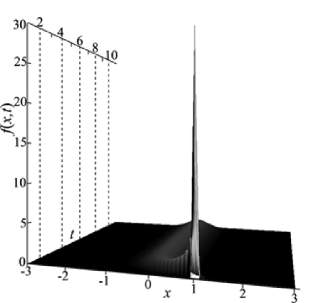
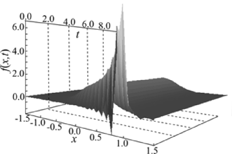
here Ex(t)=+xf(x,t)𝑑x𝐸𝑥𝑡superscriptsubscript𝑥𝑓𝑥𝑡differential-d𝑥Ex(t)={\int\limits_{-\infty}^{+\infty}{xf(x,t)}}dx is mathematical expectation, ω,θ,𝜔𝜃\omega,\,\,\,\theta, and D𝐷D are constants. With the initial spatial distribution in the form of the Dirac delta function f(x,0)=δ(xx0)𝑓𝑥0𝛿𝑥subscript𝑥0f(x,0)=\delta(x-x_{0}) the exact solution of the problem (19) takes the form (Fig.1)

f(x,t)=12πσ(t)exp[[xEx(t)]22σ(t)],𝑓𝑥𝑡12𝜋𝜎𝑡superscriptdelimited-[]𝑥𝐸𝑥𝑡22𝜎𝑡f(x,t)={\frac{{1}}{{\sqrt{2\pi\sigma(t)}}}}\exp{\left[{-{\frac{{[x-Ex(t)]^{2}}}{{2\sigma(t)}}}}\right]}, (20)

where Ex(t)=x0e(ω+θ)t,σ(t)=Dω(1e2ωt).formulae-sequence𝐸𝑥𝑡subscript𝑥0superscript𝑒𝜔𝜃𝑡𝜎𝑡𝐷𝜔1superscript𝑒2𝜔𝑡Ex(t)=x_{0}e^{-(\omega+\theta)t},\,\,\,\sigma(t)={\frac{{D}}{{\omega}}}(1-e^{-2\omega t}).

Refer to caption
Figure 1: Analytical solution (20) for the problem (19). Hereafter the parameters ω=1𝜔1\omega=1, θ=1𝜃1\theta=1, D=0.1𝐷0.1D=0.1, x0=1subscript𝑥01x_{0}=1 are chosen for the problem (19).

The accuracy and reliability of the scheme (18) was determined by the relative error

ε(t)=(Ex2(t)[Ex(t)]2)|Numσ(t)1.𝜀𝑡evaluated-at𝐸superscript𝑥2𝑡superscriptdelimited-[]𝐸𝑥𝑡2𝑁𝑢𝑚𝜎𝑡1\varepsilon(t)={\frac{{{\left.{\left({Ex^{2}(t)-[Ex(t)]^{2}}\right)}\right|}_{Num}}}{{\sigma(t)}}}-1. (21)

The expression (Ex2(t)[Ex(t)]2)|Numevaluated-at𝐸superscript𝑥2𝑡superscriptdelimited-[]𝐸𝑥𝑡2𝑁𝑢𝑚{\left.{\left({Ex^{2}(t)-[Ex(t)]^{2}}\right)}\right|}_{Num} is the second moment obtained in solving (19) by various numerical methods. Additional control was accomplished by checking the fulfillment of the condition of probability density normalization per unit l(t)=+f(x,t)𝑑xl𝑡superscriptsubscript𝑓𝑥𝑡differential-d𝑥{\rm l}(t)={\int\limits_{-\infty}^{+\infty}{f(x,t)}}dx at each time step. The condition was also used as the criterion of the correct choice of the integration region size governing the observation of boundary conditions (14).

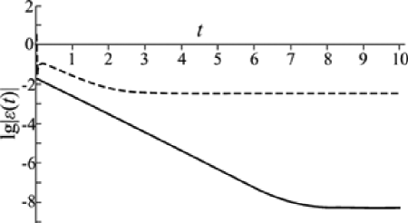
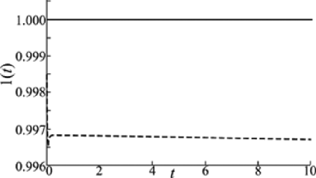
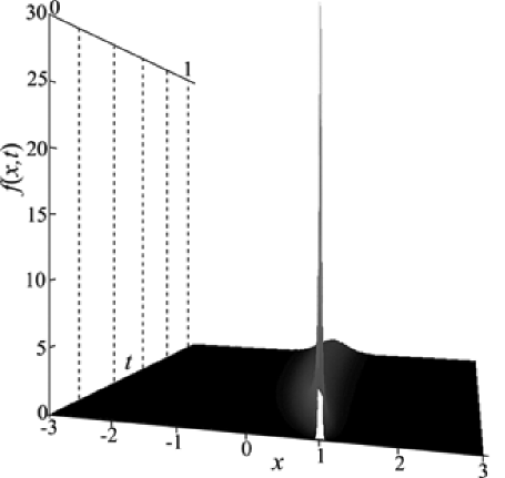
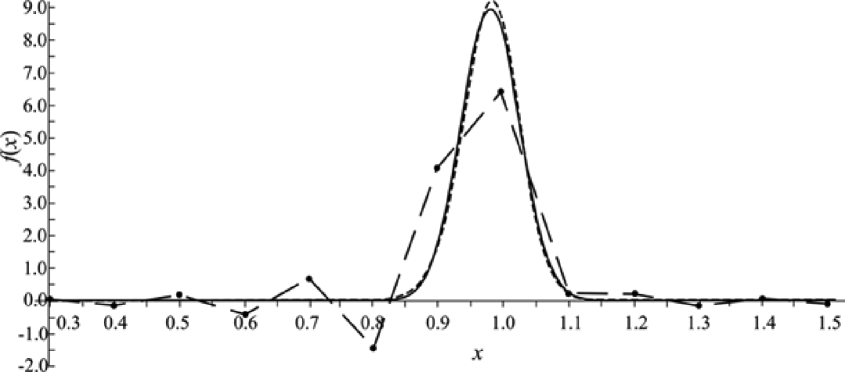
Figs. 2, 3 compare the plots of the decimal logarithm of the relative error lg|ε(t)|lg𝜀𝑡\lg|\varepsilon(t)| and probability normalization l(t)l𝑡{\rm l}(t). Fig.4 and Fig.5 demonstrate numerical solutions of eq. (19) obtained on the basis of the scheme (18) and the method based on DAF. Fig.6 shows the dependencies f(x)𝑓𝑥f(x) for t𝑡t = 0.01 for the analytical solution and the solutions obtained by methods (18) and DAF. The appropriate dependencies are obtained for the recommended (giving the least error) in Zhan11 parameters of the DAF-based method in the proper order of time approximation (O(τ))O(\tau)), the same as in scheme (18). The solution by the scheme (18) is obtained for h1=τ=0.001subscript1𝜏0.001h_{1}=\tau=0.001.

Refer to caption
Figure 2: Dependencies of the decimal algorithm of the relative error lg|ε(t)|lg𝜀𝑡\lg|\varepsilon(t)| (21) on time. The dashed line is the DAF-based method Zhan11 , the solid line is the finite-difference method (18).
Refer to caption
Figure 3: Dependencies of probability density normalization l(t)l𝑡{\rm l}(t) on time. The dashed line is the DAF-based method, the solid line is the finite-difference method (18).
Refer to caption
Figure 4: Surface f(x,t)𝑓𝑥𝑡f(x,t) obtained as a result of the numerical solution (19) by the method (18).
Refer to caption
Figure 5: Surface f(x,t)𝑓𝑥𝑡f(x,t) obtained as a result of the numerical solution (19) by the DAF-based method.
Refer to caption
Figure 6: The dependence of probability density f(x)𝑓𝑥f(x) at t=0.01𝑡0.01t=0.01. The solid line is the analytical solution (20), the dashed line is the solution obtained by method (18), and the line with a long dash is the DAF–based method Zhan11 .

It can be seen from the plots presented in Fig. 2 that in the first order of approximation over time the accuracy of the solution obtained by using scheme (18) is higher, especially when steady-state values are reached and time moments are close to the initial one. Fig. 3 shows that the dependence l(t)l𝑡{\rm l}(t) obtained by the DAF-based method is slowly decreasing, which means the violation of the normalization condition. On the contrary, scheme (18) conserves asymptotically (at large times) the condition of normalization of probability density per unit.

The analysis of Figs. 1, 4, 5, and 6 shows that scheme (18) provides the positive definiteness of probability density values at time moments close to the initial one, where the solution is close to discontinuity.

The second problem chosen for the examination of scheme (18)

f(x,t)t={[x3+(θ1)xθE(x(t))]f(x,t)}x+D2f(x,t)x2𝑓𝑥𝑡𝑡delimited-[]superscript𝑥3𝜃1𝑥𝜃𝐸𝑥𝑡𝑓𝑥𝑡𝑥𝐷superscript2𝑓𝑥𝑡superscript𝑥2{\frac{{\partial f(x,t)}}{{\partial t}}}={\frac{{\partial\{[x^{3}+(\theta-1)x-\theta E(x(t))]f(x,t)\}}}{{\partial x}}}+D{\frac{{\partial^{2}f(x,t)}}{{\partial x^{2}}}} (22)

has a larger computational complexity than problem (19), since long-lived bimodality is observed here at certain parameters, and consequently calculations are to be performed for large times. It imposes an additional requirement - asymptotic stability - on the numerical method.

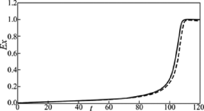
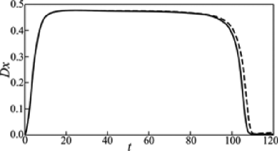
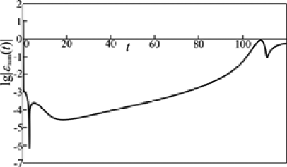
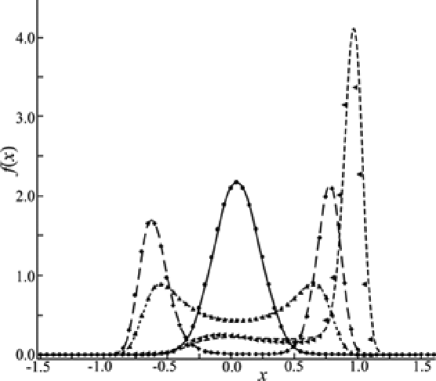
The problem (22) was solved numerically in Ref. Zhan11 by Hermite distributed approximating functional method. Below the distributions f(x)𝑓𝑥f(x) at different time moments, the dependencies of normalization 1(t)1𝑡1(t) on time, mean E(x(t))𝐸𝑥𝑡E(x(t)), variance Dx(t)=Ex2(t)[Ex(t)]2𝐷𝑥𝑡𝐸superscript𝑥2𝑡superscriptdelimited-[]𝐸𝑥𝑡2Dx(t)=Ex^{2}(t)-[Ex(t)]^{2}, and the decimal logarithm of relative error lg|εnum(t)|=Dx(t)|Eq.18Dx(t)|DAF1lgsubscript𝜀𝑛𝑢𝑚𝑡evaluated-at𝐷𝑥𝑡𝐸𝑞.18evaluated-at𝐷𝑥𝑡𝐷𝐴𝐹1\lg|\varepsilon_{num}(t)|={\frac{{Dx(t)|_{Eq.18}}}{{Dx(t)|_{DAF}}}}-1 are presented in Figs. 7-11 for comparison. In the last expression Dx(t)|Eq.18evaluated-at𝐷𝑥𝑡𝐸𝑞.18Dx(t)|_{Eq.18} is the variance calculated on the basis of scheme (18), Dx(t)|DAFevaluated-at𝐷𝑥𝑡𝐷𝐴𝐹Dx(t)|_{DAF} is the variance calculated on the basis of the DAF-based method. Here the DAF-based method solution is chosen as a benchmark for comparison.
Refer to caption
Figure 7: Distributions f(x)𝑓𝑥f(x) at time moments t𝑡t = 1, 4, 72, 105.5 obtained on the basis of scheme (18) (lines) and on the basis of the DAF-method (separate symbols). t𝑡t=1: solid line, circles; t𝑡t=4: dotted line, triangles; t𝑡t=72: line with long dash, squares; t𝑡t=105.5: dashed line, rotated triangles. Hereinafter, the parameters θ=0.5𝜃0.5\theta=0.5, D=0.01𝐷0.01D=0.01, x0=104subscript𝑥0superscript104x_{0}=10^{-4} are chosen for the problem (22).
Refer to caption
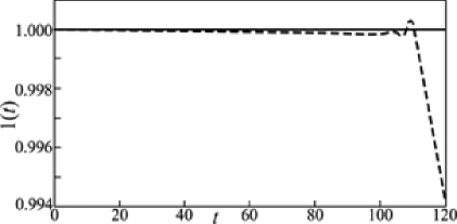
Figure 8: Dependencies of normalization l(t)l𝑡{\rm l}(t) on time for the problem (22). The dashed line is the DAF-based method Zhan11 , the solid line is the finite-difference method (18).
Refer to caption
Figure 9: Expectation Ex(t)𝐸𝑥𝑡Ex(t) vs time. The dashed line is the DAF-based method Zhan11 , the solid line is the finite-difference method (18).
Refer to caption
Figure 10: Variance Dx(t)𝐷𝑥𝑡Dx(t) vs time. The dashed line is the DAF-based method Zhan11 , the solid line is the finite-difference method (18).
Refer to caption
Figure 11: Decimal logarithm of relative error lg|εnum(t)|lgsubscript𝜀𝑛𝑢𝑚𝑡\lg|\varepsilon_{num}(t)| vs time for the problem (22).

It can be seen from Fig. 7 that the difference between numerical solutions begins to appear at times of the order of 105.5. Fig.8 gives the explanation for this. It follows from it that significant violation of the normalization condition arises at the same time. Evidently, insignificant differences in dependencies of means Ex(t)𝐸𝑥𝑡Ex(t) and variances Dx(t)𝐷𝑥𝑡Dx(t) (see Figs. 9,10) and the increase of relative error (see Fig. 11) are associated with it.

Thus, the DAF-based method limitations connected with the violation of probability density normalization condition manifest themselves stronger in the problems with large computational complexity. That is why its stability and the reliability of solution fail at large times. Also this method violates locally the positive definiteness of solutions required for the fulfillment of the standard properties of the probability density. It should be mentioned that for problem (13)-(15) functions kα(x)subscript𝑘𝛼𝑥k_{\alpha}(x) can have a complicated form. This would entail the expansion of the integration region G𝐺G to observe the boundary condition (14). For n>20𝑛20n>20 and large x𝑥x Hermite’s polynomials H2n(x)subscript𝐻2𝑛𝑥H_{2n}(x) used in the DAF-based method can acquire values that require the application of arbitrary-precision arithmetic. This leads to even greater computational complexity and also limits the application of the method.

Method (18) is free from the above features. The necessity of choosing a sufficiently dense uniform mesh can be classified as a limitation of scheme (18). However this can be avoided by choosing a mesh with a variable space step. It is possible to construct an unconditionally stable homogeneous conservative finite-difference scheme for problem (13) - (15) on a non-uniform mesh using Refs. Samar39 ; Samar40 .

IV SPATIALLY EXTENDED STOCHASTIC BRUSSELATOR

IV.1 Mean-field result

Let us apply the method developed in Sec. III to the study of probability density of the system describing the well known model of autocatalytic chemical reaction (brusselator Prig28 ) with spatially correlated multiplicative noise. Simultaneously let us study the variance of some statistical first- and second-order characteristics of the system by increasing the intensity of the external noise. In this paper the range of parameters at which the Turing bifurcation arises in a deterministic system is considered.

Brusselator is a model of a simple autocatalytic chemical reaction having a trimolecular step Prig28 . The concentrations of the initial and final products in this reaction are maintained constant. The influence of external fluctuating environment can lead to the fact that concentrations of the initial and final products become random functions. This leads to the necessity of including noise into the kinetic equations of a deterministic model. Let us assume that the concentration of the initial product Binsubscript𝐵𝑖𝑛B_{in} is most affected by external random environment. Then kinetic equations of the reaction under consideration have the form:

x1t=A+x12x2(B+1+ξ1(𝐫,t))x1+D12x1,x2t=x12x2+(B+ξ2(𝐫,t))x1+D22x2,formulae-sequencesubscript𝑥1𝑡𝐴superscriptsubscript𝑥12subscript𝑥2𝐵1subscript𝜉1𝐫𝑡subscript𝑥1subscript𝐷1superscript2subscript𝑥1subscript𝑥2𝑡superscriptsubscript𝑥12subscript𝑥2𝐵subscript𝜉2𝐫𝑡subscript𝑥1subscript𝐷2superscript2subscript𝑥2{\frac{{\partial x_{1}}}{{\partial t}}}=A+x_{1}^{2}x_{2}-(B+1+\xi_{1}(\mathbf{r},t))x_{1}+D_{1}\nabla^{2}x_{1},\\ {\frac{{\partial x_{2}}}{{\partial t}}}=-x_{1}^{2}x_{2}+(B+\xi_{2}(\mathbf{r},t))x_{1}+D_{2}\nabla^{2}x_{2}, (23)

where x1subscript𝑥1x_{1}, x2subscript𝑥2x_{2} are concentrations of intermediate components, D1subscript𝐷1D_{1}, D2subscript𝐷2D_{2} are their diffusion coefficients, A𝐴A, Binsubscript𝐵𝑖𝑛B_{in} are concentrations of initial products with Bin=B+ξi(𝐫,t)subscript𝐵𝑖𝑛𝐵subscript𝜉𝑖𝐫𝑡B_{in}=B+\xi_{i}(\mathbf{r},t). Parameter B𝐵B is the spatio-temporal average of the initial product concentration Binsubscript𝐵𝑖𝑛B_{in}. The decrease in concentration x1subscript𝑥1x_{1} is due to the two decays: with the formation of one of the final products and with the formation of an intermediate product x2subscript𝑥2x_{2} and the second final product. These decays have different chemical reaction rates which are affected by external noises in different ways. It is taken into account by including different uncorrelated fields ξi(𝐫,t)subscript𝜉𝑖𝐫𝑡\xi_{i}(\mathbf{r},t) into Eqs. (23). Statistical properties of the fields ξi(𝐫,t)subscript𝜉𝑖𝐫𝑡\xi_{i}(\mathbf{r},t) are described in Sec. I.

The system of equations (23) is a specific case of Eq. (1) with n𝑛n = 2. Therefore, multidimensional single-site NSCFPE in the Stratonovitch interpretation can be immediately written for the model (23) using Eq. (12):

w(x1,x2,t)t=x1{[Ax12x2+(B+1+θ1)x1D1(E(x1|x2)x1)]w+θ1Φ1,0x12wx1}+𝑤subscript𝑥1subscript𝑥2𝑡𝑡limit-fromsubscript𝑥1delimited-[]𝐴superscriptsubscript𝑥12subscript𝑥2𝐵1subscript𝜃1subscript𝑥1subscript𝐷1𝐸conditionalsubscript𝑥1subscript𝑥2subscript𝑥1𝑤subscript𝜃1subscriptΦ10superscriptsubscript𝑥12𝑤subscript𝑥1{\frac{{\partial w(x_{1},x_{2},t)}}{{\partial t}}}={\frac{{\partial}}{{\partial x_{1}}}}{\left\{{{\left[{-A-x_{1}^{2}x_{2}+(B+1+\theta_{1})x_{1}-D_{1}(E(x_{1}|x_{2})-x_{1})}\right]}w+\theta_{1}\Phi_{1,0}x_{1}^{2}{\frac{{\partial w}}{{\partial x_{1}}}}}\right\}}+
x2{[x12x2Bx1D2(E(x2|x1)x2)]w+θ2Φ2,0x12wx2},subscript𝑥2delimited-[]superscriptsubscript𝑥12subscript𝑥2𝐵subscript𝑥1subscript𝐷2𝐸conditionalsubscript𝑥2subscript𝑥1subscript𝑥2𝑤subscript𝜃2subscriptΦ20superscriptsubscript𝑥12𝑤subscript𝑥2{\frac{{\partial}}{{\partial x_{2}}}}{\left\{{{\left[{x_{1}^{2}x_{2}-Bx_{1}-D_{2}(E(x_{2}|x_{1})-x_{2})}\right]}w+\theta_{2}\Phi_{2,0}x_{1}^{2}{\frac{{\partial w}}{{\partial x_{2}}}}}\right\}}, (24)
E(x1|x2,t)=+x1w(x1|x2,t)𝑑x1,E(x2|x1,t)=+x2w(x2|x1,t)𝑑x2,formulae-sequence𝐸conditionalsubscript𝑥1subscript𝑥2𝑡superscriptsubscriptsubscript𝑥1𝑤conditionalsubscript𝑥1subscript𝑥2𝑡differential-dsubscript𝑥1𝐸conditionalsubscript𝑥2subscript𝑥1𝑡superscriptsubscriptsubscript𝑥2𝑤conditionalsubscript𝑥2subscript𝑥1𝑡differential-dsubscript𝑥2E(x_{1}|x_{2},t)={\int\limits_{-\infty}^{+\infty}{x_{1}w(x_{1}|x_{2},t)dx_{1}}},\quad E(x_{2}|x_{1},t)={\int\limits_{-\infty}^{+\infty}{x_{2}w(x_{2}|x_{1},t)dx_{2}}},
w(x1|x2,t)=w(x1,x2,t)+w(x1,x2,t)𝑑x1,w(x2|x1,t)=w(x1,x2,t)+w(x1,x2,t)𝑑x2.formulae-sequence𝑤conditionalsubscript𝑥1subscript𝑥2𝑡𝑤subscript𝑥1subscript𝑥2𝑡superscriptsubscript𝑤subscript𝑥1subscript𝑥2𝑡differential-dsubscript𝑥1𝑤conditionalsubscript𝑥2subscript𝑥1𝑡𝑤subscript𝑥1subscript𝑥2𝑡superscriptsubscript𝑤subscript𝑥1subscript𝑥2𝑡differential-dsubscript𝑥2w(x_{1}|x_{2},t)={\frac{{w(x_{1},x_{2},t)}}{{{\int\limits_{-\infty}^{+\infty}{w(x_{1},x_{2},t)dx_{1}}}}}},\quad w(x_{2}|x_{1},t)={\frac{{w(x_{1},x_{2},t)}}{{{\int\limits_{-\infty}^{+\infty}{w(x_{1},x_{2},t)dx_{2}}}}}}.

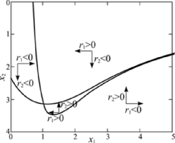
Numerical solutions for Eq. (24) are obtained using the finite-difference scheme (18) (see Appendix A). Eq. (24) has a greater computational complexity than, for example, the problems (19) and (22). This is related to the fact that, first, the drift coefficients r1,2(x1,x2,t)subscript𝑟12subscript𝑥1subscript𝑥2𝑡r_{1,2}(x_{1},x_{2},t) are nonlinear and alternating-sign. This leads to the fact that regions with the different direction of the probability density drift arise on the plane (x1,x2)subscript𝑥1subscript𝑥2\left({x_{1},x_{2}}\right) (see Fig. 12). Moreover, the boundaries of these regions defined by the equations r1,2(x1,x2,t)=0subscript𝑟12subscript𝑥1subscript𝑥2𝑡0r_{1,2}(x_{1},x_{2},t)=0 are moving since conditional means E(x1|x2,t),E(x2|x1,t)𝐸conditionalsubscript𝑥1subscript𝑥2𝑡𝐸conditionalsubscript𝑥2subscript𝑥1𝑡E(x_{1}|x_{2},t),E(x_{2}|x_{1},t) are time functions. Second, the diffusion coefficients are proportional to x12superscriptsubscript𝑥12x_{1}^{2}, which leads to a significant increase of the integration region necessary to satisfy the boundary conditions (14). Third, the problem (24) is two-dimensional and increasing the dimension of the space always leads to an increase of computational complexity.
Refer to caption
Figure 12: Probability density (24) drift directions on the plane (x1,x2)subscript𝑥1subscript𝑥2\left({x_{1},x_{2}}\right). Parameters are A𝐴A=3, B𝐵B=7, θ1=θ2=0.1subscript𝜃1subscript𝜃20.1\theta_{1}=\theta_{2}=0.1, D1subscript𝐷1D_{1}=1, D2subscript𝐷2D_{2}=5, E(x1|x2,t)=A,E(x2|x1,t)=B/Aformulae-sequence𝐸conditionalsubscript𝑥1subscript𝑥2𝑡𝐴𝐸conditionalsubscript𝑥2subscript𝑥1𝑡𝐵𝐴E(x_{1}|x_{2},t)=A,E(x_{2}|x_{1},t)=B/A, Φ1,0=Φ2,0=1subscriptΦ10subscriptΦ201\Phi_{1,0}=\Phi_{2,0}=1.

Figures 13, 17, 21, 22 present characteristic types of solutions (24) obtained at different values of the parameters of the problem and the noise intensity. The initial distribution is Gaussian with variances θ1subscript𝜃1\theta_{1} and θ2subscript𝜃2\theta_{2}, and expectations equal to stationary values of x10subscript𝑥10x_{10} and x20subscript𝑥20x_{20} in the absence of noise (see Appendix A). The following parameters for numerical integration (24) remain constant in our calculations: A𝐴A=3, D1=1subscript𝐷11D_{1}=1, D2=5subscript𝐷25D_{2}=5, Φ1,0=Φ2,0=1subscriptΦ10subscriptΦ201\Phi_{1,0}=\Phi_{2,0}=1. The other parameters are indicated under the figures. The critical value of parameter B𝐵B is 5.47 in a deterministic case at given A𝐴A, D1subscript𝐷1D_{1}, and D2subscript𝐷2D_{2}.

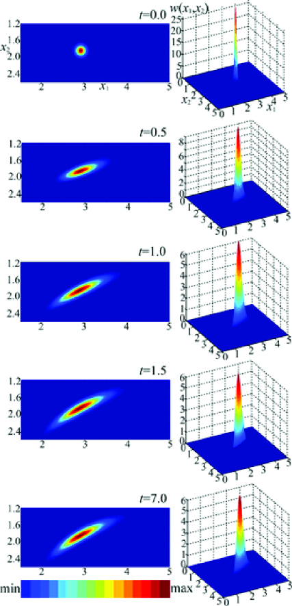
Fig. 13 demonstrates the evolution of probability density w(x1,x2,t)𝑤subscript𝑥1subscript𝑥2𝑡w(x_{1},x_{2},t) in the vicinity of the deterministic bifurcation point and small noise intensity. It can be seen from this figure that the symmetry of initial distribution is violated in the evolution process. The probability density distribution remains unimodal throughout the time until the stationary state is reached. Hence the state of the system (23) is ordered, despite the noise.
Refer to caption
Figure 13: The evolution of probability density (24) for the model (23). Unimodal distribution (top view in the left-hand side). The color gradient from dark blue to dark red visualizes the change from minimum to maximum. The model parameters are B𝐵B=5.5, θ1=θ2=0.005subscript𝜃1subscript𝜃20.005\theta_{1}=\theta_{2}=0.005. The time moment t𝑡t=7 corresponds to the stationary state.
Refer to caption

a)
Refer to caption
b)

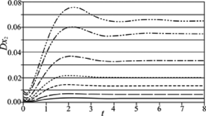
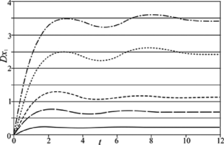
Figure 14: The dependencies of variance Dx𝐷𝑥Dx of concentration on time with increasing noise intensity: a) first product, b) second product. The solid line θ1=θ2=θ=0.0005subscript𝜃1subscript𝜃2𝜃0.0005\theta_{1}=\theta_{2}=\theta=0.0005, the line with a long dash θ=0.001𝜃0.001\theta=0.001, the dashed line θ=0.002𝜃0.002\theta=0.002, the dotted line θ=0.003𝜃0.003\theta=0.003, the dash-dotted line θ=0.005𝜃0.005\theta=0.005, the dash-dot-dot line θ=0.008𝜃0.008\theta=0.008, the three dots - dash line θ=0.01𝜃0.01\theta=0.01. B𝐵B=5.5
Refer to caption

a)
Refer to caption
b)

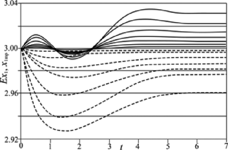
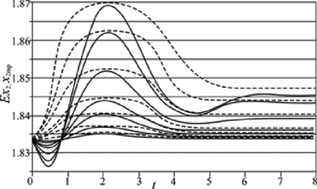
Figure 15: Fig. 15. The dependencies of mean Ex𝐸𝑥Ex (solid lines) and most probable xmpsubscript𝑥mpx_{\rm{mp}} (dashed lines) values on time in case of increasing noise intensity: a) first product, b) second product. B𝐵B=5.5. θ1,θ2subscript𝜃1subscript𝜃2\theta_{1},\theta_{2} are as in Fig. 14. The greater the noise intensity, the greater the deviation of values Ex𝐸𝑥Ex and xmpsubscript𝑥mpx_{\rm{mp}} from the stationary values of x10subscript𝑥10x_{10} and x20subscript𝑥20x_{20} (t𝑡t=0).
Refer to caption
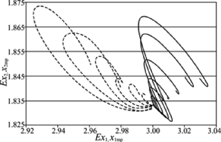
Figure 16: Changes of the mean Ex𝐸𝑥Ex (solid lines) and most probable xmpsubscript𝑥mpx_{\rm{mp}} (dashed lines) values x1subscript𝑥1x_{1} and x2subscript𝑥2x_{2} in case of increasing noise intensity for unimodal distribution. B𝐵B=5.5. θ1,θ2subscript𝜃1subscript𝜃2\theta_{1},\theta_{2} are as in Fig. 14. The greater the noise intensity, the greater the size of the wreath of the curve.

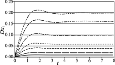
Fig. 14 shows the appropriate dependencies of variance of concentrations x1subscript𝑥1x_{1} and x2subscript𝑥2x_{2} on time if noise intensity increases. It can be seen that the greater external noise intensity, the faster the variance increases and the greater its value in the stationary state. Fig. 15 demonstrates the dependencies of the mean and most probable values on time with different noise intensities. The increase of noise intensity leads to the increase of difference between the mean and the appropriate most probable in the steady stationary state. Fig. 16 illustrates this more clearly. All the results given above are quite expectable.

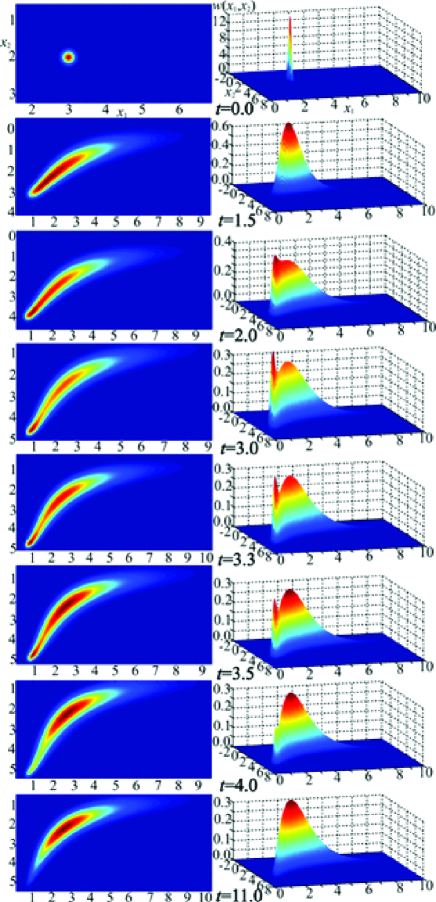
Quite a different picture is observed at a greater distance from the deterministic bifurcation point. Fig. 17 presents a more complicated type of the probability density w(x1,x2,t)𝑤subscript𝑥1subscript𝑥2𝑡w(x_{1},x_{2},t) evolution. We can see that at first unimodal distribution is conserved, but it is strongly ”blurred” and the maximum of density drifts away from the initial position. Then the splitting of probability density with the formation of two maxima takes place at a certain point in time. Bimodal probability distribution ”lives” during a certain time interval. Herewith competition occurs between maxima, as a result of which one of the maxima suppresses the other. The distribution becomes unimodal again. That is, transient bimodality is observed in the ordered phase. The behavior of the statistical characteristics also varies as the noise intensity increases.

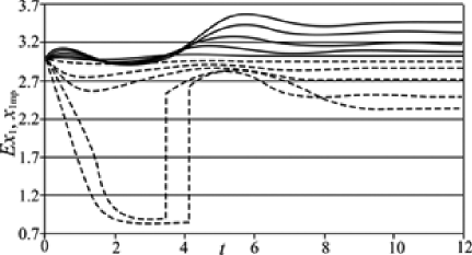
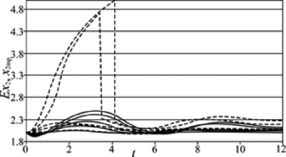
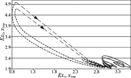
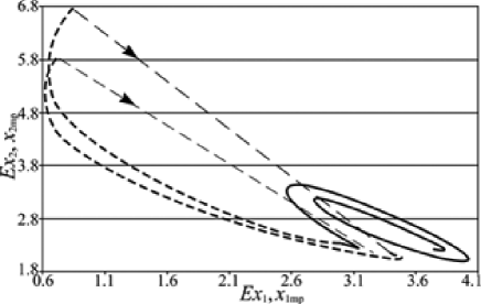
Fig. 18 shows the dependencies of variance Dx1𝐷subscript𝑥1Dx_{1} of concentration of the first product on time when the noise intensity increases. Figs. 19, 20 demonstrate the appropriate changes of the mean and most probable values. Dependencies Dx1(t)𝐷subscript𝑥1𝑡Dx_{1}(t), Exi(t),ximp(t)𝐸subscript𝑥𝑖𝑡subscript𝑥𝑖mp𝑡Ex_{i}(t),x_{i{\rm mp}}(t) are similar to the ones given in Figs. 14,15,16 if the noise intensities θ1,θ2<0.09subscript𝜃1subscript𝜃20.09\theta_{1},\theta_{2}<0.09. The distribution remains unimodal. A clearly visible ”dip” corresponding to the disappearance of transient bimodality is observed in the dependence Dx1(t)𝐷subscript𝑥1𝑡Dx_{1}(t) at θ1,θ20.09subscript𝜃1subscript𝜃20.09\theta_{1},\theta_{2}\geq 0.09. Herewith the discontinuity of the first kind appears in plots of the most probable vs time. The jump from a wreath of the curve x2mp(x1mp)subscript𝑥2mpsubscript𝑥1mpx_{2{\rm mp}}(x_{1{\rm mp}}) corresponds to the disappearance of transient bimodality in Fig. 20.
Refer to caption
Figure 17: The evolution of probability density (24) for the model (23). Transient bimodality is observed in the time interval t[1.5,4]𝑡1.54t\in[1.5,4]. Model parameters are B𝐵B=6, θ1=θ2=0.09subscript𝜃1subscript𝜃20.09\theta_{1}=\theta_{2}=0.09. The time moment t𝑡t=11 corresponds to the setting of the stationary state.
Refer to caption
Figure 18: Dependencies of variance Dx1𝐷subscript𝑥1Dx_{1} of concentration x1subscript𝑥1x_{1} on time with increasing noise intensity. The solid line θ1=θ2=θ=0.01subscript𝜃1subscript𝜃2𝜃0.01\theta_{1}=\theta_{2}=\theta=0.01, the line with a long dash θ=0.03𝜃0.03\theta=0.03, the dashed line θ=0.05𝜃0.05\theta=0.05, the dotted line θ=0.09𝜃0.09\theta=0.09, the dash-dotted line θ=0.12𝜃0.12\theta=0.12. B𝐵B=6.
Refer to caption

a)
Refer to caption
b)

Figure 19: The dependencies of mean Ex𝐸𝑥Ex (solid lines) and most probable xmpsubscript𝑥mpx_{\rm{mp}} (dashed lines) values on time with increasing noise intensity: a) first product, b) second product. B𝐵B=6. θ1,θ2subscript𝜃1subscript𝜃2\theta_{1},\theta_{2} are as in Fig. 14. The greater the noise intensity, the greater the deviation of values Ex𝐸𝑥Ex and xmpsubscript𝑥mpx_{\rm{mp}} from the stationary values of x10subscript𝑥10x_{10} and x20subscript𝑥20x_{20}. The most probable jump (discontinuity of the first kind) corresponds to the disappearance of bimodality.
Refer to caption
Figure 20: Changes of the mean Ex𝐸𝑥Ex (solid lines) and the most probable xmpsubscript𝑥mpx_{\rm{mp}} (dashed lines) values x1subscript𝑥1x_{1} and x2subscript𝑥2x_{2} in case of increasing the noise intensity. B𝐵B=6, the other model parameters are as in Fig. 18. A jump from a wreath of the curve x2mp(x1mp)subscript𝑥2mpsubscript𝑥1mpx_{2{\rm mp}}(x_{1{\rm mp}}) shown in the figure by a thin line with a dash and the arrow corresponds to the disappearance of bimodality.
Refer to caption
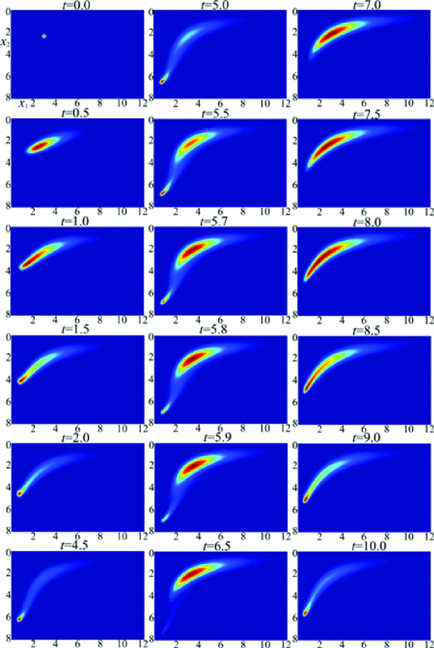
Figure 21: The evolution of probability density (24) for the model (23). ”Repumping” of probability density through bimodality (top view). The model parameters are B𝐵B=7, θ1=θ2=θ=0.1subscript𝜃1subscript𝜃2𝜃0.1\theta_{1}=\theta_{2}=\theta=0.1. The figure presents one ”period” of ”repumping”. The sequences of the frames in the left-hand side and the right-hand side correspond to unimodal distribution, while in the center they correspond to the bimodal one.
Refer to caption
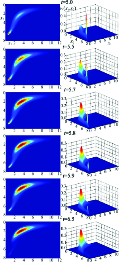
Figure 22: ”Repumping” of probability density through bimodality (corresponds to the center of Fig.21).
Refer to caption
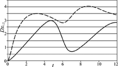
Figure 23: Dependencies of variances Dx1𝐷subscript𝑥1Dx_{1} and Dx2𝐷subscript𝑥2Dx_{2} on time at B𝐵B=7, θ1=θ2=θ=0.1subscript𝜃1subscript𝜃2𝜃0.1\theta_{1}=\theta_{2}=\theta=0.1. The figure presents one ”period of repumping”.
Refer to caption
Figure 24: Change of the mean (solid line) and the most probable (dashed line) values x1subscript𝑥1x_{1} and x2subscript𝑥2x_{2} in ”repumping”. Two ”periods” are presented.

A completely unexpected solution (24) appears at a greater distance from the deterministic point of bifurcation (see Figs. 21-24). At first density drifts from the initial position to the boundary of the integration region in accordance with the directions indicated in Fig. 12. Then the splitting of density occurs at tsimilar-to𝑡absentt\sim5 (Figs. 21, 22) just as in transient bimodality.

Peculiar ”repumping” of probability density from one maximum to another through bimodality is observed until the time moment tsimilar-to𝑡absentt\sim6.5 (Fig. 22). It can be noticed that the duration of the existence of one- and bimodal distributions are comparable in the order of magnitude. Then a drift towards the boundaries happens again. The process is repeated until the stationary state is established. This is accompanied by a gradual decrease of maximum values in Dxi(t)𝐷subscript𝑥𝑖𝑡Dx_{i}(t) (Fig. 23), and decrease in the size of the wreath of the curve Ex2(Ex1)𝐸subscript𝑥2𝐸subscript𝑥1Ex_{2}(Ex_{1}) (Fig. 24). Figure 24 shows two jumps from a wreath of the curve x2mp(x1mp)subscript𝑥2mpsubscript𝑥1mpx_{2\rm{mp}}(x_{1\rm{mp}}), which corresponds to the double appearance and disappearance of ”repumping” of the probability density through bimodality.

Such behavior of the probability density implies multiple appearance of the other state (other phase) that corresponds to bimodal distribution, in the ordered phase. We can assume that there is a kind of phase ”intermittency”. This noise-induced effect will be presented in more detail in our future paper.

So, as a result of the numerical study of Eq. (24) solutions we found that different type of solutions can arise in the region of Turing bifurcation when noise intensity increases: unimodal distribution, unimodal distribution with transient bimodality, and complicated distribution, in which unimodal and bimodal distributions alternate until the steady state is established. In other words, only the ordered phase is observed at low noise intensity. The increase of the noise intensity leads to the appearance of transient bimodality (disordered phase) in the ordered phase. Further growth of the noise intensity disrupts the ordering to an even greater extent: there is an ”intermittency” phase, which ”swings” the ordered state, as it were.

IV.2 Fokker-Planck equation for order parameters

The system (23) analysis presented above takes into account the interaction of the whole set of both stable and unstable modes. It is known that the system behavior is governed by the behavior of unstable modes (order parameters) Haken41 in the vicinity of the Turing bifurcation point. Therefore, additionally we study the behavior of order parameters of this system. The procedure of deriving generalized Ginzburg - Landau equations for type (1) systems was proposed in Ref. Kur27 . Following this procedure we obtained stochastic equations for the amplitudes of unstable modes for system (23). These equations have the form:

dξ𝐤u(1)dτ=F𝐤u(τ),𝑑superscriptsubscript𝜉𝐤𝑢1𝑑𝜏subscript𝐹𝐤𝑢𝜏{\frac{{d\xi_{\mathbf{k}u}^{(1)}}}{{d\tau}}}=F_{\mathbf{k}u}(\tau), (25)
F𝐤u(τ)=λ1(𝐤u)ξ𝐤u(1)+𝐤uΩ1(𝐤u,𝐤u,𝐤s,𝐳(τ))ξ𝐤u(1)+subscript𝐹𝐤𝑢𝜏subscript𝜆1subscript𝐤𝑢superscriptsubscript𝜉𝐤𝑢1limit-fromsubscriptsuperscript𝐤𝑢subscriptΩ1subscript𝐤𝑢subscriptsuperscript𝐤𝑢subscript𝐤𝑠𝐳𝜏superscriptsubscript𝜉superscript𝐤𝑢1F_{\mathbf{k}u}(\tau)=\lambda_{1}({\mathbf{k}}_{u})\xi_{\mathbf{k}u}^{(1)}+{\sum\limits_{{\mathbf{k}}^{\prime}u}{\Omega_{1}({\mathbf{k}}_{u},{\mathbf{k}^{\prime}}_{u},{\mathbf{k}}_{s},{\mathbf{z}}(\tau))\xi_{{\mathbf{k}}^{\prime}u}^{(1)}}}+
𝐤u𝐤′′uΩ11(𝐤u,𝐤u,𝐤′′u,𝐤s,𝐳(τ))ξ𝐤u(1)ξ𝐤′′u(1)+𝐤u𝐤′′u𝐤′′′uω(𝐤u,𝐤u,𝐤′′u,𝐤′′′u)ξ𝐤u(1)ξ𝐤′′u(1)ξ𝐤′′′u(1)+subscriptsuperscript𝐤𝑢superscript𝐤′′𝑢subscriptΩ11subscript𝐤𝑢subscriptsuperscript𝐤𝑢subscriptsuperscript𝐤′′𝑢subscript𝐤𝑠𝐳𝜏superscriptsubscript𝜉superscript𝐤𝑢1superscriptsubscript𝜉superscript𝐤′′𝑢1limit-fromsubscriptsuperscript𝐤𝑢superscript𝐤′′𝑢superscript𝐤′′′𝑢𝜔subscript𝐤𝑢subscriptsuperscript𝐤𝑢subscriptsuperscript𝐤′′𝑢subscriptsuperscript𝐤′′′𝑢superscriptsubscript𝜉superscript𝐤𝑢1superscriptsubscript𝜉superscript𝐤′′𝑢1superscriptsubscript𝜉superscript𝐤′′′𝑢1{\sum\limits_{{\mathbf{k}}^{\prime}u{\mathbf{k}}^{\prime\prime}u}{\Omega_{11}({\mathbf{k}}_{u},{\mathbf{k}^{\prime}}_{u},{\mathbf{k}^{\prime\prime}}_{u},{\mathbf{k}}_{s},{\mathbf{z}}(\tau))}}\xi_{{\mathbf{k}}^{\prime}u}^{(1)}\xi_{{\mathbf{k}}^{\prime\prime}u}^{(1)}+{\sum\limits_{{\mathbf{k}}^{\prime}u{\mathbf{k}}^{\prime\prime}u{\mathbf{k}}^{\prime\prime\prime}u}{\omega({\mathbf{k}}_{u},{\mathbf{k}^{\prime}}_{u},{\mathbf{k}^{\prime\prime}}_{u},{\mathbf{k}^{\prime\prime\prime}}_{u})}}\xi_{{\mathbf{k}}^{\prime}u}^{(1)}\xi_{{\mathbf{k}}^{\prime\prime}u}^{(1)}\xi_{{\mathbf{k}}^{\prime\prime\prime}u}^{(1)}+
A[O1(1)(𝐤u)z1,𝐤u(τ)+O2(1)(𝐤u)z2,𝐤u(τ)]μ,φ,φ=12𝐤sζφφ(μ)(𝐤s,𝐤u)zφ,𝐤u𝐤s(τ)zφ,𝐤s(τ).𝐴delimited-[]superscriptsubscript𝑂1absent1subscript𝐤𝑢subscript𝑧1𝐤𝑢𝜏superscriptsubscript𝑂2absent1subscript𝐤𝑢subscript𝑧2𝐤𝑢𝜏superscriptsubscript𝜇𝜑superscript𝜑12subscript𝐤𝑠superscriptsubscript𝜁𝜑superscript𝜑𝜇subscript𝐤𝑠subscript𝐤𝑢subscript𝑧superscript𝜑𝐤𝑢𝐤𝑠𝜏subscript𝑧𝜑𝐤𝑠𝜏A{\left[{-O_{1}^{*(1)}({\mathbf{k}}_{u})z_{1,{\mathbf{k}}u}(\tau)+O_{2}^{*(1)}({\mathbf{k}}_{u})z_{2,{\mathbf{k}}u}(\tau)}\right]}-{\sum\limits_{\mu,\varphi,{\varphi}^{\prime}=1}^{2}{{\sum\limits_{{\mathbf{k}}s}{\zeta_{\varphi{\varphi}^{\prime}}^{(\mu)}({\mathbf{k}}_{s},{\mathbf{k}}_{u})z_{{\varphi}^{\prime},{\mathbf{k}}u-{\mathbf{k}}s}(\tau)}}}}z_{\varphi,{\mathbf{k}}s}(\tau).

Here ξ𝐤u(1)superscriptsubscript𝜉𝐤𝑢1\xi_{{\mathbf{k}}u}^{(1)} are unstable mode amplitudes of system (23), 𝐤u,𝐤ssubscript𝐤𝑢subscript𝐤𝑠{\mathbf{k}}_{u},{\mathbf{k}}_{s} are wave numbers of unstable and stable modes respectively, 𝐳(τ)𝐳𝜏{\mathbf{z}}(\tau) is the random vector field, the components of which zφ,𝐤(τ)=ξφ(𝐫,τ)ei𝐤𝐫𝑑𝐫subscript𝑧𝜑𝐤𝜏subscript𝜉𝜑𝐫𝜏superscript𝑒𝑖𝐤𝐫differential-d𝐫z_{\varphi,{\mathbf{k}}}(\tau)=\int{\xi_{\varphi}({\mathbf{r}},\tau)e^{-i{\mathbf{k}}{\mathbf{r}}}d{\mathbf{r}}} have zero means and a given correlation tensor K[zj,𝐤(t),zl,𝐤(τ)]=gjl(|𝐤|)δ(𝐤𝐤)δ(tτ)δjl𝐾subscript𝑧𝑗𝐤𝑡subscript𝑧𝑙superscript𝐤𝜏subscript𝑔𝑗𝑙𝐤𝛿𝐤superscript𝐤𝛿𝑡𝜏subscript𝛿𝑗𝑙K[z_{j,{\mathbf{k}}}(t),z_{l,{\mathbf{k}^{\prime}}}(\tau)]=g_{jl}({\left|{{\mathbf{k}}}\right|})\delta({\mathbf{k}}-{\mathbf{k}^{\prime}})\delta(t-\tau)\delta_{jl}, φ𝜑\varphi and 𝐤𝐤\mathbf{k} are index arguments of this field. Taking into account that the functions Φi(|𝐫𝐫|)subscriptΦ𝑖𝐫superscript𝐫\Phi_{i}({\left|{{\mathbf{r}}-{\mathbf{r}^{\prime}}}\right|}) in Eqs. (1) were chosen to be exponential for definiteness, for two-dimensional media gii=θikfi/[2π2(k2+kfi2)3/2]subscript𝑔𝑖𝑖subscript𝜃𝑖subscript𝑘𝑓𝑖delimited-[]2superscript𝜋2superscriptsuperscript𝑘2superscriptsubscript𝑘𝑓𝑖232g_{ii}=\theta_{i}k_{fi}/[2\pi^{2}(k^{2}+k_{fi}^{2})^{-3/2}]. Functions λ1(𝐤u)subscript𝜆1subscript𝐤𝑢\lambda_{1}({\mathbf{k}}_{u}), Ω1(𝐤u,𝐤u,𝐤s,𝐳(τ))subscriptΩ1subscript𝐤𝑢subscriptsuperscript𝐤𝑢subscript𝐤𝑠𝐳𝜏\Omega_{1}({\mathbf{k}}_{u},{\mathbf{k}^{\prime}}_{u},{\mathbf{k}}_{s},{\mathbf{z}}(\tau)), Ω11(𝐤u,𝐤u,𝐤′′u,𝐤s,𝐳(τ)\Omega_{11}({\mathbf{k}}_{u},{\mathbf{k}^{\prime}}_{u},{\mathbf{k}^{\prime\prime}}_{u},{\mathbf{k}}_{s},{\mathbf{z}}(\tau) and others introduced in Eq. (25) are presented in Appendix B.

Equations (25) define the evolution of a set of random processes. Let us write FPE for these processes. It can be represented in a general form as follows:

w({ξ𝐤u(1)},τ)τ=𝐤uξ𝐤u(1){(<F𝐤u(τ)>+𝐪u0K[F𝐤u(τ)ξ𝐪u(1),F𝐪u(t)]𝑑t)w}+𝑤superscriptsubscript𝜉𝐤𝑢1𝜏𝜏limit-fromsubscript𝐤𝑢superscriptsubscript𝜉𝐤𝑢1expectationsubscript𝐹𝐤𝑢𝜏subscript𝐪𝑢superscriptsubscript0𝐾subscript𝐹𝐤𝑢𝜏superscriptsubscript𝜉𝐪𝑢1subscript𝐹𝐪𝑢superscript𝑡differential-dsuperscript𝑡𝑤{\frac{{\partial w\left({{\left\{{\xi_{{\mathbf{k}}u}^{(1)}}\right\}},\tau}\right)}}{{\partial\tau}}}=-{\sum\limits_{{\mathbf{k}}u}{{\frac{{\partial}}{{\partial\xi_{{\mathbf{k}}u}^{(1)}}}}{\left\{{\left({<F_{{\mathbf{k}}u}(\tau)>+{\sum\limits_{{\mathbf{q}}u}{{\int\limits_{-\infty}^{0}{K[{\frac{{\partial F_{{\mathbf{k}}u}(\tau)}}{{\partial\xi_{{\mathbf{q}}u}^{(1)}}}},F_{{\mathbf{q}}u}({t}^{\prime})]}}}}d{t}^{\prime}}\right)w}\right\}}}}+ (26)
+𝐤u,𝐪u2ξ𝐤u(1)ξ𝐪u(1){(0K[F𝐤u(τ),F𝐪u(t)]𝑑t)w}.subscript𝐤𝑢𝐪𝑢superscript2superscriptsubscript𝜉𝐤𝑢1superscriptsubscript𝜉𝐪𝑢1superscriptsubscript0𝐾subscript𝐹𝐤𝑢𝜏subscript𝐹𝐪𝑢superscript𝑡differential-dsuperscript𝑡𝑤+{\sum\limits_{{\mathbf{k}}u,{\mathbf{q}}u}{{\frac{{\partial^{2}}}{{\partial\xi_{{\mathbf{k}}u}^{(1)}\partial\xi_{{\mathbf{q}}u}^{(1)}}}}{\left\{{\left({{\int\limits_{-\infty}^{0}{K[F_{{\mathbf{k}}u}(\tau),F_{{\mathbf{q}}u}({t}^{\prime})]}}d{t}^{\prime}}\right)w}\right\}}}}.

Here w({ξ𝐤u(1)},τ)𝑤superscriptsubscript𝜉𝐤𝑢1𝜏w\left({{\left\{{\xi_{{\mathbf{k}}u}^{(1)}}\right\}},\tau}\right) is the multivariate probability distribution density defining the probability of some configuration of unstable modes {ξ𝐤u(1)}superscriptsubscript𝜉𝐤𝑢1{\left\{{\xi_{{\mathbf{k}}u}^{(1)}}\right\}} . After transformations with an accuracy up to the terms linear in the noise intensity one can obtain the correlation functions appearing in Eq. (26) that are presented in Appendix C.

Let the space of the system under study be two-dimensional. If only one mode with the wave number 𝐤csubscript𝐤𝑐{\mathbf{k}}_{c} and amplitude ξ𝐤csubscript𝜉𝐤𝑐\xi_{{\mathbf{k}}c} is unstable in such space the Eq. (26) acquires a simple structure:

w(ξ𝐤c,τ)τ=ξ𝐤c{(h+aξ𝐤c+bξ𝐤c3)w(c+dξ𝐤c2+eξ𝐤c4)wξ𝐤c}.𝑤subscript𝜉𝐤𝑐𝜏𝜏subscript𝜉𝐤𝑐𝑎subscript𝜉𝐤𝑐𝑏superscriptsubscript𝜉𝐤𝑐3𝑤𝑐𝑑superscriptsubscript𝜉𝐤𝑐2𝑒superscriptsubscript𝜉𝐤𝑐4𝑤subscript𝜉𝐤𝑐{\frac{{\partial w(\xi_{{\mathbf{k}}c},\tau)}}{{\partial\tau}}}=-{\frac{{\partial}}{{\partial\xi_{{\mathbf{k}}c}}}}{\left\{{(h+a\xi_{{\mathbf{k}}c}+b\xi_{{\mathbf{k}}c}^{3})w-(c+d\xi_{{\mathbf{k}}c}^{2}+e\xi_{{\mathbf{k}}c}^{4}){\frac{{\partial w}}{{\partial\xi_{{\mathbf{k}}c}}}}}\right\}}. (27)

Constants a𝑎a, b𝑏b, c𝑐c, d𝑑d, e𝑒e, hh are easily obtained assuming that 𝐤u=𝐪u=𝐪′′u=𝐤csubscriptsuperscript𝐤𝑢subscriptsuperscript𝐪𝑢subscriptsuperscript𝐪′′𝑢subscript𝐤𝑐{\mathbf{k}^{\prime}}_{u}={\mathbf{q}^{\prime}}_{u}={\mathbf{q}^{\prime\prime}}_{u}={\mathbf{k}}_{c} in correlators K[F𝐤u(τ)ξ𝐪u(1),F𝐪u(t)]𝐾subscript𝐹𝐤𝑢𝜏superscriptsubscript𝜉𝐪𝑢1subscript𝐹𝐪𝑢superscript𝑡K[{\frac{{\partial F_{{\mathbf{k}}u}(\tau)}}{{\partial\xi_{{\mathbf{q}}u}^{(1)}}}},F_{{\mathbf{q}}u}({t}^{\prime})], K[F𝐤u(τ),F𝐪u(t)]𝐾subscript𝐹𝐤𝑢𝜏subscript𝐹𝐪𝑢superscript𝑡K[F_{{\mathbf{k}}u}(\tau),F_{{\mathbf{q}}u}({t}^{\prime})] (see Appendix C).

The stationary solution of Eq. (27) has the form:

wst(ξ𝐤c)={N|c+dξ𝐤c2+eξ𝐤c4|b4e|2eξ𝐤c2+dd24ec2eξ𝐤c2+d+d24ec|2aebd4ed24ecexpI,d2>4ec,N|c+dξ𝐤c2+eξ𝐤c4|b4eexp{2aebd2e4ecd2arctan(2eξ𝐤c2+d4ecd2)}expI,4ec>d2.subscript𝑤𝑠𝑡subscript𝜉𝐤𝑐cases𝑁superscript𝑐𝑑superscriptsubscript𝜉𝐤𝑐2𝑒superscriptsubscript𝜉𝐤𝑐4𝑏4𝑒superscript2𝑒superscriptsubscript𝜉𝐤𝑐2𝑑superscript𝑑24𝑒𝑐2𝑒superscriptsubscript𝜉𝐤𝑐2𝑑superscript𝑑24𝑒𝑐2𝑎𝑒𝑏𝑑4𝑒superscript𝑑24𝑒𝑐𝐼superscript𝑑24𝑒𝑐missing-subexpressionmissing-subexpressionmissing-subexpressionmissing-subexpressionmissing-subexpressionmissing-subexpressionmissing-subexpressionmissing-subexpressionmissing-subexpressionmissing-subexpressionmissing-subexpressionmissing-subexpressionmissing-subexpressionmissing-subexpressionmissing-subexpressionmissing-subexpressionmissing-subexpressionmissing-subexpressionmissing-subexpression𝑁superscript𝑐𝑑superscriptsubscript𝜉𝐤𝑐2𝑒superscriptsubscript𝜉𝐤𝑐4𝑏4𝑒2𝑎𝑒𝑏𝑑2𝑒4𝑒𝑐superscript𝑑22𝑒superscriptsubscript𝜉𝐤𝑐2𝑑4𝑒𝑐superscript𝑑2𝐼4𝑒𝑐superscript𝑑2missing-subexpressionmissing-subexpressionmissing-subexpressionmissing-subexpressionmissing-subexpressionmissing-subexpressionmissing-subexpressionmissing-subexpressionmissing-subexpressionmissing-subexpressionmissing-subexpressionmissing-subexpressionmissing-subexpressionmissing-subexpressionmissing-subexpressionmissing-subexpressionmissing-subexpressionmissing-subexpressionmissing-subexpressionw_{st}(\xi_{{\mathbf{k}}c})={\left\{{{\begin{array}[]{*{20}c}{N{\left|{c+d\xi_{{\mathbf{k}}c}^{2}+e\xi_{{\mathbf{k}}c}^{4}}\right|}^{{\frac{{b}}{{4e}}}}{\left|{{\frac{{2e\xi_{{\mathbf{k}}c}^{2}+d-\sqrt{d^{2}-4ec}}}{{2e\xi_{{\mathbf{k}}c}^{2}+d+\sqrt{d^{2}-4ec}}}}}\right|}^{{\frac{{2ae-bd}}{{4e\sqrt{d^{2}-4ec}}}}}\exp I,d^{2}>4ec,\hfill}\\ {N{\left|{c+d\xi_{{\mathbf{k}}c}^{2}+e\xi_{{\mathbf{k}}c}^{4}}\right|}^{{\frac{{b}}{{4e}}}}\exp{\left\{{{\frac{{2ae-bd}}{{2e\sqrt{4ec-d^{2}}}}}\arctan{\left({{\frac{{2e\xi_{{\mathbf{k}}c}^{2}+d}}{{\sqrt{4ec-d^{2}}}}}}\right)}}\right\}}\exp I,4ec>d^{2}.\hfill}\\ \end{array}}}\right.} (28)

Here

I={ehd24ec(I1I2),d2>4ec,h4esinα[sinα2ln(ξ𝐤c2+2qξ𝐤ccosα2+q2ξ𝐤c22qξ𝐤ccosα2+q2)+2cosα2arctan(ξ𝐤c2q22qξ𝐤csinα2)],4ec>d2.𝐼cases𝑒superscript𝑑24𝑒𝑐subscript𝐼1subscript𝐼2superscript𝑑24𝑒𝑐missing-subexpressionmissing-subexpressionmissing-subexpressionmissing-subexpressionmissing-subexpressionmissing-subexpressionmissing-subexpressionmissing-subexpressionmissing-subexpressionmissing-subexpressionmissing-subexpressionmissing-subexpressionmissing-subexpressionmissing-subexpressionmissing-subexpressionmissing-subexpressionmissing-subexpressionmissing-subexpressionmissing-subexpression4𝑒𝛼delimited-[]𝛼2superscriptsubscript𝜉𝐤𝑐22𝑞subscript𝜉𝐤𝑐𝛼2superscript𝑞2superscriptsubscript𝜉𝐤𝑐22𝑞subscript𝜉𝐤𝑐𝛼2superscript𝑞22𝛼2superscriptsubscript𝜉𝐤𝑐2superscript𝑞22𝑞subscript𝜉𝐤𝑐𝛼24𝑒𝑐superscript𝑑2missing-subexpressionmissing-subexpressionmissing-subexpressionmissing-subexpressionmissing-subexpressionmissing-subexpressionmissing-subexpressionmissing-subexpressionmissing-subexpressionmissing-subexpressionmissing-subexpressionmissing-subexpressionmissing-subexpressionmissing-subexpressionmissing-subexpressionmissing-subexpressionmissing-subexpressionmissing-subexpressionmissing-subexpressionI={\left\{{{\begin{array}[]{*{20}c}{{\frac{{eh}}{{\sqrt{d^{2}-4ec}}}}(I_{1}-I_{2}),d^{2}>4ec,\hfill}\\ {{\frac{{h}}{{4e\sin\alpha}}}{\left[{\sin{\frac{{\alpha}}{{2}}}\ln\left({{\frac{{\xi_{{\mathbf{k}}c}^{2}+2q\xi_{{\mathbf{k}}c}\cos{\frac{{\alpha}}{{2}}}+q^{2}}}{{\xi_{{\mathbf{k}}c}^{2}-2q\xi_{{\mathbf{k}}c}\cos{\frac{{\alpha}}{{2}}}+q^{2}}}}}\right)+2\cos{\frac{{\alpha}}{{2}}}\arctan{\left({{\frac{{\xi_{{\mathbf{k}}c}^{2}-q^{2}}}{{2q\xi_{{\mathbf{k}}c}\sin{\frac{{\alpha}}{{2}}}}}}}\right)}}\right]},4ec>d^{2}.\hfill}\\ \end{array}}}\right.}
cosα=d/(2ec),q=c/e4,f1,2=d/2(d24ec)1/2/2.I1,2={1ef1,2arctan(ξ𝐤cef1,2),ef1,2>0,12ief1,2ln(f1,2+iξ𝐤cef1,2f1,2iξ𝐤cf1,2),ef1,2<0.formulae-sequence𝛼𝑑2𝑒𝑐formulae-sequence𝑞4𝑐𝑒subscript𝑓12minus-or-plus𝑑2superscriptsuperscript𝑑24𝑒𝑐122subscript𝐼12cases1𝑒subscript𝑓12subscript𝜉𝐤𝑐𝑒subscript𝑓12𝑒subscript𝑓120missing-subexpressionmissing-subexpressionmissing-subexpressionmissing-subexpressionmissing-subexpressionmissing-subexpressionmissing-subexpressionmissing-subexpressionmissing-subexpressionmissing-subexpressionmissing-subexpressionmissing-subexpressionmissing-subexpressionmissing-subexpressionmissing-subexpressionmissing-subexpressionmissing-subexpressionmissing-subexpressionmissing-subexpression12𝑖𝑒subscript𝑓12subscript𝑓12𝑖subscript𝜉𝐤𝑐𝑒subscript𝑓12subscript𝑓12𝑖subscript𝜉𝐤𝑐subscript𝑓12𝑒subscript𝑓120missing-subexpressionmissing-subexpressionmissing-subexpressionmissing-subexpressionmissing-subexpressionmissing-subexpressionmissing-subexpressionmissing-subexpressionmissing-subexpressionmissing-subexpressionmissing-subexpressionmissing-subexpressionmissing-subexpressionmissing-subexpressionmissing-subexpressionmissing-subexpressionmissing-subexpressionmissing-subexpressionmissing-subexpression\begin{array}[]{l}\cos\alpha=-d/(2\sqrt{ec}),q=\sqrt[4]{{c/e}},f_{1,2}=d/2\mp(d^{2}-4ec)^{1/2}/2.\\ I_{1,2}={\left\{{{\begin{array}[]{*{20}c}{{\frac{{1}}{{\sqrt{ef_{1,2}}}}}\arctan\left({\xi_{{\mathbf{k}}c}\sqrt{{\frac{{e}}{{f_{1,2}}}}}}\right),ef_{1,2}>0,\hfill}\\ {{\frac{{1}}{{2i\sqrt{ef_{1,2}}}}}\ln\left({{\frac{{f_{1,2}+i\xi_{{\mathbf{k}}c}\sqrt{ef_{1,2}}}}{{f_{1,2}-i\xi_{{\mathbf{k}}c}f_{1,2}}}}}\right),ef_{1,2}<0.\hfill}\\ \end{array}}}\right.}\\ \\ \end{array}

N𝑁N is the normalization constant:

N={1/+expI|c+dξ𝐤c2+eξ𝐤c4|b4e|2eξ𝐤c2+dd24ec2eξ𝐤c2+d+d24ec|2aebd4ed24ecdξ𝐤c,d2>4ec,1/+expI|c+dξ𝐤c2+eξ𝐤c4|b4eexp{2aebd2e4ecd2arctan(2eξ𝐤c2+d4ecd2)}dξ𝐤c,4ec>d2.𝑁cases1superscriptsubscript𝐼superscript𝑐𝑑superscriptsubscript𝜉𝐤𝑐2𝑒superscriptsubscript𝜉𝐤𝑐4𝑏4𝑒superscript2𝑒superscriptsubscript𝜉𝐤𝑐2𝑑superscript𝑑24𝑒𝑐2𝑒superscriptsubscript𝜉𝐤𝑐2𝑑superscript𝑑24𝑒𝑐2𝑎𝑒𝑏𝑑4𝑒superscript𝑑24𝑒𝑐𝑑subscript𝜉𝐤𝑐superscript𝑑24𝑒𝑐missing-subexpressionmissing-subexpressionmissing-subexpressionmissing-subexpressionmissing-subexpressionmissing-subexpressionmissing-subexpressionmissing-subexpressionmissing-subexpressionmissing-subexpressionmissing-subexpressionmissing-subexpressionmissing-subexpressionmissing-subexpressionmissing-subexpressionmissing-subexpressionmissing-subexpressionmissing-subexpressionmissing-subexpression1superscriptsubscript𝐼superscript𝑐𝑑superscriptsubscript𝜉𝐤𝑐2𝑒superscriptsubscript𝜉𝐤𝑐4𝑏4𝑒2𝑎𝑒𝑏𝑑2𝑒4𝑒𝑐superscript𝑑22𝑒superscriptsubscript𝜉𝐤𝑐2𝑑4𝑒𝑐superscript𝑑2𝑑subscript𝜉𝐤𝑐4𝑒𝑐superscript𝑑2missing-subexpressionmissing-subexpressionmissing-subexpressionmissing-subexpressionmissing-subexpressionmissing-subexpressionmissing-subexpressionmissing-subexpressionmissing-subexpressionmissing-subexpressionmissing-subexpressionmissing-subexpressionmissing-subexpressionmissing-subexpressionmissing-subexpressionmissing-subexpressionmissing-subexpressionmissing-subexpressionmissing-subexpressionN={\left\{{{\begin{array}[]{*{20}c}{1/{\int\limits_{-\infty}^{+\infty}{\exp I{\left|{c+d\xi_{{\mathbf{k}}c}^{2}+e\xi_{{\mathbf{k}}c}^{4}}\right|}^{{\frac{{b}}{{4e}}}}{\left|{{\frac{{2e\xi_{{\mathbf{k}}c}^{2}+d-\sqrt{d^{2}-4ec}}}{{2e\xi_{{\mathbf{k}}c}^{2}+d+\sqrt{d^{2}-4ec}}}}}\right|}^{{\frac{{2ae-bd}}{{4e\sqrt{d^{2}-4ec}}}}}d\xi_{{\mathbf{k}}c}}},d^{2}>4ec,\hfill}\\ {1/{\int\limits_{-\infty}^{+\infty}{\exp I{\left|{c+d\xi_{{\mathbf{k}}c}^{2}+e\xi_{{\rm{\bf k}}c}^{4}}\right|}^{{\frac{{b}}{{4e}}}}\exp{\left\{{{\frac{{2ae-bd}}{{2e\sqrt{4ec-d^{2}}}}}{\arctan}\left({{\frac{{2e\xi_{{\mathbf{k}}c}^{2}+d}}{{\sqrt{4ec-d^{2}}}}}}\right)}\right\}}d\xi_{{\mathbf{k}}c}}},4ec>d^{2}.\hfill}\\ \end{array}}}\right.}

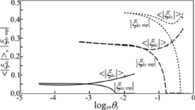
Fig. 25 demonstrates the steady-state probability density (28) for the values of the critical mode amplitude of system (23) in the supercritical region for different values of noise intensity. It can be seen from Fig. 25 that two maxima merge into one at θ1=θ2=5.5×10³subscript𝜃1subscript𝜃25.5superscript103\theta_{1}=\theta_{2}=5.5\times 10^{-3}(dashed line) and bimodal distribution is replaced by unimodal. The plot wst(ξkc)subscript𝑤𝑠𝑡subscript𝜉𝑘𝑐w_{st}(\xi_{kc}) acquires a flat top (plateau). Herewith the steady-state most probable value of the critical mode amplitude module |ξ𝐤cmp|subscript𝜉𝐤𝑐mp{\left|{\xi_{{\mathbf{k}}c\,{\rm{mp}}}}\right|} becomes zero (see Fig. 26). It also follows from Fig. 26 that as the distance from the bifurcation point increases, i.e. with the increase of the bifurcation parameter B, the noise intensity, at which |ξ𝐤cmp|=0subscript𝜉𝐤𝑐mp0{\left|{\xi_{{\mathbf{k}}c\,{\rm{mp}}}}\right|}=0 , increases. The steady-state mean |ξ𝐤c|delimited-⟨⟩subscript𝜉𝐤𝑐{\left\langle{{\left|{\xi_{{\mathbf{k}}c}}\right|}}\right\rangle} is always other than zero and the difference between |ξ𝐤cmp|subscript𝜉𝐤𝑐mp{\left|{\xi_{{\mathbf{k}}c\,{\rm{mp}}}}\right|} and |ξ𝐤c|delimited-⟨⟩subscript𝜉𝐤𝑐{\left\langle{{\left|{\xi_{{\mathbf{k}}c}}\right|}}\right\rangle} increases both with the increase of the noise intensity and that of the parameter B. The latter corresponds to the conclusions from the plots presented in Figs. 16, 20.

Figure 27 illustrates the behavior of the steady-state second order cumulant κ2=ξ𝐤c2/|ξ𝐤c|2subscript𝜅2delimited-⟨⟩superscriptsubscript𝜉𝐤𝑐2superscriptdelimited-⟨⟩subscript𝜉𝐤𝑐2\kappa_{2}={\left\langle{\xi_{\mathbf{k}c}^{2}}\right\rangle}/{{\left\langle|{\xi_{\mathbf{k}c}}|\right\rangle}^{2}} and the susceptibility [ξ𝐤c2|ξ𝐤c|2]/θdelimited-[]delimited-⟨⟩superscriptsubscript𝜉𝐤𝑐2superscriptdelimited-⟨⟩subscript𝜉𝐤𝑐2𝜃[{\left\langle{\xi_{\mathbf{k}c}^{2}}\right\rangle}-{{\left\langle|{\xi_{\mathbf{k}c}}|\right\rangle}^{2}}]/{\theta} of the order parameter as the noise intensity increases at different values of the bifurcation parameter. The second order cumulant is a monotone increasing function at low noise whereas the susceptibility has a marked maximum. This maximum is observed for the values of noise intensity slightly smaller than the values at which |ξ𝐤cmp|=0subscript𝜉𝐤𝑐mp0{\left|{\xi_{{\mathbf{k}}c\,{\rm{mp}}}}\right|}=0 . This maximum can be called a ”forerunner” of a change in the system state.
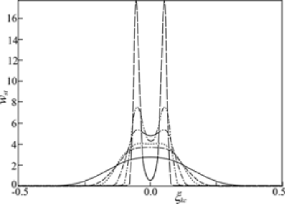
Refer to caption
Figure 25: Steady-state probability density, Eq. (28), for the values of the critical mode amplitude of system (23) in the supercritical region for six values of noise intensity. B𝐵B=5.5. The line with a long dash θ1=θ2=θ=3.5×10⁵subscript𝜃1subscript𝜃2𝜃3.5superscript105\theta_{1}=\theta_{2}=\theta=3.5\times 10^{-5}, the dash-dot-dot line θ=2.0×10⁴𝜃2.0superscript104\theta=2.0\times 10^{-4}, the dash-dot line θ=8.0×10⁴𝜃8.0superscript104\theta=8.0\times 10^{-4}, the dotted line θ=3.0×10³𝜃3.0superscript103\theta=3.0\times 10^{-3}, the dashed line θ=5.5×10³𝜃5.5superscript103\theta=5.5\times 10^{-3}, the solid line θ=2.0×10²𝜃2.0superscript102\theta=2.0\times 10^{-2}.
Refer to caption
Figure 26: Steady-state mean |ξ𝐤c|delimited-⟨⟩subscript𝜉𝐤𝑐{\left\langle{{\left|{\xi_{{\mathbf{k}}c}}\right|}}\right\rangle} and most probable |ξ𝐤cmp|subscript𝜉𝐤𝑐mp{\left|{\xi_{{\mathbf{k}}c\,\rm{mp}}}\right|} values of the critical mode amplitude module as a function of noise intensity. The solid line B𝐵B=5.5, the dashed line B𝐵B=6.0, the dotted line B𝐵B=7.
Refer to caption

a)
Refer to caption
b)

Figure 27: Steady-state second-order cumulant κ2subscript𝜅2\kappa_{2} (a) and susceptibility χ𝜒\chi (b) as functions of noise intensity . θ2=θ1=θsubscript𝜃2subscript𝜃1𝜃\theta_{2}=\theta_{1}=\theta. The solid line B=5.5𝐵5.5B=5.5, the dashed line B=6.0𝐵6.0B=6.0, the dotted line B=7𝐵7B=7.

The analysis of the plots presented in Figs. 14, 18 shows that the steady-state variance of system (23) increases in the region of low noise. This qualitatively corresponds to the areas where the susceptibility of the order parameter in Fig. 27 (b) increases.

One can observe an interesting correspondence between the values of noise intensity at which steady-state bimodal distribution disappears for the critical mode amplitude of system (23) and transient bimodality arises in the ordered phase. We turn to figures 19 and 26. At B𝐵B = 6 these values are 0.16absent0.16\approx 0.16 and 0.090.12absent0.090.12\approx 0.09-0.12 respectively.

V CONCLUSION

Mean field approximation was developed for studying the state of multicomponent stochastic spatially extended systems. We assume that in this case equality (10) is true. Herewith the non-trivial spatial structure, spatial homogeneity, and isotropy of multiplicative noise are taken into account. In this approximation a multivariate single-site nonlinear self-consistent Fokker-Planck equation was derived for probability density of the state of the system under consideration.

The finite-difference method is proposed for the numerical solution of the general class of multivariate nonlinear self-consistent time-dependent Fokker-Planck equations. The accuracy and reliability of the method was illustrated on known one-dimensional problems. It was shown that the method proposed conserves the positive definiteness of solutions and the normalization condition of the probability density unlike the Hermite DAF-based method. In the first order of approximation over time the method proposed makes it possible to obtain solutions with higher accuracy, especially in a steady state and in the region where the solution is close to discontinuity. The necessity of choosing a sufficiently dense uniform grid can be classified as a limitation of the proposed method. However, this can be avoided if the proposed scheme is transferred onto a non-uniform grid.

Mean field approximation was applied to the study of the evolution of the system describing the well-known model of autocatalytic chemical reaction with spatially correlated multiplicative noise. In this paper the region of parameters, in which the Turing bifurcation arises in the deterministic system, was considered. As a result of the numerical study of NSCFPE solutions for a stochastic spatially extended brusselator we found that only unimodal probability distribution (ordered phase) can be observed at low noise intensity. The increase of noise intensity leads to the occurrence of transient bimodality (disordered phase) in the ordered phase. Further growth of noise intensity disrupts the ordering to an even greater extent: ”intermittency” of unimodal and bimodal distribution, that is ”phase intermittency” is observed which ”swings” the ordered state. The behavior of variance over time, the most probable and mean of the function defining the system state in case of increasing the external noise intensity and the bifurcation parameter has been studied. It was shown that the most probable has the discontinuity of the first kind when transient bimodality disappears.

The behavior of the order parameter of the system under consideration was studied. It was shown that some statistical characteristics of the order parameter and the functions defining the system state behave in a similar way in the steady state. Thus, in the vicinity of the bifurcation point the greater the external noise intensity, the greater the variance in the steady state. Simultaneously the increase of noise intensity leads to the increase of difference between the mean and the appropriate most probable in the steady state. It was shown that transient bimodality occurs in the ordered phase when noise intensity values are close to the values corresponding to the transition from bimodal density of steady-state order parameter probability distribution to unimodal one.

ACKNOWLEDGMENTS

The study has been supported by the Ministry of Education and Science of the Russian Federation, state work specification for the years 2014-2016, project No.608, grants of the Russian Foundation for Basic Research 13-01-970050 r_povolzhie_a, 13-01-97001 r_povolzhie_a, 14-02-97030 r_povolzhie_a, and grants of Russian Science Foundation 14-11-00290, 14-12-00472, 14-22-00111.

APPENDIX A


A rectangular spatial mesh ωh=({ih1,jh2})subscript𝜔𝑖subscript1𝑗subscript2\omega_{h}=(\{ih_{1},jh_{2}\}) was chosen for problem (24). Here i,j(i=0,1,,I;j=0,1,,J)𝑖𝑗formulae-sequence𝑖01𝐼𝑗01𝐽i,j\,\,\,(i=0,1,...,I;j=0,1,...,J) and h1,h2subscript1subscript2h_{1},h_{2} are indexes of mesh nodes and steps respectively, and ωτsubscript𝜔𝜏\omega_{\tau} is a temporal mesh with a step τ𝜏\tau on the interval 0tT.0𝑡𝑇0\leq t\leq T. We associate the discrete function wijksuperscriptsubscript𝑤𝑖𝑗𝑘w_{ij}^{k} defined on the mash ωh×ωτsubscript𝜔subscript𝜔𝜏\omega_{h}\times\omega_{\tau} with the continuous function w(x1,x2,t)𝑤subscript𝑥1subscript𝑥2𝑡w(x_{1},x_{2},t).

We choose the initial conditions

w0=w(x1,x2,0)=12πθ1θ2exp{(x1x10)22θ1(x2x20)22θ2},x10=A,x20=B/Aformulae-sequencesubscript𝑤0𝑤subscript𝑥1subscript𝑥2012𝜋subscript𝜃1subscript𝜃2superscriptsubscript𝑥1subscript𝑥1022subscript𝜃1superscriptsubscript𝑥2subscript𝑥2022subscript𝜃2formulae-sequencesubscript𝑥10𝐴subscript𝑥20𝐵𝐴w_{0}=w(x_{1},x_{2},0)={\frac{{1}}{{2\pi\sqrt{\theta_{1}\theta_{2}}}}}\exp{\left\{{-{\frac{{\left({x_{1}-x_{10}}\right)^{2}}}{{2\theta_{1}}}}-{\frac{{\left({x_{2}-x_{20}}\right)^{2}}}{{2\theta_{2}}}}}\right\}},\quad x_{10}=A,\,\,x_{20}=B/A

and boundary conditions w(x1,x2,t)0𝑤subscript𝑥1subscript𝑥2𝑡0w(x_{1},x_{2},t)\to 0 if x1,x2formulae-sequencesubscript𝑥1subscript𝑥2x_{1}\to\infty,x_{2}\to\infty.

A locally one-dimensional scheme (13)-(15) for problem (24) has the form:

wk+α/nwk+(α1)/nτΛαw=0,w0=w0,α=1,2;n=2.formulae-sequencesuperscript𝑤𝑘𝛼𝑛superscript𝑤𝑘𝛼1𝑛𝜏subscriptΛ𝛼𝑤0formulae-sequencesuperscript𝑤0subscript𝑤0formulae-sequence𝛼12𝑛2{\frac{{w^{k+\alpha/n}-w^{k+(\alpha-1)/n}}}{{\tau}}}-\Lambda_{\alpha}w=0,\,\,\,w^{0}=w_{0},\,\,\,\alpha=1,2;\,\,n=2.
Λαw=(aα(qαw)x¯α)xα,subscriptΛ𝛼𝑤subscriptsubscript𝑎𝛼subscriptsubscript𝑞𝛼𝑤subscript¯𝑥𝛼subscript𝑥𝛼\Lambda_{\alpha}w=(a_{\alpha}(q_{\alpha}w)_{\bar{x}_{\alpha}})_{x_{\alpha}},\,\,
q1=exp(a0x1+a1ln|x1|x1x2θ1),q2=exp(b1(x1)x2+b2(x1)x22),formulae-sequencesubscript𝑞1subscript𝑎0subscript𝑥1subscript𝑎1subscript𝑥1subscript𝑥1subscript𝑥2subscript𝜃1subscript𝑞2subscript𝑏1subscript𝑥1subscript𝑥2subscript𝑏2subscript𝑥1superscriptsubscript𝑥22q_{1}=\exp\left({{\frac{{a_{0}}}{{x_{1}}}}+a_{1}\ln{\left|{x_{1}}\right|}\,\,-{\frac{{x_{1}x_{2}}}{{\theta_{1}}}}}\right),q_{2}=\exp\left({-b_{1}(x_{1})x_{2}+b_{2}(x_{1})x_{2}^{2}}\right),
a1,i={12θ1[exp(a0x1,ix1,ix2θ1)x1,ia12+exp(a0x1,i1x1,i1x2θ1)x1,i1a12]}1,x1,i=ih1,formulae-sequencesubscript𝑎1𝑖superscript12subscript𝜃1delimited-[]subscript𝑎0subscript𝑥1𝑖subscript𝑥1𝑖subscript𝑥2subscript𝜃1superscriptsubscript𝑥1𝑖subscript𝑎12subscript𝑎0subscript𝑥1𝑖1subscript𝑥1𝑖1subscript𝑥2subscript𝜃1superscriptsubscript𝑥1𝑖1subscript𝑎121subscript𝑥1𝑖𝑖subscript1a_{1,i}={\left\{{{\frac{{1}}{{2\theta_{1}}}}{\left[{\exp\left({{\frac{{a_{0}}}{{x_{1,i}}}}-{\frac{{x_{1,i}x_{2}}}{{\theta_{1}}}}}\right)x_{1,i}^{a_{1}-2}+\exp\left({{\frac{{a_{0}}}{{x_{1,i-1}}}}-{\frac{{x_{1,i-1}x_{2}}}{{\theta_{1}}}}}\right)x_{1,i-1}^{a_{1}-2}}\right]}}\right\}}^{-1},x_{1,i}=ih_{1},
a2,j={12θ2x12[exp(b1(x1)x2,j+b2(x1)x2,j2)+exp(b1(x1)x2,j1+b2(x1)x2,j12)]}1,x2,j=jh2.formulae-sequencesubscript𝑎2𝑗superscript12subscript𝜃2superscriptsubscript𝑥12delimited-[]subscript𝑏1subscript𝑥1subscript𝑥2𝑗subscript𝑏2subscript𝑥1superscriptsubscript𝑥2𝑗2subscript𝑏1subscript𝑥1subscript𝑥2𝑗1subscript𝑏2subscript𝑥1superscriptsubscript𝑥2𝑗121subscript𝑥2𝑗𝑗subscript2a_{2,j}={\left\{{{\frac{{1}}{{2\theta_{2}x_{1}^{2}}}}{\left[{\exp\left({-b_{1}(x_{1})x_{2,j}+b_{2}(x_{1})x_{2,j}^{2}}\right)+\exp\left({-b_{1}(x_{1})x_{2,j-1}+b_{2}(x_{1})x_{2,j-1}^{2}}\right)}\right]}}\right\}}^{-1},x_{2,j}=jh_{2}.

Here the notations are introduced:

a0=A+D1E(x1|x2,t)θ1,a1=B+1+θ1+D1θ1,b1(x1)=Bθ2x1+D2E(x2|x1,t)θ2x12,b2(x1)=x12+D22θ2x12.formulae-sequencesubscript𝑎0𝐴subscript𝐷1𝐸conditionalsubscript𝑥1subscript𝑥2𝑡subscript𝜃1subscript𝑎1𝐵1subscript𝜃1subscript𝐷1subscript𝜃1formulae-sequencesubscript𝑏1subscript𝑥1𝐵subscript𝜃2subscript𝑥1subscript𝐷2𝐸conditionalsubscript𝑥2subscript𝑥1𝑡subscript𝜃2superscriptsubscript𝑥12subscript𝑏2subscript𝑥1superscriptsubscript𝑥12subscript𝐷22subscript𝜃2superscriptsubscript𝑥12\begin{array}[]{l}a_{0}={\frac{{A+D_{1}E(x_{1}|x_{2},t)}}{{\theta_{1}}}},\,\,\,\,\,\,\,\,\,\,\,\,\,\,\,\,\,\,\,\,\,\,\,\,\,\,\,\,\,a_{1}={\frac{{B+1+\theta_{1}+D_{1}}}{{\theta_{1}}}},\\ b_{1}(x_{1})={\frac{{B}}{{\theta_{2}x_{1}}}}+{\frac{{D_{2}E(x_{2}|x_{1},t)}}{{\theta_{2}x_{1}^{2}}}},\,\,\,\,\,\,\,\,\,\,\,\,\,\,\,b_{2}(x_{1})={\frac{{x_{1}^{2}+D_{2}}}{{2\theta_{2}x_{1}^{2}}}}.\\ \end{array}

On the boundary:

w1jk=w0jk0,wi 1k=wi 0k0,wIjk=wI1jk0,wiJk=wiJ1k0.formulae-sequencesuperscriptsubscript𝑤1𝑗𝑘superscriptsubscript𝑤0𝑗𝑘similar-to0superscriptsubscript𝑤𝑖1𝑘superscriptsubscript𝑤𝑖 0𝑘similar-to0superscriptsubscript𝑤𝐼𝑗𝑘superscriptsubscript𝑤𝐼1𝑗𝑘similar-to0superscriptsubscript𝑤𝑖𝐽𝑘superscriptsubscript𝑤𝑖𝐽1𝑘similar-to0w_{1j}^{k}=w_{0j}^{k}\sim 0,\,\,w_{i\,1}^{k}=w_{i\,0}^{k}\sim 0,w_{Ij}^{k}=w_{I-1j}^{k}\sim 0,\,\,w_{i\,J}^{k}=w_{i\,J-1}^{k}\sim 0.

At the transition to a semilayer:

Biwi+1jk+1/2+Ciwijk+1/2Aiwi1jk+1/2=wijk.subscript𝐵𝑖superscriptsubscript𝑤𝑖1𝑗𝑘12subscript𝐶𝑖superscriptsubscript𝑤𝑖𝑗𝑘12subscript𝐴𝑖superscriptsubscript𝑤𝑖1𝑗𝑘12superscriptsubscript𝑤𝑖𝑗𝑘-B_{i}w_{i+1j}^{k+1/2}+C_{i}w_{i\,j}^{k+1/2}-A_{i}w_{i-1\,j}^{k+1/2}=w_{i\,j}^{k}.
A0=0;B0=1;C0=1;F0=0.AI=1;BI=0;CI=1;FI=0.A_{0}=0;\,B_{0}=1;\,C_{0}=1;F_{0}=0.\quad A_{I}=1;\,B_{I}=0;\,C_{I}=1;F_{I}=0.
Ai=τθ1h12|x1h1|21+exp{a0h1x1(x1h1)x2h1θ1+(a12)ln|x1x1h1|},Bi=τθ1h12|x1+h1|21+exp{a0h1x1(x1+h1)+x2h1θ1+(a12)ln|x1x1+h1|},Ci=1++τθ1x12h1211+exp{a0h1x1(x1+h1)x2h1θ1+(a12)ln|x1+h1x1|}+τθ1x12h1211+exp{a0h1x1(x1h1)+x2h1θ1+(a12)ln|x1h1x1|}subscript𝐴𝑖𝜏subscript𝜃1superscriptsubscript12superscriptsubscript𝑥1subscript121subscript𝑎0subscript1subscript𝑥1subscript𝑥1subscript1subscript𝑥2subscript1subscript𝜃1subscript𝑎12subscript𝑥1subscript𝑥1subscript1subscript𝐵𝑖𝜏subscript𝜃1superscriptsubscript12superscriptsubscript𝑥1subscript121subscript𝑎0subscript1subscript𝑥1subscript𝑥1subscript1subscript𝑥2subscript1subscript𝜃1subscript𝑎12subscript𝑥1subscript𝑥1subscript1subscript𝐶𝑖limit-from1limit-from𝜏subscript𝜃1superscriptsubscript𝑥12superscriptsubscript1211subscript𝑎0subscript1subscript𝑥1subscript𝑥1subscript1subscript𝑥2subscript1subscript𝜃1subscript𝑎12subscript𝑥1subscript1subscript𝑥1𝜏subscript𝜃1superscriptsubscript𝑥12superscriptsubscript1211subscript𝑎0subscript1subscript𝑥1subscript𝑥1subscript1subscript𝑥2subscript1subscript𝜃1subscript𝑎12subscript𝑥1subscript1subscript𝑥1\begin{array}[]{l}A_{i}={\frac{{\tau\theta_{1}}}{{h_{1}^{2}}}}{\frac{{{\left|{x_{1}-h_{1}}\right|}^{2}}}{{1+\exp{\left\{{-{\frac{{a_{0}h_{1}}}{{x_{1}(x_{1}-h_{1})}}}-{\frac{{x_{2}h_{1}}}{{\theta_{1}}}}+(a_{1}-2)\ln{\left|{{\frac{{x_{1}}}{{x_{1}-h_{1}}}}}\right|}}\right\}}}}},\\ B_{i}={\frac{{\tau\theta_{1}}}{{h_{1}^{2}}}}{\frac{{{\left|{x_{1}+h_{1}}\right|}^{2}}}{{1+\exp{\left\{{{\frac{{a_{0}h_{1}}}{{x_{1}(x_{1}+h_{1})}}}+{\frac{{x_{2}h_{1}}}{{\theta_{1}}}}+(a_{1}-2)\ln{\left|{{\frac{{x_{1}}}{{x_{1}+h_{1}}}}}\right|}}\right\}}}}},\\ C_{i}=1+\\ +{\frac{{\tau\theta_{1}x_{1}^{2}}}{{h_{1}^{2}}}}{\frac{{1}}{{1+\exp{\left\{{-{\frac{{a_{0}h_{1}}}{{x_{1}(x_{1}+h_{1})}}}-{\frac{{x_{2}h_{1}}}{{\theta_{1}}}}+(a_{1}-2)\ln{\left|{{\frac{{x_{1}+h_{1}}}{{x_{1}}}}}\right|}}\right\}}}}}+\\ {\frac{{\tau\theta_{1}x_{1}^{2}}}{{h_{1}^{2}}}}{\frac{{1}}{{1+\exp{\left\{{{\frac{{a_{0}h_{1}}}{{x_{1}(x_{1}-h_{1})}}}+{\frac{{x_{2}h_{1}}}{{\theta_{1}}}}+(a_{1}-2)\ln{\left|{{\frac{{x_{1}-h_{1}}}{{x_{1}}}}}\right|}}\right\}}}}}\\ \end{array}

At the transition to a whole layer:

Bjwij+1k+1+Cjwijk+1Ajwij1k+1=wijk+1/2.subscript𝐵𝑗superscriptsubscript𝑤𝑖𝑗1𝑘1subscript𝐶𝑗superscriptsubscript𝑤𝑖𝑗𝑘1subscript𝐴𝑗superscriptsubscript𝑤𝑖𝑗1𝑘1superscriptsubscript𝑤𝑖𝑗𝑘12-B_{j}w_{i\,j+1}^{k+1}+C_{j}w_{i\,j}^{k+1}-A_{j}w_{i\,j-1}^{k+1}=w_{i\,j}^{k+1/2}.
A0=0;B0=1;C0=1;F0=0.AJ=1;BJ=0;CJ=1;FJ=0.A_{0}=0;\,B_{0}=1;\,C_{0}=1;F_{0}=0.\quad A_{J}=1;\,B_{J}=0;\,C_{J}=1;F_{J}=0.
Aj=τθ2x12h2211+exp{b1h2+2b2h2(x20.5h2)},Bj=τθ2x12h2211+exp{b1h22b2h2(x2+0.5h2)},Cj=1+τθ2x12h12[11+exp{b1h2+2b2h2(x2+0.5h2)}+11+exp{b1h22b2h2(x20.5h2)}].subscript𝐴𝑗𝜏subscript𝜃2superscriptsubscript𝑥12superscriptsubscript2211subscript𝑏1subscript22subscript𝑏2subscript2subscript𝑥20.5subscript2subscript𝐵𝑗𝜏subscript𝜃2superscriptsubscript𝑥12superscriptsubscript2211subscript𝑏1subscript22subscript𝑏2subscript2subscript𝑥20.5subscript2subscript𝐶𝑗1𝜏subscript𝜃2superscriptsubscript𝑥12superscriptsubscript12delimited-[]11subscript𝑏1subscript22subscript𝑏2subscript2subscript𝑥20.5subscript211subscript𝑏1subscript22subscript𝑏2subscript2subscript𝑥20.5subscript2\begin{array}[]{l}A_{j}={\frac{{\tau\theta_{2}x_{1}^{2}}}{{h_{2}^{2}}}}{\frac{{1}}{{1+\exp{\left\{{-b_{1}h_{2}+2b_{2}h_{2}(x_{2}-0.5h_{2})}\right\}}}}},\\ B_{j}={\frac{{\tau\theta_{2}x_{1}^{2}}}{{h_{2}^{2}}}}{\frac{{1}}{{1+\exp{\left\{{b_{1}h_{2}-2b_{2}h_{2}(x_{2}+0.5h_{2})}\right\}}}}},\\ C_{j}=1+{\frac{{\tau\theta_{2}x_{1}^{2}}}{{h_{1}^{2}}}}{\left[{{\frac{{1}}{{1+\exp{\left\{{-b_{1}h_{2}+2b_{2}h_{2}(x_{2}+0.5h_{2})}\right\}}}}}+{\frac{{1}}{{1+\exp{\left\{{b_{1}h_{2}-2b_{2}h_{2}(x_{2}-0.5h_{2})}\right\}}}}}}\right]}.\\ \end{array}

APPENDIX B


The functions introduced in Eq.(25):

λμ(𝐤)=α(𝐤)2±α2(𝐤)4β(𝐤),subscript𝜆𝜇𝐤plus-or-minus𝛼𝐤2superscript𝛼2𝐤4𝛽𝐤\lambda_{\mu}({\mathbf{k}})={\frac{{\alpha({\mathbf{k}})}}{{2}}}\pm\sqrt{{\frac{{\alpha^{2}({\mathbf{k}})}}{{4}}}-\beta({\mathbf{k}})},
α(𝐤)=B1A2(D1+D2)k2,β(𝐤)=[A2D1(B1)D2]k2+D1D2k4+A2,formulae-sequence𝛼𝐤𝐵1superscript𝐴2subscript𝐷1subscript𝐷2superscript𝑘2𝛽𝐤delimited-[]superscript𝐴2subscript𝐷1𝐵1subscript𝐷2superscript𝑘2subscript𝐷1subscript𝐷2superscript𝑘4superscript𝐴2\alpha({\mathbf{k}})=B-1-A^{2}-(D_{1}+D_{2})k^{2},\\ \beta({\mathbf{k}})=[A^{2}D_{1}-(B-1)D_{2}]k^{2}+D_{1}D_{2}k^{4}+A^{2},\\
Ω1(𝐤u,𝐤u,𝐤s,𝐳(τ))=μ,φηφ(μ)(𝐤u,𝐤u)zφ,𝐤u𝐤u𝐤sμ,φ,φAφφ(μ)(𝐤u,𝐤s,𝐤u)zφ,𝐤u𝐤szφ,𝐤s𝐤u,subscriptΩ1subscript𝐤𝑢subscriptsuperscript𝐤𝑢subscript𝐤𝑠𝐳𝜏subscript𝜇𝜑superscriptsubscript𝜂𝜑𝜇subscript𝐤𝑢subscriptsuperscript𝐤𝑢subscript𝑧𝜑𝐤𝑢superscript𝐤𝑢subscriptsuperscript𝐤𝑠subscript𝜇𝜑superscript𝜑superscriptsubscript𝐴𝜑superscript𝜑𝜇subscriptsuperscript𝐤𝑢subscript𝐤𝑠subscript𝐤𝑢subscript𝑧𝜑𝐤𝑢𝐤𝑠subscript𝑧superscript𝜑𝐤𝑠superscript𝐤𝑢\Omega_{1}({\mathbf{k}}_{u},{\mathbf{k}^{\prime}}_{u},{\mathbf{k}}_{s},{\mathbf{z}}(\tau))={\sum\limits_{\mu,\varphi}{\eta_{\varphi}^{(\mu)}({\mathbf{k}}_{u},{\mathbf{k}^{\prime}}_{u})z_{\varphi,{\mathbf{k}}u-{\mathbf{k}^{\prime}}u}}}-{\sum\limits_{{\mathbf{k}^{\prime}}s}{{\sum\limits_{\mu,\varphi,{\varphi}^{\prime}}{A_{\varphi{\varphi}^{\prime}}^{(\mu)}({\mathbf{k}^{\prime}}_{u},{\mathbf{k}}_{s},{\mathbf{k}}_{u})z_{\varphi,{\mathbf{k}}u-{\mathbf{k}}s}z_{{\varphi}^{\prime},{\mathbf{k}}s-{\mathbf{k}^{\prime}}u}}}}},
Ω11(𝐤u,𝐤u,𝐤′′u,𝐤s,𝐳(τ))=δ(𝐤u,𝐤u,𝐤′′u)μ,φ(1)φνφ(μ)(𝐤u,𝐤u,𝐤′′u)zφ,𝐤u𝐤u𝐤′′u,subscriptΩ11subscript𝐤𝑢subscriptsuperscript𝐤𝑢subscriptsuperscript𝐤′′𝑢subscript𝐤𝑠𝐳𝜏𝛿subscript𝐤𝑢subscriptsuperscript𝐤𝑢subscriptsuperscript𝐤′′𝑢subscript𝜇𝜑superscript1𝜑superscriptsubscript𝜈𝜑𝜇subscript𝐤𝑢subscriptsuperscript𝐤𝑢subscriptsuperscript𝐤′′𝑢subscript𝑧𝜑𝐤𝑢superscript𝐤𝑢superscript𝐤′′𝑢\Omega_{11}({\mathbf{k}}_{u},{\mathbf{k}^{\prime}}_{u},{\mathbf{k}^{\prime\prime}}_{u},{\mathbf{k}}_{s},{\mathbf{z}}(\tau))=\delta({\mathbf{k}}_{u},{\mathbf{k}^{\prime}}_{u},{\mathbf{k}^{\prime\prime}}_{u})-{\sum\limits_{\mu,\varphi}{(-1)^{\varphi}\nu_{\varphi}^{(\mu)}({\mathbf{k}}_{u},{\mathbf{k}^{\prime}}_{u},{\mathbf{k}^{\prime\prime}}_{u})z_{\varphi,{\mathbf{k}}u-{\mathbf{k}^{\prime}}u-{\mathbf{k}^{\prime\prime}}u}}},
ηφ(μ)(𝐤u,𝐤u)=(1)φ[O1(1)(𝐤u)Oφ(1)(𝐤u)βφ(μ)(𝐤u,𝐤u)],superscriptsubscript𝜂𝜑𝜇subscript𝐤𝑢subscriptsuperscript𝐤𝑢superscript1𝜑delimited-[]superscriptsubscript𝑂11subscriptsuperscript𝐤𝑢superscriptsubscript𝑂𝜑absent1subscript𝐤𝑢superscriptsubscript𝛽𝜑𝜇subscript𝐤𝑢subscriptsuperscript𝐤𝑢\eta_{\varphi}^{(\mu)}({\mathbf{k}}_{u},{\mathbf{k}^{\prime}}_{u})=(-1)^{\varphi}[O_{1}^{(1)}({\mathbf{k}^{\prime}}_{u})O_{\varphi}^{*(1)}({\mathbf{k}}_{u})-\beta_{\varphi}^{(\mu)}({\mathbf{k}}_{u},{\mathbf{k}^{\prime}}_{u})],
Aφφ(μ)(𝐤u,𝐤s,𝐤u)=(1)φ+φO1(1)(𝐤u)εφφ(μ)(𝐤s,𝐤u),superscriptsubscript𝐴𝜑superscript𝜑𝜇subscriptsuperscript𝐤𝑢subscript𝐤𝑠subscript𝐤𝑢superscript1𝜑superscript𝜑superscriptsubscript𝑂11subscriptsuperscript𝐤𝑢superscriptsubscript𝜀𝜑superscript𝜑𝜇subscript𝐤𝑠subscriptsuperscript𝐤𝑢A_{\varphi{\varphi}^{\prime}}^{(\mu)}({\mathbf{k}^{\prime}}_{u},{\mathbf{k}}_{s},{\mathbf{k}}_{u})=(-1)^{\varphi+{\varphi}^{\prime}}O_{1}^{(1)}({\mathbf{k}^{\prime}}_{u})\varepsilon_{\varphi{\varphi}^{\prime}}^{(\mu)}({\mathbf{k}}_{s},{\mathbf{k}^{\prime}}_{u}),
ζφφ(μ)(𝐤s,𝐤u)=(1)φ+φAεφφ(μ)(𝐤s,𝐤u),superscriptsubscript𝜁𝜑superscript𝜑𝜇subscript𝐤𝑠subscript𝐤𝑢superscript1𝜑superscript𝜑𝐴superscriptsubscript𝜀𝜑superscript𝜑𝜇subscript𝐤𝑠subscriptsuperscript𝐤𝑢\zeta_{\varphi{\varphi}^{\prime}}^{(\mu)}({\mathbf{k}}_{s},{\mathbf{k}}_{u})=(-1)^{\varphi+{\varphi}^{\prime}}A\varepsilon_{\varphi{\varphi}^{\prime}}^{(\mu)}({\mathbf{k}}_{s},{\mathbf{k}^{\prime}}_{u}),
εφφ(μ)(𝐤s,𝐤u)=O1(μ)(𝐤s)λμ(𝐤s)Oφ(μ)(𝐤s)Oφ(1)(𝐤u),superscriptsubscript𝜀𝜑superscript𝜑𝜇subscript𝐤𝑠subscriptsuperscript𝐤𝑢superscriptsubscript𝑂1𝜇subscript𝐤𝑠subscript𝜆𝜇subscript𝐤𝑠superscriptsubscript𝑂𝜑absent𝜇subscript𝐤𝑠superscriptsubscript𝑂superscript𝜑absent1subscript𝐤𝑢\varepsilon_{\varphi{\varphi}^{\prime}}^{(\mu)}({\mathbf{k}}_{s},{\mathbf{k}^{\prime}}_{u})={\frac{{O_{1}^{(\mu)}({\mathbf{k}}_{s})}}{{\lambda_{\mu}({\mathbf{k}}_{s})}}}O_{\varphi}^{*(\mu)}({\mathbf{k}}_{s})O_{{\varphi}^{\prime}}^{*(1)}({\mathbf{k}}_{u}),
βφ(μ)(𝐤u,𝐤u)=O1(1)(𝐤u)O2(1)(𝐤u)λμ(|𝐤u𝐤u|)Oφ(μ)(|𝐤u𝐤u|)σ1μ(𝐤u,|𝐤u𝐤u|),superscriptsubscript𝛽𝜑𝜇subscript𝐤𝑢subscriptsuperscript𝐤𝑢superscriptsubscript𝑂1absent1subscript𝐤𝑢superscriptsubscript𝑂2absent1subscript𝐤𝑢subscript𝜆𝜇subscript𝐤𝑢subscriptsuperscript𝐤𝑢superscriptsubscript𝑂𝜑absent𝜇subscript𝐤𝑢subscriptsuperscript𝐤𝑢superscript𝜎1𝜇subscript𝐤𝑢subscript𝐤𝑢subscriptsuperscript𝐤𝑢\beta_{\varphi}^{(\mu)}({\mathbf{k}}_{u},{\mathbf{k}^{\prime}}_{u})={\frac{{O_{1}^{*(1)}({\mathbf{k}}_{u})-O_{2}^{*(1)}({\mathbf{k}}_{u})}}{{\lambda_{\mu}({\left|{{\mathbf{k}}_{u}-{\mathbf{k}^{\prime}}_{u}}\right|})}}}O_{\varphi}^{*(\mu)}({\left|{{\mathbf{k}}_{u}-{\mathbf{k}^{\prime}}_{u}}\right|})\sigma^{1\mu}({\mathbf{k}}_{u},{\left|{{\mathbf{k}}_{u}-{\mathbf{k}^{\prime}}_{u}}\right|}),
νφ(μ)(𝐤u,𝐤u,𝐤′′u)=βφ(μ)(𝐤u,𝐤u)O1(1)(𝐤′′u)+superscriptsubscript𝜈𝜑𝜇subscript𝐤𝑢subscriptsuperscript𝐤𝑢subscriptsuperscript𝐤′′𝑢limit-fromsuperscriptsubscript𝛽𝜑𝜇subscript𝐤𝑢subscriptsuperscript𝐤𝑢superscriptsubscript𝑂11subscriptsuperscript𝐤′′𝑢\nu_{\varphi}^{(\mu)}({\mathbf{k}}_{u},{\mathbf{k}^{\prime}}_{u},{\mathbf{k}^{\prime\prime}}_{u})=\beta_{\varphi}^{(\mu)}({\mathbf{k}}_{u},{\mathbf{k}^{\prime}}_{u})O_{1}^{(1)}({\mathbf{k}^{\prime\prime}}_{u})+
Oφ(1)(𝐤u)O1(μ)(|𝐤u+𝐤′′|u)λμ(|𝐤u+𝐤′′u|)[O1(μ)(|𝐤u+𝐤′′u|)O_{\varphi}^{*(1)}({\mathbf{k}}_{u}){\frac{{O_{1}^{(\mu)}({\left|{{\mathbf{k}^{\prime}}_{u}+{\mathbf{k}^{\prime\prime}}}\right|}_{u})}}{{\lambda_{\mu}({\left|{{\mathbf{k}^{\prime}}_{u}+{\mathbf{k}^{\prime\prime}}_{u}}\right|})}}}[O_{1}^{*(\mu)}({\left|{{\mathbf{k}^{\prime}}_{u}+{\mathbf{k}^{\prime\prime}}_{u}}\right|})-
O2(μ)(|𝐤u+𝐤′′u|)][2AO1(1)(𝐤u)O2(1)(𝐤′′u)+BAO1(1)(𝐤u)O1(1)(𝐤′′u)],O_{2}^{*(\mu)}({\left|{{\mathbf{k}^{\prime}}_{u}+{\mathbf{k}^{\prime\prime}}_{u}}\right|})][2AO_{1}^{(1)}({\mathbf{k}^{\prime}}_{u})O_{2}^{(1)}({\mathbf{k}^{\prime\prime}}_{u})+{\frac{{B}}{{A}}}O_{1}^{(1)}({\mathbf{k}^{\prime}}_{u})O_{1}^{(1)}({\mathbf{k}^{\prime\prime}}_{u})],\\
δ(𝐤u,𝐤u,𝐤′′u)=[O1(1)(𝐤u)O2(1)(𝐤u)][2AO1(1)(𝐤u)O2(1)(𝐤′′u)+BAO1(1)(𝐤u)O1(1)(𝐤′′u)]δ(𝐤u𝐤u𝐤′′u),𝛿subscript𝐤𝑢subscriptsuperscript𝐤𝑢subscriptsuperscript𝐤′′𝑢delimited-[]superscriptsubscript𝑂1absent1subscript𝐤𝑢superscriptsubscript𝑂2absent1subscript𝐤𝑢delimited-[]2𝐴superscriptsubscript𝑂11subscriptsuperscript𝐤𝑢superscriptsubscript𝑂21subscriptsuperscript𝐤′′𝑢𝐵𝐴superscriptsubscript𝑂11subscriptsuperscript𝐤𝑢superscriptsubscript𝑂11subscriptsuperscript𝐤′′𝑢𝛿subscript𝐤𝑢subscriptsuperscript𝐤𝑢subscriptsuperscript𝐤′′𝑢\delta({\mathbf{k}}_{u},{\mathbf{k}^{\prime}}_{u},{\mathbf{k}^{\prime\prime}}_{u})=[O_{1}^{*(1)}({\mathbf{k}}_{u})-O_{2}^{*(1)}({\mathbf{k}}_{u})][2AO_{1}^{(1)}({\mathbf{k}^{\prime}}_{u})O_{2}^{(1)}({\mathbf{k}^{\prime\prime}}_{u})+{\frac{{B}}{{A}}}O_{1}^{(1)}({\mathbf{k}^{\prime}}_{u})O_{1}^{(1)}({\mathbf{k}^{\prime\prime}}_{u})]\delta({\mathbf{k}}_{u}-{\mathbf{k}^{\prime}}_{u}-{\mathbf{k}^{\prime\prime}}_{u}),
ω(𝐤u,𝐤u,𝐤′′u,𝐤′′′u)=[O1(1)(𝐤u)O2(1)(𝐤u)]O1(1)(𝐤u)O1(1)(𝐤′′u)O2(1)(𝐤′′′u)δ(𝐤u𝐤u𝐤′′u𝐤′′′u)𝜔subscript𝐤𝑢subscriptsuperscript𝐤𝑢subscriptsuperscript𝐤′′𝑢subscriptsuperscript𝐤′′′𝑢limit-fromdelimited-[]superscriptsubscript𝑂1absent1subscript𝐤𝑢superscriptsubscript𝑂2absent1subscript𝐤𝑢superscriptsubscript𝑂11subscriptsuperscript𝐤𝑢superscriptsubscript𝑂11subscriptsuperscript𝐤′′𝑢superscriptsubscript𝑂21subscriptsuperscript𝐤′′′𝑢𝛿subscript𝐤𝑢subscriptsuperscript𝐤𝑢subscriptsuperscript𝐤′′𝑢subscriptsuperscript𝐤′′′𝑢\omega({\mathbf{k}}_{u},{\mathbf{k}^{\prime}}_{u},{\mathbf{k}^{\prime\prime}}_{u},{\mathbf{k}^{\prime\prime\prime}}_{u})=[O_{1}^{*(1)}({\mathbf{k}}_{u})-O_{2}^{*(1)}({\mathbf{k}}_{u})]O_{1}^{(1)}({\mathbf{k}^{\prime}}_{u})O_{1}^{(1)}({\mathbf{k}^{\prime\prime}}_{u})O_{2}^{(1)}({\mathbf{k}^{\prime\prime\prime}}_{u})\delta({\mathbf{k}}_{u}-{\mathbf{k}^{\prime}}_{u}-{\mathbf{k}^{\prime\prime}}_{u}-{\mathbf{k}^{\prime\prime\prime}}_{u})-
𝐤s,μ{[O1(1)(𝐤u)O2(1)(𝐤u)]λμ(𝐤s)σ1μ(𝐤u,𝐤s)[O1(μ)(𝐤s)O2(μ)(𝐤s)]×{\sum\limits_{{\mathbf{k}}s,\mu}{{\left\{{{\frac{{[O_{1}^{*(1)}({\mathbf{k}}_{u})-O_{2}^{*(1)}({\mathbf{k}}_{u})]}}{{\lambda_{\mu}({\mathbf{k}}_{s})}}}\sigma^{1\mu}({\mathbf{k}^{\prime}}_{u},{\mathbf{k}}_{s})[O_{1}^{*(\mu)}({\mathbf{k}}_{s})-O_{2}^{*(\mu)}({\mathbf{k}}_{s})]}\right.}}}\times
[2AO1(1)(𝐤′′′u)O2(1)(𝐤′′u)+BAO1(1)(𝐤′′′u)O1(1)(𝐤′′u)]δ(𝐤u𝐤u𝐤s)δ(𝐤s𝐤′′u𝐤′′′u)},{\left.{[2AO_{1}^{(1)}({\mathbf{k}^{\prime\prime\prime}}_{u})O_{2}^{(1)}({\mathbf{k}^{\prime\prime}}_{u})+{\frac{{B}}{{A}}}O_{1}^{(1)}({\mathbf{k}^{\prime\prime\prime}}_{u})O_{1}^{(1)}({\mathbf{k}^{\prime\prime}}_{u})]\delta({\mathbf{k}}_{u}-{\mathbf{k}^{\prime}}_{u}-{\mathbf{k}}_{s})\delta({\mathbf{k}}_{s}-{\mathbf{k}^{\prime\prime}}_{u}-{\mathbf{k}^{\prime\prime\prime}}_{u})}\right\}},
σ1μ(𝐤u,𝐤s)=2AO1(1)(𝐤u)O2(μ)(𝐤s)+2BAO1(1)(𝐤u)O1(μ)(𝐤s)+2AO1(μ)(𝐤s)O2(1)(𝐤u),superscript𝜎1𝜇subscriptsuperscript𝐤𝑢subscript𝐤𝑠2𝐴superscriptsubscript𝑂11subscriptsuperscript𝐤𝑢superscriptsubscript𝑂2𝜇subscript𝐤𝑠2𝐵𝐴superscriptsubscript𝑂11subscriptsuperscript𝐤𝑢superscriptsubscript𝑂1𝜇subscript𝐤𝑠2𝐴superscriptsubscript𝑂1𝜇subscript𝐤𝑠superscriptsubscript𝑂21subscriptsuperscript𝐤𝑢\sigma^{1\mu}({\mathbf{k}^{\prime}}_{u},{\mathbf{k}}_{s})=2AO_{1}^{(1)}({\mathbf{k}^{\prime}}_{u})O_{2}^{(\mu)}({\mathbf{k}}_{s})+2{\frac{{B}}{{A}}}O_{1}^{(1)}({\mathbf{k}^{\prime}}_{u})O_{1}^{(\mu)}({\mathbf{k}}_{s})+2AO_{1}^{(\mu)}({\mathbf{k}}_{s})O_{2}^{(1)}({\mathbf{k}^{\prime}}_{u}),
𝐎(μ)(𝐤)=((A2D2k2λμ(𝐤))/B1),𝐎(μ)(𝐤)=((1)μO2(μ)(𝐤)/[O2(1)(𝐤)O1(2)(𝐤)O2(2)(𝐤)O1(1)(𝐤)](1)μO1(μ)(𝐤)/[O2(1)(𝐤)O1(2)(𝐤)O2(1)(𝐤)O1(1)(𝐤)]),ifμ=1,μ=2;ifμ=2,μ=1.superscript𝐎𝜇𝐤superscript𝐴2subscript𝐷2superscript𝑘2subscript𝜆𝜇𝐤𝐵missing-subexpressionmissing-subexpressionmissing-subexpressionmissing-subexpressionmissing-subexpressionmissing-subexpressionmissing-subexpressionmissing-subexpressionmissing-subexpressionmissing-subexpressionmissing-subexpressionmissing-subexpressionmissing-subexpressionmissing-subexpressionmissing-subexpressionmissing-subexpressionmissing-subexpressionmissing-subexpressionmissing-subexpression1missing-subexpressionmissing-subexpressionmissing-subexpressionmissing-subexpressionmissing-subexpressionmissing-subexpressionmissing-subexpressionmissing-subexpressionmissing-subexpressionmissing-subexpressionmissing-subexpressionmissing-subexpressionmissing-subexpressionmissing-subexpressionmissing-subexpressionmissing-subexpressionmissing-subexpressionmissing-subexpressionmissing-subexpressionformulae-sequencesuperscript𝐎absent𝜇𝐤superscript1𝜇superscriptsubscript𝑂2superscript𝜇𝐤delimited-[]superscriptsubscript𝑂21𝐤superscriptsubscript𝑂12𝐤superscriptsubscript𝑂22𝐤superscriptsubscript𝑂11𝐤missing-subexpressionmissing-subexpressionmissing-subexpressionmissing-subexpressionmissing-subexpressionmissing-subexpressionmissing-subexpressionmissing-subexpressionmissing-subexpressionmissing-subexpressionmissing-subexpressionmissing-subexpressionmissing-subexpressionmissing-subexpressionmissing-subexpressionmissing-subexpressionmissing-subexpressionmissing-subexpressionmissing-subexpressionsuperscript1superscript𝜇superscriptsubscript𝑂1superscript𝜇𝐤delimited-[]superscriptsubscript𝑂21𝐤superscriptsubscript𝑂12𝐤superscriptsubscript𝑂21𝐤superscriptsubscript𝑂11𝐤missing-subexpressionmissing-subexpressionmissing-subexpressionmissing-subexpressionmissing-subexpressionmissing-subexpressionmissing-subexpressionmissing-subexpressionmissing-subexpressionmissing-subexpressionmissing-subexpressionmissing-subexpressionmissing-subexpressionmissing-subexpressionmissing-subexpressionmissing-subexpressionmissing-subexpressionmissing-subexpressionmissing-subexpressionformulae-sequenceif𝜇1formulae-sequencesuperscript𝜇2formulae-sequenceif𝜇2superscript𝜇1\begin{array}[]{l}{\mathbf{O}}^{(\mu)}({\mathbf{k}})=\left({{\begin{array}[]{*{20}c}{(-A^{2}-D_{2}k^{2}-\lambda_{\mu}({\mathbf{k}}))/B\hfill}\\ {1\hfill}\\ \end{array}}}\right),\\ {\mathbf{O}}^{*(\mu)}({\mathbf{k}})=\left({{\begin{array}[]{*{20}c}{(-1)^{\mu}O_{2}^{({\mu}^{\prime})}({\mathbf{k}})/[O_{2}^{(1)}({\mathbf{k}})O_{1}^{(2)}({\mathbf{k}})-O_{2}^{(2)}({\mathbf{k}})O_{1}^{(1)}({\mathbf{k}})]\hfill}\\ {(-1)^{{\mu}^{\prime}}O_{1}^{({\mu}^{\prime})}({\mathbf{k}})/[O_{2}^{(1)}({\mathbf{k}})O_{1}^{(2)}({\mathbf{k}})-O_{2}^{(1)}({\mathbf{k}})O_{1}^{(1)}({\mathbf{k}})]\hfill}\\ \end{array}}}\right),{\rm{if}}\,\mu=1,{\mu}^{\prime}=2;{\rm{if}}\,\mu=2,{\mu}^{\prime}=1.\\ \end{array}

APPENDIX C


The correlators from Eq. (26):

K[F𝐤u(τ)ξ𝐪u(1),F𝐪u(t)]=φηφ(𝐤u,𝐪u)Oφ(1)(𝐪u)pφ(0)gφφ(|𝐤u𝐪u|)δ𝐤u𝐪u,quδ(τt)+𝐾subscript𝐹𝐤𝑢𝜏superscriptsubscript𝜉𝐪𝑢1subscript𝐹𝐪𝑢superscript𝑡limit-fromsubscript𝜑subscript𝜂𝜑subscript𝐤𝑢subscript𝐪𝑢superscriptsubscript𝑂𝜑absent1subscript𝐪𝑢superscriptsubscript𝑝𝜑0subscript𝑔𝜑𝜑subscript𝐤𝑢subscript𝐪𝑢subscript𝛿𝐤𝑢𝐪𝑢𝑞𝑢𝛿𝜏superscript𝑡K[{\frac{{\partial F_{{\mathbf{k}}u}(\tau)}}{{\partial\xi_{{\mathbf{q}}u}^{(1)}}}},F_{{\mathbf{q}}u}({t}^{\prime})]={\sum\limits_{\varphi}{\eta_{\varphi}({\mathbf{k}}_{u},{\mathbf{q}}_{u})O_{\varphi}^{*(1)}({\mathbf{q}}_{u})p_{\varphi}^{(0)}g_{\varphi\varphi}(|{\mathbf{k}}_{u}-{\mathbf{q}}_{u}|)}}\delta_{{\mathbf{k}}u-{\mathbf{q}}u,{q}u}\delta(\tau-{t}^{\prime})+
φ[νφ(𝐤u,𝐪u,𝐤u2𝐪u)+νφ(𝐤u,𝐤u2𝐪u,𝐪u)]Oφ(1)(𝐪u)pφ(0)gφφ(|𝐪u|)ξ𝐤u2𝐪uδ(τt)+limit-fromsubscript𝜑delimited-[]subscript𝜈𝜑subscript𝐤𝑢subscript𝐪𝑢subscript𝐤𝑢2subscript𝐪𝑢subscript𝜈𝜑subscript𝐤𝑢subscript𝐤𝑢2subscript𝐪𝑢subscript𝐪𝑢superscriptsubscript𝑂𝜑absent1subscript𝐪𝑢superscriptsubscript𝑝𝜑0subscript𝑔𝜑𝜑subscript𝐪𝑢subscript𝜉𝐤𝑢2𝐪𝑢𝛿𝜏superscript𝑡{\sum\limits_{\varphi}{[\nu_{\varphi}({\mathbf{k}}_{u},{\mathbf{q}}_{u},{\mathbf{k}}_{u}-2{\mathbf{q}}_{u})+\nu_{\varphi}({\mathbf{k}}_{u},{\mathbf{k}}_{u}-2{\mathbf{q}}_{u},{\mathbf{q}}_{u})]O_{\varphi}^{*(1)}({\mathbf{q}}_{u})p_{\varphi}^{(0)}g_{\varphi\varphi}(|{\mathbf{q}}_{u}|)\xi_{{\mathbf{k}}u-2{\mathbf{q}}u}\delta(\tau-{t}^{\prime})+}}
φηφ(𝐤u,𝐪u)ηφ(𝐪u,2𝐪u𝐤u)gφφ(|𝐤u𝐪u|)ξ2𝐪u𝐤uδ(τt)+limit-fromsubscript𝜑subscript𝜂𝜑subscript𝐤𝑢subscript𝐪𝑢subscript𝜂𝜑subscript𝐪𝑢2subscript𝐪𝑢subscript𝐤𝑢subscript𝑔𝜑𝜑subscript𝐤𝑢subscript𝐪𝑢subscript𝜉2𝐪𝑢𝐤𝑢𝛿𝜏superscript𝑡{\sum\limits_{\varphi}{\eta_{\varphi}({\mathbf{k}}_{u},{\mathbf{q}}_{u})\eta_{\varphi}({\mathbf{q}}_{u},2{\mathbf{q}}_{u}-{\mathbf{k}}_{u})g_{\varphi\varphi}(|{\mathbf{k}}_{u}-{\mathbf{q}}_{u}|)\xi_{2{\rm{\bf q}}u-{\rm{\bf k}}u}}}\delta(\tau-{t}^{\prime})+
φ,𝐪uηφ(𝐤u,𝐪u)νφ(𝐪u,𝐪u,2𝐪u𝐤u𝐪u)gφφ(|𝐤u𝐪u|)ξ𝐪uξ2𝐪u𝐤u𝐪uδ(τt)+limit-fromsubscript𝜑superscript𝐪𝑢subscript𝜂𝜑subscript𝐤𝑢subscript𝐪𝑢subscript𝜈𝜑subscript𝐪𝑢subscriptsuperscript𝐪𝑢2subscript𝐪𝑢subscript𝐤𝑢subscriptsuperscript𝐪𝑢subscript𝑔𝜑𝜑subscript𝐤𝑢subscript𝐪𝑢subscript𝜉superscript𝐪𝑢subscript𝜉2𝐪𝑢𝐤𝑢superscript𝐪𝑢𝛿𝜏superscript𝑡{\sum\limits_{\varphi,{\mathbf{q}^{\prime}}u}{\eta_{\varphi}({\mathbf{k}}_{u},{\mathbf{q}}_{u})\nu_{\varphi}({\mathbf{q}}_{u},{\mathbf{q}^{\prime}}_{u},2{\mathbf{q}}_{u}-{\mathbf{k}}_{u}-{\mathbf{q}^{\prime}}_{u})g_{\varphi\varphi}(|{\mathbf{k}}_{u}-{\mathbf{q}}_{u}|)\xi_{{\mathbf{q}^{\prime}}u}\xi_{2{\mathbf{q}}u-{\mathbf{k}}u-{\mathbf{q}^{\prime}}u}}}\delta(\tau-{t}^{\prime})+
φ,𝐪u,𝐪′′u[νφ(𝐤u,𝐪u,𝐤u2𝐪u+𝐪u+𝐪′′u)+νφ(𝐤u,𝐤u2𝐪u+𝐪u+𝐪′′u,𝐪u)]×{\sum\limits_{\varphi,{\mathbf{q}^{\prime}}u,{\mathbf{q}^{\prime\prime}}u}{[\nu_{\varphi}({\mathbf{k}}_{u},{\mathbf{q}}_{u},{\mathbf{k}}_{u}-2{\mathbf{q}}_{u}+{\mathbf{q}^{\prime}}_{u}+{\mathbf{q}^{\prime\prime}}_{u})+\nu_{\varphi}({\mathbf{k}}_{u},{\mathbf{k}}_{u}-2{\mathbf{q}}_{u}+{\mathbf{q}^{\prime}}_{u}+{\mathbf{q}^{\prime\prime}}_{u},{\mathbf{q}}_{u})]\times}}
νφ(𝐪u,𝐪u,𝐪′′u)gφφ(|𝐪u𝐪u𝐪′′u|)ξ𝐪uξ𝐪′′uξ𝐤u2𝐪u+𝐪u+𝐪′′uδ(τt)+limit-fromsubscript𝜈𝜑subscript𝐪𝑢subscriptsuperscript𝐪𝑢subscriptsuperscript𝐪′′𝑢subscript𝑔𝜑𝜑subscript𝐪𝑢subscriptsuperscript𝐪𝑢subscriptsuperscript𝐪′′𝑢subscript𝜉superscript𝐪𝑢subscript𝜉superscript𝐪′′𝑢subscript𝜉𝐤𝑢2𝐪𝑢superscript𝐪𝑢superscript𝐪′′𝑢𝛿𝜏superscript𝑡\nu_{\varphi}({\mathbf{q}}_{u},{\mathbf{q}^{\prime}}_{u},{\mathbf{q}^{\prime\prime}}_{u})g_{\varphi\varphi}(|{\mathbf{q}}_{u}-{\mathbf{q}^{\prime}}_{u}-{\mathbf{q}^{\prime\prime}}_{u}|)\xi_{{\mathbf{q}^{\prime}}u}\xi_{{\mathbf{q}^{\prime\prime}}u}\xi_{{\mathbf{k}}u-2{\mathbf{q}}u+{\mathbf{q}^{\prime}}u+{\mathbf{q}^{\prime\prime}}u}\delta(\tau-{t}^{\prime})+
φ,𝐪uηφ(𝐪u,𝐪u)[νφ(𝐤u,𝐤u2𝐪u+𝐪u,𝐪u)+νφ(𝐤u,𝐪u,𝐤u2𝐪u+𝐪u)]×{\sum\limits_{\varphi,{\mathbf{q}^{\prime}}u}{\eta_{\varphi}({\mathbf{q}}_{u},{\mathbf{q}^{\prime}}_{u})[\nu_{\varphi}({\mathbf{k}}_{u},{\mathbf{k}}_{u}-2{\mathbf{q}}_{u}+{\mathbf{q}^{\prime}}_{u},{\mathbf{q}}_{u})+\nu_{\varphi}({\mathbf{k}}_{u},{\mathbf{q}}_{u},{\mathbf{k}}_{u}-2{\mathbf{q}}_{u}+{\mathbf{q}^{\prime}}_{u})]}}\times
gφφ(|𝐪u𝐪u|)ξ𝐪uξ𝐤u2𝐪u+𝐪uδ(τt),subscript𝑔𝜑𝜑subscript𝐪𝑢subscriptsuperscript𝐪𝑢subscript𝜉superscript𝐪𝑢subscript𝜉𝐤𝑢2𝐪𝑢superscript𝐪𝑢𝛿𝜏superscript𝑡g_{\varphi\varphi}(|{\mathbf{q}}_{u}-{\mathbf{q}^{\prime}}_{u}|)\xi_{{\mathbf{q}^{\prime}}u}\xi_{{\mathbf{k}}u-2{\mathbf{q}}u+{\mathbf{q}^{\prime}}u}\delta(\tau-{t}^{\prime}),
K[F𝐤u(τ),F𝐪u(t)]=φ(Oφ(1)(𝐤u))2(pφ(0))2gφφ(|𝐤u|)δ𝐤u,𝐪uδ(τt)+𝐾subscript𝐹𝐤𝑢𝜏subscript𝐹𝐪𝑢superscript𝑡limit-fromsubscript𝜑superscriptsuperscriptsubscript𝑂𝜑absent1subscript𝐤𝑢2superscriptsuperscriptsubscript𝑝𝜑02subscript𝑔𝜑𝜑subscript𝐤𝑢subscript𝛿𝐤𝑢𝐪𝑢𝛿𝜏superscript𝑡K[F_{{\mathbf{k}}u}(\tau),F_{{\mathbf{q}}u}({t}^{\prime})]={\sum\limits_{\varphi}{\left({O_{\varphi}^{*(1)}({\mathbf{k}}_{u})}\right)^{2}\left({p_{\varphi}^{(0)}}\right)^{2}g_{\varphi\varphi}(|{\mathbf{k}}_{u}|)}}\delta_{{\mathbf{k}}u,{\mathbf{q}}u}\delta(\tau-{t}^{\prime})+
φηφ(𝐤u,𝐤u𝐪u)Oφ(1)(𝐪u)pφ(0)gφφ(|𝐪u|)ξ𝐤u𝐪uδ(τt)+limit-fromsubscript𝜑subscript𝜂𝜑subscript𝐤𝑢subscript𝐤𝑢subscript𝐪𝑢superscriptsubscript𝑂𝜑absent1subscript𝐪𝑢superscriptsubscript𝑝𝜑0subscript𝑔𝜑𝜑subscript𝐪𝑢subscript𝜉𝐤𝑢𝐪𝑢𝛿𝜏superscript𝑡{\sum\limits_{\varphi}{\eta_{\varphi}({\mathbf{k}}_{u},{\mathbf{k}}_{u}-{\mathbf{q}}_{u})O_{\varphi}^{*(1)}({\mathbf{q}}_{u})p_{\varphi}^{(0)}g_{\varphi\varphi}(|{\mathbf{q}}_{u}|)\xi_{{\mathbf{k}}u-{\mathbf{q}}u}}}\delta(\tau-{t}^{\prime})+
φηφ(𝐪u,𝐪u𝐤u)Oφ(1)(𝐤u)pφ(0)gφφ(|𝐤u|)ξ𝐪u𝐤uδ(τt)+limit-fromsubscript𝜑subscript𝜂𝜑subscript𝐪𝑢subscript𝐪𝑢subscript𝐤𝑢superscriptsubscript𝑂𝜑absent1subscript𝐤𝑢superscriptsubscript𝑝𝜑0subscript𝑔𝜑𝜑subscript𝐤𝑢subscript𝜉𝐪𝑢𝐤𝑢𝛿𝜏superscript𝑡{\sum\limits_{\varphi}{\eta_{\varphi}({\mathbf{q}}_{u},{\mathbf{q}}_{u}-{\mathbf{k}}_{u})O_{\varphi}^{*(1)}({\mathbf{k}}_{u})p_{\varphi}^{(0)}g_{\varphi\varphi}(|{\mathbf{k}}_{u}|)\xi_{{\mathbf{q}}u-{\mathbf{k}}u}}}\delta(\tau-{t}^{\prime})+
φ,𝐪uηφ(𝐤u,𝐤u𝐪u+𝐪u)ηφ(𝐪u,𝐪u)gφφ(|𝐪u𝐪u|)ξ𝐪uξ𝐤u𝐪u+𝐪uδ(τt)+limit-fromsubscript𝜑superscript𝐪𝑢subscript𝜂𝜑subscript𝐤𝑢subscript𝐤𝑢subscript𝐪𝑢subscriptsuperscript𝐪𝑢subscript𝜂𝜑subscript𝐪𝑢subscriptsuperscript𝐪𝑢subscript𝑔𝜑𝜑subscript𝐪𝑢subscriptsuperscript𝐪𝑢subscript𝜉superscript𝐪𝑢subscript𝜉𝐤𝑢𝐪𝑢superscript𝐪𝑢𝛿𝜏superscript𝑡{\sum\limits_{\varphi,{\mathbf{q}^{\prime}}u}{\eta_{\varphi}({\mathbf{k}}_{u},{\mathbf{k}}_{u}-{\mathbf{q}}_{u}+{\mathbf{q}^{\prime}}_{u})\eta_{\varphi}({\mathbf{q}}_{u},{\mathbf{q}^{\prime}}_{u})g_{\varphi\varphi}(|{\mathbf{q}}_{u}-{\mathbf{q}^{\prime}}_{u}|)\xi_{{\mathbf{q}^{\prime}}u}}}\xi_{{\mathbf{k}}u-{\mathbf{q}}u+{\mathbf{q}^{\prime}}u}\delta(\tau-{t}^{\prime})+
φ,𝐤u,𝐪uνφ(𝐤u,𝐤u,𝐤u𝐤u𝐪u+𝐪u)ηφ(𝐪u,𝐪u)gφφ(|𝐪u𝐪u|)ξ𝐤uξ𝐪uξ𝐤u𝐤u𝐪u+𝐪uδ(τt)+limit-fromsubscript𝜑superscript𝐤𝑢superscript𝐪𝑢subscript𝜈𝜑subscript𝐤𝑢subscriptsuperscript𝐤𝑢subscript𝐤𝑢subscriptsuperscript𝐤𝑢subscript𝐪𝑢subscriptsuperscript𝐪𝑢subscript𝜂𝜑subscript𝐪𝑢subscriptsuperscript𝐪𝑢subscript𝑔𝜑𝜑subscript𝐪𝑢subscriptsuperscript𝐪𝑢subscript𝜉superscript𝐤𝑢subscript𝜉superscript𝐪𝑢subscript𝜉𝐤𝑢superscript𝐤𝑢𝐪𝑢superscript𝐪𝑢𝛿𝜏superscript𝑡{\sum\limits_{\varphi,{\mathbf{k}^{\prime}}u,{\mathbf{q}^{\prime}}u}{\nu_{\varphi}({\mathbf{k}}_{u},{\mathbf{k}^{\prime}}_{u},{\mathbf{k}}_{u}-{\mathbf{k}^{\prime}}_{u}-{\mathbf{q}}_{u}+{\mathbf{q}^{\prime}}_{u})\eta_{\varphi}({\mathbf{q}}_{u},{\mathbf{q}^{\prime}}_{u})g_{\varphi\varphi}(|{\mathbf{q}}_{u}-{\mathbf{q}^{\prime}}_{u}|)\xi_{{\mathbf{k}^{\prime}}u}\xi_{{\mathbf{q}^{\prime}}u}\xi_{{\mathbf{k}}u-{\mathbf{k}^{\prime}}u-{\mathbf{q}}u+{\mathbf{q}^{\prime}}u}\delta(\tau-{t}^{\prime})+}}
φ,𝐪uνφ(𝐪u,𝐪u,𝐪u𝐪u𝐤u)Oφ(1)(𝐤u)pφ(0)gφφ(|𝐤u|)ξ𝐪uξ𝐪u𝐪u𝐤uδ(τt)+limit-fromsubscript𝜑superscript𝐪𝑢subscript𝜈𝜑subscript𝐪𝑢subscriptsuperscript𝐪𝑢subscript𝐪𝑢subscriptsuperscript𝐪𝑢subscript𝐤𝑢superscriptsubscript𝑂𝜑absent1subscript𝐤𝑢superscriptsubscript𝑝𝜑0subscript𝑔𝜑𝜑subscript𝐤𝑢subscript𝜉superscript𝐪𝑢subscript𝜉𝐪𝑢superscript𝐪𝑢𝐤𝑢𝛿𝜏superscript𝑡{\sum\limits_{\varphi,{\mathbf{q}^{\prime}}u}{\nu_{\varphi}({\mathbf{q}}_{u},{\mathbf{q}^{\prime}}_{u},{\mathbf{q}}_{u}-{\mathbf{q}^{\prime}}_{u}-{\mathbf{k}}_{u})O_{\varphi}^{*(1)}({\mathbf{k}}_{u})p_{\varphi}^{(0)}g_{\varphi\varphi}(|{\mathbf{k}}_{u}|)\xi_{{\mathbf{q}^{\prime}}u}}}\xi_{{\mathbf{q}}u-{\mathbf{q}^{\prime}}u-{\mathbf{k}}u}\delta(\tau-{t}^{\prime})+
φ,𝐤u,𝐪uνφ(𝐪u,𝐪u,𝐪u𝐪u𝐤u+𝐤u)ηφ(𝐤u,𝐤u)gφφ(|𝐤u𝐤u|)ξ𝐤uξ𝐪uξ𝐪u𝐪u𝐤u+𝐤uδ(τt)+limit-fromsubscript𝜑superscript𝐤𝑢superscript𝐪𝑢subscript𝜈𝜑subscript𝐪𝑢subscriptsuperscript𝐪𝑢subscript𝐪𝑢subscriptsuperscript𝐪𝑢subscript𝐤𝑢subscriptsuperscript𝐤𝑢subscript𝜂𝜑subscript𝐤𝑢subscriptsuperscript𝐤𝑢subscript𝑔𝜑𝜑subscript𝐤𝑢subscriptsuperscript𝐤𝑢subscript𝜉superscript𝐤𝑢subscript𝜉superscript𝐪𝑢subscript𝜉𝐪𝑢superscript𝐪𝑢𝐤𝑢superscript𝐤𝑢𝛿𝜏superscript𝑡{\sum\limits_{\varphi,{\mathbf{k}^{\prime}}u,{\mathbf{q}^{\prime}}u}{\nu_{\varphi}({\mathbf{q}}_{u},{\mathbf{q}^{\prime}}_{u},{\mathbf{q}}_{u}-{\mathbf{q}^{\prime}}_{u}-{\mathbf{k}}_{u}+{\mathbf{k}^{\prime}}_{u})\eta_{\varphi}({\mathbf{k}}_{u},{\mathbf{k}^{\prime}}_{u})}}g_{\varphi\varphi}(|{\mathbf{k}}_{u}-{\mathbf{k}^{\prime}}_{u}|)\xi_{{\mathbf{k}^{\prime}}u}\xi_{{\mathbf{q}^{\prime}}u}\xi_{{\mathbf{q}}u-{\mathbf{q}^{\prime}}u-{\mathbf{k}}u+{\mathbf{k}^{\prime}}u}\delta(\tau-{t}^{\prime})+
φ,𝐤u,𝐪u,𝐪′′uνφ(𝐤u,𝐤u,𝐤u𝐤u𝐪u+𝐪u+𝐪′′u)νφ(𝐪u,𝐪u,𝐪′′u)×{\sum\limits_{\varphi,{\mathbf{k}^{\prime}}u,{\mathbf{q}^{\prime}}u,{\mathbf{q}^{\prime\prime}}u}{\nu_{\varphi}({\mathbf{k}}_{u},{\mathbf{k}^{\prime}}_{u},{\mathbf{k}}_{u}-{\mathbf{k}^{\prime}}_{u}-{\mathbf{q}}_{u}+{\mathbf{q}^{\prime}}_{u}+{\mathbf{q}^{\prime\prime}}_{u})\nu_{\varphi}({\mathbf{q}}_{u},{\mathbf{q}^{\prime}}_{u},{\mathbf{q}^{\prime\prime}}_{u})\times}}
gφφ(|𝐪u𝐪u𝐪′′u|)ξ𝐤uξ𝐪uξ𝐪′′uξ𝐤u𝐤u𝐪u+𝐪u+𝐪′′uδ(τt).subscript𝑔𝜑𝜑subscript𝐪𝑢subscriptsuperscript𝐪𝑢subscriptsuperscript𝐪′′𝑢subscript𝜉superscript𝐤𝑢subscript𝜉superscript𝐪𝑢subscript𝜉superscript𝐪′′𝑢subscript𝜉𝐤𝑢superscript𝐤𝑢𝐪𝑢superscript𝐪𝑢superscript𝐪′′𝑢𝛿𝜏superscript𝑡g_{\varphi\varphi}(|{\mathbf{q}}_{u}-{\mathbf{q}^{\prime}}_{u}-{\mathbf{q}^{\prime\prime}}_{u}|)\xi_{{\mathbf{k}^{\prime}}u}\xi_{{\mathbf{q}^{\prime}}u}\xi_{{\mathbf{q}^{\prime\prime}}u}\xi_{{\mathbf{k}}u-{\mathbf{k}^{\prime}}u-{\mathbf{q}}u+{\mathbf{q}^{\prime}}u+{\mathbf{q}^{\prime\prime}}u}\delta(\tau-{t}^{\prime}).

References

  • (1) B. Lindnera, J. García-Ojalvo, A. Neimand, and L. Schimansky-Geier, Phys. Rep. 392, 321 (2004).
  • (2) M. Ibañes, J. García-Ojalvo, R. Toral, and J. M. Sancho, Phys. Rev. E 60, 3597 (1999).
  • (3) J. Buceta, M. Ibañes, J. M. Sancho, and K. Lindenberg, Phys. Rev. E 67, 021113 (2003).
  • (4) O. Carrillo, M. Ibañes, J. García-Ojalvo, J. Casademunt, and J. M. Sancho, Phys. Rev. E 67, 046110 (2003).
  • (5) A. A. Zaikin, J. García-Ojalvo, and L. Schimansky-Geier, Phys. Rev. E 60, R6275 (1999).
  • (6) R. Müller, K. Lippert, A. Kühnel, and U. Behn, Phys. Rev. E 56, 2658 (1997).
  • (7) O. Carrillo, M. Ibañes, and J.M. Sancho, Fluct. Noise Lett. 2, L1 (2002).
  • (8) P. S. Landa, A.A. Zaikin, L. Schimansky-Geier, Chaos, Solitons and Fractals 9, 1367 (1998).
  • (9) C. Van den Broeck, J. M. R. Parrondo, R. Toral, and R. Kawai, Phys. Rev. E 55, 4084 (1997).
  • (10) J. Buceta, J. M. R. Parrondo, and F. Javier de la Rubia, Phys. Rev. E 63, 031103 (2001).
  • (11) D. S. Zhang, G. W. Wei, and D. J. Kouri, Phys. Rev. E 56, 1197 (1997).
  • (12) D. S. Zhang, G. W. Wei, D. J. Kouri, and D. K. Hoffman, J. Chem. Phys. 106, 5216 (1997).
  • (13) A. N. Drozdov and M. Morillo, Phys. Rev. E 54, 931 (1996).
  • (14) H. Chen, J. Duan, and Ch. Zhang, Acta Mathematica Scientia 32, 1391 (2012).
  • (15) P. Kumar and S. Narayanan, Sa¯¯𝑎\bar{a}dhana¯¯𝑎\bar{a} 31, 445 (2006).
  • (16) F. Campillo, M. Joannides, and I. Larramendy-Valverde, Mathematics and Computers in Simulation 99, 37 (2014).
  • (17) G. W. Wei, J. Chem. Phys. 110, 8930 (1999); J. Phys. A: Math. Gen. 33, 4935 (2000).
  • (18) D. L. Otten and P. Vedula, J. Stat. Mech. P09031 (2011).
  • (19) R. O. Fox and P. Vedula, Ind. Eng. Chem. Res. 49, 5174 (2010).
  • (20) Y. Kawamura, Phys. Rev. E 76, 047201 (2007).
  • (21) M. H. Wehner and W. G. Wolfer, Phys. Rev. A 35, 1795 (1987).
  • (22) H. Haken, Z. Phys. B 24, 321 (1976).
  • (23) N. G. van Kampen, J. Stat. Phys. 17, 71 (1977).
  • (24) H. Tomita, A. Ito, and H. Kidachi, Prog. Theor. Phys. 56, 786 (1976).
  • (25) D. Moroni, B. Rotenberg, J.-P. Hansen, S. Succi, and S. Melchionna, Phys. Rev. E 73, 066707 (2006).
  • (26) D. L. Ermak and H. Buckholtz, J. Comput. Phys. 35, 169 (1980).
  • (27) S. E. Kurushina, V. V. Maximov, and Yu.M. Romanovskii, Phys. Rev. E 86, 011124 (2012).
  • (28) I. Prigogine and R. Lefever, J. Chem. Phys. 48, 1695 (1968).
  • (29) H. Shimizu and T. Yamada, Prog.Theor. Phys. 47, 350 (1972).
  • (30) H. Shimizu, Prog. Theor. Phys. 52, 329 (1974).
  • (31) R. C. Desai and R. Zwanzig, J. Stat. Phys. 19, 1 (1978).
  • (32) W. Horsthemke and M. Lefever, Noise-Induced Transition (Springer, Berlin, 1984).
  • (33) J. García-Ojalvo, A. M. Lacasta, J. M. Sancho, and R. Toral, Europhys. Lett. 42, 125 (1998).
  • (34) R. L. Stratonovich, Topics in the Theory of Random Noise, (Gordon and Breach, New York, London, 1963), Vol.1; (Gordon and Breach, New York, London, 1967), Vol. 2.
  • (35) A. A. Samarskii, USSR Computational Mathematics and Mathematical Physics 2, 23 (1963).
  • (36) N. V. Karetkina, USSR Computational Mathematics and Mathematical Physics 20, 257 (1980).
  • (37) A. A. Samarskii, USSR Computational Mathematics and Mathematical Physics 2, 894 (1963).
  • (38) K. Kometani and H. Shimizu, J. Stat. Phys. 13, 473 (1975).
  • (39) A. A. Samarskii, USSR Computational Mathematics and Mathematical Physics 3, 572 (1963).
  • (40) A. A. Samarskii, USSR Computational Mathematics and Mathematical Physics 3, 351 (1963).
  • (41) H. Haken, Synergetics (Springer, Berlin, 2004).