Grid-based lattice summation of electrostatic potentials by assembled rank-structured tensor approximation

Abstract

Our recent method for low-rank tensor representation of sums of the arbitrarily positioned electrostatic potentials discretized on a 3D Cartesian grid reduces the 3D tensor summation to operations involving only 1D vectors however retaining the linear complexity scaling in the number of potentials. Here, we introduce and study a novel tensor approach for fast and accurate assembled summation of a large number of lattice-allocated potentials represented on 3D $N\times N\times N$ grid with the computational requirements only weakly dependent on the number of summed potentials. It is based on the assembled low-rank canonical tensor representations of the collected potentials using pointwise sums of shifted canonical vectors representing the single generating function, say the Newton kernel. For a sum of electrostatic potentials over $L\times L\times L$ lattice embedded in a box the required storage scales linearly in the 1D grid-size, $O(N)$, while the numerical cost is estimated by $O(NL)$. For periodic boundary conditions, the storage demand remains proportional to the 1D grid-size of a unit cell, $n=N/L$, while the numerical cost reduces to $O(N)$, that outperforms the FFT-based Ewald-type summation algorithms of complexity $O(N^{3}\log N)$. The complexity in the grid parameter $N$ can be reduced even to the logarithmic scale $O(\log N)$ by using data-sparse representation of canonical $N$-vectors via the quantics tensor approximation. For justification, we prove an upper bound on the quantics ranks for the canonical vectors in the overall lattice sum. The presented approach is beneficial in applications which require further functional calculus with the lattice potential, say, scalar product with a function, integration or differentiation, which can be performed easily in tensor arithmetics on large 3D grids with 1D cost. Numerical tests illustrate the performance of the tensor summation method and confirm the estimated bounds on the tensor ranks.

This paper is an essentially improved version of the preprint of the Max-Planck Institute for Mathematics in the Sciences [48].

AMS Subject Classification: 65F30, 65F50, 65N35, 65F10

Key words: Lattice sums, periodic systems, Ewald summation, tensor numerical methods, canonical tensor decomposition, quantics tensor approximation, Hartree-Fock equation, Coulomb potential, molecular dynamics.

1 Introduction

There are several challenges in the numerical treatment of periodic and perturbed periodic systems in quantum chemical computations for crystalline, metallic and polymer-type compounds, see [17, 39, 33] and [42, 37, 7, 35]. One of them is the lattice summation of electrostatic potentials of a large number of nuclei distributed on a fine 3D computational grid. This problem is also considered to be a demanding computational task in the numerical treatment of long-range electrostatic interactions in molecular dynamics simulations of large solvated biological systems [41, 25, 14]. In the latter applications the efficient calculation of quantities like potential energy function or interparticle forces remains to be of main interest.

Tracing back to Ewald summation techniques [18], the development of lattice-sum methods in numerical simulation of particle interactions in large molecular systems has led to established algorithms for evaluating long-range electrostatic potentials of multiparticle systems, see for example [13, 40, 41, 25, 14, 36] and references therein. These methods usually combine the original Ewald summation approach with the Fast Fourier Transform (FFT) or fast multipole methods [22].

The Ewald summation techniques were shown to be particularly attractive for computation of the potential energies and forces of many-particle systems with long-range interaction potential in periodic boundary conditions. They are based on the spacial separation of a sum of potentials into two parts, the short-range part treated in the real space, and the long-range part whose sum converges in the reciprocal space. The fast multipole method is used for more unstructuredly distributed potentials, where the interactions between closely positioned potentials are calculated directly, and the distant interactions are calculated by using the hierarchical clusters.

Here we propose the new approach for calculation of lattice sums based on the assembled low-rank tensor-product approximation of the electrostatic potentials (shifted Newton kernels) discretized on large $N\times N\times N$ 3D Cartesian grid. A sum of potentials is represented on the 3D uniform grid in the whole computational box, as a low-rank tensor with storage $O(N)$, containing tensor-products of vectors of a special form. This remarkable approach is initiated by our former numerical observations in [30, 9] that the Tucker tensor rank of the 3D lattice sum of discretized Slater functions remains uniformly bounded, nearly independent of the number of single Slater functions in a sum.

As a building block we use the separable tensor-product representation (approximation) of a single Newton kernel $\frac{1}{r}$ in a given computational box, which provides the electrostatic potential at any point of an $N\times N\times N$-grid, but needs only $O(N)$ storage due to the canonical tensor format (6.1). This algorithm, introduced in [1], includes presentation of the potential in a form of a weighted sum of Gaussians obtained by the sinc-quadrature approximation to the integral Laplace transform of the kernel function $\frac{1}{r}$, [6, 23]. Then by shifting and summation of the single canonical tensors one can construct a sum of electrostatic potentials located at the positions of nuclei in a molecule. This scheme of $\mathit{direct}$ tensor summation was introduced in [10, 11] for calculation of the one-electron integrals in the black-box Hartree-Fock solver by grid-based tensor numerical methods. It is well suited for the case of arbitrary positions of potentials, like for example nuclei in a molecule, however the rank of the resulting canonical tensor is approximately proportional to a number of summed potentials.

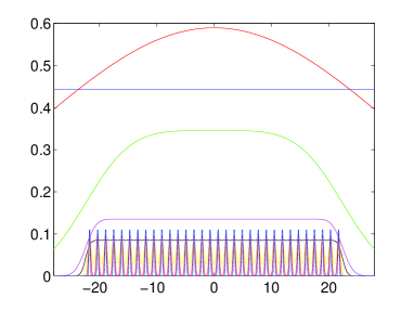
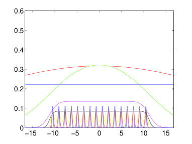
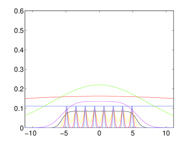
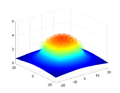
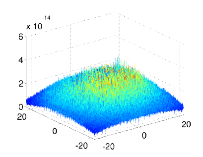
In this paper we introduce a novel grid-based $\mathit{assembled}$ tensor summation method which matches well for lattice-type and periodic molecular systems and yields enormous reduction in storage and time of calculations. The resulting canonical tensor representing the total sum of a large number of potentials contains the same number of canonical vectors as a tensor for a single potential. However, these vectors have another content: they collect the whole data from the 3D lattice by capturing the periodic shape of the total 3D potential sum (represented on the grid) onto a few 1D canonican vectors, as it is shown in Figures 3.2 and 3.5 in sections §3.1 and 3.2. This agglomeration is performed in a simple algebraic way by pointwise sums of shifted canonical vectors representing the generating function, e.g. $\frac{1}{r}$. The presented numerical calculations confirm that the difference between the total potentials obtained by an assembled tensor-product sum and by a direct canonical sum is close to machine precision, see Figure 3.4.

Thus, the adaptive global decomposition of a sum of interacting potentials can be computed with a high accuracy, and in a completely algebraic way. The resultant potential is represented simultaneously on the fine 3D Cartesian grid in the whole computational box, both in the framework of a finite lattice-type cluster, or of a supercell in a periodic setting. The corresponding rank bounds for the tensor representation of the sums of potentials are proven. Our grid-based tensor approach is beneficial in applications requiring further functional calculus with the lattice potential sums, for example, interpolation, scalar product with a function, integration or differentiation (computation of energies or forces), which can be performed on large 3D grids using tensor arithmetics of sub-linear cost [9, 31] (see Appendix). This advantage makes the tensor method promising in electronic structure calculations, for example, in computation of projections of the sum of electrostatic potentials onto some basis sets like molecular or atomic Gaussian-type orbitals.

In the case of a $L\times L\times L$ lattice cluster in a box the storage size is shown to be bounded by $O(L)$, while the summation cost is estimated by $O(NL)$. The latter can be reduced to the logarithmic scaling in the grid size, $O(L\log N)$, by using the quantized approximation of long canonical vectors (QTT approximation method [29], see Appendix). For a lattice cluster in a box both the fast multipole, FFT as well as the so-called $P^{3}M$ methods if applicable scale at least linear-logarithmic in the number of particles/nuclear charges on a lattice, $O(L^{3}\log L)$, see [40, 14].

For periodic boundary conditions, the respective lattice summations are reduced to 1D operations on short canonical vectors of size $n=N/L$, being the restriction (projection) of the global $N$-vectors onto the unit cell. Here $n$ denotes merely the number of grid points per unit cell. In this case, storage and computational costs are reduced to $O(n)$ and $O(Ln)$, respectively, while the traditional FFT-based approach scales at least cubically in $L$, $O(L^{3}\log L)$. Due to low cost of the tensor method in the limit of large lattice size $L$, the conditionally convergent sums in periodic setting can be regularized by subtraction of the constant term which can be evaluated numerically by the Richardson extrapolation on a sequence of lattice parameters $L,2L,4L$ etc. (see §3.2). Hence, in the new framework the analytic treatment of the conditionally convergent sums is no longer required.

It is worth to note that the presented tensor method is applicable to the lattice sums of rather general interaction potentials which allow an efficient local-plus-separable approximation. In particular, along with Coulombic systems, it can be applied to a wide class of commonly used interaction potentials, for example, to the Slater, Yukawa, Stokeslet, Lennard-Jones or van der Waals interactions. In all these cases the existence of low-rank grid-based tensor approximation can be proved and this approximation can be constructed numerically by analytic-algebraic methods as in the case of the Newton kernel. Our tensor approach can be extended to slightly perturbed periodic systems, for example, to the case of few vacancies in the spacial distribution of electrostatic potentials, or a small perturbation in positions of electron charges and other defects. The more detailed discussion of these issues is beyond the scope of the present paper, and is the topic of forthcoming papers.

Notice that the tensor numerical methods are now recognized as the a powerful tool for solution of multidimensional partial differential equations (PDEs) discretized by traditional grid-based schemes. Originating from the DMRG-based matrix product states decomposition in quantum physics and chemistry [44] and coupled with tensor multilinear algebra [32, 46, 20], the approach was recently developed to the new branch of numerical analysis, tensor numerical methods, providing efficient algorithms for solving multidimensional PDEs with linear complexity scaling in the dimension [45]. One of the first steps in development of tensor numerical methods was the 3D grid-based tensor-structured method for solution of the nonlinear Hartree-Fock equation [28, 12, 9, 11] based on the efficient algorithms for the grid-based calculation of the 3D convolution integral operators in 1D complexity.

The reminder of the paper is structured as follows. In Section 2 we recall the low-rank approximation to the single Newton kernel (electrostatic potential) in the canonical tensor format and direct tensor calculation of the total potential sum of arbitrarily positioned potentials in a box. Section 3 presents the main results of this paper describing the assembled low-rank tensor summation of potentials on a lattice in a bounded rectangular box, as well as in the periodic setting. The storage estimates and complexity analysis are provided. We give numerical illustrations to the structure of assembled canonical vectors and the results on accuracy and times of tensor summations over large 3D lattice. In Section 4, we prove the low QTT-rank approximation of the canonical vectors in the lattice sum of the Newton kernels that justifies the logarithmic (in the grid size $N$) storage cost of the tensor summation scheme. Section 5 concludes the paper. For the readers convenience, Appendix describes the basic notions of rank-structured tensor formats.

2 Tensor decomposition of the electrostatic potential

2.1 Grid-based canonical representation of the Newton kernel

Methods of separable approximation to the 3D Newton kernel (electrostatic potential) using the Gaussian sums have been addressed in the chemical and mathematical literature since [3] and [4, 6], respectively.

In this section, we briefly recall the grid-based method for the low-rank tensor representation of the 3D Newton kernel $\frac{1}{\|x\|}$ by its projection onto the set of piecewise constant basis functions, see [28] for more details. Based on the results in [19, 23, 1], this approximation can be proven to converge almost exponentially in the rank parameter. For the readers convenience, we now recall the main ingredients of this tensor approximation scheme [1].

In the computational domain $\Omega=[-b/2,b/2]^{3}$, let us introduce the uniform $n\times n\times n$ rectangular Cartesian grid $\Omega_{n}$ with the mesh size $h=b/n$. Let $\{\psi_{\textbf{i}}\}$ be a set of tensor-product piecewise constant basis functions, $\psi_{\textbf{i}}(\textbf{x})=\prod_{\ell=1}^{d}\psi_{i_{\ell}}^{(\ell)}(x_{\ell})$ for the $3$-tuple index $\textbf{i}=(i_{1},i_{2},i_{3})$, $i_{\ell}\in I=\left\{1,...,n\right\}$, $\ell=1,\,2,\,3$. The Newton kernel can be discretized by its projection onto the basis set $\{\psi_{\textbf{i}}\}$ in the form of a third order tensor of size $n\times n\times n$, given point-wise as

$$\mathbf{P}:=\left[p_{\textbf{i}}\right]\in\mathbb{R}^{n\times n\times n},\quad p_{\textbf{i}}=\int_{\mathbb{R}^{3}}\frac{\psi_{\textbf{i}}(\textbf{x})}{\|\mathbf{x}\|}\,\,\mathrm{d}\textbf{x}.$$ (2.1)

The low-rank canonical decomposition of the 3D tensor $\mathbf{P}$ is based on using exponentially convergent $\operatorname*{sinc}$-quadratures for approximation of the Laplace-Gauss transform to the Newton kernel,

$$\frac{1}{\|\mathbf{x}\|} =\frac{1}{\sqrt{\pi}}\int_{\mathbb{R}}e^{-t^{2}\|\mathbf{x}\|^{2}}\,\mathrm{d}t=\frac{1}{\sqrt{\pi}}\int_{\mathbb{R}}\prod_{\ell=1}^{3}e^{-t^{2}(x_{\ell})^{2}}\,\mathrm{d}t,\quad\|\mathbf{x}\|>0.$$ (2.2)

Following [23, 1], for any fixed $x\in\mathbb{R}^{3}$, we apply the $\operatorname*{sinc}$-quadrature approximation

$$\frac{1}{\|\mathbf{x}\|}=\frac{1}{\sqrt{\pi}}\int_{\mathbb{R}}e^{-t^{2}\|\mathbf{x}\|^{2}}\,\mathrm{d}t\approx\sum_{k=-M}^{M}g_{k}e^{-t_{k}^{2}\|\mathbf{x}\|^{2}}\quad\mbox{for}\quad\|\mathbf{x}\|>0,$$ (2.3)

where the quadrature points and weights are given by

$$t_{k}=k\mathfrak{h}_{M},\ g_{k}=\mathfrak{h}_{M},\ \mathfrak{h}_{M}=C_{0}\log(M)/M,\ C_{0}>0.$$ (2.4)

Under the assumption $0<a\leq\|\mathbf{x}\|\leq A<\infty$ this quadrature provides the exponential convergence rate in $M$,

$$\left|\frac{1}{\|\mathbf{x}\|}-\sum_{k=-M}^{M}g_{k}e^{-t_{k}^{2}\|\mathbf{x}\|^{2}}\right|\leq\frac{C}{a}\,\displaystyle e^{-\beta\sqrt{M}},\quad\text{with some}\ C,\beta>0.$$

Combining (2.1) and (2.3), and taking into account the separability of the Gaussian and basis functions, we obtain the separable approximation to each entry of the tensor $\mathbf{P}$,

$$p_{\textbf{i}}\approx\sum_{k=-M}^{M}g_{k}\int_{\mathbb{R}^{3}}\psi_{\textbf{i}}(\textbf{x})e^{-t_{k}^{2}\|\mathbf{x}\|^{2}}\mathrm{d}\textbf{x}=\sum_{k=-M}^{M}g_{k}\prod_{\ell=1}^{3}\int_{\mathbb{R}}\psi^{(\ell)}_{i_{\ell}}(x_{\ell})e^{-t_{k}^{2}x^{2}_{\ell}}\mathrm{d}x_{\ell}.$$ (2.5)

Define the vector

$$\textbf{b}^{(\ell)}(t_{k})=\{b^{(\ell)}_{i_{\ell}}(t_{k})\}\in\mathbb{R}^{n_{\ell}}\quad\text{with }\quad b^{(\ell)}_{i_{\ell}}(t_{k})=\int_{\mathbb{R}}\psi^{(\ell)}_{i_{\ell}}(x_{\ell})e^{-t_{k}^{2}x^{2}_{\ell}}\mathrm{d}x_{\ell},$$ (2.6)

then the $3$rd order tensor $\mathbf{P}$ can be approximated by the rank-$R$ ($R=2M+1$) canonical representation

$$\mathbf{P}\approx\mathbf{P}_{R}=\sum_{k=-M}^{M}g_{k}\bigotimes_{\ell=1}^{3}\textbf{b}^{(\ell)}(t_{k})\in\mathbb{R}^{n\times n\times n},\quad g_{k},\,t_{k}\in\mathbb{R},$$

where $R=2M+1$ and $M$ is chosen in such a way that in the max-norm

$$\|\mathbf{P}-\mathbf{P}_{R}\|\leq\varepsilon\|\mathbf{P}\|,$$

where $\varepsilon>0$ is the given tolerance. This construction defines the rank-$R$ ($R\leq M+1$) canonical tensor

$${\bf P}_{R}=\sum\limits_{q=1}^{R}{\bf p}^{(1)}_{q}\otimes{\bf p}^{(2)}_{q}\otimes{\bf p}^{(3)}_{q}\in\mathbb{R}^{n\times n\times n},$$ (2.7)

with canonical vectors obtained by renumbering $q=k+M+1$, ${\bf p}^{(\ell)}_{q}=g_{k}\textbf{b}^{(\ell)}(t_{k})\in\mathbb{R}^{n}$, $\ell=1,\,2,\,3$. This tensor approximates the discretized 3D symmetric Newton kernel $\frac{1}{\|x\|}$ ($x\in\Omega$), centered at the origin, such that ${\bf p}^{(1)}_{q}={\bf p}^{(2)}_{q}={\bf p}^{(3)}_{q}$ ($q=1,...,R$).

Figure 2.1: Several vectors of the canonical tensor representation for a single Newton kernel along $x$-axis from a set $\{{\bf p}^{(1)}_{q}\}_{q=1}^{R}$.

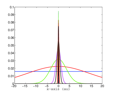
Figure 2.1 displays several vectors of the canonical tensor representation for a single Newton kernel along $x$-axis from a set $\{P^{(1)}_{q}\}_{q=1}^{R}$. Symmetry of the tensor ${\bf P}_{R}$ implies that the vectors ${\bf p}^{(2)}_{q}$ and ${\bf p}^{(3)}_{q}$ corresponding to $y$ and $z$-axes, respectively, are of the same shape as ${\bf p}^{(1)}_{q}$. It is clearly seen that there are canonical vectors representing the long-, intermediate- and short-range contributions to the total electrostatic potential. This interesting feature will be also recognized for the low-rank lattice sum of potentials (see Section 3).

Table 2.1 presents CPU times for generating a canonical rank-$R$ tensor approximation of the Newton kernel over $n\times n\times n$ 3D Cartesian grid, corresponding to Matlab implementation on a terminal of the 8 AMD Opteron Dual-Core processor. We observe a logarithmic scaling of the canonical rank $R$ in the grid size. The compression rate denotes the ratio $n^{3}/(nR)$.

grid size $n^{3}$	$8192^{3}$	$16384^{3}$	$32768^{3}$	$65536^{3}$	$131072^{3}$
Time (sec.)	$6$	$16$	$61$	$241$	$1000$
Canonical rank $R$	$34$	$37$	$39$	$41$	$43$
Compression rate	$2\cdot 10^{6}$	$7\cdot 10^{6}$	$2\cdot 10^{7}$	$1\cdot 10^{8}$	$4\cdot 10^{8}$

Table 2.1: CPU times (Matlab) to compute canonical vectors of ${\bf P}_{R}$ for the Newton kernel in a box with tolerance $\varepsilon=10^{-7}$.

Notice that the low-rank canonical decomposition of the tensor ${\bf P}$ is the problem independent task, hence the respective canonical vectors can be precomputed at once on very large 3D $n\times n\times n$ grid, and then stored for the multiple use. The storage size is bounded by $O(Rn)$.

The direct tensor summation method described below is based on the use of low-rank canonical representation to the single Newton kernel ${\bf P}_{R}$ in the bounding box, translated and restricted according to coordinates of the potentials in a box.

2.2 Direct tensor summation of electrostatic interactions

Here, we recall tensor summation of the electrostatic potentials for a non-lattice structure, that is for a (rather small) number of an arbitrarily distributed sources [10, 11]. As the basic example in electronic structure calculations, we consider the nuclear potential operator describing the Coulombic interaction of electrons with the nuclei in a molecular system in a box or in a (cubic) unit cell. It is defined by the function $v_{c}(x)$ in the scaled unit cell $\Omega=[-b/2,b/2]^{3}$,

$$v_{c}(x)=\sum_{\nu=1}^{M_{0}}\frac{Z_{\nu}}{\|{x}-a_{\nu}\|},\quad Z_{\nu}>0,\;\;x,a_{\nu}\in\Omega\subset\mathbb{R}^{3},$$ (2.8)

where $M_{0}$ is the number of nuclei in $\Omega$, and $a_{\nu}$, $Z_{\nu}$, represent their coordinates and charges, respectively.

We begin with approximating the non-shifted 3D Newton kernel $\frac{1}{\|x\|}$ on the auxiliary extended box $\widetilde{\Omega}=[-b,b]^{3}$, by its projection onto the basis set $\{\psi_{\textbf{i}}\}$ of piecewise constant functions defined on the uniform $2n\times 2n\times 2n$ tensor grid $\Omega_{2n}$ with the mesh size $h$, as described in Section 2.1. This defines the ”master“ rank-$R$ canonical tensor as above

$$\widetilde{\bf P}_{R}=\sum\limits_{q=1}^{R}{\bf p}^{(1)}_{q}\otimes{\bf p}^{(2)}_{q}\otimes{\bf p}^{(3)}_{q}\in\mathbb{R}^{2n\times 2n\times 2n}.$$ (2.9)

For ease of exposition, we assume that each nuclei coordinate $a_{\nu}$ is located exactly at a grid-point $a_{\nu}=(i_{\nu}h-b/2,j_{\nu}h-b/2,k_{\nu}h-b/2)$, with some $1\leq i_{\nu},j_{\nu},k_{\nu}\leq n$. Now we are able to introduce the rank-$1$ windowing operator ${\cal W}_{\nu}={\cal W}_{\nu}^{(1)}\otimes{\cal W}_{\nu}^{(2)}\otimes{\cal W}_{\nu}^{(3)}$ for $\nu=1,...,M_{0}$ by

$${\cal W}_{\nu}\widetilde{\bf P}_{R}:=\widetilde{\bf P}_{R}(i_{\nu}+n/2:i_{\nu}+3/2n;j_{\nu}+n/2:j_{\nu}+3/2n;k_{\nu}+n/2:k_{\nu}+3/2n)\in\mathbb{R}^{n\times n\times n},$$ (2.10)

With this notation, the total electrostatic potentials $v_{c}(x)$ in the computational box $\Omega$ is approximately represented by a direct canonical tensor sum

$$\begin{split}{\bf P}_{c}&=\sum_{\nu=1}^{M_{0}}Z_{\nu}{\cal W}_{\nu}\widetilde{\bf P}_{R}\\ &=\sum_{\nu=1}^{M_{0}}Z_{\nu}\sum\limits_{q=1}^{R}{\cal W}_{\nu}^{(1)}{\bf p}^{(1)}_{q}\otimes{\cal W}_{\nu}^{(2)}{\bf p}^{(2)}_{q}\otimes{\cal W}_{\nu}^{(3)}{\bf p}^{(3)}_{q}\in\mathbb{R}^{n\times n\times n},\end{split}$$ (2.11)

with the rank bound

$$rank({\bf P}_{c})\leq M_{0}R,$$

where every rank-$R$ canonical tensor ${\cal W}_{\nu}\widetilde{\bf P}_{R}\in\mathbb{R}^{n\times n\times n}$ is thought as a sub-tensor of the master tensor $\widetilde{\bf P}_{R}\in\mathbb{R}^{2n\times 2n\times 2n}$ obtained by its shifting and restriction (windowing) onto the $n\times n\times n$ grid in the box $\Omega$, $\Omega_{n}\subset\Omega_{2n}$. Here a shift from the origin is specified according to the coordinates of the corresponding nuclei, $a_{\nu}$, counted in the $h$-units.

For example, the electrostatic potential centered at the origin, i.e. with $a_{\nu}=0$, corresponds to the restriction of $\widetilde{\bf P}_{R}$ onto the initial computational box $\Omega_{n}$, i.e. to the index set (assume that $n$ is even)

$$\{[n/2+i]\times[n/2+j]\times[n/2+k]\},\quad i,j,k\in\{1,...,n\}.$$

Remark 2.1

The rank estimate (2.11) for the sum of arbitrarily positioned electrostatic potentials in a box (unit cell), $R_{c}=rank({\bf P}_{c})\leq M_{0}R$, is usually too pessimistic. Our numerical tests for moderate size molecules indicate that the rank of the $(M_{0}R)$-term canonical sum in (2.11) can be considerably reduced. This rank optimization can be implemented by the multigrid version of the canonical rank reduction algorithm, canonical-Tucker-canonical [31]. The resultant canonical tensor will be denoted by $\widehat{\bf P}_{c}$.

The proposed grid-based representation of the exact sum of electrostatic potentials $v_{c}(x)$ in a form of a tensor in a canonical format enables its easy projection to some separable basis set, like GTO-type atomic orbital basis often used in quantum chemical computations. The following example illustrates calculation of the nuclear potential operator matrix in tensor format for molecules [10, 11]. We show that the projection of a sum of electrostatic potentials of atoms onto a given set of basis functions is reduced to a combination of 1D Hadamard and scalar products (cf. (6.2)-(6.3) in Appendix).

Example 2.2

[10, 11] Let us discuss the tensor-structured calculation of the nuclear potential operator in a molecule. Given the set of continuous basis functions,

$$\{g_{\mu}(x)\},\quad\mu=1,...,N_{b},$$ (2.12)

then each of them can be discretized by a third order tensor,

$${\bf G}_{\mu}=\left[g_{\mu}(x_{1}(i),x_{2}(j),x_{3}(k))\right]_{i,j,k=1}^{n}\in\mathbb{R}^{n\times n\times n},$$

obtained by sampling of $g_{\mu}(x)$ at the midpoints $(x_{1}(i),x_{2}(j),x_{3}(k))$ of the grid-cells indexed by $(i,j,k)$. Suppose, for simplicity, that it is a rank-$1$ canonical tensor, $rank({\bf G}_{\mu})=1$, i.e.

$${\bf G}_{\mu}=G_{\mu}^{(1)}\otimes G_{\mu}^{(2)}\otimes G_{\mu}^{(3)}\in\mathbb{R}^{n\times n\times n},$$

with the canonical vectors $G_{\mu}^{(\ell)}\in\mathbb{R}^{n}$, associated with mode $\ell=1,2,3$.

A sum of potentials in a box, $v_{c}(x)$ (2.8), is represented in the given basis set (2.12) by a matrix $V_{c}=\{{v}_{km}\}\in\mathbb{R}^{N_{b}\times N_{b}}$, whose entries are calculated (approximated) by the simple tensor operation, see [10, 11],

$${v}_{km}=\int_{\mathbb{R}^{3}}v_{c}(x){g}_{k}(x){g}_{m}(x)dx\approx\langle{\bf G}_{k}\odot{\bf G}_{m},{\bf P}_{c}\rangle,\quad 1\leq k,m\leq N_{b}.$$ (2.13)

Here ${\bf P}_{c}$ is a sum of shifted/windowed canonical tensors (2.11) representing the total electrostatic potential of atoms in a molecule, and

$${\bf G}_{k}\odot{\bf G}_{m}=(G_{k}^{(1)}\odot G_{m}^{(1)})\otimes(G_{k}^{(2)}\odot G_{m}^{(2)})\otimes(G_{k}^{(3)}\odot G_{m}^{(3)})$$

denotes the Hadamard (entrywise) product of tensors representing the basis functions (6.3), which is reduced to 1D products. The scalar product $\langle\cdot,\cdot\rangle$ in (2.13) is also reduced to 1D scalar products (6.2) due to separation of variables.

To conclude this section, we notice that the approximation error $\varepsilon>0$ caused by a separable representation of the nuclear potential is controlled by the rank parameter $R_{c}=rank({\bf P}_{c})\approx C\,R$, where $C$ depends on the number of nuclei $M_{0}$. Now letting $rank({\bf G}_{m})=1$ implies that each matrix element is to be computed with linear complexity in $n$, $O(R\,n)$. The exponential convergence of the canonical approximation in the rank parameter $R$ allows us the optimal choice $R=O(|\log\varepsilon|)$ adjusting the overall complexity bound $O(|\log\varepsilon|\,n)$, independent on $M_{0}$.

3 Lattice potential sums by assembled canonical tensors

In the numerical treatment of extended systems the 3D summation over $L^{3}$ cells in the limit of large $L$ is considered as a hard computational task both in a bounded and in a periodic setting. The commonly used methods, known in the literature as the Ewald summation algorithms [18], are based on a certain specific local-global decomposition of the Newton kernel (see [41, 25, 14])

$$\frac{1}{r}=\frac{\tau(r)}{r}+\frac{1-\tau(r)}{r},$$

where the traditional choice of the cutoff function $\tau$ is the complementary error function

$$\tau(r)=\operatorname{erfc}(r):=\frac{2}{\sqrt{\pi}}\int_{r}^{\infty}\exp(-t^{2})dt.$$

In this paper, we introduce a new grid-based approach to the problem of lattice summation of electrostatic potentials in a box/supercell based on the fast agglomerated tensor sums. The resulting total potential on the lattice is represented in a form of a low-rank canonical tensor. The main ingredients are the separable canonical tensor approximation of the Newton kernel and fast rank-structured tensor arithmetics. The proposed tensor method is not limited to a special case of Newton kernel $\frac{1}{\|x\|}$, and can be applied to a general class of shift-invariant well separable generating potentials.

3.1 Assembled lattice sums in a box

In this section, we present the efficient scheme for fast agglomerated tensor summation of electrostatic potentials for a lattice in a box. Given the potential sum $v_{c}$ in the unit reference cell $\Omega=[-b/2,b/2]^{d}$, $d=3$, of size $b\times b\times b$, we consider an interaction potential in a bounded box

$$\Omega_{L}=B_{1}\times B_{2}\times B_{3},$$

consisting of a union of $L_{1}\times L_{2}\times L_{3}$ unit cells $\Omega_{\bf k}$, obtained by a shift of $\Omega$ that is a multiple of $b$ in each variable, and specified by the lattice vector $b{\bf k}$, ${\bf k}=(k_{1},k_{2},k_{3})\in\mathbb{Z}^{d}$, $0\leq k_{\ell}\leq L_{\ell}-1$ for $L_{\ell}\in\mathbb{N}$, ($\ell=1,2,3$). Here $B_{\ell}=[-b/2,b/2+(L_{\ell}-1)b]$ , such that the case $L_{\ell}=1$ corresponds to one-layer systems in the variable $x_{\ell}$. Recall that by the construction $b=nh$, where $h>0$ is the mesh-size (same for all spacial variables).

In the case of an extended system in a box the summation problem for the total potential $v_{c_{L}}(x)$ is formulated in the rectangular volume $\Omega_{L}=\bigcup_{k_{1},k_{2},k_{3}=1}^{L}\Omega_{\bf k}$, where for ease of exposition we consider a lattice of equal sizes $L_{1}=L_{2}=L_{3}=L$. In general, the volume box for calculations is larger than $\Omega_{L}$, by a distance of several $\Omega$ (see Figures 3.1 and 3.2). On each $\Omega_{\bf k}\subset\Omega_{L}$, the potential sum of interest, $v_{\bf k}(x)=(v_{c_{L}})_{|\Omega_{\bf k}}$, is obtained by summation over all unit cells in $\Omega_{L}$,

$$v_{\bf k}(x)=\sum_{\nu=1}^{M_{0}}\sum\limits_{k_{1},k_{2},k_{3}=0}^{L-1}\frac{Z_{\nu}}{\|{x}-a_{\nu}(k_{1},k_{2},k_{3})\|},\quad x\in\Omega_{\bf k},$$ (3.1)

where $a_{\nu}(k_{1},k_{2},k_{3})=a_{\nu}+b{\bf k}$. This calculation is performed at each of $L^{3}$ elementary cells $\Omega_{\bf k}\subset\Omega_{L}$, which usually presupposes substantial numerical costs for large $L$. In the presented approach these costs are essentially reduced, as it is described further.

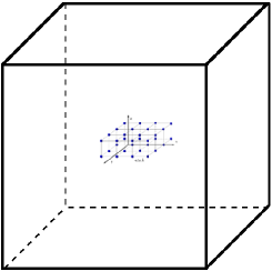
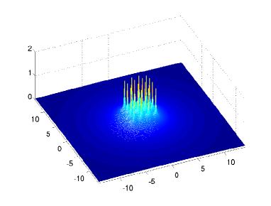
Figure 3.1 shows the example of a computational box with a 3D lattice-type molecular structure of $4\times 4\times 2$ atoms and the calculated lattice sum of electrostatic potentials.

Figure 3.1: Example of $4\times 4\times 2$ lattice compound in a computational box and calculated potential sum.

Let $\Omega_{N_{L}}$ be the $N_{L}\times N_{L}\times N_{L}$ uniform grid on $\Omega_{L}$ with the same mesh-size $h$ as above, and introduce the corresponding space of piecewise constant basis functions of the dimension $N_{L}^{3}$. In this construction we have

$$N_{L}=n+n(L-1)=Ln.$$ (3.2)

Similar to (2.9), we employ the rank-$R$ ”master“ tensor defined on the auxiliary box $\widetilde{\Omega}_{L}$ by scaling ${\Omega}_{L}$ with factor $2$.

$$\widetilde{\bf P}_{{L},R}=\sum\limits_{q=1}^{R}{\bf p}^{(1)}_{q}\otimes{\bf p}^{(2)}_{q}\otimes{\bf p}^{(3)}_{q}\in\mathbb{R}^{2N_{L}\times 2N_{L}\times 2N_{L}},$$

and let ${\cal W}_{\nu(k_{i})}$, $i=1,2,3$, be the directional windowing operators associated with the lattice vector ${\bf k}$. In the next theorem we prove the storage and numerical costs for the lattice sum of single potentials, each represented by a canonical rank-$R$ tensor, which corresponds to the choice $M_{0}=1$, and $a_{1}=0$ in (3.1). In this case the windowing operator ${\cal W}={\cal W}_{({\bf k})}$ specifies the shift by the lattice vector $b{\bf k}$.

Theorem 3.1

The projected tensor of the interaction potential $v_{c_{L}}(x)$, $x\in\Omega_{L}$, representing the full lattice sum over $L^{3}$ charges can be presented by the canonical tensor ${\bf P}_{c_{L}}$ with the rank $R$,

$${\bf P}_{c_{L}}=\sum\limits_{q=1}^{R}(\sum\limits_{k_{1}=0}^{L-1}{\cal W}_{({k_{1}})}{\bf p}^{(1)}_{q})\otimes(\sum\limits_{k_{2}=0}^{L-1}{\cal W}_{({k_{2}})}{\bf p}^{(2)}_{q})\otimes(\sum\limits_{k_{3}=0}^{L-1}{\cal W}_{({k_{3}})}{\bf p}^{(3)}_{q}).$$ (3.3)

The numerical cost and storage size are estimated by $O(RLN_{L})$ and $O(RN_{L})$, respectively, where $N_{L}$ is the univariate grid size as in (3.2).

Proof. For the moment, we fix index $\nu=1$ in (3.1) and consider only the second sum defined on the complete domain $\Omega_{L}$,

$${v}_{c_{L}}(x)=\sum\limits_{k_{1},k_{2},k_{3}=0}^{L-1}\frac{Z}{\|{x}-b{\bf k}\|},\quad x\in\Omega_{L}.$$ (3.4)

Then the projected tensor representation of ${v}_{c_{L}}(x)$ takes the form (omitting factor $Z$)

$${\bf P}_{c_{L}}=\sum\limits_{k_{1},k_{2},k_{3}=0}^{L-1}{\cal W}_{\nu({\bf k})}{\bf P}_{{L},R}=\sum\limits_{k_{1},k_{2},k_{3}=0}^{L-1}\sum\limits_{q=1}^{R}{\cal W}_{({\bf k})}({\bf p}^{(1)}_{q}\otimes{\bf p}^{(2)}_{q}\otimes{\bf p}^{(3)}_{q})\in\mathbb{R}^{N_{L}\times N_{L}\times N_{L}},$$

where the 3D shift vector is defined by ${\bf k}\in\mathbb{Z}^{L\times L\times L}$. Taking into account the separable representation of the $\Omega_{L}$-windowing operator (tracing onto $N_{L}\times N_{L}\times N_{L}$ window),

$${\cal W}_{({\bf k})}={\cal W}_{(k_{1})}^{(1)}\otimes{\cal W}_{(k_{2})}^{(2)}\otimes{\cal W}_{(k_{3})}^{(3)},$$

we reduce the above summation to

$${\bf P}_{c_{L}}=\sum\limits_{q=1}^{R}\sum\limits_{k_{1},k_{2},k_{3}=0}^{L-1}{\cal W}_{({k_{1}})}{\bf p}^{(1)}_{q}\otimes{\cal W}_{({k_{2}})}{\bf p}^{(2)}_{q}\otimes{\cal W}_{({k_{3}})}{\bf p}^{(3)}_{q}.$$ (3.5)

To reduce the large sum over the full 3D lattice, we use the following property of a sum of canonical tensors with equal ranks $R$ and with two coinciding factor matrices: the concatenation (6.4) in the third mode $\ell$ can be reduced to point-wise summation of respective canonical vectors,

$$C^{(\ell)}=[{\bf a}_{1}^{(\ell)}+{\bf b}_{1}^{(\ell)},\ldots,{\bf a}_{R_{a}}^{(\ell)}+{\bf b}_{R_{b}}^{(\ell)}],$$ (3.6)

thus preserving the same rank parameter $R$ for the resulting sum. Notice that for each fixed $q$ the inner sum in (3.5) satisfies the above property. Repeatedly using this property to a large number of canonical tensors, the 3D-sum (3.5) can be simplified to a rank-$R$ tensor obtained by 1D summations only,

$$\begin{split}{\bf P}_{c_{L}}&=\sum\limits_{q=1}^{R}(\sum\limits_{k_{1}=0}^{L-1}{\cal W}_{({k_{1}})}{\bf p}^{(1)}_{q})\otimes(\sum\limits_{k_{2},k_{3}=0}^{L-1}{\cal W}_{({k_{2}})}{\bf p}^{(2)}_{q}\otimes{\cal W}_{({k_{3}})}{\bf p}^{(3)}_{q})\\ &=\sum\limits_{q=1}^{R}(\sum\limits_{k_{1}=0}^{L-1}{\cal W}_{({k_{1}})}{\bf p}^{(1)}_{q})\otimes(\sum\limits_{k_{2}=0}^{L-1}{\cal W}_{({k_{2}})}{\bf p}^{(2)}_{q})\otimes(\sum\limits_{k_{3}=0}^{L-1}{\cal W}_{({k_{3}})}{\bf p}^{(3)}_{q}).\end{split}$$

The numerical cost can be estimated by taking into account the standard properties of canonical tensors.   

Figure 3.2: Agglomerated canonical vectors for a sum of electrostatic potentials for a cluster of $32\times 16\times 8$ Hydrogen atoms in a rectangular box of size $\sim 55.4\times 33.6\times 22.4$ $au^{3}$. Top left-right: vectors along $x$- and $y$-axes, respectively; bottom left: vectors along $z$-axis. Right bottom: the resulting sum of $4096$ nuclei potentials at cross-section with $z=0.83$ au.

Remark 3.2

For the general case $M_{0}>1$, the weighted summation over $M_{0}$ charges leads to the low-rank tensor representation,

$${\bf P}_{c_{L}}=\sum\limits_{\nu=1}^{M_{0}}Z_{\nu}\sum\limits_{q=1}^{R}(\sum\limits_{k_{1}=0}^{L-1}{\cal W}_{\nu({k_{1}})}{\bf p}^{(1)}_{q})\otimes(\sum\limits_{k_{2}=0}^{L-1}{\cal W}_{\nu({k_{2}})}{\bf p}^{(2)}_{q})\otimes(\sum\limits_{k_{3}=0}^{L-1}{\cal W}_{\nu({k_{3}})}{\bf p}^{(3)}_{q}).$$ (3.7)

Remark 3.3

The previous construction applies to the uniformly spaced positions of charges. However, our tensor summation method remains valid for a non-equidistant $L\times L\times L$ tensor lattice.

Figure 3.2 illustrates the shape of canonical vectors for the $32\times 16\times 8$ lattice sum in a box (summation of $4096$ potentials). Here the canonical rank $R=25$, and $\varepsilon=10^{-6}$. It demonstrates how the assembled vectors composing the tensor lattice sum incorporate simultaneously the canonical vectors of shifted Newton kernels. It can be seen that separate canonical vectors capture the local, intermediate and long-range contributions to the total sum.

Figure 3.3: CPU times ($\log$ scaling) for calculating the sum of Coulomb potentials over 3D $L\times L\times L$ lattice by using direct canonical tensor summation (blue line) and assembled lattice summation (red line).

$L$	$2$	$4$	$8$	$16$	$32$	$64$	$128$
Times for $L\times L\times 1$	$0.003$	$0.004$	$0.0073$	$0.025$	$0.128$	$0.65$	$2.96$
Times for $L\times L\times L$	$0.003$	$0.005$	$0.0098$	$0.039$	$0.19$	$0.88$	$4.01$
$L^{3}$	$8$	$64$	$512$	$4096$	$32768$	$262144$	$2097152$

Table 3.1: Times (sec) vs. $L$ for the assembled calculation of the lattice potential ${\bf P}_{c_{L}}$ for the clusters $L\times L\times 1$ and $L\times L\times L$. The last line shows the total number of cells (here Hydrogen atoms) for the clusters of type $L\times L\times L$.

Figure 3.4: Left: The electrostatic potential of the cluster of $16\times 16\times 2$ Hydrogen atoms in a box (512 atoms). Right: the absolute error of the assembled tensor sum on this cluster by (3.3) with respect to the direct tensor summation (2.11).

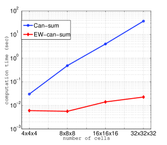
The canonical tensor representation (3.3) reduces dramatically the numerical costs and storage consumptions. Figure 3.3 compares the direct and assembled tensor summation methods (grid-size of a unit cell, $n=256$). Contrary to the direct canonical summation of the nuclear potentials on a 3D lattice that scales at least linearly in the size of the cubic lattice, $N_{L}L^{3}$ (blue line), the CPU time for directionally agglomerated canonical summation in a box via (3.3) scales as $N_{L}L$ (red line).

Table 3.1 illustrates complexity scaling $O(N_{L}L)$ for tensor lattice summation in a box of size $L\times L\times 1$ and $L\times L\times L$. We observe the $L^{2}$ scaling which confirms our theoretical estimates.

Figure 3.4 compares the tensor sum obtained by the assembled canonical vectors with the results of direct tensor sum for same configuration. The absolute difference of the corresponding sums for a cluster of $16\times 16\times 2$ cells (here a cluster of 512 Hydrogen atoms) is close to machine accuracy $\sim 10^{-14}$.

3.2 Assembled tensor sums in a periodic setting

In the periodic case we introduce the periodic cell ${\cal R}=b\mathbb{Z}^{d}$, $d=1,2,3$, and consider a 3D $T$-periodic supercell of size $T\times T\times T$, with $T=bL$. The total electrostatic potential in $\Omega_{L}$ is obtained by the respective summation over the supercell $\Omega_{L}$ for possibly large $L$. Then the electrostatic potential in any of $T$-periods is obtained by replication of the respective data from $\Omega_{L}$.

The potential sum $v_{c_{L}}(x)$ is designated at each elementary unit-cell in $\Omega_{L}$ by the same value (${\bf k}$-translation invariant). Consider the case $d=3$. Supposing for simplicity that $L$ is odd, $L=2p+1$, the reference value of $v_{c_{L}}(x)$ will be computed at the central cell $\Omega_{0}$, indexed by $(p+1,p+1,p+1)$, by summation over all the contributions from $L^{3}$ elementary sub-cells in $\Omega_{L}$,

$$v_{0}(x)=\sum_{\nu=1}^{M_{0}}\sum\limits_{k_{1},k_{2},k_{3}=1}^{L}\frac{Z_{\nu}}{\|{x}-a_{\nu}(k_{1},k_{2},k_{3})\|},\quad x\in\Omega_{0}.$$ (3.8)

Now the projected tensor sum can be computed by a simple modification of (3.7).

Lemma 3.4

The projected tensor of $v_{\Omega_{L}}$ for the full sum over $M_{0}$ charges can be presented by rank-$(M_{0}R)$ canonical tensor. The computational cost is estimated by $O(M_{0}RnL)$, while the storage size is bounded by $O(M_{0}Rn)$.

Proof. We fix index $\nu=1$ in (3.8) and chose the central cell $\Omega_{0}$ as above to obtain

$$v_{\Omega_{L}}(x)=\sum\limits_{k_{1},k_{2},k_{3}=1}^{L}\frac{Z_{\nu}}{\|{x}-a_{\nu}(k_{1},k_{2},k_{3})\|},\quad x\in\Omega_{0},$$ (3.9)

for the local lattice sum on the index set $n\times n\times n$, and

$${\bf P}_{\Omega_{0}}=Z_{\nu}\sum\limits_{k_{1},k_{2},k_{3}=1}^{L}{\cal W}_{\nu({\bf k})}{\bf P}_{\Omega_{0}}=Z_{\nu}\sum\limits_{k_{1},k_{2},k_{3}=1}^{L}\sum\limits_{q=1}^{R_{\cal N}}{\cal W}_{\nu({\bf k})}{\bf p}^{(1)}_{q}\otimes{\bf p}^{(2)}_{q}\otimes{\bf p}^{(3)}_{q}\in\mathbb{R}^{n\times n\times n},$$

for the corresponding local projected tensor of small size $n\times n\times n$. Here we adapt the $\Omega$-windowing operator, ${\cal W}_{\nu({\bf k})}={\cal W}_{\nu(k_{1})}^{(1)}\otimes{\cal W}_{\nu(k_{2})}^{(2)}\otimes{\cal W}_{\nu(k_{3})}^{(3)},$ that projects onto the small $n\times n\times n$ unit cell by shifting on the lattice vector ${\bf k}=(k_{1},k_{2},k_{3})$. Now the canonical representation follows by the arguments as in the proof of Theorem 3.1, with the similar complexity analysis.   

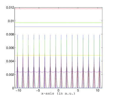
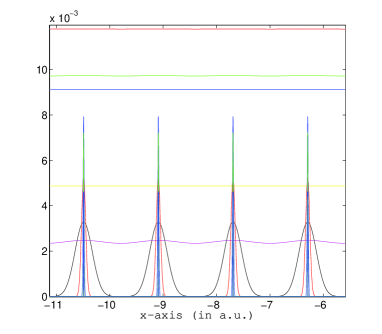
Figure 3.5 shows the assembled canonical vectors for a lattice structure in a periodic setting.

Figure 3.5: Periodic canonical vectors in the $L\times 1\times 1$ lattice sum, $L=16$ (left); Zooming of four periods (right).

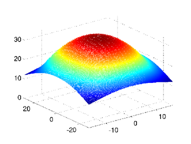
Recall that in the limit of large $L$ the lattice sum ${\bf P}_{c_{L}}$ of the Newton kernels is known to converge only conditionally. The same is true for a sum in a box. The maximum norm increases as $C_{1}\log L$, $C_{2}L$ and $C_{3}L^{2}$ for 1D, 2D and 3D sums, respectively (see Figure3.6). This issue is of special significance in the periodic setting, dealing with the limiting case $L\to\infty$. To approach the limiting case, we compute a ${\bf P}_{c_{L}}$ on a sequence of large parameters $L,2L,4L$ etc. and then apply the Richardson extrapolation as described in the following. As result, we obtain the regularized tensor $\widehat{p}_{L}$ restricted to the reference unit cell $\Omega_{0}$.

Figure 3.6 presents the value $p_{0}$ of the potential sum at the center of a bounded box vs. $L$, for $L\times 1\times 1$, $L\times L\times 1$ and $L\times L\times L$ lattice sums, where $L=2,4,8,...,128$. The predicted asymptotic behaviour in $L$ is easily seen.

Figure 3.6: Potential sum $p_{L}$ at the center of the supercell vs. $L$ for $L\times 1\times 1$, $L\times L\times 1$ and $L\times L\times L$ lattice sums.

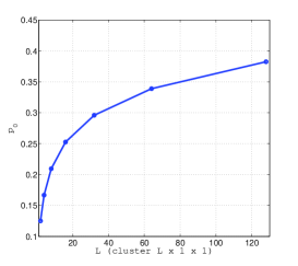
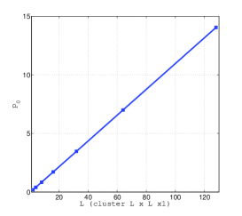
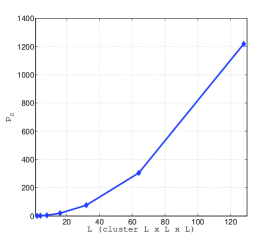
In the traditional Ewald-type summation techniques the regularization of lattice sums is implemented by subtraction of the analytically precomputed constants describing the asymptotic behaviour in $L$. In our tensor summation method this problem is solved by algebraic approach by using the Richardson extrapolation techniques applied on a sequence of supercells with increasing size $L$, $2L$, $4L$, etc. Denoting the target value of the potential by $p_{L}$, the extrapolation formulas for the linear and quadratic behaviour take form

$$\widehat{p}_{L}:=2p_{L}-p_{2L},\quad\mbox{and}\quad\widehat{p}_{L}:=(4p_{L}-p_{2L})/3,$$

respectively. The effect of Richardson extrapolation is illustrated in Figure 3.7.

Figure 3.7: Regularized potential sum $\widehat{p}_{L}$ vs. $m$ with $L=2^{m}$, for $L\times L\times 1$ (left), and $L\times L\times L$ lattice sums (right).

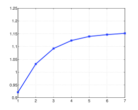
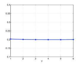
Figure 3.7 indicates that the potential sum computed at the same point as for the previous example (in the case of $L\times L\times 1$ and $L\times L\times L$ lattices) converges to the limiting values of $\widehat{p}_{L}$ after application the Richardson extrapolation (regularized sum).

4 QTT ranks of the assembled canonical vectors in the lattice sum

Agglomerated canonical vectors in the rank-$R$ tensor representation (3.3) are defined over large uniform grid of size $N_{L}$. Hence numerical cost for evaluation of each of these $3R$ vectors scales as $O(N_{L}L)$, which might become too expensive for large $L$ (recall that $N_{L}=nL$ scales linear in $L$). Using quantics-TT (QTT) approximation [29], this cost can be reduced to the logarithmic scale in $N_{L}$, while the storage need will become $O(\log N_{L})$ only.

Our QTT-rank estimates are based on three main ingredients: the global canonical tensor representation of $1/\|x\|$, $x\in\mathbb{R}^{3}$, on a supercell [23, 1], as in (2.7), QTT approximation to the Gaussian (Proposition 4.1) and the new result on the block QTT decomposition (Lemma 4.2 below).

The next statement presents the QTT-rank estimate for Gaussian vector obtained by uniform sampling of $\mathrm{e}^{-\frac{x^{2}}{2p^{2}}}$ on the finite interval [16].

Proposition 4.1

Suppose uniform grid points $-a=x_{0}<x_{1}<\cdots<x_{N}=a$, $x_{i}=-a+hi$, $N=2^{L}$ are given on an interval $[-a,a]$, and the vector $G=[g_{i}]\in\mathbb{R}^{N}$ is defined by its elements $g_{i}=\mathrm{e}^{-\frac{x_{i}^{2}}{2p^{2}}}$, $i=0,...,N-1$. For given $\varepsilon>0$, assume that $\mathrm{e}^{-\frac{a^{2}}{2p^{2}}}\leq{\varepsilon}$. Then there exists the QTT approximation $G_{r}$ of the accuracy $||G-G_{r}||_{\infty}\leq c\varepsilon,$ with the ranks bounded by

$$rank_{QTT}(G_{r})\leq c\log(\frac{p}{\varepsilon}),$$

where $c$ does not depend on $a$, $p$, $\varepsilon$ or $N$.

Proof. The result follows by a combination of Lemma 2 and Remark 3 in [16]. In fact, the condition $\mathrm{e}^{-\frac{a^{2}}{2p^{2}}}\leq{\varepsilon}$ implies the relation

$$a\geq a_{\varepsilon}=\sqrt{2}p\log^{1/2}(1/\varepsilon).$$ (4.1)

Combining (4.1) and the rank-$r$ truncated Fourier series representation $G_{r}$ leads to the error bound

$$||G-G_{r}||_{\infty}\leq c\left(1+\frac{1}{p}\sqrt{\log\frac{p}{\varepsilon(1+a)}}\right)\varepsilon.$$

Hence, the result follows by substitution $\varepsilon\mapsto\frac{\varepsilon}{p}$.   

Next Lemma proves the important result that the QTT rank of a weighted sum of regularly shifted bumps (see Fig. 4.1) does not exceed the product of QTT ranks of the individual sample and the weighting factor.

Lemma 4.2

Let $N=2^{L}$ with the exponent $L=L_{1}+L_{2}$, where $L_{1},L_{2}\geq 1$, and assume that the index set $I:=\{1,2,...,N\}$ is split into $n_{2}=2^{L_{2}}$ equal non-overlapping subintervals $I=\cup_{k=1}^{n_{2}}I_{k}$, each of length $n_{1}=2^{L_{1}}$. Given $n_{1}$-vector ${\bf x}_{0}$ that obeys the rank-$r_{0}$ QTT representation, define $N$-vectors ${\bf x}_{k}$, $k=1,...,L_{2}$,

$${\bf x}_{k}(i)=\bigg{\{}\begin{array}[]{ll}\ {\bf x}_{0}(:)\quad\ \operatorname{for}\,\,i\in I_{k}\\ \ 0\quad\ \ \ \ \ \,\operatorname{for}\,\,i\in I\setminus I_{k},\end{array}$$ (4.2)

and denote ${\bf x}={\bf x}_{1}+...+{\bf x}_{L_{2}}$. Then for any choice of $N$-vector $F$, we have

$$rank_{QTT}(F\odot{\bf x})\leq rank_{QTT}(F)\,r_{0}.$$

Proof. Since all vectors ${\bf x}_{k}$ ($k=1,...,L_{2}$) have non-intersecting supports, $I_{k}$, the $L_{2}$-level block quantics representation of ${\bf x}$ (see [29]) becomes separable and, we obtain the separable decomposition

$${\cal Q}_{L}({\bf x}_{1}+...+{\bf x}_{L_{2}})=(\otimes_{k=1}^{L_{2}}{\bf 1})\otimes{\cal Q}_{L_{1}}({\bf x}_{0}),\quad{\bf 1}=(1,1)^{T},$$

resulting in the rank bound

$$rank_{QTT}({\bf x})\leq r_{0}.$$

Combining this bound with the standard rank estimate for Hadamard product of tensors completes the proof.   

Remark 4.3

Lemma 4.2 provides the constructive algorithm and rigorous proof of the low QTT-rank decomposition for certain class of Bloch functions [2] and Wannier-type functions.

Figure 4.1: Canonical vectors of the lattice sum modulated by a $\sin$-function.

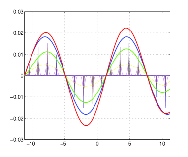
Figure 4.1 illustrates shapes of the assembled canonical vectors modulated by a $\sin$-harmonics imitating the construction of the Wannier-type functions.

Now we are able to estimate QTT ranks of the assembled canonical vectors representing the lattice sum. In this study, we analyze the canonical decomposition based on the initial (non-optimized) quadrature (2.7), where each term is obtained by sampling of a Gaussian on the uniform 3D grid. In practice, we apply the optimized quadrature obtained from the previous one by certain algebraic rank reduction [1]. This optimization procedure slightly modifies the shape of canonical vectors, however, the numerical tests indicate merely the same QTT ranks as predicted by our theory for the Gaussian-type vectors.

Lemma 4.4

For given tolerance $\varepsilon>0$, suppose that the set of Gaussian functions $S:=\{g_{k}=e^{-t_{k}^{2}\|x\|^{2}}\}$, $k=0,1,...,M$, representing canonical vectors in tensor decomposition $\mathbf{P}_{R}$, is specified by parameters in (2.4). Let us split the set $S$ into two subsets $S=S_{loc}\cup S_{glob}$, such that

$$S_{loc}:=\{g_{k}:a_{\varepsilon}(g_{k})\leq b\}\quad\mbox{and}\quad S_{glob}=S\setminus S_{loc}.$$

where $a_{\varepsilon}(g_{k})$ is defined by (4.1). Then the QTT-rank of each canonical vector $v_{q}$, $q=1,...,R$, in (3.3), where $R=M+1$, corresponding to $S_{loc}$ obeys the uniform in $L$ rank bound

$$r_{QTT}\leq C\log(1/\varepsilon).$$

For vectors in $S_{glob}$ we have the rank estimate

$$r_{QTT}\leq C\log(L/\varepsilon).$$

Proof. In our notation we have $1/(\sqrt{2}p_{k})=t_{k}=(k\log M)/M$, $k=1,...,M$ ($k=0$ is the trivial case). We omit the constant factor $\sqrt{2}$ to obtain $p_{k}=M/(k\log M)$.

For functions $g_{k}\in S_{loc}$, the relation (4.1) implies

$$O(1)=b\geq a_{\varepsilon}(g_{k})=\sqrt{2}p_{k}\log^{1/2}(1/\varepsilon),$$

implying the uniform bound $p_{k}\leq C$, and then the rank estimate $r_{QTT}\leq C\log(1/\varepsilon)$ in view of Proposition 4.1. Now we apply Lemma 4.2 to obtain the uniform in $L$ rank bound.

For globally supported functions in $S_{glob}$ we have $bL\geq a_{\varepsilon}\simeq p_{k}\log^{1/2}(1/\varepsilon)\geq b$, hence we will consider all these function on the maximal support of the size of supercell, $bL$, and set $a=bL$. Using the trigonometric representation as in the proof of Lemma 2 in [16], we conclude that for each fixed $k$ the shifted Gaussians, $g_{k,\ell}(x)=e^{-t_{k}^{2}\|x-\ell b\|^{2}}$ ($\ell=1,...,L$), can be approximated by shifted trigonometric series

$$G_{r}(x-b\ell)=\sum\limits_{m=0}^{M}C_{m}p\mathrm{e}^{-\frac{\pi^{2}m^{2}p^{2}}{2a^{2}}}\cos\left(\dfrac{\pi m(x-b\ell)}{a}\right),\quad a=bL,$$

which all have the common trigonometric basis containing about $rank_{QTT}(G_{r})=O(\log(\frac{p_{k}}{\varepsilon}))=O(\log(\frac{bL}{\varepsilon}))$ terms. Hence the sum of shifted Gaussian vectors over $L$ unit cells will be approximated with the same QTT-rank bound as each individual term in this sum, which proves the assertion.   

Figure 4.2: QTT-ranks of the canonical vectors of a single 3D Newton kernel discretized on a cubic grids of size $n^{3}=16384^{3},\,32768^{3},\,65536^{3}$ and $131072^{3}$.

Based on the previous statements, we arrive at the following result.

Theorem 4.5

The projected tensor of $v_{c_{L}}$ for the full sum over a single charge can be presented by the rank-$R$ QTT-canonical tensor

$${\bf P}_{c_{L}}=\sum\limits_{q=1}^{R}({\cal Q}\sum\limits_{k_{1}=1}^{L}{\cal W}_{\nu({k_{1}})}{\bf p}^{(1)}_{q})\otimes({\cal Q}\sum\limits_{k_{2}=1}^{L}{\cal W}_{\nu({k_{2}})}{\bf p}^{(2)}_{q})\otimes({\cal Q}\sum\limits_{k_{3}=1}^{L}{\cal W}_{\nu({k_{3}})}{\bf p}^{(3)}_{q}),$$ (4.3)

where the QTT-rank of each canonical vector is bounded by $r_{QTT}\leq C\log(L/\varepsilon)$. The computational cost is estimated by $O(RLr_{QTT}^{3})$, while the storage size scales as $O(R\log^{2}(L/\varepsilon))$.

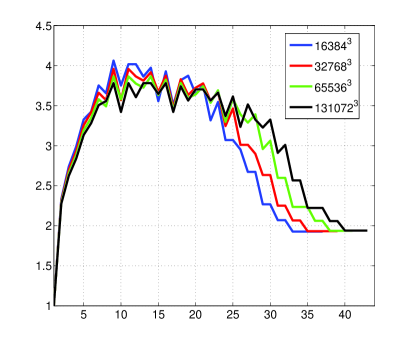
Figure 4.2 represents QTT-ranks of the canonical vectors of a single 3D Newton kernel discretized on a large cubic grids.

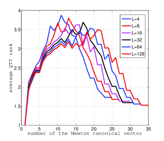
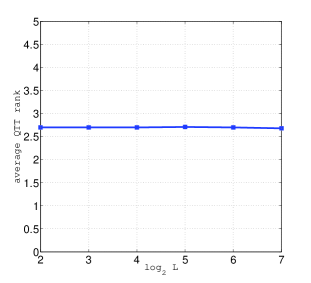
Figure 4.3 demonstrates that the average QTT ranks of the assembled canonical vectors for $k=1,...,R$, scale logarithmically both in $L$ and in the total grid-size $n=N_{L}$.

Figure 4.3: Left: QTT ranks of the assembled canonical vectors vs. $L$ for fixed grid size $N^{3}=16384^{3}$. Right: Average QTT-ranks over $R$ canonical vectors vs. $\log L$ for 3D evaluation of the $L\times 1\times 1$ chain of Hydrogen atoms on $N\times N\times N$ grids, $N=2048,\,4096,\,8192$, $16384$.

5 Conclusions

We introduce the method of assembled rank-structured calculation of large $L\times L\times L$ lattice sums of potentials discretized on $N\times N\times N$ 3D Cartesian grid in a box and for the supercell in periodic boundary conditions.

Advantages of the tensor approach applied to the lattice summation problem are achieved due to combination of two basic concepts. First, we apply the low-rank separable tensor-product representation of a single Newton kernel discretized on a fine $N\times N\times N$ spacial grid, that can be used as the master tensor for the translation along any lattice vector. Second, the global 3D product-type geometry in the location of interaction potentials enables us to employ the assembled summation of shifted low-rank canonical tensors. The latter allows to adapt tensor calculus to reduce the 3D summation to 1D sums of $N$-vectors.

The total lattice sum of shifted potentials in a box is proven to preserve the same canonical rank as that for a single Newton kernel.

For the case of lattice sums in a box our approach exhibits linear scaling in $L$, for both computational work and storage size, reducing dramatically the numerical costs compared with other summation methods. For example, computation of a sum of $10^{6}$ electrostatic potentials of Hydrogen nuclei in a box takes about $2$ seconds, when using our algorithms implementation in Matlab on a terminal of 8 AMD Opteron cluster (see Table 3.1). Comparison of the direct canonical sums of the electrostatic potentials and the assembled lattice tensor summation demonstrates the accuracy at the level of machine precision, $10^{-14}$.

In the periodic setting, the storage size is uniformly bounded in $L$.

For both models, we prove that QTT approximation method reduces the complexity to logarithmic scaling in the total grid size, $O(\log N)$. This suggests the efficient approach to numerical simulations on large $L\times L\times L$ lattices since the limitations on the spacial grid-size are essentially relaxed.

It is worth to note that the sum of electrostatic potentials is calculated in a whole computational box/supercell in a convenient structured form, which is suitable for further numerical treatment of the 3D quantities involved by using tensor methods in 1D complexity, for example, integration, differentiation, multiplication with a function, etc.

This approach can be also applied to a wide class of commonly used chemical potentials, in particular, to Coulomb-type, Yukawa, Helmholtz, Slater, Stokeslet, Lennard-Jones or van der Waals interactions. In all these cases the low-rank tensor decomposition can be proved to exist and can be constructed by the analytic-algebraic methods as in the case of Newton kernel.

6 Appendix: Basics of rank-structured tensor formats and operations

Separable representation of the multidimensional arrays in the Tucker and canonical tensor formats, were since long known in the computer science community [32], where they were mostly used in processing of the multidimensional experimental data in chemometrics, psychometrics and in signal processing. The remarkable approximating properties of the Tucker and canonical decomposition for wide classes of function related tensors were revealed in [27, 30], promoting its usage as a tool for the numerical treatment of the multidimensional problems in numerical analysis. An introductory description of tensor formats for function related tensors and tensor-structured numerical methods for calculation of multidimensional functions and operators is presented in [9, 46].

A tensor is a multidimensional array given by a $d$-tuple index set,

$${\bf A}=[a_{i_{1},...,i_{d}}]\in\mathbb{R}^{n_{1}\times\ldots\times n_{d}},\quad i_{\ell}\in\{1,\ldots,n_{\ell}\}.$$

It is an element of a linear vector space equipped with the Euclidean scalar product. For tensor with equal sizes $n_{\ell}=n$, $\ell=1,\ldots d$, the required storage is $n^{\otimes d}$. To get rid of the exponential growth of the tensor with the dimension $d$, one can employ the rank-structured representations of the multidimensional arrays.

As a building block for such representation we use a rank-$1$ tensor, which is a tensor product of vectors in each dimension,

$${\bf A}={\bf a}^{(1)}\otimes...\otimes{\bf a}^{(d)}\in\mathbb{R}^{n_{1}\times\ldots\times n_{d}}$$

with entries $a_{i_{1},\ldots i_{d}}=a^{(1)}_{i_{1}}\cdot\cdot\cdot a^{(d)}_{i_{d}}$.

Taking a sum of $R$ rank-$1$ tensors with some weights $c_{k}$ one comes to the canonical rank-$R$ representation,

$${\bf A}=\sum\limits_{i=1}^{R}c_{i}{\bf a}_{i}^{(1)}\otimes\ldots\otimes{\bf a}_{i}^{(d)},\quad c_{i}\in\mathbb{R},$$ (6.1)

where ${\bf a}_{i}^{(\ell)}$ are normalized vectors. The tensor in the canonical format requires storage $O(dnR)$. Sometimes ${\bf a}_{i}^{(\ell)}$, $\ell=1,2,\;\ldots,d$, are called the ”skeleton“ vectors of the canonical rank-$R$ tensor representation, while the matrices $A^{(\ell)}=[{\bf a}_{1}^{(\ell)},\ldots,{\bf a}_{R}^{(\ell)}]$ obtained by sticking together all vectors of the same mode ${\bf a}_{i}^{(\ell)}$, ($i=1,2,\ldots,R$) are called ”factor matrices” of the canonical tensor.

The Tucker decomposition is constructed using the orthogonal projection of the original tensor by the orthogonal matrices. It is also a sum of the tensor products,

$${\bf A}={\sum}_{\nu_{1}=1}^{r_{1}}\ldots{\sum}^{r_{d}}_{{\nu_{d}}=1}\beta_{\nu_{1},\ldots,\nu_{d}}\,{\bf a}^{(1)}_{\nu_{1}}\otimes\ldots\otimes{\bf a}^{(d)}_{\nu_{d}},\quad\ell=1,\ldots,d,$$

where ${\bf r}=(r_{1},...,r_{d})$ is the Tucker rank, $\boldsymbol{\beta}=[\beta_{\nu_{1},...,\nu_{d}}]$ is the core tensor, and the set of orthonormal vectors ${\bf a}^{(\ell)}_{\nu_{\ell}}\in\mathbb{R}^{n_{\ell}}$, form the orthogonal matrices of the Tucker projection.

The rank-structured tensor representation provides 1D complexity of multilinear operations with multidimensional tensors. Rank-structured tensor representation provides fast multi-linear algebra with linear complexity scaling in the dimension $d$.

For given canonical tensors ${\bf A}$ and ${\bf B}$ with the ranks $R_{a}$ and $R_{b}$, respectively, their Euclidean scalar product can be computed by

$$\left\langle{\bf A},{\bf B}\right\rangle:=\sum\limits_{i=1}^{R_{a}}\sum\limits_{j=1}^{R_{b}}c_{i}c_{j}\prod\limits_{\ell=1}^{d}\left\langle{\bf a}_{i}^{(\ell)},{\bf b}_{j}^{(\ell)}\right\rangle,$$ (6.2)

at the expense $O(dnR_{a}R_{b})$. The Hadamard product of tensors ${\bf A}$, ${\bf B}$ given in the form (6.1) is calculated in $O(dnR_{a}R_{b})$ operations by 1D point-wise products of vectors,

$${\bf A}\odot{\bf B}:=\sum\limits_{i=1}^{R_{a}}\sum\limits_{j=1}^{R_{b}}c_{i}c_{j}\left({\bf a}_{i}^{(1)}\odot{\bf b}_{j}^{(1)}\right)\otimes\ldots\otimes\left({\bf a}_{i}^{(d)}\odot{\bf b}_{j}^{(d)}\right).$$ (6.3)

Summation of two tensors in the canonical format ${\bf C}={\bf A}+{\bf B}$ is performed by a simple concatenation of their factor matrices, $A^{(\ell)}=[{\bf a}_{1}^{(\ell)},\ldots,{\bf a}_{R_{a}}^{(\ell)}]$ and $B^{(\ell)}=[{\bf b}_{1}^{(\ell)},\ldots,{\bf b}_{R_{b}}^{(\ell)}]$,

$$C^{(\ell)}=[{\bf a}_{1}^{(\ell)},\ldots,{\bf a}_{R_{a}}^{(\ell)},{\bf b}_{1}^{(\ell)},\ldots,{\bf b}_{R_{b}}^{(\ell)}].$$ (6.4)

The rank of the resulting canonical tensor is $R_{c}=R_{a}+R_{b}$.

In electronic structure calculations, the 3D convolution transform with the Newton kernel, $\frac{1}{\|x-y\|}$, is the most computationally expensive operation. The tensor method to compute convolution over large $n\times n\times n$ Cartesian grids in $O(n\log n)$ complexity was introduced in [28].
Given canonical tensors ${\bf A}$, ${\bf B}$ in a form (6.1), their convolution product is represented by the sum of tensor products of $1D$ convolutions,

$${\bf A}\ast{\bf B}=\sum\limits_{i=1}^{R_{a}}\sum\limits_{j=1}^{R_{b}}c_{i}c_{j}\left({\bf a}_{i}^{(1)}\ast{\bf b}_{j}^{(1)}\right)\otimes\left({\bf a}_{i}^{(2)}\ast{\bf b}_{j}^{(2)}\right)\otimes\left({\bf a}_{i}^{(3)}\ast{\bf b}_{j}^{(3)}\right),$$ (6.5)

where ${\bf a}_{k}^{(\ell)}\ast{\bf b}_{m}^{(\ell)}$ is the convolution product of $n$-vectors. The cost of tensor convolution in both storage and time is estimated by $O(R_{a}R_{b}n\log n)$. It considerably outperforms the conventional 3D FFT-based algorithm of complexity $O(n^{3}\log n)$ [31].

In tensor-structured numerical methods the calculation of the $3D$ convolution integrals is replaced by a sequence of $1D$ scalar and Hadamard products, and $1D$ convolution transforms [31, 9]. However, the sequences of rank-structured operations lead to increasing of tensor ranks since they are multiplied. For rank reduction, for example, the canonical-to-Tucker and Tucker-to-canonical algorithms can be used [30, 31, 9].

The matrix-product states (MPS) decomposition is since long used in quantum chemistry and quantum information theory [44, 43]. The particular case of MPS representation is called a tensor train (TT) format [38]. Any entry of a $d$th order tensor in this format is given by

$$a(i_{1},i_{2},\ldots,i_{d})=A^{(1)}_{i_{1}}A^{(2)}_{i_{2}}\ldots A^{(d)}_{i_{d}},$$ (6.6)

where each $A^{(k)}_{i_{k}}=A^{(k)}(\alpha_{k-1},i_{k},\alpha_{k})$ is $r_{k-1}\times r_{k}$ matrix depending on $i_{k}$ with the convention $r_{0}=r_{d}=1$. Storage size for $n^{\otimes d}$ TT tensor is bounded by $O(dr^{2}n)$, $r=\max{r_{k}}$. The algebraic operations on TT tensors can be implemented with linear complexity scaling in $n$ and $d$.

In 2009 the quantics-TT (QTT) tensor approximation method was introduced and rigorously proved to provide logarithmic scaling in storage for a wide class of function generated vectors and multidimensional tensors, see also [29]. In particular, the QTT representation of function-related vectors of size $N=q^{L}$, ($q=2,3,...$) needs only

$$q\cdot L\cdot r^{2}\ll q^{L}$$

numbers to store, where $r$ is the QTT-rank of $q\times q\times...\times q$ tensor of order $L$, reshaped from the initial vector by $q$-adic folding [29]. For example, the $N$-vector ${\bf x}=[x_{i}]$ of size $N=q^{L}$ is reshaped to its quantics image in $\mathbb{Q}_{L}:=\bigotimes_{\ell=1}^{L}\mathbb{R}^{q}$ via $q$-coding,

$$i-1=\sum_{\ell=1}^{L}(j_{\ell}-1)q^{\ell-1},\quad j_{\ell}\in\{1,2,...,q\}.$$

Though the optimal choice is shown to be $q=2$ or $q=3$, the numerical implementations are usually performed with $q=2$ (binary coding).

In [29] it was proven that the rank parameter $r$ in the QTT approximation is a small constant for a wide class of functions discretized on the uniform grid. For example, $r=1$ for complex exponents, $r=2$ for trigonometric functions and for Chebyshev polynomials (sampled on Chebyshev-Gauss-Lobatto grid), and $r\leq m+1$ for polynomials of degree $m$ (see also [21]). These properties are extended to various combinations of above functions.

The QTT approximation method enables the multidimensional vector transforms with logarithmic complexity scaling, $O(\log N)$. For example, we mention the superfast FFT [15], Laplacian inverse [26] and wavelet [47] transforms.

References

- [1] C. Bertoglio, and B.N. Khoromskij. Low-rank quadrature-based tensor approximation of the Galerkin projected Newton/Yukawa kernels. Comp. Phys. Communications, 183(4) (2012) 904–912.
- [2] Bloch, André, ”Les theoremes de M. Valiron sur les fonctions entieres et la theorie de l’uniformisation”. Annales de la faculte des sciences de l’universite de Toulose 17 (3): 1-22 (1925). ISSN 0240-2963.
- [3] Boys, S. F., Cook, G. B., Reeves, C. M. and Shavitt, I. (1956). Automatic Fundamental Calculations of Molecular Structure. Nature, 178: 1207-1209.
- [4] D. Braess. Nonlinear approximation theory. Springer-Verlag, Berlin, 1986.
- [5] Pollock, E. L. and Glosli, J. Comments on p(3)m, fmm and the Ewald method for large periodic Coulombic systems. Comput. Phys. Comm. 95, 93-110 (1996).
- [6] D. Braess. Asymptotics for the Approximation of Wave Functions by Exponential-Sums. J. Approx. Theory, 83: 93-103, (1995).
- [7] E. Cancés, V. Ehrlacher, and Y. Maday. Periodic Schrödinger operator with local defects and spectral pollution. SIAM J. Numer. Anal. v. 50, No. 6, pp. 3016-3035.
- [8] E. Cancés and C. Le Bris. Mathematical modeling of point defects in materials science. Math. Methods Models Appl. Sci. 23 (2013) 1795-1859.
-
[9]
Venera Khoromskaia.
Numerical Solution of the Hartree-Fock Equation by Multilevel Tensor-structured methods.
PhD thesis, TU Berlin, 2010.
http://opus4.kobv.de/opus4-tuberlin/frontdoor/index/index/docId/2780 - [10] V. Khoromskaia, D. Andrae, and B.N. Khoromskij. Fast and accurate 3D tensor calculation of the Fock operator in a general basis. Comp. Phys. Communications, 183 (2012) 2392-2404.
- [11] V. Khoromskaia. Black-box Hartree-Fock solver by tensor numerical methods. Comp. Meth. in Applied Math., Vol. 14 (2014) No.1, pp. 89-111.
- [12] B.N. Khoromskij, V. Khoromskaia, and H.-J. Flad. Numerical Solution of the Hartree-Fock Equation in Multilevel Tensor-structured Format. SIAM J. Sci. Comp. 33(1) (2011) 45-65.
- [13] T. Darten, D. York and L. Pedersen. Particle mesh Ewald: An method for Ewald sums in large systems. J. Chem. Phys., 98, 10089-10091, 1993.
- [14] M. Deserno and C. Holm. How to mesh up Ewald sums. I. A theoretical and numerical comparison of various particle mesh routines. J. Chem. Phys., 109(18): 7678-7693, 1998.
- [15] S.V. Dolgov, B.N. Khoromskij, and D. Savostyanov. Superfast Fourier transform using QTT approximation. J. Fourier Anal. Appl., 2012, vol.18, 5, 915-953.
- [16] S.V. Dolgov, B.N. Khoromskij, and I. Oseledets. Fast solution of multi-dimensional parabolic problems in the TT/QTT formats with initial application to the Fokker-Planck equation. SIAM J. Sci. Comput., 34(6), 2012, A3016-A3038.
- [17] R. Dovesi, R. Orlando, C. Roetti, C. Pisani, and V.R. Sauders. The Periodic Hartree-Fock Method and its Implementation in the CRYSTAL Code. Phys. Stat. Sol. (b) 217, 63 (2000).
- [18] Ewald P.P. Die Berechnung optische und elektrostatischer Gitterpotentiale. Ann. Phys 64, 253 (1921).
- [19] I.P. Gavrilyuk, W. Hackbusch and B.N. Khoromskij. Hierarchical Tensor-Product Approximation to the Inverse and Related Operators in High-Dimensional Elliptic Problems. Computing 74 (2005), 131-157.
- [20] L. Grasedyck, D. Kressner and C. Tobler. A literature survey of low-rank tensor approximation techniques. arXiv:1302.7121v1, 2013.
- [21] L. Grasedyck. Polynomial approximation in hierarchical Tucker format by vector-tensorization. Preprint 308, Institut fuer Geometrie und Praktische Mathematik, RWTH Aachen, 2010.
- [22] L. Greengard and V. Rochlin. A fast algorithm for particle simulations. J. Comp. Phys. 73 (1987) 325.
- [23] W. Hackbusch and B.N. Khoromskij. Low-rank Kronecker product approximation to multi-dimensional nonlocal operators. Part I. Separable approximation of multi-variate functions. Computing 76 (2006), 177-202.
- [24] T. Helgaker, P. Jørgensen, and J. Olsen. Molecular Electronic-Structure Theory. Wiley, New York, 1999.
- [25] Philippe H. Hünenberger. Lattice-sum methods for computing electrostatic interactions in molecular simulations. CP492, L.R. Pratt and G. Hummer, eds., 1999, American Institute of Physics, 1-56396-906-8/99.
- [26] V. Kazeev, and B.N. Khoromskij. Explicit low-rank QTT representation of Laplace operator and its inverse. SIAM Journal on Matrix Anal. and Appl., 33(3), 2012, 742-758.
- [27] B.N. Khoromskij, Structured Rank- Decomposition of Function-related Tensors in . Comp. Meth. in Applied Math., 6 (2006), 2, 194-220.
- [28] B.N. Khoromskij. Fast and Accurate Tensor Approximation of a Multivariate Convolution with Linear Scaling in Dimension. J. Comp. Appl. Math. 234 (2010) 3122-3139.
- [29] B.N. Khoromskij. -Quantics Approximation of - Tensors in High-Dimensional Numerical Modeling. Constructive Approx. 34 (2011) 257–280. (Preprint 55/2009 MPI MiS, Leipzig 2009.)
- [30] B. N. Khoromskij and V. Khoromskaia. Low Rank Tucker Tensor Approximation to the Classical Potentials. Central European J. of Math., 5(3) 2007, 1-28.
- [31] B.N. Khoromskij and V. Khoromskaia. Multigrid tensor approximation of function related multi-dimensional arrays. SIAM J. Sci. Comp. 31(4) (2009) 3002-3026.
- [32] T.G. Kolda and B.W. Bader. Tensor Decompositions and Applications. SIAM Rev. 51(3) (2009) 455–500.
- [33] K.N. Kudin, and G.E. Scuseria, Revisiting infinite lattice sums with the periodic Fast Multipole Method, J. Chem. Phys. 121, 2886-2890 (2004).
- [34] O.V. Yazyev, E.N. Brothers, K.N. Kudin, and G.E. Scuseria, A finite temperature linear tetrahedron method for electronic structure calculations of periodic systems, J. Chem. Phys. 121, 2466-2470 (2004).
- [35] S. A. Losilla, D. Sundholm, J. Juselius. The direct approach to gravitation and electrostatics method for periodic systems. J. Chem. Phys. 132 (2) (2010) 024102.
- [36] D. Lindbo and A.-K. Tornberg. Fast and spectrally accurate Ewald summation for 2-periodic electrostatic systems. J. Chem. Phys. 136:164111, 2012, doi: 10.1063/1.4704177.
- [37] M. Lorenz, D. Usvyat, and M. Schütz. Local ab initio methods for calculating optical band gaps in periodic systems. I. Periodic density fitted local configuration interaction singles method for polymers. J. Chem. Phys. 134, 094101 (2011); doi: 10.1063/1.3554209.
- [38] I.V. Oseledets. Tensor-train decomposition. SIAM J. Sci. Comp., 33(5), 2011, pp. 2295-2317.
- [39] C. Pisani, M. Schütz, S. Casassa, D. Usvyat, L. Maschio, M. Lorenz, and A. Erba. CRYSCOR: a program for the post-Hartree-Fock treatment of periodic systems. Phys. Chem. Chem. Phys., 2012, 14, 7615-7628.
- [40] E.L. Pollock, and Jim Glosli. Comments on , , and the Ewald method for large periodic Coulombic systems. Computer Phys. Communication 95 (1996), 93-110.
- [41] A.Y. Toukmaji, and J. Board Jr. Ewald summation techniques in perspective: a survey. Computer Phys. Communication 95 (1996), 73-92.
- [42] Elena Voloshina, Denis Usvyat, Martin Schütz, Yuriy Dedkov and Beate Paulus. On the physisorption of water on graphene: a CCSD(T) study. Phys. Chem. Chem. Phys., 2011, 13, 12041-12047.
- [43] F. Verstraete, D. Porras, and J.I. Cirac, DMRG and periodic boundary conditions: A quantum information perspective. Phys. Rev. Lett., 93(22): 227205, Nov. 2004.
- [44] S.R. White. Density-matrix algorithms for quantum renormalization groups. Phys. Rev. B, v. 48(14), 1993, 10345-10356.
- [45] B.N. Khoromskij. Introduction to Tensor Numerical Methods in Scientific Computing. Lecture Notes, Preprint 06-2011, University of Zuerich, Institute of Mathematics, 2011, pp 1 - 238. http://www.math.uzh.ch/fileadmin/math/preprints/0611.pdf
- [46] B.N. Khoromskij. Tensors-structured Numerical Methods in Scientific Computing: Survey on Recent Advances. Chemometr. Intell. Lab. Syst. 110 (2012), 1-19.
- [47] Boris N. Khoromskij, and Sentao Miao. Superfast Wavelet Transform Using QTT Approximation. I: Haar Wavelets. Preprint 103/2013, MPI MiS, Leipzig 2013; (CMAM 2014, to appear).
- [48] V. Khoromskaia and B.N. Khoromskij. Grid-based lattice summation of electrostatic potentials by low-rank tensor approximation. Preprint 116/2013, MPI MiS, Leipzig 2013.