Phase diagram of two-dimensional hard ellipses
Abstract
We report the phase diagram of two-dimensional hard ellipses as obtained from replica exchange Monte Carlo simulations. The replica exchange is implemented by expanding the isobaric ensemble in pressure. The phase diagram shows four regions: isotropic, nematic, plastic, and solid (letting aside the hexatic phase at the isotropic-plastic two-step transition [PRL 107, 155704 (2011)]). At low anisotropies, the isotropic fluid turns into a plastic phase which in turn yields a solid for increasing pressure (area fraction). Intermediate anisotropies lead to a single first order transition (isotropic-solid). Finally, large anisotropies yield an isotropic-nematic transition at low pressures and a high-pressure nematic-solid transition. We obtain continuous isotropic-nematic transitions. For the transitions involving quasi-long-range positional ordering, i. e. isotropic-plastic, isotropic-solid, and nematic-solid, we observe bimodal probability density functions. This supports first order transition scenarios.
pacs:
64.30.-t, 64.70.mf, 61.30.CzI Introduction
Two-dimensional models are frequently employed as idealizations of quasi-2D experimental setups, such as strongly confined colloids or colloidal thin films Loewen (2009); Tkalec and Muševič (2013); Arciniegas et al. (2014). In turn, quasi-2D mesophases and nanocrystals can be used as basic units for the synthesis of superlattice structures Quan and Fang (2010), multilayer arrangements by means of layer-by-layer assembly Schmitt et al. (1993); Decher (1997), and for template assisted assembly processes Rycenga, Camargo, and Xia (2009). These applications have encouraged several experimental and simulation studies on the behavior of 2D-confined nanocrystals of different shapes Qi et al. (2012). For instance, experiments and simulations have shown that needles, squares, octapods, and ellipsoidal anisotropic particles produce a rich mesophase behavior when confined to a quasi-2D plane Frenkel and Eppenga (1985); Cuesta and Frenkel (1990); Donev et al. (2006); Avendano and Escobedo (2012); Shah et al. (2012); Qi et al. (2012, 2013). For designing such arrangements, it is important to take into account the directional nature of entropic forces acting on anisotropic particles Damasceno, Engel, and Glotzer (2012); van Anders et al. (2014), i. e. the effective forces that result from a system’s statistical tendency to increase its entropy. In particular, for hard systems, these are the only forces acting on the particles and are responsible for the different type of phase transitions appearing at different densities and particle-anisotropies. Directionality makes anisotropic particles show, in general, a much richer phase behavior than isotropic ones.
Probably the most simple 2D-system is the hard disk model. Nonetheless, the phase transition this model shows is, to say the least, hard to elucidate. In the first place, the solid phase for 2D-systems has quasi-long-range but not true-long-range positional order. That is, positional correlations decay to zero following a power-law. On the other hand, bond orientational correlations are indeed, long-ranged. Hence, a 2D-solid is not a crystal, since true crystals preserve both, bond orientational order and positional order for all distances. In the second place, in-between the solid and the liquid, Kosterlitz, Thouless, Halperin, Nelson, and Young (KTHNY) Kosterlitz and Thouless (1973); Halperin and Nelson (1978) proposed the existence of a hexatic phase. This phase is characterized by quasi-long-range bond orientational correlations, similar to a two-dimensional nematic where orientation is also quasi-long-range ordered Straley (1971); Frenkel and Eppenga (1985); Bates and Frenkel (2000); Zheng and Han (2010); Xu et al. (2013), but with a sixfold rather than twofold anisotropy. In their scenario, the solid melts into a hexatic phase, following a dislocation unbinding process, before turning into a liquid by means of disclination unbinding, for decreasing pressure. The theory predicts the two transitions to be continuous. The KTHNY two-step continuous transition and a single first order transition have been the two of several scenarios which have larger support Jaster (1999). Quite recent long-scale computer simulations (containing particles) strongly suggest a liquid-hexatic first order transition, followed by a continuous hexatic-solid transition Bernard and Krauth (2011).
A possible way to include anisotropy in the 2D-system is to replace disks by ellipses. This looks natural since circles (disks) are a particular type of ellipses (with both focal points at the same location), or the other way around, ellipses are the generalization of circles. Thus, ellipses on a plane can be seen as the most simple anisotropic model in 2D. Studies on ellipses are mostly focused on the isotropic-nematic transition Xu et al. (2013). Monte Carlo simulations of Vieillard-Baron are the first of this kind Vieillard-Baron (1972) (there is a previous determination of the structure factor of a hard ellipse nematic phase Levesque, Schiff, and Vieillard-Baron (1969)). For an aspect radio three different phases are identified: isotropic, nematic, and solid. For a quasi-spherical case, a phase “analogous to the plastic crystal phase” was found Vieillard-Baron (1972). Here, plastic crystal means the existence of positional order and the lack of orientational order. More evidence on the isotropic-nematic transition of hard anisotropic particles, needles Frenkel and Eppenga (1985) and rods Bates and Frenkel (2000), revealed that this type of transition is continuous. In addition, Cuesta and Frenkel Cuesta and Frenkel (1990) showed that there is no stable nematic phase in hard ellipses for . A recent work on hard ellipses by Xu et. al. Xu et al. (2013) gives much further details on the isotropic-plastic and isotropic-nematic transition of hard ellipses. In this last work, as well as in reference Foulaadvand and Yarifard (2013), transport properties of fluid phases are also studied. However, details on the large area fraction region of the phase diagram, which includes both, the isotropic-solid and plastic-solid transitions, remain elusive.
The main goal of this paper is to report the whole phase diagram of hard ellipses in the anisotropy region . For this purpose, we are implementing replica exchange Monte Carlo simulations (REMC) by performing a pressure extension of the isobaric ensemble. This way, area fluctuations are accessed on each set pressure providing useful information at the transitions. We detect four phases (letting aside the hexatic phase in-between the isotropic and plastic phases Bernard and Krauth (2011)) which are isotropic, plastic, solid, and nematic. At low anisotropies , we have obtained a low-pressure isotropic-plastic first order transition (a probable two-step transition involving a hexatic phase, with a first order isotropic-hexatic transition followed by a subtle and continuous hexatic-plastic transition, taking into account Bernard and Krauth conclusions Bernard and Krauth (2011)) and a high-pressure plastic-solid transition. Intermediate anisotropies, yield a single isotropic-solid transition (confirming Cuesta and Frenkel results Cuesta and Frenkel (1990) for ). Finally, for , a low-pressure isotropic-nematic continuous transition and a high-pressure nematic-solid transition are found.
II Simulation details
To detect overlaps we are following the 3D analytical approach of Rickayzen Rickayzen (1998) while restricting the particles geometrical centers to move in a 2D-plane and their axis of revolution to rotate inside it. The Rickayzen-Berne-Pechukas (RBP) expression is given by Rickayzen (1998)
| (1) |
where
| (2) |
| (3) |
In this expression, and are the major and minor axes of the ellipses, respectively. We take as the length unit and vary to obtain different anisotropies. The aspect ratio is given by , such that . corresponds to the disks case. and are unit vectors along the smallest diameters of ellipsoids and , respectively. is the unit vector along the line joining the geometric particle centers. In addition, is introduced to further approach the exact Perram and Wertheim numerical solution Perram et al. (1984); Perram and Wertheim (1985). values are given in reference de J. Guevara-Rodríguez and Odriozola (2011). The average difference between the analytical approach and the exact numerical solution is always small de J. Guevara-Rodríguez and Odriozola (2011).
To avoid the inherent hysteresis associated to transitions as far as possible Bautista-Carbajal, Moncho-Jordá, and Odriozola (2013), we are implementing the replica exchange Monte Carlo technique Marinari and Parisi (1992); Lyubartsev et al. (1992); Hukushima and Nemoto (1996). It is based on the definition of an extended ensemble whose partition function is given by , being the partition function of ensemble and the number of ensembles. replicas are employed to sample this extended ensemble, each one placed at each ensemble. The definition of allows the introduction of swap trial moves between any two replicas, whenever the detail balance condition is satisfied. Since hard particles are being studied, it is convenient to expand isobaric-isothermal ensembles in pressure Odriozola (2009). This way, the partition function of the extended ensemble is given by Okabe et al. (2001); Odriozola (2009)
| (4) |
where is the partition function of the isobaric-isothermal ensemble of the system at pressure , temperature , and with particles.
The ensembles are sampled through a standard implementation, involving independent trial displacements, rotations of single ellipsoids, and volume changes. To increase the degrees of freedom of our relatively small systems (), we have implemented non-orthogonal parallelogram cells. Thus, sampling also includes trial changes of the angles and relative length sides of the cell lattice vectors. The probabilities for choosing any adjacent pairs of replicas are set equal and the following acceptance rule is employed Odriozola (2009)
| (5) |
where is the volume difference between replicas and and is the reciprocal temperature. Adjacent pressures must be close enough to provide reasonable swap acceptance rates.
Simulations are started from a packed triangular arrangement of disks which are elongated in a certain in-plane direction by a factor . Conversely to the stretching of spheres, this procedure leads to the largest packed arrangement of ellipses Donev et al. (2004). It is faster to get a stationary state by decompressing packed cells than by compressing lose random configurations Bautista-Carbajal, Moncho-Jordá, and Odriozola (2013). We first perform the necessary trial moves at the desired state points to ensure the development of a stationary state (on the order of trial moves). During this process we adjust maximum displacements to get acceptance rates close to 0.3. We also relocate set pressures, initially set by following a geometric progression with the replica index, to obtain similar swap acceptance rates for all pairs of adjacent ensembles Rathore, Chopra, and de Pablo (2005). Once this is done, we then perform additional sampling trials where maximum particle displacements, maximum rotational displacements, maximum volume changes, maximum changes of the lattice vectors, and pressures are fixed. Verlet neighbor lists Donev, Torquato, and Stillinger (2005) are used to improve performance. We set ellipsoids and or , depending on the pressure range to be covered. seems enough in view of Xu et. al. analysis of system size effects Xu et al. (2013). More details on the employed methods are given in previous works Bautista-Carbajal, Moncho-Jordá, and Odriozola (2013).
III Results
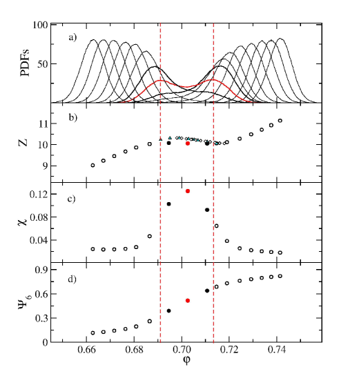
We start this section with the equation of state (EOS) for the case, that is, for a system of disks on a plane. The EOS is shown in panel b) of figure 1, i. e. where , , , , and is the area of the simulation cell. In this plot we are also including as solid triangles the results of the large scale MC simulations with carried out by Jaster Jaster (1999), and as diamonds those of Bernard and Krauth Bernard and Krauth (2011) with . These results are set in the liquid-solid transition region where size effects are expected to be present. As can be seen, differences with our data are not very large, though. Nonetheless, even very large systems show small differences with increasing the system size Bernard and Krauth (2011). In addition to the EOS, we are including the probability density functions (PDFs) from where the averages are taken (panel a), the dimensionless isothermal compressibility (panel c), and the global order parameter (panel d) with where is the number of bonding particles to and is the angle between the -bond and an arbitrary fixed reference axis. All these data strongly suggest a first order transition. Nevertheless, the -plateau, the peak, and the development of an overall bond order are well known facts which do not constitute enough evidence to establish the nature of the liquid-solid transition. Indeed, there is not a general consensus on the nature of the fluid-solid hard disks transition. Among the different scenarios, the KTHNY theory Kosterlitz and Thouless (1973); Halperin and Nelson (1978) predicts a two-step transition where the fluid turns into a hexatic phase before the solid when increasing pressure. According to the KTHNY theory both transitions, i. e. fluid-hexatic and hexatic-solid, are continuous. Recent large scale () computer simulations, however, support the existence of a first order fluid-hexatic transition followed by a hexatic-solid continuous one Bernard and Krauth (2011) (a bubble formation, which is a hallmark of a first-order transition, is observed). This work reports a coexistence interval of for the fluid-hexatic transition and a second transition at . Hence, the hexatic phase would only take place at the interval .
Back to our results, we did obtain a PDF bimodal at the coexistence region. The curve is highlighted in panel a) of figure 1. This bimodal also supports the existence of a first order transition. From their peaks we obtain the coexistence region (we follow the histogram reweighting technique for determining the coexistence boundaries Ferrenberg and Swendsen (1988, 1989)). The vertical dashed lines of figure 1 point out the coexistence interval. Taking into account Bernard and Krauth conclusions, this coexistence should be fluid-hexatic. The hexatic-solid would be relatively close to , but we are not capturing this subtle continuous transition (Bernard and Krauth capture it from the shift of positional order decay from exponential to power-law, on a length scale of ). It should also be noted that our coexistence region is wider and shifted to the left as compared to the fluid-hexatic coexistence given in reference Bernard and Krauth (2011). This not so large mismatch is a consequence of finite size effects.
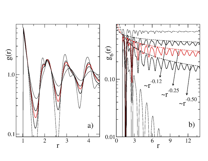
Letting aside the peaks of the PDF bimodal, the bond orientation radial correlation function is frequently employed to quantitatively identify the location of the transition from the isotropic liquid to the hexatic phase Xu et al. (2013). It is given by , where is the Kronecker delta function. The hexatic phase sets in when the function decays slower than with as pointed out elsewhere Kosterlitz and Thouless (1973); Halperin and Nelson (1978). We are showing the obtained curves in panel b) of figure 2 as obtained from the bimodal PDF shown in figure 1 and both adjacent set pressures. We are also including the curves for the highest and lowest set pressures as thin lines. As labeled in panel b), the thick dashed lines correspond to with , 0.25, and 0.50. We estimate these values to have relatively large error bars (though below 20) due to the small system size we are employing. Note that the decay matches the overall trend obtained from the bimodal. Hence, both criteria, the double-peak interval from the PDF bimodal and the trend coincide for the location of the liquid-hexatic boundary. We also observe that shows an inflection at this point (panel d) of figure 1). We are following the double-peak criteria for the phase diagram construction. In panel a) of the same figure we are including the corresponding radial distribution functions, . As expected, the structure builds up with increasing pressure, when the centers of mass of the particles arrange in a triangular lattice. Nonetheless, the positional correlations exponentially decay on a length scale of in the hexatic phase Bernard and Krauth (2011).
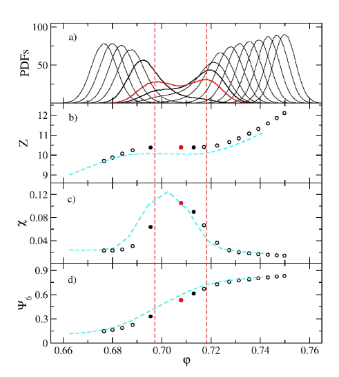
The equation of state for is shown in panel b) of figure 3 for the isotropic-plastic transition. As for the disks case, we are showing the probability density functions (PDFs) (panel a), the dimensionless isothermal compressibility (panel c), and the global order parameter (panel d). In panels b)-d) we include as cyan dashed lines the results obtained for to make the comparison easy. From all panels it becomes clear that the transition slightly shifted to higher densities and that the coexistence region narrows. In addition, the transition pressure also increases. All this is a consequence of the smaller entropy gain associated to the transition, since ellipses at the plastic phase do not pack as well as disks do Vieillard-Baron (1972). Furthermore, the shifting to higher densities and narrowing of the coexistence region continues for increasing . This trend remains up to , where the plastic region vanishes. We take this end to define the upper point of the low anisotropy region. This behavior is similar to those observed for spheroids, although the limit for the plastic region in this case is around 1.33 (for both sides, prolates and oblates) Bautista-Carbajal, Moncho-Jordá, and Odriozola (2013). Finally, we add here that for all studied our EOSs perfectly match those recently reported by Xu et. al. Xu et al. (2013) (not shown). Hence, their conclusions on the validity of several theoretical EOS Varga and Szalai (1998); Boublík (2011) remain unchanged when considering our results. However, as shown further in the text, we are pressurizing the system as much as necessary to access the solid phase.
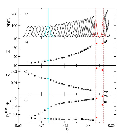
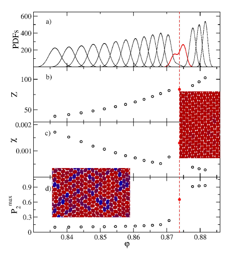
Figure 4 is an example of the EOS we have obtained for the large anisotropy region, . In particular, this figure is built for . Again, the PDFs, , , , and are shown in the panels. is the overall orientational order parameter (or nematic order parameter) which is given by the maximum eigenvalue of the tensor order parameter Cuesta and Frenkel (1990). In 2D , where is the angle between and an arbitrary fixed direction. On the other hand, the angle between the nematic director and the same arbitrary direction is . Alternatively, can be numerically obtained as described elsewhere Xu et al. (2013). Although decreases with the system size for the quasi-long-range nematic phase, its dependence is not strong Xu et al. (2013). Here two transitions are detected. A continuous one, at low compressions, which corresponds to an isotropic-nematic transition; and another that is discontinuous, at higher pressures, corresponding to a nematic-solid transition. No further transitions where observed at larger densities. The first transition is characterized by an increase of , an invariant , a tiny plateau of , and a small bump of . We are locating the isotropic-nematic transition at this bump. The PDF corresponding to this transition is clearly monomodal and supports a disclination unbinding scenario. We indeed obtain the same result for all anisotropies above . This result contradicts the Cuesta and Frenkel claim Cuesta and Frenkel (1990) that the isotropic-nematic transition is first order for . Hence, according to our data, there is no tricritical point on the isotropic-nematic transition line. At the second transition we find an increase of , a steep jump of , a large plateau of , and an important bump of . All these signatures appear together with the PDFs bimodals at the coexistence region. Note that for we are applying an stretching procedure with a factor to all bonds along the director direction previous to the computation. This is done in order to obtain for a perfect crystal and to take advantage of the definition.
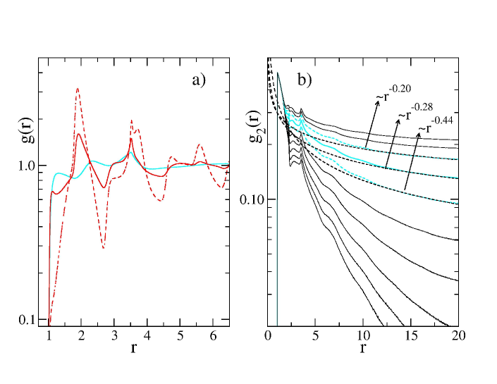
An alternative way for determining an upper bound to the exact value of the isotropic-nematic pressure is by means of analyzing the decay of the angular correlation function Straley (1971); Frenkel and Eppenga (1985); Bates and Frenkel (2000); Xu et al. (2013), . The 2D nematic phase is characterized by a power-law decay of with . This algebraic decay is a common feature for needles, rods, and ellipses confined to a plane. Thus, the subensemble average at the smallest pressure which leads to can be considered to produce the 2D-nematic phase the closest to the isotropic phase. The fittings of for the curves obtained in the vicinity of the isotropic-nematic pressure are shown in panel b) of figure 5. As labeled, we get for the transition determined according to the bump criterion. So, the fit analysis give rises to a slightly larger area fraction value for this transition than that obtained from the bump. This result is observed for all set anisotropies in the large anisotropy region. For completeness, panel a) of the same figure shows the radial distribution function obtained for the isotropic-nematic transition (cyan solid line) and those obtained before and after the nematic-solid transition (red dashed and solid lines).
Up to this point, we have focused on the isotropic-nematic and nematic-solid transitions for large anisotropies, and on the isotropic-plastic transition for low anisotropies occurring at relatively low pressures. Hence, the high-pressure plastic-solid transition is still missing. In order to capture this transition, we decompress perfect crystal cells with at high pressures. In particular, we are showing in figure 6 the results obtained for . In this plot we are including the PDFs, , , and . We are also including a couple of snapshots of part of the system cells showing the plastic (left) and solid (right) phases. As shown in panel b) of figure 6 a bimodal PDF curve builds up at (red and thick solid line). The histogram reweighting procedure Ferrenberg and Swendsen (1988, 1989) leads to a valley at (we are taking this point for the phase diagram). This curve corresponds to the solid symbols appearing at the other panels. Thus, for this PDF we observe a plateau, a bump, and a steep increase of . These features suggest a discontinuous transition and a small coexistence region. Nonetheless, the nature of the transition turns unclear for decreasing , as the bimodals seem to disappear, producing small kinks for (not shown).
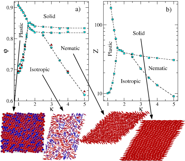
The phase diagram of hard ellipses is build by gathering the information for all studied . This is shown in the left panel of figure 7. At the right panel of the same figure we are including the compressibility factor, , at which the transitions take place. Furthermore, snapshots corresponding to the different phases are embedded in the figure. There we can see the plastic, isotropic, nematic, and solid phases. We are using a couple of square symbols to point out a coexistence region (in-between the couple) and single circles to point out a continuous transition. Note that we are marking the plastic-solid transition with circles, though a tiny coexistence is found for and 1.5. The dashed lines are guides to the eye. We are also including, as red triangles, the recently published data by Xu et. al. Xu et al. (2013). As can be seen, our results well agree with their predictions for both, the isotropic-plastic and the isotropic-nematic transitions. A comparison with data from Cuesta and Frenkel Cuesta and Frenkel (1990) and Vieillard-Baron Vieillard-Baron (1972) is provided in reference Xu et al. (2013).
The phase diagram of hard ellipses can be split into three regions. For low anisotropies, , there are two transitions. A low-pressure isotropic-plastic and a high-pressure plastic-solid transition. The first one, for and according to Bernard and Krauth findings Bernard and Krauth (2011), is an isotropic-hexatic first order transition followed by a subtle hexatic-solid transition. Consequently, for we obtain an isotropic-hexatic first order transition, which is the one we are capturing, followed by a mild hexatic-plastic continuous transition, which we are not detecting. The same conclusion is supported by the analysis given elsewhere Xu et al. (2013). Since the hexatic region is tiny, we are not including it in the phase diagram. The high pressure transition is also first order, at least for and 1.5. The second region corresponds to intermediate anisotropies, i. e. for . Here it is observed only a single isotropic-solid transition, where both, bond-orientational and orientational order develop. Finally, the third region corresponds to , where an isotropic-nematic transition occurs at low pressure and a nematic-solid transition appears at high pressure. This last transition is observed above an area fraction of for all . This quantitative result differs from those reported in references Vieillard-Baron (1972); Cuesta and Frenkel (1990) but agrees with Xu et. al. recent results Xu et al. (2013) (they found no sign of a transition involving a solid below ). We point out the weak dependence of the nematic-solid transition on . That is, it occurs at an almost constant area fraction and pressure (dependence on the pressure is larger, though). This suggests that the nematic-solid entropy gain associated to the transition practically holds with increasing , which in turn implies a similar gain on the system accessible area. In other words, the system behaves like being stretched in the nematic director direction while preserving occupied, accessible, and excluded areas.
IV Conclusions
We have reported the phase diagram of hard ellipses for anisotropies in the range . This is done by means of replica exchange Monte Carlo simulations. For we have found an isotropic phase at low pressures, a plastic one at intermediate pressures, and a solid one at high-pressures. In this case, the isotropic-plastic transition would probably be a two-step transition, with a small hexatic phase region in-between the isotropic and plastic regions. Our data support the existence of a first order transition in agreement with large-scale simulations of disks Bernard and Krauth (2011). In addition, the high pressure transition (plastic-solid) close to the upper bound of is also discontinuous. For weak anisotropies we have obtained a plastic-solid continuous transition. This would imply a tricritical point somewhere in the range . This picture, however, may probably change when considering larger system sizes in favor of the discontinuous scenario. For intermediate anisotropies, , the system shows only a single first order transition, isotropic-solid. Thus, nematic is absent here, in agreement with Cuesta and Frenkel early results Cuesta and Frenkel (1990). Finally, for , a continuous isotropic-nematic and a discontinuous nematic-solid transition are found. Our reported boundaries for the anisotropy regions are slightly different from those recently reported by Xu et. al. Xu et al. (2013). These differences mostly appear due to the fact that their study does not include results for area fractions above .
Finally, we think it is worth mentioning some similarities of hard anisotropic objects of variable aspect ratio between the 2D and 3D scenarios. One should note that the overall appearance obtained for the 2D phase diagram (Fig. 7) markedly resembles that of 3D systems of prolate and oblate ellipsoids, spherocylinders, and cut-spheres with variable aspect ratio (see references Bolhuis and Frenkel (1997); Wensink and Lekkerkerker (2009); Marechal et al. (2011); Bautista-Carbajal, Moncho-Jordá, and Odriozola (2013)). In particular, the isotropic-nematic transition line goes up in occupied area (volume) fraction upon decreasing the particle aspect ratio to eventually meet up with a strongly first-order and almost anisometric-independent fluid-solid transition. This point defines a critical aspect ratio below which the nematic phase ceases to be thermodynamically stable. This is a common feature for all referenced systems and most probably for other convex particle shapes in two and three dimensions.
Acknowledgements.
The authors thank Prof. Eliezer Braun for his fruitful discussions and support, Wen-Sheng Xu, Yan-Wei Li, Zhao-Yan Sun, and Li-Jia An for sharing their EOS data, Szabolcs Varga for useful suggestions, and the reviewers for their helpful comments. Indeed, the closing paragraph is taken from one of them. G.B-C thanks CONACyT for a Phd. scholarship. G.O thanks CONACyT Project No. 169125 for financial support.References
- Loewen (2009) H. Loewen, J. Phys.: Condens. Matter 21, 474203 (2009).
- Tkalec and Muševič (2013) U. Tkalec and I. Muševič, Soft Matter 9, 8140 (2013).
- Arciniegas et al. (2014) M. P. Arciniegas, M. R. Kim, J. De Graaf, R. Brescia, S. Marras, K. Miszta, M. Dijkstra, R. van Roij, and L. Manna, Nano Letters 14, 1056 (2014).
- Quan and Fang (2010) Z. Quan and J. Fang, Nano Today 5, 390 (2010).
- Schmitt et al. (1993) J. Schmitt, T. Grunewald, G. Decher, P. Pershan, K. Kjaer, and M. Losche, Macromolecules 26, 7058 (1993).
- Decher (1997) G. Decher, Science 277, 1232 (1997).
- Rycenga, Camargo, and Xia (2009) M. Rycenga, P. H. C. Camargo, and Y. Xia, Soft Matter 5, 1129 (2009).
- Qi et al. (2012) W. Qi, J. de Graaf, F. Qiao, S. Marras, L. Manna, and M. Dijkstra, Nano Letters 12, 5299 (2012).
- Frenkel and Eppenga (1985) D. Frenkel and R. Eppenga, Phys. Rev. A 31, 1776 (1985).
- Cuesta and Frenkel (1990) J. A. Cuesta and D. Frenkel, Phys. Rev. A 42, 2126 (1990).
- Donev et al. (2006) A. Donev, J. Burton, F. H. Stillinger, and S. Torquato, Phys. Rev. B. 73, 054109 (2006).
- Avendano and Escobedo (2012) C. Avendano and F. A. Escobedo, Soft Matter 8, 4675 (2012).
- Shah et al. (2012) A. A. Shah, H. Kang, K. L. Kohlstedt, K. H. Ahn, S. C. Glotzer, C. W. Monroe, and M. J. Solomon, Small 8, 1551 (2012).
- Qi et al. (2013) W. Qi, J. de Graaf, F. Qiao, S. Marras, L. Manna, and M. Dijkstra, J. Chem. Phys. 138, 154504 (2013).
- Damasceno, Engel, and Glotzer (2012) P. F. Damasceno, M. Engel, and S. C. Glotzer, ACS Nano 6, 609 (2012).
- van Anders et al. (2014) G. van Anders, N. K. Ahmed, R. Smith, M. Engel, and S. C. Glotzer, ACS Nano , DOI:10.1021/nn4057353 (2014).
- Kosterlitz and Thouless (1973) J. M. Kosterlitz and D. J. Thouless, J. Phys. C 6, 1181 (1973).
- Halperin and Nelson (1978) B. I. Halperin and D. R. Nelson, Phys. Rev. Lett. 41, 121 (1978).
- Straley (1971) J. P. Straley, Phys. Rev. A 4, 675 (1971).
- Bates and Frenkel (2000) M. A. Bates and D. Frenkel, J. Chem. Phys. 112, 10034 (2000).
- Zheng and Han (2010) Z. Zheng and Y. Han, J. Chem. Phys. 133, 124509 (2010).
- Xu et al. (2013) W. S. Xu, Y. W. Li, Z. Y. Sun, and L. J. An, J. Chem. Phys. 139, 024501 (2013).
- Jaster (1999) A. Jaster, Phys. Rev. E. 59, 2594 (1999).
- Bernard and Krauth (2011) E. P. Bernard and W. Krauth, Phys. Rev. Lett. 107, 155704 (2011).
- Vieillard-Baron (1972) J. Vieillard-Baron, J. Chem. Phys. 56, 4729 (1972).
- Levesque, Schiff, and Vieillard-Baron (1969) D. Levesque, D. Schiff, and J. Vieillard-Baron, J. Chem. Phys. 51, 3625 (1969).
- Foulaadvand and Yarifard (2013) M. E. Foulaadvand and M. Yarifard, Phys. Rev. E. 88, 052504 (2013).
- Rickayzen (1998) G. Rickayzen, Mol. Phys. 95, 393 (1998).
- Perram et al. (1984) J. W. Perram, M. S. Wertheim, J. L. Lebowitz, and G. O. Williams, Chem. Phys. Lett. 105, 277 (1984).
- Perram and Wertheim (1985) J. W. Perram and M. S. Wertheim, J. Comput. Phys. 58, 409 (1985).
- de J. Guevara-Rodríguez and Odriozola (2011) F. de J. Guevara-Rodríguez and G. Odriozola, J. Chem. Phys. 135, 084508 (2011).
- Bautista-Carbajal, Moncho-Jordá, and Odriozola (2013) G. Bautista-Carbajal, A. Moncho-Jordá, and G. Odriozola, J. Chem. Phys. 138, 064501 (2013).
- Marinari and Parisi (1992) E. Marinari and G. Parisi, Europhys. Lett. 19, 451 (1992).
- Lyubartsev et al. (1992) A. P. Lyubartsev, A. A. Martinovski, S. V. Shevkunov, and P. N. Vorontsov-Velyaminov, J. Chem. Phys. 96, 1776 (1992).
- Hukushima and Nemoto (1996) K. Hukushima and K. Nemoto, J. Phys. Soc. Jpn. 65, 1604 (1996).
- Odriozola (2009) G. Odriozola, J. Chem. Phys. 131, 144107 (2009).
- Okabe et al. (2001) T. Okabe, M. Kawata, Y. Okamoto, and M. Mikami, Chem. Phys. Lett. 335, 435 (2001).
- Donev et al. (2004) A. Donev, F. H. Stillinger, P. M. Chaikin, and S. Torquato, Phys. Rev. Lett. 92, 255506 (2004).
- Rathore, Chopra, and de Pablo (2005) N. Rathore, M. Chopra, and J. J. de Pablo, J. Chem. Phys. 122, 024111 (2005).
- Donev, Torquato, and Stillinger (2005) A. Donev, S. Torquato, and F. H. Stillinger, J. Comput. Phys. 202, 737 (2005).
- Ferrenberg and Swendsen (1988) A. M. Ferrenberg and R. H. Swendsen, Phys. Rev. Lett. 61, 2635 (1988).
- Ferrenberg and Swendsen (1989) A. M. Ferrenberg and R. H. Swendsen, Phys. Rev. Lett. 63, 1195 (1989).
- Varga and Szalai (1998) S. Varga and I. Szalai, Mol. Phys. 95, 515 (1998).
- Boublík (2011) T. Boublík, Mol. Phys. 109, 1575 (2011).
- Bolhuis and Frenkel (1997) P. Bolhuis and D. Frenkel, J. Chem. Phys. 106, 666 (1997).
- Wensink and Lekkerkerker (2009) H. H. Wensink and H. N. W. Lekkerkerker, Mol. Phys. 107, 2111 (2009).
- Marechal et al. (2011) M. Marechal, A. Cuetos, B. Martínez-Haya, and M. Dijkstra, J. Chem. Phys. 134, 094501 (2011).