Decomposition Theorems and Model-Checking for the Modal $\mu$-Calculus

Abstract

We prove a general decomposition theorem for the modal $\mu$-calculus $L_{\mu}$ in the spirit of Feferman and Vaught’s theorem for disjoint unions. In particular, we show that if a structure (i.e., transition system) is composed of two substructures $M_{1}$ and $M_{2}$ plus edges from $M_{1}$ to $M_{2}$, then the formulas true at a node in $M$ only depend on the formulas true in the respective substructures in a sense made precise below.

As a consequence we show that the model-checking problem for $L_{\mu}$ is fixed-parameter tractable (fpt) on classes of structures of bounded Kelly-width or bounded DAG-width. As far as we are aware, these are the first fpt results for $L_{\mu}$ which do not follow from embedding into monadic second-order logic.

1 Introduction

The modal $\mu$-calculus $L_{\mu}$, introduced by Dexter Kozen in 1983, is a well-known logic in the theory of verification that encompasses many other modal logics. Among others, propositional dynamic logic (PDL), linear time logic (LTL) and the full branching time logic (CTL*) have embeddings into $L_{\mu}$. See e.g. [4] for a survey of the $\mu$-calculus including these results.

It seems that $L_{\mu}$ strikes a good balance between expressivity and complexity. The computational complexity of the model-checking problem, i.e., the problem of checking whether a formula $\varphi\in L_{\mu}$ is true at a node $v$ of a structure $M$ (in this paper we use the term structure for transition systems or Kripke structures) is of particular interest, especially in the field of formal verification. The problem is polynomial-time reducible to the problem of determining the winner of a parity game, a certain kind of 2-player game played on directed graphs, and most approaches for analyzing the complexity of $L_{\mu}$ model-checking are based on parity games.

The problem of determining the winner of a parity game is in $\text{NP}\cap\text{coNP}$, and in fact it is even in $\text{UP}\cap\text{coUP}$ [14]. Despite 30 years of research, the question whether parity games can be decided in polynomial time is a long-standing open problem in the theory of logics for verification.

As a precise analysis of the classical complexity of $L_{\mu}$ model-checking remains elusive, we study the problem within the framework of parameterized complexity theory [7, 9]. In particular, we aim at algorithms verifying whether a formula $\varphi$ is true at a node $v$ in a structure $M$ in time $f(\varphi)\cdot\left\lvert M\right\rvert^{c}$, where $f$ is a computable function from formulas into the positive integers and $c$ is a constant independent of $\varphi$. Computational problems that can be solved in this way, i.e., in time $f(k)\cdot n^{c}$, where $n$ is the size of input and $k$ is a parameter of the input, a natural number such as length or quantifier-depth of a formula, are called fixed-parameter tractable (fpt) and the class of all fpt problems is denoted FPT.

The parameterized complexity of logics such as monadic second-order logic (MSO) or first-order logic (FO) has been well studied in the literature, especially in the context of algorithmic meta-theorems. See e.g. [11] for a recent survey. However, not much is known about the parameterized complexity of $L_{\mu}$. As every $L_{\mu}$-formula can be translated into an equivalent MSO formula, fpt results for MSO immediately imply fpt results for $L_{\mu}$. As a consequence, $L_{\mu}$ is fpt on classes of structures of bounded clique-width [6], bi-rank-width [15] or tree-width [5]. However, besides these results that follow from embedding into MSO, we are not aware of any other tractable cases.

On the other hand, we know more about solving parity games on restricted classes. One of the first results in this direction was by Jan Obdrzálek [18], who showed that parity games of bounded tree-width can be solved in polynomial time. This result was later extended to bounded clique-width [19]. Since parity games are directed graphs, it is natural to look for graph measures taking the direction of edges into account. Such measures include directed path-width [1], DAG-width [2], Kelly-width [12], directed tree-width [13] and entanglement [3]. Classes of parity games for which any of these measures is bounded can be solved in polynomial time (see [2, 12, 3]), with the exception of directed tree-width. Solving parity games in polynomial time on directed tree-width is still an open problem.

A class of digraphs where the DAG- or Kelly-width is bounded also has bounded directed tree-width. DAG-width and Kelly-width are as yet uncomparable concepts. However, any class of digraphs of bounded directed path-width has bounded Kelly- and DAG-width, which implies polynomial time solvability of parity games of bounded directed path-width by the results cited above.

Our contributions. The aim of this paper is to develop the logical and algorithmic tools for proving fixed-parameter tractability of $L_{\mu}$-model-checking on special classes of structures such as classes of bounded Kelly-width.

Such classes already contain natural and interesting examples of transition systems. However, we see our work also as a first step in a more general program of showing that $L_{\mu}$-model-checking is fpt in general. For this, it is easily seen that it suffices to solve the problem on planar structures. We therefore aim, as a next step, to show that it is fpt on classes of planar structures of bounded directed tree-width. A general duality theorem [16] states that if the directed tree-width is high, then the structure contains a grid-like substructure. In the planar case, this yields a natural decomposition of the structure into smaller substructures which can possibly be exploited for solving $L_{\mu}$-model-checking for structures of very high directed tree-width. The techniques we develop in this paper are a first step towards this goal and we believe that they will prove useful for classes of structures beyond bounded Kelly-width or bounded DAG-width.

Furthermore, besides the algorithmic applications, we believe that the decomposition theorems we establish below may be of independent interest.

Main contributions to logic of this paper. An important logical tool in the analysis of the parameterized complexity of model checking for FO or MSO are decomposition theorems, also referred to as Feferman-Vaught style theorems (see [17] for a comprehensive survey). Whereas for FO and MSO a range of such theorems are known, much less seems to be available for $L_{\mu}$. In this paper we prove a general decomposition theorem for $L_{\mu}$ that allows us to compute the formulas true at a node in a structure from the formulas true at the nodes in some induced substructures. Our theorem is similar in spirit to the theorem by Feferman and Vaught on disjoint unions [8]. As far as we are aware, no such theorem was known for $L_{\mu}$ prior to our work.

The first step for such a theorem is finding a useful notion for the “depth” of a formula, so that up to equivalence there are only finitely many formulas up to a given depth, and that the types of the nodes in the full structure can be computed from the types of the nodes in some induced substructures. We propose the notion of $\mu$-depth that satisfies both constraints.

In this paper we study the construction of a structure $M$ from two structures $M_{1}$ and $M_{2}$ where $M$ is defined as the union of $M_{1}$ and $M_{2}$ plus an arbitrary set of edges from $M_{1}$ to $M_{2}$. We call the pair $(M_{1},M_{2})$ a directed separation of $M$ and refer to the intersection $M_{1}\cap M_{2}$ as the interface. See definition 2.4 for details. Let $(M_{1},M_{2})$ and $(M_{1},M^{\prime}_{2})$ be two directed separations with interface $X$ as defined above. Note that both have the same left-hand side $M_{1}$. For a given $\mu$-depth $\delta$, we define a notion of $\delta$-equivalence on these separations. The main ingredient of $\delta$-equivalence is that $M_{2}$ and $M_{2}^{\prime}$ realize the same $L_{\mu}$-types up to $\mu$-depth $\delta$, when the interface nodes are indicated with special predicates. See definition 2.5 for details.

Theorem 1.1 (theorem 2.6)

Let $\delta$ be a $\mu$-depth, and let $M=(M_{1},M_{2})$, $M^{\prime}=(M_{1},M_{2}^{\prime})$ be $\delta$-equivalent directed separations. Then for every node in $M_{1}$, the set of formulas of depth $\delta$ that it satisfies is the same in $M$ and in $M^{\prime}$.

The theorem, apart from its purely logical appeal, also has applications for $L_{\mu}$-model checking. The notion of equivalent structures $(M_{1},M_{2})$ and $(M_{1},M_{2}^{\prime})$ can also be read in the way that, given a huge structure $(M_{1},M_{2})$, we can replace $M_{2}$ by a much smaller structure as long as it realizes the same types up to a certain depth. This will be the main tool in our algorithmic applications.

Applications to $L_{\mu}$-model checking. Based on our decomposition theorems above, we show that $L_{\mu}$-model checking is fpt on classes of structures of bounded Kelly-width or bounded DAG-width, provided a decomposition is given as part of the input.

Relation to other work. A natural idea for solving $L_{\mu}$-model-checking on a class $\mathcal{C}$ of structures of bounded Kelly-width would be to reduce the problem to parity games and apply the polynomial-time algorithms for solving parity games of bounded Kelly-width. However, the degree of the polynomial-time algorithms for parity games in [2, 12] depends on the upper bound for the Kelly- or DAG-width of the games considered. By combining a structure of Kelly-width $k$ and a formula $\varphi$ into a parity game, the resulting game may have Kelly-width in the order of $k\cdot\left\lvert\varphi\right\rvert$. Hence, by translating into parity games we would not obtain fpt algorithms.

The polynomial-time algorithms for parity games developed in [18, 2, 12] all rely in some way on the concept of borders, strategy profiles and interfaces developed first in [18], the paper on parity games on bounded tree-width. Our results also make crucial use of these concepts. The main technical challenge we need to solve is that for our decomposition theorems we need these profiles to be definable in the $\mu$-calculus in a uniform way, which was not necessary in the algorithmic papers on parity games.

2 A Decomposition Theorem for $L_{\mu}$

In this section we present the statement of our decomposition theorem for the $\mu$-calculus. We propose a notion of depth for formulas of the $\mu$-calculus and then state theorem 2.6, which says that this notion of depth is exactly what we want for our decompositions.

2-A Syntax and Semantics of the Modal $\mu$-Calculus

We use the usual definition of the modal $\mu$-calculus $L_{\mu}$, see for example in the comprehensive survey [4]. Let us briefly review these definitions.

Let $\mathrm{Var}$ be an infinite set of fixpoint variables and $\sigma$ be a signature, that is a set of atomic propositions. We define the formulas of $L_{\mu}[\sigma]$ recursively.

• $\top,\bot\in L_{\mu}[\sigma]$.

• For all $P\in\sigma$, $P,\neg P\in L_{\mu}[\sigma]$.

• For all $X\in\mathrm{Var}$, $X\in L_{\mu}[\sigma]$.

• For all formulas $\varphi,\psi$, $(\varphi\wedge\psi),(\varphi\vee\psi)\in L_{\mu}[\sigma]$.

• For all formulas $\varphi$, $(\Box\vphantom{l}\varphi),(\Diamond\vphantom{l}\varphi)\in L_{\mu}[\sigma]$.

• For all formulas $\varphi$ and $X\in\mathrm{Var}$, $(\mu X.\varphi),(\nu X.\varphi)\in L_{\mu}[\sigma]$.

We omit brackets and $\sigma$ if there is no confusion. With this definition all formulas are in negation normal form, that is, negations may only appear in front of propositions. There are more general definitions of $L_{\mu}$ with regard to negation, but every such formula is equivalent to a formula in negation normal form.

The semantics of the $\mu$-calculus is defined on $\sigma$-structures, also known as labelled transition systems or Kripke structures.

Definition 2.1

A $\sigma$-structure $M$ over a signature $\sigma$ is a directed graph together with a distinguished set of vertices $X(M)$ for every $X\in\sigma$.

We often use $M,v$, that is, a structure $M$ together with a distinguished node $v\in V(M)$. $\dashv$

We use standard notation from model theory and graph theory. In particular, for $X\subseteq V(M)$, we write $M[X]$ for the substructure induced by $X$.

The notion of a fixpoint variable being free or bound in a formula is defined the standard way. We write $\mathrm{free}(\varphi)$ for the set of free fixpoint variables of $\varphi$. Let $\varphi$ be a formula of $L_{\mu}[\sigma]$. To evaluate this formula, we use a $\tau$-structure $M$ together with a distinguished vertex $v$ for some $\tau\supseteq\sigma$. The semantics relation $M,v\models\varphi$ is defined by induction on $\varphi$ as follows.

• $M,v\models\top$ and $M,v\not\models\bot$.

• $M,v\models P$ iff $v\in P(M)$ and $M,v\models\neg P$ iff $v\notin P(M)$ for $P\in\tau$.

• $M,v\models\varphi\vee\psi$ iff $M,v\models\varphi$ or $M,v\models\psi$.

• $M,v\models\varphi\wedge\psi$ iff $M,v\models\varphi$ and $M,v\models\psi$.

• $M,v\models\Diamond\vphantom{l}\varphi$ iff there is $(v,w)\in E(M)$ with $M,w\models\varphi$.

• $M,v\models\Box\vphantom{l}\varphi$ iff for all $(v,w)\in E(M)$, $M,w\models\varphi$.

• $M,v\models\mu X.\varphi$ iff

  $$v\in\bigcap{\left\{S\subseteq V(M)\mathrel{}\middle|\mathrel{}S\supseteq{\left\{v\mathrel{}\middle|\mathrel{}M[X/S],v\models\varphi\right\}}\right\}}.$$

• $M,v\models\nu X.\varphi$ iff

  $$v\in\bigcup{\left\{S\subseteq V(M)\mathrel{}\middle|\mathrel{}S\subseteq{\left\{v\mathrel{}\middle|\mathrel{}M[X/S],v\models\varphi\right\}}\right\}}.$$

where $M[X/S]$ is the $\tau\cup{\left\{X\right\}}$-structure defined as $M$ extended by the interpretation $X(M[X/S])\mathrel{\mathchoice{\vbox{\hbox{$\displaystyle:$}}}{\vbox{\hbox{$\textstyle:$}}}{\vbox{\hbox{$\scriptstyle:$}}}{\vbox{\hbox{$\scriptscriptstyle:$}}}{=}}S$.

2-B A Notion of Formula Depth for the $\mu$-Calculus

Definition 2.2

Let $\overline{X}=(X_{1},\ldots,X_{n})$ be a finite sequence of fixpoint variables. A formula $\varphi\in L_{\mu}$ is called consistent with $\overline{X}$ if all fixpoint variables of $\varphi$ (free and bound) are in the sequence, and in every subformula $\psi$ of $\varphi$ that binds a fixpoint variable $X_{i}$, only the variables $X_{1},\ldots,X_{i}$ can appear freely in $\psi$. $\dashv$

Figure 1: An example for reboots

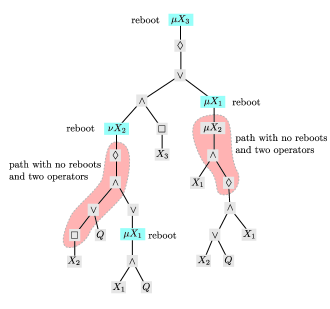
A node $x$ in the syntax tree of a formula that is consistent with $\overline{X}$ is called a reboot if the subformula in the node binds a fixpoint variable $X_{i}$ such that no ancestor of $x$ binds any of the fixpoint variables $\{X_{1},\ldots,X_{i}\}$. The $\overline{X}$-depth of a formula is the biggest number of occurrences of operators from the set $\Box\vphantom{l},\Diamond\vphantom{l},\mu,\nu$ that can be found on a path in the syntax tree that does not visit reboot nodes. The $\overline{X}$-depth is undefined if the formula is not consistent with $\overline{X}$. Figure 1 shows a formula which has $(X_{1},X_{2},X_{3})$-depth 2.

The definition is designed so that $\mu X.\varphi$ and $\varphi[X/\mu X.\varphi]$ have the same $\overline{X}$-depth.

For a set $L\subseteq L_{\mu}$, define the $L$-type of a vertex in a structure to be the set of formulas from $L$ that are true at the vertex. A $\mu$-depth is a pair $\delta=(\overline{X},d)$ where $\overline{X}$ is a sequence of fixpoint variables and $d$ is a natural number. A formula is called consistent with $\delta$ if it is consistent with $\overline{X}$ and its $\overline{X}$-depth is at most $d$. The $\delta$-type of a vertex in a structure is its $L$-type, with $L$ being the set of all formulas consistent with $\delta$. This information is finite thanks to the following lemma.

Lemma 2.3

For every $\mu$-depth $\delta$ and finite set of propositional variables, up to logical equivalence there are finitely many formulas in these propositional variables that are consistent with $\delta$.

Proof 1.

Define the standard depth of a formula to be the biggest number of operators from $\Box\vphantom{l},\Diamond\vphantom{l},\mu,\nu$ on any path in the syntax tree. It is not difficult to see that, when the set of propositional variables is fixed, up to logical equivalence there are finitely many formulas of given standard depth. If $\delta=(\overline{X},d)$ with $\overline{X}=(X_{1},\ldots,X_{n})$, then a formula with $\overline{X}$-depth $d$ has standard depth at most $d\cdot(n+1)$, so the result follows. _■

Although the set in the statement of the above lemma is finite, its size is non-elementary with respect to $\delta$.

2-C Decompositions of Directed Separations

As promised in the introduction, we will prove a decomposition theorem for the union of two structures with a small intersection and some additional edges all going in the same direction. To formalize this, we introduce directed separations.

Definition 2.4

Let $M$ be a $\sigma$-structure. A pair $(M_{1},M_{2})$ of induced substructures is a directed $\sigma$-separation of $M$ with interface $\overline{X}=(x_{1},\ldots,x_{k})$ if

• $V(M)=V(M_{1})\cup V(M_{2})$,

• $X={\left\{x_{1},\ldots,x_{k}\right\}}=V(M_{1})\cap V(M_{2})$,

• and there are no edges from $M_{2}\setminus X$ to $M_{1}\setminus X$.

$\dashv$

Abusing notation, we write $M=(M_{1},M_{2})$ to denote that $(M_{1},M_{2})$ is a directed separation of $M$, and notationally we consider $(M_{1},M_{2})$ to be interchangeable with $M$.

For some $k$, let $\overline{P}=P_{1},\ldots,P_{k}$ be a sequence of fresh proposition symbols. For a $\sigma$-structure $M$ and a $k$-tuple $\overline{X}=(x_{1},\ldots,x_{k})\in V(M)^{k}$, we define $\partial_{\overline{P}}(M,\overline{X})$ to be the $\sigma\cup P$-structure based on $M$ such that $P_{i}$ is true only at the node $x_{i}$. If the sequence $\overline{P}=P_{1},\ldots,P_{k}$ is longer than $\overline{X}=(x_{1},\ldots,x_{l})$, then $\partial_{\overline{P}}(M,\overline{X})$ is defined the same except that $P_{i}$ is always false for $i>l$.

Definition 2.5

Let $(M_{1},M_{2})$, $(M_{1},M_{2}^{\prime})$ be two directed separations with the same interface $\overline{X}$. Let $\overline{P}$ be a set of $\left\lvert X\right\rvert$ many proposition symbols and let $L\subseteq L_{\mu}[\sigma\cup P]$.

We call $(M_{1},M_{2})$, $(M_{1},M_{2}^{\prime})$ $L$-equivalent if

• for every vertex in $X$, its $L$-type is the same in $\partial_{\overline{P}}(M_{2},\overline{X})$ and $\partial_{\overline{P}}(M_{2}^{\prime},\overline{X})$, respectively, and

• for every edge $(v,w)$ in $(M_{1},M_{2})$ with $v\in M_{1},w\in M_{2}$ there is an edge $(v,w^{\prime})$ in $(M_{1},M_{2}^{\prime})$ with $w\in M_{2}^{\prime}$ such that $w$ and $w^{\prime}$ have the same $L$-types in $\partial_{\overline{P}}(M_{2},\overline{X})$ and $\partial_{\overline{P}}(M_{2}^{\prime},\overline{X})$, respectively, and vice versa.

$\dashv$

If $\delta$ is a $\mu$-depth, we say that two directed separations are $\delta$-equivalent if they are $L$-equivalent with $L$ being all formulas consistent with $\delta$. Let us state our main theorem.

Theorem 2.6

Let $\delta$ be a $\mu$-depth, and let $M=(M_{1},M_{2})$, $M^{\prime}=(M_{1},M_{2}^{\prime})$ be $\delta$-equivalent directed separations. Then for every node in $M_{1}$, its $\delta$-type is the same in $M$ and $M^{\prime}$.

In fact, we will prove a more general version of theorem 2.6, without limiting us to $\mu$-depth. It turns out that there exists a suitable closure operator $\mathrm{CL}_{P}:2^{L_{\mu}}\to 2^{L_{\mu}}$ that maps finite sets to finite sets such that the main theorem holds for $\mathrm{CL}_{P}(L)$-equivalent directed separations. In particular, we can choose $L={\left\{\varphi\right\}}$ if we are only interested in the model checking problem for a fixed formula $\varphi$ consistent with $\delta$. Then $\mathrm{CL}_{P}({\left\{\varphi\right\}})$ will be significantly smaller than the set of all $\delta$-consistent formulas.

3 Proof of the Decomposition Theorem

Definition 3.1

For $\varphi\in L_{\mu}$, let $\mathrm{sub}(\varphi)$ be the set of all indexed subformulas without formulas of the form $X$ for fixpoint variables $X$. That is,

$$\mathrm{sub}(\varphi) \mathrel{\mathchoice{\vbox{\hbox{$\displaystyle:$}}}{\vbox{\hbox{$\textstyle:$}}}{\vbox{\hbox{$\scriptstyle:$}}}{\vbox{\hbox{$\scriptscriptstyle:$}}}{=}}\{(\psi,i)\mid\text{$\psi$ is a subformula of $\varphi$ at position $i$}$$

$$\qquad\text{in the string $\varphi$ and $\psi$ is not a variable}\}.$$

Let $\mathrm{sub}^{+}(\varphi)=\mathrm{sub}(\varphi)\setminus{\left\{(\varphi,0)\right\}}$ be the set of proper subformulas.

For an occurrence of a fixpoint variable $X$ in a formula $\varphi$, its definition in $\varphi$ is the enclosing fixpoint $(\mu X.\psi,i)\in\mathrm{sub}(\varphi)$ (or $(\nu X.\psi,i)\in\mathrm{sub}(\varphi)$) where this occurrence of $X$ is quantified. For a formula $(\psi,i)\in\mathrm{sub}(\varphi)$, let $\mathrm{closure}_{\varphi}(\psi,i)=(\psi^{\prime},i)$ be such that $\psi^{\prime}$ is the formula $\psi$ with all free variables replaced by their definitions until there are no more free variables.

Define $\mathrm{CL}(\varphi)\mathrel{\mathchoice{\vbox{\hbox{$\displaystyle:$}}}{\vbox{\hbox{$\textstyle:$}}}{\vbox{\hbox{$\scriptstyle:$}}}{\vbox{\hbox{$\scriptscriptstyle:$}}}{=}}{\left\{\mathrm{closure}_{\varphi}(\psi,i)\mid(\psi,i)\in\mathrm{sub}(\varphi)\right\}}$ and $\mathrm{CL}^{+}(\varphi)=\mathrm{CL}(\varphi)\setminus{\left\{(\varphi,0)\right\}}$. $\dashv$

We will often not distinguish formulas in $\mathrm{sub}(\varphi)$ and $\mathrm{CL}(\varphi)$ and instead identify them via the obvious bijection that preserves the second component.

We will usually write $\psi\in\mathrm{sub}(\varphi)$ instead of $(\psi,i)\in\mathrm{sub}(\varphi)$ if there is no confusion. We only need the index $i$ in order to distinguish identically looking subformulas.

Even though two subformulas may look identical, they could be in the scope of different fixpoint operators. A few paragraphs below we will introduce a closure operation called $\mathrm{PT}_{P}$ that modifies different subformulas in different ways in order to distinguish between these cases. For this reason we need to keep track of the positions of the subformulas. In the rest of the paper, whenever we mention an element of $\mathrm{sub}(\varphi)$ or $\mathrm{CL}(\varphi)$, the reader should assume that it also contains the position of the subformula in $\varphi$.

Lemma 3.2

For all $\varphi\in L_{\mu}$, the set

$$\{\psi\mid(\psi,i)\in\mathrm{CL}(\varphi)\text{ for some $i$}\}$$

is equal to the usual definition of the Fischer-Ladner closure of $\varphi$ (see e.g., [21, Definition 4.1]).

For a set of formulas $L\subseteq L_{\mu}$, define $\mathrm{CL}(L)\mathrel{\mathchoice{\vbox{\hbox{$\displaystyle:$}}}{\vbox{\hbox{$\textstyle:$}}}{\vbox{\hbox{$\scriptstyle:$}}}{\vbox{\hbox{$\scriptscriptstyle:$}}}{=}}\{\psi\mid\text{$\varphi\in L$, $(\psi,i)\in\mathrm{CL}(\varphi)$}\}$. In this set we do not need the index $i$, different from $\mathrm{CL}(\varphi)$.

Let $P={\left\{P_{1},\ldots,P_{k}\right\}}$ be a set of proposition symbols disjoint from $\sigma$.

For a formula $\varphi\in L_{\mu}[\sigma\cup P]$ and $\varphi^{\prime}\in L_{\mu}[\sigma\cup P]$, we call $\varphi^{\prime}$ a priority tracking variant of $\varphi$ if $\varphi^{\prime}$ is syntactically derived from $\varphi$ by applying the following operation for each subformula $\psi$ of the form $\psi=\Diamond\vphantom{l}\chi$ or $\psi=\Box\vphantom{l}\chi$.

1. If $\psi=\Diamond\vphantom{l}\chi$, then pick a set $Q\subseteq P$ and replace the subformula $\psi$ by

   $$\biggl{(}\Bigl{(}\bigvee_{R\in Q}R\Bigr{)}\vee\Diamond\vphantom{l}\chi\biggr{)}.$$

2. If $\psi=\Box\vphantom{l}\chi$, then pick a set $Q\subseteq P$ and replace the subformula $\psi$ by

   $$\biggl{(}\Bigl{(}\bigwedge_{R\in Q}\neg R\Bigr{)}\wedge\Box\vphantom{l}\chi\biggr{)}.$$

We denote the set of all priority tracking variants of $\varphi$ with respect to $P$ by $\mathrm{PT}_{P}(\varphi)$. Note that $\mathrm{PT}_{P}(\varphi)$ is finite because $\varphi$ has a finite number of subformulas and $P$ is a finite set. Similar to $\mathrm{CL}$, we define $\mathrm{PT}_{P}(L)$ for sets of formulas $L\subseteq L_{\mu}[\sigma\cup P]$ as $\mathrm{PT}_{P}(L)\mathrel{\mathchoice{\vbox{\hbox{$\displaystyle:$}}}{\vbox{\hbox{$\textstyle:$}}}{\vbox{\hbox{$\scriptstyle:$}}}{\vbox{\hbox{$\scriptscriptstyle:$}}}{=}}\bigcup_{\varphi\in L}\mathrm{PT}_{P}(\varphi)$.

Definition 3.3

Let $\mathrm{CL}_{P}(L)\mathrel{\mathchoice{\vbox{\hbox{$\displaystyle:$}}}{\vbox{\hbox{$\textstyle:$}}}{\vbox{\hbox{$\scriptstyle:$}}}{\vbox{\hbox{$\scriptscriptstyle:$}}}{=}}\mathrm{PT}_{P}(\mathrm{CL}(L))$. $\dashv$

Lemma 3.4

$\mathrm{CL}_{P}(\mathrm{CL}_{P}(L))=\mathrm{CL}_{P}(L)$ for all $L\subseteq L_{\mu}[\sigma\cup P]$.

Proof 2.

By definition, $\mathrm{CL}_{P}(L)$ is closed under $\mathrm{PT}_{P}$. Hence, it is enough to show $\mathrm{CL}(\mathrm{CL}_{P}(L))=\mathrm{CL}_{P}(L)$. Let $\mu X.\varphi\in\mathrm{CL}_{P}(L)$. We want to show that $\varphi[X/\mu X.\varphi]\in\mathrm{CL}_{P}(L)$, where $\varphi[X/\mu X.\varphi]$ is $\varphi$ with all free occurrences of $X$ replaced by $\mu X.\varphi$. By definition of $\mathrm{PT}_{P}$, there is a $\mu X.\varphi^{\prime}\in\mathrm{CL}(L)$ such that $\varphi$ is priority tracking variant of $\varphi^{\prime}$. Because $\mathrm{CL}(L)$ is essentially equal to the Fischer-Ladner closure of $L$, we have $\varphi^{\prime}[X/\mu X.\varphi^{\prime}]\in\mathrm{CL}(L)$. Since $\varphi$ is a priority tracking variant of $\varphi^{\prime}$, the formula $\varphi[X/\mu X.\varphi]$ is a priority tracking variant of $\varphi^{\prime}[X/\mu X.\varphi^{\prime}]$, hence $\varphi[X/\mu X.\varphi]\in\mathrm{PT}_{P}(\mathrm{CL}(L))$.

The other cases are similar. _■

Definition 3.5

For a structure $M,v$, a $k$-tupel $\overline{X}\in V(M)^{k}$ and a set $L\subseteq L_{\mu}[\sigma\cup P]$ where $\overline{P}$ is sequence of at least $k$ many proposition symbols, we define the $(L,\overline{P})$-type of $v$ in $M,\overline{X}$ as

$$\mathrm{tp}_{L,\overline{P}}(M,v,\overline{X})\mathrel{\mathchoice{\vbox{\hbox{$\displaystyle:$}}}{\vbox{\hbox{$\textstyle:$}}}{\vbox{\hbox{$\scriptstyle:$}}}{\vbox{\hbox{$\scriptscriptstyle:$}}}{=}}{\left\{\varphi\in\mathrm{CL}_{P}(L)\mathrel{}\middle|\mathrel{}\partial_{\overline{P}}(M,\overline{X}),v\models\varphi\right\}}.$$

We also define the set of $(L,\overline{P})$-types realized in a structure,

$$\mathcal{T}_{L,\overline{P}}(M,\overline{X})\mathrel{\mathchoice{\vbox{\hbox{$\displaystyle:$}}}{\vbox{\hbox{$\textstyle:$}}}{\vbox{\hbox{$\scriptstyle:$}}}{\vbox{\hbox{$\scriptscriptstyle:$}}}{=}}{\left\{\mathrm{tp}_{L,\overline{P}}(M,v,\overline{X})\mathrel{}\middle|\mathrel{}v\in V(M)\right\}}.$$

Finally, let $\mathcal{T}_{L}(\overline{P})\mathrel{\mathchoice{\vbox{\hbox{$\displaystyle:$}}}{\vbox{\hbox{$\textstyle:$}}}{\vbox{\hbox{$\scriptstyle:$}}}{\vbox{\hbox{$\scriptscriptstyle:$}}}{=}}2^{\mathrm{CL}_{P}(L)}$ be the set of all candidates for $(L,\overline{P})$-types. $\dashv$

Using the new terminology, let us restate theorem 2.6 in these more general terms.

Theorem 3.6

Let $\overline{P}$ be a sequence of proposition symbols disjoint from $\sigma$, $L\subseteq L_{\mu}[\sigma\cup P]$ and let $(M_{1},M_{2})$, $(M_{1},M_{2}^{\prime})$ be $\mathrm{CL}_{P}(L)$-equivalent directed $\sigma$-separations with interface $\overline{X}$.

Then for all $v\in M_{1}$, we have

$$\mathrm{tp}_{L,\overline{P}}((M_{1},M_{2}),v,\overline{X})=\mathrm{tp}_{L,\overline{P}}((M_{1},M_{2}^{\prime}),v,\overline{X}).$$

It is not difficult to show that if all formulas in $L$ are consistent with a $\mu$-depth $\delta$, then the same is true for $\mathrm{CL}_{P}(L)$ (this is lemma 3.8). Therefore, $\delta$-equivalence implies $\mathrm{CL}_{P}(L)$-equivalence, and thus theorem 2.6 follows from theorem 3.6. We will also use a different and slightly stronger way of stating theorem 3.6, stated below.

Theorem 3.7

Let $\overline{P}$, $\overline{Q}$ be sequences of proposition symbols such that $\sigma\cap P=\sigma\cap Q=P\cap Q=\emptyset$.

Let $L\subseteq L_{\mu}[\sigma\cup P]$ and $M$ be a structure with a directed $\sigma$-separation $(M_{1},M_{2})$ with interface $\overline{X}$. Let $\overline{Y}\in V(M_{1})^{\left\lvert Q\right\rvert}$ be a tuple.

For all $v\in M_{1}$, the set $\mathrm{tp}_{L,\overline{Q}}(M,v,\overline{Y})$ depends only on

• $M_{1}$ and $\overline{Q}$ and

• ${\left\{(x_{i},\mathrm{tp}_{L,\overline{P}}(M_{2},x_{i},\overline{X}))\mathrel{}\middle|\mathrel{}x_{i}\in X\right\}}$ and

• ${\left\{(v,\mathrm{tp}_{L,\overline{P}}(M_{2},w,\overline{X}))\mid\text{$(v,w)\in E(M)\cap(M_{1}\times M_{2})$}\right\}}$.

Provided $L$ is finite, $\mathrm{tp}_{L,\overline{Q}}(M,v,\overline{Y})$ can be computed from these sets.

Furthermore, for every $w\in M_{2}$, the set $\mathrm{tp}_{L,\overline{Q}}(M,w,\overline{Y})$ depends only on the above sets and on $\mathrm{tp}_{L,\overline{P}}(M_{2},w,\overline{X})$ and can be computed from these sets if $L$ is finite.

3-A Parity Games

To prove the decomposition theorems, we want to use the model checking game of the modal $\mu$-calculus. Instead of replacing a substructure by a different substructure preserving the types in the whole structure, we replace a subgame by a different subgame preserving the winner in the whole game.

For this, we first need parity games, strategies and the model checking game. These are all well-known concepts in the literature, see for example [10]. We briefly review the key concepts.

The winner of a parity game from a given node is always determined. However, in order to replace subgames by different subgames preserving the winner in the whole game, we need a more subtle analysis of the subgame than just its winner.

We call the intersection between a subgame and the rest of the game its interface. For the more subtle analysis, we look at partial strategies, which may be undefined on some nodes of the interface. If a partial strategy is undefined on some node, the player indicates that she would like to leave the subgame. These strategies can be partially ordered by their profiles, that is, the set of interface nodes that are possibly reachable by Player $\Box$, together with the worst priority that Player $\Box$ can enforce.

All this culminates in a proof that the feasibility of profiles of strategies is in fact definable in $L_{\mu}$. The formulas that define profiles in a partial model checking game of $\varphi$ will all be in $\mathrm{CL}_{P}({\left\{\varphi\right\}})$, so this proves that $\mathrm{tp}_{{\left\{\varphi\right\}},\overline{P}}(M,v,\overline{X})$ determines the set of possible profiles, which we will use to define a specific parity game.

Let $\overline{Z}=(Z_{1},\ldots,Z_{n})$ be a finite sequence of fixpoint variables. Recall the definition of a formula consistent with $\overline{Z}$ (definition 2.2 on definition 2.2). We strengthen this definition in the sense that every $Z_{i}$ is either bound only in $\mu$-subformulas or only in $\nu$-subformulas. Let $(p_{1},\ldots,p_{n})$ be a strictly increasing sequence of natural numbers such that $p_{i}$ is odd if and only if $Z_{i}$ is only bound in $\mu$-subformulas.

Let $\varphi\in L_{\mu}$ be consistent with $\overline{Z}$ and $\mu Z_{i}.\psi\in\mathrm{sub}(\varphi)$. We write $\overset{p_{i}}{\mu}Z_{i}.\psi$ to indicate that $Z_{i}$ gets the priority $p_{i}$ in the model checking game that we will define shortly (similarly for $\nu$). We call a formula with numbers over their fixpoint operators an annotated formula. In this section it does not affect the results if the sequences are infinite.

From now on, let us fix a sequence $\overline{Z}$ and a corresponding priority sequence $(p_{1},\ldots,p_{n})$. All formulas in the rest of this section should be consistent with $\overline{Z}$ and annotated with the $p_{i}$, even if we do not mention this explicitly. For example, a formula $\nu Y.\Diamond\vphantom{l}(\mu X.\nu Y.\Diamond\vphantom{l}X\vee\Diamond\vphantom{l}Y)\vee\Diamond\vphantom{l}Y$ consistent with $(X,Y)$ under the priority sequence $(1,2)$ would be labelled as $\overset{2}{\nu}Y.\Diamond\vphantom{l}(\overset{1}{\mu}X.\overset{2}{\nu}Y.\Diamond\vphantom{l}X\vee\Diamond\vphantom{l}Y)\vee\Diamond\vphantom{l}Y$. Note that it cannot be labelled $\overset{2}{\nu}Y.\Diamond\vphantom{l}(\overset{3}{\mu}X.\overset{4}{\nu}Y.\Diamond\vphantom{l}X\vee\Diamond\vphantom{l}Y)\vee\Diamond\vphantom{l}Y$, even though these priorities would work in the model-checking game. However, they violate the sequence $(X,Y)$ and the priority sequence $(1,2)$.

Note that the first formula is an element of $\mathrm{CL}(\overset{1}{\mu}X.\penalty 0\overset{2}{\nu}Y.\Diamond\vphantom{l}X\vee\Diamond\vphantom{l}Y)$. This holds true in general.

Lemma 3.8

Let $\overline{Z}=(Z_{1},\ldots,Z_{n})$, $\varphi\in L_{\mu}$ be consistent with $\overline{Z}$ and $\psi\in\mathrm{CL}(\varphi)$. Then $\psi$ is consistent with $\overline{Z}$.

Proof 3.

We prove this by structural induction. If $\varphi=\chi_{1}\wedge\chi_{2}$, then obviously $\chi_{1}$ and $\chi_{2}$ are consistent with $\overline{Z}$. The same is true for most other cases. The only interesting cases are the fixpoints. We only consider the case of $\mu$ fixed points, the other cases follow analogously.

Assume that $\varphi=\mu Z_{i}.\psi$. We need to show that $\psi[Z_{i}/\varphi]$ is consistent with $\overline{Z}$. Because $\varphi$ is consistent with $\overline{Z}$, the only places where $\psi[X/\varphi]$ could become inconsistent is a subformula of the form $\varphi$ inside the scope of another fixpoint operator $\mu Z_{j}.\chi$ with $j>i$ with $Z_{j}$ being free in $\varphi$. This is impossible because $\varphi$ does not have free variables. _■

Now let us briefly review the definitions of parity games, strategies and model checking games.

Definition 3.9

A parity game $P=(V,V_{\Diamond},E,\omega)$ is a directed graph $(V,E)$ with $V_{\Diamond}\subseteq V$ and a function $\omega:V\to\mathbb{N}$ mapping nodes to priorities. $\dashv$

A parity game is played by two players, Player $\Diamond$ and Player $\Box$. The game starts on a node $v$. It is Player $\Diamond$’s turn if the current node is in $V_{\Diamond}$, otherwise it is Player $\Box$’s turn. In their turn, the players must choose an outgoing edge and the endpoint becomes the current node for the next turn. If a player cannot make a move, he loses. Otherwise, the game continues indefinitely.

The set of nodes visited during an infinite play is an infinite path $\overline{v}=v_{1},v_{2},\ldots$. Let $p$ be the minimum priority that occurs infinitely often on $\overline{v}$. The path $\overline{v}$ is winning for Player $\Diamond$ if and only if $p$ is even.

Definition 3.10

Let $P$ be a parity game. For a partial function $\pi:V(P)^{+}\to V(P)$ on finite non-empty paths of nodes and a path $(v_{1},\ldots,v_{n})\in V(P)^{+}$, we say that $\overline{v}$ is $\pi$-conforming if for all $i<n$ with $v_{i}\in V_{\Diamond}\vphantom{l}(P)$, we have $(v_{1},\ldots,v_{i})\in\operatorname{dom}(\pi)$ and $(v_{i},\pi((v_{1},\ldots,v_{i})))\in E(P)$. An infinite path is $\pi$-conforming if all its initial segments are $\pi$-conforming.

A strategy for Player $\Diamond$ for a game $(P,v_{1})$ is a partial function $\pi:V(P)^{+}\to V(P)$ with the following conditions.

1. For every $(v_{1},\ldots,v_{n})\in\operatorname{dom}(\pi)$, the sequence $(v_{1},\ldots,\penalty 0v_{n},\pi(v_{1},\ldots,v_{n}))$ is a $\pi$-conforming path in $P$ with $v_{n}\in V_{\Diamond}\vphantom{l}(P)$.

2. For every $\pi$-conforming path $(v_{1},\ldots,v_{n})$, if $v_{n}\in V_{\Diamond}\vphantom{l}(P)$, then $(v_{1},\ldots,v_{n})\in\operatorname{dom}(\pi)$.

A strategy $\pi$ is winning for Player $\Diamond$ if every maximal $\pi$-conforming path is winning for Player $\Diamond$. A game $P$ on a node $v$ is winning for Player $\Diamond$ if Player $\Diamond$ has a winning strategy for $(P,v)$. $\dashv$

Definition 3.11

A strategy $\pi$ is positional if $\pi(v_{1},\ldots,v_{n})$ only depends on $v_{n}$. $\dashv$

When we talk about strategies and do not explicitly mention the player, we assume that the strategy is meant for Player $\Diamond$. The following result is well-known (see e.g., [23]).

Theorem 3.12

For every winning strategy $\pi$ for a game $(P,v)$, there exists a positional winning strategy $\rho$ for $(P,v)$.

Parity games are relevant because they are the model checking game for the modal $\mu$-calculus.

Definition 3.13

For a $\sigma$-structure $M$ and a formula $\varphi\in L_{\mu}[\sigma]$, let $\mathrm{P}[M,\varphi]=(V,V_{\Diamond}\vphantom{l},E,\omega)$ be the model checking game defined as follows.

$$V(\mathrm{P}[M,\varphi]) \mathrel{\mathchoice{\vbox{\hbox{$\displaystyle:$}}}{\vbox{\hbox{$\textstyle:$}}}{\vbox{\hbox{$\scriptstyle:$}}}{\vbox{\hbox{$\scriptscriptstyle:$}}}{=}}M\times\mathrm{CL}(\varphi)$$

There is a an edge from $(v,\psi)$ to $(w,\chi)$ if

• $v=w$ and $\psi\in{\left\{\chi\wedge\chi^{\prime},\chi\vee\chi^{\prime},\chi^{\prime}\wedge\chi,\chi^{\prime}\vee\chi\right\}}$ for some $\chi^{\prime}$ or

• $v=w$, $\psi\in{\left\{\mu X.\chi^{\prime},\nu X.\chi^{\prime}\right\}}$ and $\chi=\mathrm{closure}_{\varphi}(\chi^{\prime})$ or

• $(v,w)\in E(M)$ and $\psi\in{\left\{\Diamond\vphantom{l}\psi,\Box\vphantom{l}\psi\right\}}$.

A node $(v,\psi)$ is a $\Box\vphantom{l}$-node if either

• $\psi=P$ and $M,v\models P$ or

• $\psi\in{\left\{\chi\wedge\chi^{\prime},\Box\vphantom{l}\chi\right\}}$ for some $\chi,\chi^{\prime}$.

A node $(v,\psi)$ has the priority

$$\omega(v,\psi) \mathrel{\mathchoice{\vbox{\hbox{$\displaystyle:$}}}{\vbox{\hbox{$\textstyle:$}}}{\vbox{\hbox{$\scriptstyle:$}}}{\vbox{\hbox{$\scriptscriptstyle:$}}}{=}}\begin{cases}p&\text{if $\psi=\overset{p}{\mu}X.\chi$ or $\psi=\overset{p}{\nu}X.\chi$ for some $\chi$}\\ p^{\prime}&\text{otherwise},\end{cases}$$

where $p^{\prime}$ is the maximum priority. $\dashv$

It is easy to show that this definition gives a well-defined model checking game (see e.g., [22]).

3-B Profiles and Types

In the previous section we considered parity games, (positional) strategies and the model checking game. We now generalize these definition to partial games and partial strategies. This is necessary so we can analyze the effect of replacing a subgame by a different, but in some sense similar subgame.

Definition 3.14

A partial parity game is a parity game $P$ with a subset $U\subseteq V(P)$ called the interface. $\dashv$

The game is played the same way as a parity game, except that upon reaching an interface $\Diamond$-node, Player $\Diamond$ may choose to end the play and win immediately. Therefore, a partial strategy for Player $\Diamond$ is defined the same way as in a non-partial parity game, except that the partial strategy may be undefined on plays that end in an interface $\Diamond$-node.

Definition 3.15

Let $P$ be a partial parity game. A partial strategy for Player $\Diamond$ for a game $(P,v_{1})$ is a partial function $\pi:V(P)^{+}\to V(P)$ with the following conditions.

1. For every $(v_{1},\ldots,v_{n})\in\operatorname{dom}(\pi)$, the sequence $(v_{1},\ldots,\penalty 0v_{n},\pi(v_{1},\ldots,v_{n}))$ is a $\pi$-conforming path in $P$ with $v_{n}\in V_{\Diamond}\vphantom{l}(P)$.

2. For every $\pi$-conforming path $(v_{1},\ldots,v_{n})$, if $v_{n}\in V_{\Diamond}\vphantom{l}(P)$ and $v_{n}\notin U$, then $(v_{1},\ldots,v_{n})\in\operatorname{dom}(\pi)$.

$\dashv$

A partial strategy $\pi$ is called winning if for every strategy of the opponent, the resulting play either visits an interface node where $\pi$ is undefined or satisfies the parity condition. Formally, we define this as follows.

Definition 3.16

Let $(P,v_{1})$ be a partial parity game with interface $U$ and $\pi$ be a partial strategy. Let $P^{\prime}$ be the game constructed from $P$ by adding a $\Box\vphantom{l}$-node called $\top$ and an edge from every node in $V_{\Diamond}\vphantom{l}\cap U$ to $\top$. Then define $\pi^{\prime}$ as an extension of $\pi$ such that on all $\pi$-conforming paths $(v_{1},\ldots,v_{n})$ with $v_{n}\in V_{\Diamond}\vphantom{l}\cap U$, if $(v_{1},\ldots,v_{n})\notin\operatorname{dom}(\pi)$, then $\pi^{\prime}((v_{1},\ldots,v_{n}))=\top$. Then $\pi^{\prime}$ is a strategy on $(P^{\prime},v_{1})$.

We say that $\pi$ is a partial winning strategy from node $v_{1}$ iff $\pi^{\prime}$ wins from node $v_{1}$ in the game $P^{\prime}$. $\dashv$

If we have a structure together with some subset of its nodes, we consider the corresponding model checking games to be partial with respect to these nodes.

Definition 3.17

Let $\varphi\in L_{\mu}[\sigma]$, $M$ be a $\sigma$-structure and $X\subseteq V(M)$. The game $\mathrm{P}[X,M,\varphi]$ is the partial parity game defined as $\mathrm{P}[M,\varphi]$ with interface $\{(v,\psi)\in X\times\mathrm{CL}(\varphi)\mid\text{$\psi$ starts with $\Diamond\vphantom{l}$ or $\Box\vphantom{l}$}\}$. We will usually write $\mathrm{P}[M,\varphi]$ for this game if $X$ is clear from the context. $\dashv$

We emphasize again that $\mathrm{P}[X,M,\varphi]$ and $\mathrm{P}[M,\varphi,$] are exactly the same game, only viewed from two different angles.

Definition 3.18

Let $P$ be a partial parity game with interface $U$. We define

$$\mathrm{\text{strategy-targets}}(P)\mathrel{\mathchoice{\vbox{\hbox{$\displaystyle:$}}}{\vbox{\hbox{$\textstyle:$}}}{\vbox{\hbox{$\scriptstyle:$}}}{\vbox{\hbox{$\scriptscriptstyle:$}}}{=}}{\left\{(u,p)\mathrel{}\middle|\mathrel{}\text{$u\in U$, $p$ a priority of $P$}\right\}}$$

$$\mathrm{profiles}(P)\mathrel{\mathchoice{\vbox{\hbox{$\displaystyle:$}}}{\vbox{\hbox{$\textstyle:$}}}{\vbox{\hbox{$\scriptstyle:$}}}{\vbox{\hbox{$\scriptscriptstyle:$}}}{=}}\{y\subseteq\mathrm{\text{strategy-targets}}(P)\mid{}\text{for all $u$}$$

$$\hskip 68.28644pt\text{there is at most one $p$ with $(u,p)\in y$}\}.$$

$\dashv$

Definition 3.19

Let $\sqsubseteq$ be the reward ordering on priorities. That is, $p\sqsubseteq p^{\prime}$ if $p$ is better for Player $\Diamond$ than $p^{\prime}$. Formally, $p\sqsubseteq p^{\prime}$ is true if and only if

• $p$ is even and $p^{\prime}$ is odd or

• both $p$ and $p^{\prime}$ are even and $p\leq p^{\prime}$ or

• both $p$ and $p^{\prime}$ are odd and $p\geq p^{\prime}$.

$\dashv$

Definition 3.20

Let $P$ be a partial parity game with interface $U$, $v_{1}\in V(P)$ and let $\pi$ be a partial winning strategy for $(P,v_{1})$. We define

$$\mathrm{preprofile}(\pi,v_{1}) \mathrel{\mathchoice{\vbox{\hbox{$\displaystyle:$}}}{\vbox{\hbox{$\textstyle:$}}}{\vbox{\hbox{$\scriptstyle:$}}}{\vbox{\hbox{$\scriptscriptstyle:$}}}{=}}\{(v_{n},\min_{1\leq i\leq n}\omega(v_{i}))\mid$$

$$n>1 (v_{1},\ldots,v_{n})$$, is a path with

$$\hskip 21.33955pt\text{$v_{n}\in U$ and $(v_{1},\ldots,v_{n})\notin\operatorname{dom}(\pi)$}\}$$

$$\mathrm{profile}(\pi,v_{1}) \mathrel{\mathchoice{\vbox{\hbox{$\displaystyle:$}}}{\vbox{\hbox{$\textstyle:$}}}{\vbox{\hbox{$\scriptstyle:$}}}{\vbox{\hbox{$\scriptscriptstyle:$}}}{=}}\{(u,p)\mid\text{$p$ is $\sqsubseteq$-maximal such that}$$

$$\hskip 21.33955pt\text{$(u,p)\in\mathrm{preprofile}(\pi,v_{1})$}\}.$$

The $\min$ is taken with respect to the usual ordering $\leq$.

We say that a profile $y\in\mathrm{profiles}(P)$ is possible on $(P,v_{1})$ if there exists a $\pi$ such that $y=\mathrm{profile}(\pi,v_{1})$. $\dashv$

Definition 3.21

Let $y,y^{\prime}\in\mathrm{profiles}(P)$. We say that $y$ is at least as good as $y^{\prime}$ iff for every $(u,p)\in y$, there is a $(u,p^{\prime})\in y^{\prime}$ with $p\sqsubseteq p^{\prime}$. We denote this as $y\sqsubseteq y^{\prime}$. $\dashv$

Figure 2:

As an example, consider the two parity games given in fig. 2 with interface nodes , . For simplicity, we assume that all nodes in these parity games have priority 0. Then the profile ${\left\{(\leavevmode\hbox to7.87pt{\vbox to7.87pt{\pgfpicture\makeatletter\hbox{\hskip 3.93588pt\lower-3.93588pt\hbox to0.0pt{\pgfsys@beginscope\pgfsys@invoke{ }\definecolor{pgfstrokecolor}{rgb}{0,0,0}\pgfsys@color@rgb@stroke{0}{0}{0}\pgfsys@invoke{ }\pgfsys@color@rgb@fill{0}{0}{0}\pgfsys@invoke{ }\pgfsys@setlinewidth{0.4pt}\pgfsys@invoke{ }\nullfont\pgfsys@beginscope\pgfsys@invoke{ }\pgfsys@invoke{\lxSVG@closescope }\pgfsys@endscope\hbox to0.0pt{\pgfsys@beginscope\pgfsys@invoke{ }{{}}\pgfsys@beginscope\pgfsys@invoke{ }\pgfsys@setlinewidth{0.8pt}\pgfsys@invoke{ }\pgfsys@setlinewidth{1.0pt}\pgfsys@invoke{ }\hbox{\hbox{{\pgfsys@beginscope\pgfsys@invoke{ }\definecolor[named]{pgfstrokecolor}{rgb}{0,0,0}\pgfsys@color@gray@stroke{0}\pgfsys@invoke{ }\definecolor[named]{pgffillcolor}{rgb}{0,0,0}\pgfsys@color@gray@fill{0}\pgfsys@invoke{ }\pgfsys@setlinewidth{0.8pt}\pgfsys@invoke{ }\definecolor[named]{pgffillcolor}{rgb}{1,1,1}\pgfsys@color@gray@fill{1}\pgfsys@invoke{ }\pgfsys@setlinewidth{0.8pt}\pgfsys@invoke{ }{{}{{{}}}{{}}{}{}{}{}{}{}{}{}{}{\pgfsys@beginscope\pgfsys@invoke{ }\definecolor[named]{pgfstrokecolor}{rgb}{0,0,0}\pgfsys@color@gray@stroke{0}\pgfsys@invoke{ }\definecolor[named]{pgffillcolor}{rgb}{0,0,0}\pgfsys@color@gray@fill{0}\pgfsys@invoke{ }\pgfsys@setlinewidth{0.8pt}\pgfsys@invoke{ }\definecolor[named]{pgffillcolor}{rgb}{1,1,1}\pgfsys@color@gray@fill{1}\pgfsys@invoke{ }\pgfsys@setlinewidth{0.8pt}\pgfsys@invoke{ }{}\pgfsys@moveto{3.53589pt}{0.0pt}\pgfsys@curveto{3.53589pt}{1.95284pt}{1.95284pt}{3.53589pt}{0.0pt}{3.53589pt}\pgfsys@curveto{-1.95284pt}{3.53589pt}{-3.53589pt}{1.95284pt}{-3.53589pt}{0.0pt}\pgfsys@curveto{-3.53589pt}{-1.95284pt}{-1.95284pt}{-3.53589pt}{0.0pt}{-3.53589pt}\pgfsys@curveto{1.95284pt}{-3.53589pt}{3.53589pt}{-1.95284pt}{3.53589pt}{0.0pt}\pgfsys@closepath\pgfsys@moveto{0.0pt}{0.0pt}\pgfsys@fillstroke\pgfsys@invoke{ } \pgfsys@invoke{\lxSVG@closescope }\pgfsys@endscope}{{{{}}\pgfsys@beginscope\pgfsys@invoke{ }\pgfsys@transformcm{1.0}{0.0}{0.0}{1.0}{0.0pt}{0.0pt}\pgfsys@invoke{ }\hbox{{\definecolor{pgfstrokecolor}{rgb}{0,0,0}\pgfsys@color@rgb@stroke{0}{0}{0}\pgfsys@invoke{ }\pgfsys@color@rgb@fill{0}{0}{0}\pgfsys@invoke{ }\hbox{} }}\pgfsys@invoke{\lxSVG@closescope }\pgfsys@endscope}}} \pgfsys@invoke{\lxSVG@closescope }\pgfsys@endscope}}} \pgfsys@invoke{\lxSVG@closescope }\pgfsys@endscope \pgfsys@invoke{\lxSVG@closescope }\pgfsys@endscope{}{}{}\hss}\pgfsys@discardpath\pgfsys@invoke{\lxSVG@closescope }\pgfsys@endscope\hss}}\lxSVG@closescope\endpgfpicture}},0)\right\}}$ is possible on $(P_{1},v)$ but not on $(P_{2},v)$. On the other hand, the profile ${\left\{(\leavevmode\hbox to7.87pt{\vbox to7.87pt{\pgfpicture\makeatletter\hbox{\hskip 3.93588pt\lower-3.93588pt\hbox to0.0pt{\pgfsys@beginscope\pgfsys@invoke{ }\definecolor{pgfstrokecolor}{rgb}{0,0,0}\pgfsys@color@rgb@stroke{0}{0}{0}\pgfsys@invoke{ }\pgfsys@color@rgb@fill{0}{0}{0}\pgfsys@invoke{ }\pgfsys@setlinewidth{0.4pt}\pgfsys@invoke{ }\nullfont\pgfsys@beginscope\pgfsys@invoke{ }\pgfsys@invoke{\lxSVG@closescope }\pgfsys@endscope\hbox to0.0pt{\pgfsys@beginscope\pgfsys@invoke{ }{{}}\pgfsys@beginscope\pgfsys@invoke{ }\pgfsys@setlinewidth{0.8pt}\pgfsys@invoke{ }\pgfsys@setlinewidth{1.0pt}\pgfsys@invoke{ }\hbox{\hbox{{\pgfsys@beginscope\pgfsys@invoke{ }\definecolor[named]{pgfstrokecolor}{rgb}{0,0,0}\pgfsys@color@gray@stroke{0}\pgfsys@invoke{ }\definecolor[named]{pgffillcolor}{rgb}{0,0,0}\pgfsys@color@gray@fill{0}\pgfsys@invoke{ }\pgfsys@setlinewidth{0.8pt}\pgfsys@invoke{ }\definecolor[named]{pgffillcolor}{rgb}{1,1,1}\pgfsys@color@gray@fill{1}\pgfsys@invoke{ }\pgfsys@setlinewidth{0.8pt}\pgfsys@invoke{ }{{}{{{}}}{{}}{}{}{}{}{}{}{}{}{}{\pgfsys@beginscope\pgfsys@invoke{ }\definecolor[named]{pgfstrokecolor}{rgb}{0,0,0}\pgfsys@color@gray@stroke{0}\pgfsys@invoke{ }\definecolor[named]{pgffillcolor}{rgb}{0,0,0}\pgfsys@color@gray@fill{0}\pgfsys@invoke{ }\pgfsys@setlinewidth{0.8pt}\pgfsys@invoke{ }\definecolor[named]{pgffillcolor}{rgb}{1,1,1}\pgfsys@color@gray@fill{1}\pgfsys@invoke{ }\pgfsys@setlinewidth{0.8pt}\pgfsys@invoke{ }{}\pgfsys@moveto{3.53589pt}{0.0pt}\pgfsys@curveto{3.53589pt}{1.95284pt}{1.95284pt}{3.53589pt}{0.0pt}{3.53589pt}\pgfsys@curveto{-1.95284pt}{3.53589pt}{-3.53589pt}{1.95284pt}{-3.53589pt}{0.0pt}\pgfsys@curveto{-3.53589pt}{-1.95284pt}{-1.95284pt}{-3.53589pt}{0.0pt}{-3.53589pt}\pgfsys@curveto{1.95284pt}{-3.53589pt}{3.53589pt}{-1.95284pt}{3.53589pt}{0.0pt}\pgfsys@closepath\pgfsys@moveto{0.0pt}{0.0pt}\pgfsys@fillstroke\pgfsys@invoke{ } \pgfsys@invoke{\lxSVG@closescope }\pgfsys@endscope}{{{{}}\pgfsys@beginscope\pgfsys@invoke{ }\pgfsys@transformcm{1.0}{0.0}{0.0}{1.0}{0.0pt}{0.0pt}\pgfsys@invoke{ }\hbox{{\definecolor{pgfstrokecolor}{rgb}{0,0,0}\pgfsys@color@rgb@stroke{0}{0}{0}\pgfsys@invoke{ }\pgfsys@color@rgb@fill{0}{0}{0}\pgfsys@invoke{ }\hbox{} }}\pgfsys@invoke{\lxSVG@closescope }\pgfsys@endscope}}} \pgfsys@invoke{\lxSVG@closescope }\pgfsys@endscope}}} \pgfsys@invoke{\lxSVG@closescope }\pgfsys@endscope \pgfsys@invoke{\lxSVG@closescope }\pgfsys@endscope{}{}{}\hss}\pgfsys@discardpath\pgfsys@invoke{\lxSVG@closescope }\pgfsys@endscope\hss}}\lxSVG@closescope\endpgfpicture}},0),(\leavevmode\hbox to7.87pt{\vbox to7.87pt{\pgfpicture\makeatletter\hbox{\hskip 3.93588pt\lower-3.93588pt\hbox to0.0pt{\pgfsys@beginscope\pgfsys@invoke{ }\definecolor{pgfstrokecolor}{rgb}{0,0,0}\pgfsys@color@rgb@stroke{0}{0}{0}\pgfsys@invoke{ }\pgfsys@color@rgb@fill{0}{0}{0}\pgfsys@invoke{ }\pgfsys@setlinewidth{0.4pt}\pgfsys@invoke{ }\nullfont\pgfsys@beginscope\pgfsys@invoke{ }\pgfsys@invoke{\lxSVG@closescope }\pgfsys@endscope\hbox to0.0pt{\pgfsys@beginscope\pgfsys@invoke{ }{{}}\pgfsys@beginscope\pgfsys@invoke{ }\pgfsys@setlinewidth{0.8pt}\pgfsys@invoke{ }\pgfsys@setlinewidth{1.0pt}\pgfsys@invoke{ }\hbox{\hbox{{\pgfsys@beginscope\pgfsys@invoke{ }\definecolor[named]{pgfstrokecolor}{rgb}{0,0,0}\pgfsys@color@gray@stroke{0}\pgfsys@invoke{ }\definecolor[named]{pgffillcolor}{rgb}{0,0,0}\pgfsys@color@gray@fill{0}\pgfsys@invoke{ }\pgfsys@setlinewidth{0.8pt}\pgfsys@invoke{ }\definecolor{pgffillcolor}{rgb}{0.7,0.7,0.7}\pgfsys@color@gray@fill{0.7}\pgfsys@invoke{ }{{}{{{}}}{{}}{}{}{}{}{}{}{}{}{}{\pgfsys@beginscope\pgfsys@invoke{ }\definecolor[named]{pgfstrokecolor}{rgb}{0,0,0}\pgfsys@color@gray@stroke{0}\pgfsys@invoke{ }\definecolor[named]{pgffillcolor}{rgb}{0,0,0}\pgfsys@color@gray@fill{0}\pgfsys@invoke{ }\pgfsys@setlinewidth{0.8pt}\pgfsys@invoke{ }\definecolor{pgffillcolor}{rgb}{0.7,0.7,0.7}\pgfsys@color@gray@fill{0.7}\pgfsys@invoke{ }{}\pgfsys@moveto{3.53589pt}{0.0pt}\pgfsys@curveto{3.53589pt}{1.95284pt}{1.95284pt}{3.53589pt}{0.0pt}{3.53589pt}\pgfsys@curveto{-1.95284pt}{3.53589pt}{-3.53589pt}{1.95284pt}{-3.53589pt}{0.0pt}\pgfsys@curveto{-3.53589pt}{-1.95284pt}{-1.95284pt}{-3.53589pt}{0.0pt}{-3.53589pt}\pgfsys@curveto{1.95284pt}{-3.53589pt}{3.53589pt}{-1.95284pt}{3.53589pt}{0.0pt}\pgfsys@closepath\pgfsys@moveto{0.0pt}{0.0pt}\pgfsys@fillstroke\pgfsys@invoke{ } \pgfsys@invoke{\lxSVG@closescope }\pgfsys@endscope}{{{{}}\pgfsys@beginscope\pgfsys@invoke{ }\pgfsys@transformcm{1.0}{0.0}{0.0}{1.0}{0.0pt}{0.0pt}\pgfsys@invoke{ }\hbox{{\definecolor{pgfstrokecolor}{rgb}{0,0,0}\pgfsys@color@rgb@stroke{0}{0}{0}\pgfsys@invoke{ }\pgfsys@color@rgb@fill{0}{0}{0}\pgfsys@invoke{ }\hbox{} }}\pgfsys@invoke{\lxSVG@closescope }\pgfsys@endscope}}} \pgfsys@invoke{\lxSVG@closescope }\pgfsys@endscope}}} \pgfsys@invoke{\lxSVG@closescope }\pgfsys@endscope \pgfsys@invoke{\lxSVG@closescope }\pgfsys@endscope{}{}{}\hss}\pgfsys@discardpath\pgfsys@invoke{\lxSVG@closescope }\pgfsys@endscope\hss}}\lxSVG@closescope\endpgfpicture}},0)\right\}}$ is possible on both $(P_{1},v)$ and $(P_{2},v)$. Note that on $(P_{1},v)$, the last profile is only possible with a non-positional strategy. However, the need for a non-positional strategy here is of course somewhat artificial because Player $\Diamond$ must deliberately avoid a decision where she could simply make one.

As one might expect, every partial strategy can be converted into a positional partial strategy at least as good as the original strategy.

Lemma 3.22

Let $P=(V,V_{\Diamond}\vphantom{l},E,\omega)$ be a partial parity game with interface $U$, $v\in V$ and $\pi$ be a partial strategy for $(P,v)$. Then there exists a positional partial strategy $\rho$ such that $\mathrm{profile}(\rho,v)\sqsubseteq\mathrm{profile}(\pi,v)$.

Proof 4.

The proof is a reduction to the positional determinacy of (non-partial) parity games.

We define a game $P^{\prime}=(V^{\prime},V_{\Diamond}\vphantom{l}^{\prime},E^{\prime},\omega^{\prime})$ based on $P$ and use theorem 3.12. Let

$$V^{\prime} \mathrel{\mathchoice{\vbox{\hbox{$\displaystyle:$}}}{\vbox{\hbox{$\textstyle:$}}}{\vbox{\hbox{$\scriptstyle:$}}}{\vbox{\hbox{$\scriptscriptstyle:$}}}{=}}V\cup{\left\{v_{p}\mathrel{}\middle|\mathrel{}\text{$p$ is a priority of $P$}\right\}}\cup{\left\{v_{\bot}\right\}}$$

$$V_{\Diamond}\vphantom{l}^{\prime} \mathrel{\mathchoice{\vbox{\hbox{$\displaystyle:$}}}{\vbox{\hbox{$\textstyle:$}}}{\vbox{\hbox{$\scriptstyle:$}}}{\vbox{\hbox{$\scriptscriptstyle:$}}}{=}}V_{\Diamond}\vphantom{l}\cup{\left\{v_{\bot}\right\}}$$

$$E^{\prime} \mathrel{\mathchoice{\vbox{\hbox{$\displaystyle:$}}}{\vbox{\hbox{$\textstyle:$}}}{\vbox{\hbox{$\scriptstyle:$}}}{\vbox{\hbox{$\scriptscriptstyle:$}}}{=}}E\cup{\left\{(v_{p},v)\mathrel{}\middle|\mathrel{}\text{$p$ is a priority of $P$}\right\}}\cup{}$$

$${\left\{(u,v_{p})\mathrel{}\middle|\mathrel{}\text{$p$ is odd and $(u,p-1)\in\mathrm{profile}(\pi,v)$}\right\}}\cup{}$$

$${\left\{(u,v_{p})\mathrel{}\middle|\mathrel{}\text{$p$ is even and $(u,p+1)\in\mathrm{profile}(\pi,v)$}\right\}}\cup{}$$

$${\left\{(u,v_{\bot})\mathrel{}\middle|\mathrel{}\text{$(u,p)\notin\mathrm{profile}(\pi,v)$ for all $p$}\right\}}$$

$$\omega^{\prime}(w) \mathrel{\mathchoice{\vbox{\hbox{$\displaystyle:$}}}{\vbox{\hbox{$\textstyle:$}}}{\vbox{\hbox{$\scriptstyle:$}}}{\vbox{\hbox{$\scriptscriptstyle:$}}}{=}}\begin{cases}\omega(w)&\text{if $w\in V(P)$}\\ 0&\text{if $w=v_{\bot}$}\\ p&\text{if $w=v_{p}$}.\end{cases}$$

Note that for each $u\in U$, there is exactly one $v_{p}$ such that $(u,v_{p})\in E^{\prime}$. So we can extend $\pi$ to a strategy $\pi^{\prime}$ on $P^{\prime}$ by defining $\pi^{\prime}(v_{1},\ldots,u)=v_{p}$ if $\pi(v_{1},\ldots,u)$ is undefined.

We claim that $\pi^{\prime}$ is a winning strategy. Let $v=v_{1},v_{2},\ldots$ be an infinite $\pi^{\prime}$-conforming path. Clearly the path is winning if it has a $\pi$-conforming suffix.

So assume that it visits some $u\in U$ an infinite number of times followed by $v_{p}$. If $p$ is odd, then $(u,p-1)\in\mathrm{profile}(\pi,v)$ guarantees that the worst priority on all path segments that go from $v$ to $u$ is $p-1$. By the pigeon principle there is at least one priority $p^{\prime}\sqsubseteq p-1$ that we visit infinitely often on the path. Furthermore, $p^{\prime}\leq p-1$ because $p-1$ is even. This means the priority $p$ of $v_{p}$ is irrelevant because $p^{\prime}<p$.

If $p$ is even, then $(u,p+1)\in\mathrm{profile}(\pi,v)$ guarantees that the worst priority on all path segments that go from $v$ to $u$ is $p+1$. So there must be a minimum priority $p^{\prime}\sqsubseteq p+1$ that occurs infinitely often on these path segments. If $p^{\prime}\geq p$, then $p^{\prime}$ becomes irrelevant because we visit $v_{p}$ an infinite number of times. If $p^{\prime}<p$, then $p$ becomes irrelevant. However, $p^{\prime}\sqsubseteq p+1$ then implies that $p^{\prime}$ is even.

We repeat this argument for all pairs $(u,v_{p})$ that occur infinitely often in the path. We see that in all cases the minimum priority that occurs infinitely often is even, so $\pi^{\prime}$ is a winning strategy.

By theorem 3.12, there exists a positional winning strategy $\rho^{\prime}$ on $(P^{\prime},v)$. Let $\rho$ be the restriction of $\rho^{\prime}$ to $P$. We claim that $\mathrm{profile}(\rho,v)\sqsubseteq\mathrm{profile}(\pi,v)$.

Clearly $(u,p)\notin\mathrm{profile}(\pi,v)$ implies $(u,p)\notin\mathrm{profile}(\rho,v)$ because otherwise we would visit the node $v_{\bot}$ and immediately lose. Let $(u,p)\in\mathrm{profile}(\rho,v)$ and $(u,p^{\prime})\in\mathrm{profile}(\pi,v)$. We have to show $p\sqsubseteq p^{\prime}$. If $p\sqsupset p^{\prime}$, then there is a $\rho$-conforming path from $v$ to $u$ with a priority no better than $p$. In $P^{\prime}$ this gives us a $\rho^{\prime}$-conforming path by going back from $u$ to $v$. However, the only new node we visit is $v_{p^{\prime\prime}}$ and $p^{\prime\prime}$ is not enough to offset $p$, so this path loses, contradicting the fact that $\rho^{\prime}$ was a winning strategy. _■

Definition 3.23

The type of a node $v\in V(P)$ is the set of optimal profiles.

$$\mathrm{ptype}_{P}(v)\mathrel{\mathchoice{\vbox{\hbox{$\displaystyle:$}}}{\vbox{\hbox{$\textstyle:$}}}{\vbox{\hbox{$\scriptstyle:$}}}{\vbox{\hbox{$\scriptscriptstyle:$}}}{=}}\{\mathrm{profile}(\pi,v)\mid{}$$

$$\pi (P,v)$$ is a partial winning strategy for and

there is no partial winning strategy $$\pi^{\prime}$$ such that

$$\qquad\quad\quad\text{$\mathrm{profile}(\pi^{\prime},v)\sqsubset\mathrm{profile}(\pi,v)$}\}.$$

$\dashv$

By lemma 3.22, the strategies occurring in the above definition can be chosen to be positional.

Next, we define the notion of a parity game simulating another parity game. A game simulates another game if it behaves in the same way when viewed from the outside. For every node in the old game there must be a node in the new game that has the same type. Internally the games could be quite different, and in fact the new game could have a very different number of nodes than the old game.

Our goal is to find small games that simulate large games.

Definition 3.24

Let $P,P^{\prime}$ be partial parity games with the same interface $U$.

The game $P^{\prime}$ simulates $P$ if there is a map $f:V(P)\to V(P^{\prime})$ such that $f(u)=u$ for all $u\in U$ and for every node $v\in V(P)$, $\mathrm{ptype}_{P}(v)=\mathrm{ptype}_{P^{\prime}}(f(v))$. $\dashv$

Whenever we have a game $P$ with an induced subgame $Q$ with no edges going from $Q$ to the rest of $P$ except via the interface of $Q$, we can replace $Q$ in $P$ by one of its simulations without the rest of $P$ noticing.

Lemma 3.25 (Simulation Lemma)

Let $P,Q$ be parity games such that $Q$ is an induced subgame of $P$ with interface $U$ and with no edges from $Q\setminus U$ to $P\setminus Q$. Let $Q^{\prime}$ be a partial parity game with interface $U$ which simulates $Q$ via the function $f:V(Q)\to V(Q^{\prime})$. Extend $f$ to $V(P)$ by letting $f(v)=v$ for all $v\in V(P)\setminus V(Q)$.

Define $P^{\prime}$ as the parity game where the induced subgame $Q$ has been replaced by $Q^{\prime}$ and edges pointing to nodes $v\in V(Q)$ now point to $f(v)\in V(Q^{\prime})$.

Then for all $v\in V(P)$, Player $\Diamond$ wins $(P,v)$ iff Player $\Diamond$ wins $(P^{\prime},f(v))$.

Proof 5.

Translation of strategies. Because the types agree, neither player can be worse off in one game. _■

3-C Definable Profiles

In the next step, we would like to encode a profile in a formula. Given a profile $y$ in a model checking game and a starting point $x=(x^{\prime},\psi)$, we would like to define a formula $\psi^{y}$ with the property that $\psi^{y}$ is true on the node $x^{\prime}$ in the structure if and only if the profile $y$ is possible on $(P,x)$. However, we do not know how to do this.

Hence we weaken the restriction and want $\psi^{y}$ to be true iff a profile $y^{\prime}\sqsubseteq y$ is possible. This is enough for our purposes because the type of $x$ only cares about $\sqsubseteq$-minimal profiles. This formula turns out to be definable. Using a suitable definition of $\psi^{y}$, we get the following theorem.

Theorem 3.26

Let $\overline{P}$ be a sequence of proposition symbols disjoint from $\sigma$. Let $\varphi\in L_{\mu}[\sigma\cup P]$, $M,v$ be a $\sigma$-structure and $\overline{X}$ be a sequence of nodes of $M$. For $\psi\in\mathrm{CL}(\varphi)$, $y\in\mathrm{profiles}(\mathrm{P}[M,\varphi])$, it holds that $M,v\models{\psi}^{y}$ iff there is a positional partial winning strategy $\pi$ for $(\mathrm{P}[M,\varphi],(v,\psi))$ such that $\mathrm{profile}(\pi,(v,\psi))\sqsubseteq y$.

Corollary 3.27

Let $\overline{P}$ be a sequence of proposition symbols disjoint from $\sigma$. Let $\varphi\in L_{\mu}[\sigma\cup P]$, $M,v$ be a $\sigma$-structure, $\overline{X}\in V(M)^{\left\lvert P\right\rvert}$ and $\psi\in\mathrm{CL}(\varphi)$. Then

$$\mathrm{ptype}_{\mathrm{P}[M,\varphi]}((v,\psi)) =\Bigl{\{}{y\in\mathrm{profiles}(\mathrm{P}[M,\varphi])}\mathrel{}\Big{|}\mathrel{}$$

$$\text{$M,v\models{\psi}^{y}$ and there is no $y^{\prime}\sqsubset y$ with $M,v\models{\psi}^{y^{\prime}}$}\Bigr{\}}.$$

That is, $\mathrm{tp}_{{\left\{\varphi\right\}},\overline{P}}(M,v,\overline{X})$ determines $\mathrm{ptype}_{\mathrm{P}[M,\varphi]}((v,\psi))$.

Before we can explain $\psi^{y}$, we need one more definition.

Definition 3.28

For an annotated $\varphi\in L_{\mu}[\sigma]$, $\psi\in\mathrm{CL}(\varphi)$ and $\chi\in\mathrm{sub}(\psi)$, let $\mathrm{prio}_{\varphi}({\psi}\leadsto{\chi})$ be the minimum priority of all fixpoint operators that enclose $\chi$ in $\psi$. $\dashv$

Definition 3.29

Let $\overline{P}=(P_{1},\ldots,P_{k})$ be a sequence of proposition symbols disjoint from $\sigma$. Let $\varphi\in L_{\mu}[\sigma\cup P]$ be a formula, $M$ be a $\sigma$-structure and $X=(x_{1},\ldots,x_{k})\in V(M)^{k}$. Let $\psi\in\mathrm{CL}(\varphi)$ and $y\in\mathrm{profiles}(\mathrm{P}[M,\varphi])$. For every $\psi^{\prime}\in\mathrm{sub}^{+}(\psi)$, there is a formula $\varphi^{\prime}\in\mathrm{CL}(\varphi)$ corresponding to $\psi^{\prime}$. We inductively define an operation ${\cdot}^{y}$ over the structure of $\psi^{\prime}$.

$${V}^{y} \mathrel{\mathchoice{\vbox{\hbox{$\displaystyle:$}}}{\vbox{\hbox{$\textstyle:$}}}{\vbox{\hbox{$\scriptstyle:$}}}{\vbox{\hbox{$\scriptscriptstyle:$}}}{=}}V,\quad{(\neg V)}^{y}\mathrel{\mathchoice{\vbox{\hbox{$\displaystyle:$}}}{\vbox{\hbox{$\textstyle:$}}}{\vbox{\hbox{$\scriptstyle:$}}}{\vbox{\hbox{$\scriptscriptstyle:$}}}{=}}\neg V V$$ for prop. or var. 

$${(\chi\ast\chi^{\prime})}^{y} \mathrel{\mathchoice{\vbox{\hbox{$\displaystyle:$}}}{\vbox{\hbox{$\textstyle:$}}}{\vbox{\hbox{$\scriptstyle:$}}}{\vbox{\hbox{$\scriptscriptstyle:$}}}{=}}({\chi}^{y})\ast({\chi^{\prime}}^{y}) {\ast}\in{\left\{{\vee},{\wedge}\right\}}$$ for

$${(\alpha X.\chi)}^{y} \mathrel{\mathchoice{\vbox{\hbox{$\displaystyle:$}}}{\vbox{\hbox{$\textstyle:$}}}{\vbox{\hbox{$\scriptstyle:$}}}{\vbox{\hbox{$\scriptscriptstyle:$}}}{=}}\alpha X.({\chi}^{y}) \alpha\in{\left\{\mu,\nu\right\}}$$ for

$${(\Diamond\vphantom{l}\chi)}^{y} \mathrel{\mathchoice{\vbox{\hbox{$\displaystyle:$}}}{\vbox{\hbox{$\textstyle:$}}}{\vbox{\hbox{$\scriptstyle:$}}}{\vbox{\hbox{$\scriptscriptstyle:$}}}{=}}\biggl{(}\Bigl{(}\bigvee_{i\in N}P_{i}\Bigr{)}\vee\Diamond\vphantom{l}({\chi}^{y})\biggr{)}$$

$${(\Box\vphantom{l}\chi)}^{y} \mathrel{\mathchoice{\vbox{\hbox{$\displaystyle:$}}}{\vbox{\hbox{$\textstyle:$}}}{\vbox{\hbox{$\scriptstyle:$}}}{\vbox{\hbox{$\scriptscriptstyle:$}}}{=}}\biggl{(}\Bigl{(}\bigwedge_{i\in N}\neg P_{i}\Bigr{)}\wedge\Box\vphantom{l}({\chi}^{y})\biggr{)}$$

In the case $\Diamond\vphantom{l}\chi$, we use

$$N \mathrel{\mathchoice{\vbox{\hbox{$\displaystyle:$}}}{\vbox{\hbox{$\textstyle:$}}}{\vbox{\hbox{$\scriptstyle:$}}}{\vbox{\hbox{$\scriptscriptstyle:$}}}{=}}\{1\leq i\leq k\mid{}$$

$$\qquad\text{$((x_{i},\varphi^{\prime}),p^{\prime})\in y$ for some $p^{\prime}\sqsupseteq\mathrm{prio}_{\varphi}({\psi}\leadsto{\Diamond\vphantom{l}\chi})$}\}.$$

In the case $\Box\vphantom{l}\chi$, we use

$$N \mathrel{\mathchoice{\vbox{\hbox{$\displaystyle:$}}}{\vbox{\hbox{$\textstyle:$}}}{\vbox{\hbox{$\scriptstyle:$}}}{\vbox{\hbox{$\scriptscriptstyle:$}}}{=}}\{1\leq i\leq k\mid{}$$

$$\qquad\text{$((x_{i},\varphi^{\prime}),p^{\prime})\notin y$ for all $p^{\prime}\sqsubset\mathrm{prio}_{\varphi}({\psi}\leadsto{\Box\vphantom{l}\chi})$}\}.$$

In both cases, $\varphi^{\prime}\in\mathrm{CL}(\varphi)$ is the formula corresponding to $\Diamond\vphantom{l}\chi$ or $\Box\vphantom{l}\chi$, respectively. $\dashv$

The motivation behind this seemingly quite arbitrary definition is that if a profile says we can reach $(x_{i},\Diamond\vphantom{l}\chi)$ with the worst priority $p^{\prime}$, and the actual priority we have is at least as good as $p^{\prime}$, we are allowed to take the shortcut and leave the game. That is why we add $X_{i}$ to the disjunction in this case. Of course, we need to pay close attention to the games that are involved, because $(x_{i},\Diamond\vphantom{l}\chi)$ is not a node in $\mathrm{P}[M,\varphi]$ and $y$ is not a profile of $\mathrm{P}[M,\psi]$. However, this is not a problem because every $\Diamond\vphantom{l}\chi$ corresponds to a unique $\varphi^{\prime}\in\mathrm{CL}(\varphi)$, and the game $\mathrm{P}[M,\psi]$ is a partial unfolding of the $\mathrm{P}[M,\varphi]$. This means that every strategy on one of these games is also a strategy on the other game, although not necessarily positional.

Dually, in the case $\Box\vphantom{l}\chi$, if the actual priority is worse than what the profile wants, we must make sure that $(x_{i},\Box\vphantom{l}\chi)$ is not reached, so we add $\neg X_{i}$ with a conjunction.

A formal statement of this explanation is theorem 3.26. Before we can prove this, however, we need a technical lemma about $\mathrm{prio}_{\varphi}({\psi}\leadsto{\chi})$.

Lemma 3.30

Let $M$ be a structure, $v,x\in V(M)$ and $\varphi\in L_{\mu}$, $\psi\in\mathrm{CL}(\varphi)$ and $\chi\in\mathrm{sub}(\psi)$. Then every path from $(v,\psi)$ to $(x,\chi)$ in $\mathrm{P}[M,\psi]$ (with priorities according to $\varphi$) has $\mathrm{prio}_{\varphi}({\psi}\leadsto{\chi})$ as its minimum priority.

Proof 6.

Let $p$ be the minimum priority of a path from $(v,\psi)$ to $(x,\chi)$. Clearly $p\leq\mathrm{prio}_{\varphi}({\psi}\leadsto{\chi})$ because $\chi$ is a subformula of $\psi$, so every fixpoint operator enclosing $\chi$ must have been visited at some point on the path.

Assume to the contrary that $p<\mathrm{prio}_{\varphi}({\psi}\leadsto{\chi})$. This means that there is a node $(v^{\prime},\overset{p}{\alpha}X.\psi^{\prime})$ with $\alpha\in{\left\{\mu,\nu\right\}}$ on the path. Assume this is the first node of priority $p$ on the path. The priorities increase with respect to a fixed sequence of variables $\overline{Z}$, so $\psi^{\prime}$ cannot contain a free variable $Y$ for any $Y$ that is quantified earlier, or $p$ would have to be larger. But this means that $\overset{p}{\alpha}X.\psi^{\prime}$ is a closed formula. So in order to reach $(x,\chi)$, the formula $\chi$ must be a subformula of $\overset{p}{\alpha}X.\psi^{\prime}$, and we have that $\overset{p}{\alpha}X$ encloses $\chi$, a contradiction to $p<\mathrm{prio}_{\varphi}({\psi}\leadsto{\chi})$. _■

We split the proof of theorem 3.26 into two directions. Lemma 3.31 shows the first direction and lemma 3.32 the other.

Lemma 3.31

Let $\overline{P}$ be a sequence of $k$ proposition symbols disjoint from $\sigma$. Let $\varphi\in L_{\mu}[\sigma\cup P]$, $M,v$ be a $\sigma$-structure, $\overline{X}\in V(M)^{k}$, $\psi\in\mathrm{CL}(\varphi)$, $y\in\mathrm{profiles}(\mathrm{P}[M,\varphi])$. Let $\pi$ be a partial winning strategy for $(\mathrm{P}[M,\psi],(v,\psi))$ and $\pi_{\varphi}$ be the corresponding strategy on $\mathrm{P}[M,\varphi]$. If $\mathrm{profile}(\pi_{\varphi},(v,\psi))\sqsubseteq y$, then there exists a winning strategy $\pi^{\prime}$ for $(\mathrm{P}[M,{\psi}^{y}],(v,{\psi}^{y}))$.

Proof 7.

Let $\pi$ be as required. Without loss of generality we are going to assume that $\pi_{\varphi}$ is a positional strategy. According to lemma 3.22, this is always possible. Then $\pi$ can be chosen to be positional, too.

There is an obvious mapping from $\mathrm{sub}(\psi)$ to $\mathrm{sub}({\psi}^{y})$ because ${\psi}^{y}$ is only a slightly modified version of $\psi$.

Define $\pi^{\prime}$ positionally on $\mathrm{P}[M,{\psi}^{y}]$ so that it follows $\pi$ wherever possible using the mapping we just described. The only points where $\pi^{\prime}$ is undefined are the nodes of the form $\overline{w}\mathrel{\mathchoice{\vbox{\hbox{$\displaystyle:$}}}{\vbox{\hbox{$\textstyle:$}}}{\vbox{\hbox{$\scriptstyle:$}}}{\vbox{\hbox{$\scriptscriptstyle:$}}}{=}}(w,\bigvee_{i\in N}P_{i}\vee\Diamond\vphantom{l}\chi)$. On these nodes, if $w=x_{i}\in X$ for some $i\in N$, define $\pi^{\prime}(\overline{w})=(w,P_{i})$. Otherwise, define $\pi^{\prime}(\overline{w})=(w,\Diamond\vphantom{l}\chi)$. We claim that $\pi^{\prime}$ is a strategy on $(\mathrm{P}[M,{\psi}^{y}],(v,{\psi}^{y}))$.

Let $(x_{i},\Diamond\vphantom{l}\chi)\in\mathrm{P}[M,{\psi}^{y}]$ be such that $(x_{i},\Diamond\vphantom{l}\chi)$ is reachable in $\mathrm{P}[M,{\psi}^{y}]^{\pi^{\prime}}$ from $(v,{\psi}^{y})$ but $(x_{i},\Diamond\vphantom{l}\chi)\notin\operatorname{dom}(\pi^{\prime})$. Let $(v_{1},\ldots,v_{n})$ be a $\pi^{\prime}$-conforming path with $v_{1}=(v,{\psi}^{y})$ and $v_{n}=(x_{i},\Diamond\vphantom{l}\chi)$ with minimum priority $p$. This path corresponds to a $\pi$-conforming path in $\mathrm{P}[M,\psi]$ starting from $(v,\psi)$ with the same minimum priority, and hence a $\pi_{\varphi}$-conforming path in $\mathrm{P}[M,\varphi]$ with the same minimum priority. By lemma 3.30, we have $p=\mathrm{prio}_{\varphi}({\psi}\leadsto{\Diamond\vphantom{l}\chi})$.

Let $\Diamond\vphantom{l}\chi^{\prime}\in\mathrm{CL}(\varphi)$ be the unique subformula of $\varphi$ corresponding to $\Diamond\vphantom{l}\chi$. Then we have $((x_{i},\Diamond\vphantom{l}\chi^{\prime}),p^{\prime})\in\mathrm{profile}(\pi_{\varphi},(v,\psi))$ for some $p^{\prime}\sqsupseteq p$ and hence $((x_{i},\penalty 0\Diamond\vphantom{l}\chi^{\prime}),\penalty 0p^{\prime\prime})\in y$ for some $p^{\prime\prime}\sqsupseteq p^{\prime}$. By the construction of ${\psi}^{y}$, the node $(x_{i},\Diamond\vphantom{l}\chi)$ in $\mathrm{P}[M,{\psi}^{y}]$ must have a unique predecessor $(x_{i},\bigvee_{i\in N}P_{i}\vee\Diamond\vphantom{l}\chi)$ for some set $N$. Recall the definition of $N$,

$$N \mathrel{\mathchoice{\vbox{\hbox{$\displaystyle:$}}}{\vbox{\hbox{$\textstyle:$}}}{\vbox{\hbox{$\scriptstyle:$}}}{\vbox{\hbox{$\scriptscriptstyle:$}}}{=}}\{1\leq i\leq k\mid{}$$

$$\qquad\text{$(x_{i},\Diamond\vphantom{l}\chi^{\prime},q)\in y$ for some $q\sqsupseteq\mathrm{prio}_{\varphi}({\psi}\leadsto{\Diamond\vphantom{l}\chi})$}\}.$$

We find that $i\in N$, so the path was not $\pi^{\prime}$-conforming.

We need to show that $\pi^{\prime}$ is winning. Let $(v_{1},\ldots,v_{n})$ be a maximal $\pi^{\prime}$-conforming path in $\mathrm{P}[M,{\psi}^{y}]$ with $v_{1}=(v,{\psi}^{y})$. By definition of $\pi^{\prime}$, the last node cannot be $(w,P_{i})$ for $w\neq x_{i}$.

Assume $v_{n}\in V_{\Diamond}\vphantom{l}$, that is, the path is losing. The same path can be viewed as a maximal $\pi$-conforming path in $\mathrm{P}[M,\psi]$. In $\mathrm{P}[M,\psi]$, the last node is also in $V_{\Diamond}\vphantom{l}$ and has no successors, so we would have a $\pi$-conforming losing path in $\mathrm{P}[M,\psi]$, which contradicts the assumption that $\pi$ was a partial winning strategy.

Clearly all infinite paths starting from $(\mathrm{P}[M,{\psi}^{y}],(v,{\psi}^{y}))$ can never visit a node of the form $(w,P_{i})$, so they can be viewed as paths on $\mathrm{P}[M,\psi]$. They visit exactly the same priorities. This implies that $\pi^{\prime}$ is a winning strategy. _■

Lemma 3.32

Let $\overline{P}$ be a sequence of $k$ proposition symbols disjoint from $\sigma$. Let $\varphi\in L_{\mu}[\sigma\cup P]$, $M,v$ be a $\sigma$-structure, $\overline{X}\in V(M)^{k}$, $\psi\in\mathrm{CL}(\varphi)$, $y\in\mathrm{profiles}(\mathrm{P}[M,\varphi])$. Let $\pi^{\prime}$ be a winning strategy for $(\mathrm{P}[M,{\psi}^{y}],(v,{\psi}^{y}))$.

Then there exists a partial winning strategy $\pi$ for $(\mathrm{P}[M,\psi],(v,\psi))$ such that for the corresponding partial strategy $\pi_{\varphi}$ on $\mathrm{P}[M,\varphi]$ it holds that $\mathrm{profile}(\pi_{\varphi},(v,\psi))\sqsubseteq y$.

Proof 8.

Let $\pi^{\prime}$ be as required. Assume $\pi^{\prime}$ is a positional winning strategy. Define $\pi$ (positionally) like $\pi^{\prime}$ where possible. If $\pi^{\prime}((w,\bigvee_{i\in N}P_{i}\vee\Diamond\vphantom{l}\chi))=(x_{i},P_{i})$ for some $\overline{w}\in V(\mathrm{P}[M,{\psi}^{y}])$, $N$ and $i$, then leave $\pi^{\prime}((x_{i},\Diamond\vphantom{l}\chi))$ undefined.

Similar to the proof of the previous lemma one shows that $\pi^{\prime}$ is a partial winning strategy and $\mathrm{profile}(\pi_{\varphi},(v,\psi))\sqsubseteq y$. _■

3-D A Small Parity Game

With theorem 3.26 at our hands, we can now define a partial parity game simulating the model checking game that only depends on the types of some nodes in the original structure. The parity game consists of four layers of nodes.

1. One layer of $\Diamond\vphantom{l}$-nodes, one for each type, where Player $\Diamond$ can choose a profile.

2. Then one layer of $\Box\vphantom{l}$-nodes, one for each profile, where Player $\Box$ can choose one of the allowed paths.

3. Then a layer of nodes with out-degree 1 to ensure the priorities match the chosen path.

4. Finally a layer representing the interface.

The edges only point from one layer to the next or from the last layer back to the first layer. Formally, let $M$ be a structure and $X={\left\{x_{1},\ldots,x_{k}\right\}}\subseteq V(M)$. Let $\varphi\in L_{\mu}$. First, we define the layers described above.

$$V_{1} \mathrel{\mathchoice{\vbox{\hbox{$\displaystyle:$}}}{\vbox{\hbox{$\textstyle:$}}}{\vbox{\hbox{$\scriptstyle:$}}}{\vbox{\hbox{$\scriptscriptstyle:$}}}{=}}2^{\mathrm{profiles}(\mathrm{P}[M,\varphi])} V_{3} \mathrel{\mathchoice{\vbox{\hbox{$\displaystyle:$}}}{\vbox{\hbox{$\textstyle:$}}}{\vbox{\hbox{$\scriptstyle:$}}}{\vbox{\hbox{$\scriptscriptstyle:$}}}{=}}\mathrm{\text{strategy-targets}}(\mathrm{P}[M,\varphi])$$

$$V_{2} \mathrel{\mathchoice{\vbox{\hbox{$\displaystyle:$}}}{\vbox{\hbox{$\textstyle:$}}}{\vbox{\hbox{$\scriptstyle:$}}}{\vbox{\hbox{$\scriptscriptstyle:$}}}{=}}\mathrm{profiles}(\mathrm{P}[M,\varphi]) V_{4} \mathrel{\mathchoice{\vbox{\hbox{$\displaystyle:$}}}{\vbox{\hbox{$\textstyle:$}}}{\vbox{\hbox{$\scriptstyle:$}}}{\vbox{\hbox{$\scriptscriptstyle:$}}}{=}}X\times\mathrm{CL}(\varphi).$$

Next, we define the game $P^{\varphi}=(V,V_{\Diamond}\vphantom{l},E,\omega)$ with interface $V_{4}$ depending only on $\varphi$ and the sets $\mathrm{tp}_{{\left\{\varphi\right\}},\overline{P}}(M,x_{i},\overline{X})$, but not on $M$.

$$V \mathrel{\mathchoice{\vbox{\hbox{$\displaystyle:$}}}{\vbox{\hbox{$\textstyle:$}}}{\vbox{\hbox{$\scriptstyle:$}}}{\vbox{\hbox{$\scriptscriptstyle:$}}}{=}}V_{1}\cup V_{2}\cup V_{3}\cup V_{4}\qquad E\mathrel{\mathchoice{\vbox{\hbox{$\displaystyle:$}}}{\vbox{\hbox{$\textstyle:$}}}{\vbox{\hbox{$\scriptstyle:$}}}{\vbox{\hbox{$\scriptscriptstyle:$}}}{=}}E_{1}\cup E_{2}\cup E_{3}\cup E_{4}$$

$$V_{\Diamond}\vphantom{l} \mathrel{\mathchoice{\vbox{\hbox{$\displaystyle:$}}}{\vbox{\hbox{$\textstyle:$}}}{\vbox{\hbox{$\scriptstyle:$}}}{\vbox{\hbox{$\scriptscriptstyle:$}}}{=}}V_{1}\cup{\left\{(x_{i},\psi)\in V_{4}\mathrel{}\middle|\mathrel{}\text{$\psi$ starts with a $\Diamond\vphantom{l}$}\right\}}$$

$$\omega(v) \mathrel{\mathchoice{\vbox{\hbox{$\displaystyle:$}}}{\vbox{\hbox{$\textstyle:$}}}{\vbox{\hbox{$\scriptstyle:$}}}{\vbox{\hbox{$\scriptscriptstyle:$}}}{=}}\begin{cases}p&\text{for $v=(x_{i},\psi,p)\in V_{3}$}\\ p^{\prime}&\text{otherwise},\end{cases}$$

where $p^{\prime}$ is the maximum priority of $\varphi$.

For the set of edges, we connect the nodes according to the subset relation and the nodes from $V_{4}$ back to their types.

$$E_{1} \mathrel{\mathchoice{\vbox{\hbox{$\displaystyle:$}}}{\vbox{\hbox{$\textstyle:$}}}{\vbox{\hbox{$\scriptstyle:$}}}{\vbox{\hbox{$\scriptscriptstyle:$}}}{=}}{\left\{(x,y)\in V_{1}\times V_{2}\mathrel{}\middle|\mathrel{}y\in x\right\}}$$

$$E_{2} \mathrel{\mathchoice{\vbox{\hbox{$\displaystyle:$}}}{\vbox{\hbox{$\textstyle:$}}}{\vbox{\hbox{$\scriptstyle:$}}}{\vbox{\hbox{$\scriptscriptstyle:$}}}{=}}{\left\{(x,y)\in V_{2}\times V_{3}\mathrel{}\middle|\mathrel{}y\in x\right\}}$$

$$E_{3} \mathrel{\mathchoice{\vbox{\hbox{$\displaystyle:$}}}{\vbox{\hbox{$\textstyle:$}}}{\vbox{\hbox{$\scriptstyle:$}}}{\vbox{\hbox{$\scriptscriptstyle:$}}}{=}}{\left\{\bigl{(}(x_{i},\psi,p),(x_{i}^{\prime},\psi^{\prime})\bigr{)}\in V_{3}\times V_{4}\mathrel{}\middle|\mathrel{}\text{$(x_{i},\psi)=(x_{i}^{\prime},\psi^{\prime})$}\right\}}$$

$$E_{4} \mathrel{\mathchoice{\vbox{\hbox{$\displaystyle:$}}}{\vbox{\hbox{$\textstyle:$}}}{\vbox{\hbox{$\scriptstyle:$}}}{\vbox{\hbox{$\scriptscriptstyle:$}}}{=}}{\left\{(x,t)\in V_{4}\times V_{1}\mathrel{}\middle|\mathrel{}t=\mathrm{ptype}_{\mathrm{P}[M,\varphi]}(x)\right\}}.$$

Note that $E_{4}$ is determined by the sets $\mathrm{tp}_{{\left\{\varphi\right\}},\overline{P}}(M,x,\overline{X})$ by corollary 3.27.

Figure 3: A part of $P^{\varphi}$

To illustrate this construction, assume that $\mathrm{P}[M,\varphi]$ has the interface ${\left\{z_{1},\ldots,z_{4}\right\}}\in X\times\mathrm{CL}(\varphi)$ and a node $v\in\mathrm{P}[M,\varphi]$ with $\mathrm{ptype}_{\mathrm{P}[M,\varphi]}(v)=\bigl{\{}{\left\{(z_{1},1)\right\}},\penalty 0\{(z_{1},0),(z_{2},2),\penalty 0(z_{4},0)\},{\left\{(z_{2},3)\right\}}\bigr{\}}$. Figure 3 illustrates a part that could occur in the game $P^{\varphi}$. In the full game $P^{\varphi}$, we would also add the edges $(z_{i},\mathrm{ptype}_{\mathrm{P}[M,\varphi]}(z_{i}))\in V_{4}\times V_{1}$. In the node $\mathrm{ptype}_{\mathrm{P}[M,\varphi]}(v)$, Player $\Diamond$ can choose one of the possible profiles. This corresponds to Player $\Diamond$ fixing a strategy $\pi$. After fixing her strategy, Player $\Box$ can choose a path through the game conforming to this strategy. The profile tells us exactly what the worst possible paths are, and the layer $V_{3}$ makes sure that the correct priority is visited.

The goal of this construction is to get a game such that the type of a node labeled $\mathrm{ptype}_{\mathrm{P}[M,\varphi]}(v)$ is exactly $\mathrm{ptype}_{\mathrm{P}[M,\varphi]}(v)$. This leads to the main theorem of this subsection.

Theorem 3.33

For a formula $\varphi\in L_{\mu}$, a structure $M$ and $X\subseteq V(M)$, the game $P^{\varphi}$ simulates $\mathrm{P}[M,\varphi]$.

Proof 9.

For every node $u\in X\times\mathrm{CL}(\varphi)$, define $f(u)=u$. For the remaining nodes $v\in V(\mathrm{P}[M,\varphi])\setminus(X\times\mathrm{CL}(\varphi))$, define $f(v)=\mathrm{ptype}_{\mathrm{P}[M,\varphi]}(v)\in V_{\Diamond}\vphantom{l}(P^{\varphi})$.

All we have to do now is to show that $\mathrm{ptype}_{\mathrm{P}[M,\varphi]}(v)=\mathrm{ptype}_{P^{\varphi}}(f(v))$ for all $v\in V(\mathrm{P}[M,\varphi])$. First we show $\subseteq$.

Let $\pi$ be a positional partial winning strategy for $(\mathrm{P}[M,\varphi],(v,\psi))$. We want to construct a positional partial winning strategy $\pi^{\prime}$ for $(P^{\varphi},f((v,\psi)))$ such that $\mathrm{profile}(\pi,(v,\psi))=\mathrm{profile}(\pi^{\prime},f((v,\psi)))$.

For every node $(v,\psi)\in\mathrm{P}[M,\varphi]$, define

$$\pi^{\prime}(\mathrm{ptype}_{\mathrm{P}[M,\varphi]}((v,\psi)))\mathrel{\mathchoice{\vbox{\hbox{$\displaystyle:$}}}{\vbox{\hbox{$\textstyle:$}}}{\vbox{\hbox{$\scriptstyle:$}}}{\vbox{\hbox{$\scriptscriptstyle:$}}}{=}}\mathrm{profile}(\pi,(v,\psi)).$$

For $(x_{i},\psi)\in V_{\Diamond}\vphantom{l}(P^{\varphi})$, if $(x_{i},\psi)\in\operatorname{dom}(\pi)$, then we define $\pi^{\prime}((x_{i},\psi))=\mathrm{ptype}_{\mathrm{P}[M,\varphi]}(x_{i})$. Otherwise, leave $\pi^{\prime}((x_{i},\psi))$ undefined.

We claim that $\pi^{\prime}$ is a partial winning strategy on $(P^{\varphi},(v,\psi))$. By theorem 3.26, for all $(x_{i},\chi)\in X\times\mathrm{CL}(\varphi)$ it holds that $M,x_{i}\models{\chi}^{\mathrm{profile}(\pi,(x_{i},\chi))}$. So the unique edge leaving from $(x_{i},\psi)$ in $P^{\varphi}$ goes to some node $y$ with $\mathrm{profile}(\pi,(x_{i},\psi))\in y$.

Inductively it follows that every $\pi^{\prime}$-conforming path in $P^{\varphi}$ corresponds to a $\pi$-conforming path in $\mathrm{P}[M,\varphi]$ and vice versa. So $\pi^{\prime}$ is a partial winning strategy with $\mathrm{profile}(\pi,(v,\psi))=\mathrm{profile}(\pi^{\prime},f((v,\psi)))$.

It remains to show the other direction $\mathrm{ptype}_{\mathrm{P}[M,\varphi]}(v)\supseteq\mathrm{ptype}_{P^{\varphi}}(f(v))$.

Let $\pi^{\prime}$ be a positional partial winning strategy for $(P^{\varphi},f((v,\psi)))$. We want to construct a partial winning strategy $\pi$ for $(\mathrm{P}[M,\varphi],(v,\psi))$ such that $\mathrm{profile}(\pi,\penalty 0(v,\psi))=\mathrm{profile}(\pi^{\prime},f((v,\psi)))$.

By theorem 3.26 and some technical work, we can show that there is a $\pi$ such that $\mathrm{profile}(\pi,(v,\psi))\sqsubseteq\mathrm{profile}(\pi^{\prime},f((v,\psi)))$. As we saw when proving the other direction, we can construct from $\pi$ a partial winning strategy $\pi^{\prime\prime}$ for $(P^{\varphi},f((v,\psi)))$ such that $\mathrm{profile}(\pi,(v,\psi))=\mathrm{profile}(\pi^{\prime\prime},f((v,\psi)))$. From the definition of $\mathrm{ptype}()$ it follows that $\mathrm{profile}(\pi,(v,\psi))=\mathrm{profile}(\pi^{\prime},(v,\psi))$. _■

3-E Proof of the Decomposition Theorem

With theorem 3.33, we finally have the necessary tool to conclude the proof of the decomposition theorems from theorems 3.6 and 3.7.

Proof 10 (of theorem 3.6).

Fix some $\varphi\in\mathrm{CL}_{P}(L)$. Consider the model checking game $\mathrm{P}[M,\varphi]$ and the induced subgame $\mathrm{P}[M_{2},\varphi]$ with interface $U$. We can assume that $V(\mathrm{P}[M_{2},\varphi])\cap V(\mathrm{P}[M,\varphi])=U$ by duplicating some nodes as necessary.

The game $\mathrm{P}[M_{2},\varphi]$ is simulated by $P^{\varphi}$, constructed as described in theorem 3.33. By lemma 3.25, we can replace $\mathrm{P}[M_{2},\varphi]$ by $P^{\varphi}$ (by properly adapting the edges) without changing the winner on $(v,\varphi)$. Since the construction of $P^{\varphi}$ only depends on the types of the nodes in $X$, we will get the same game $P^{\varphi}$ if we start the construction with $M_{2}^{\prime}$.

Let $(v,w)$ be an edge from $M_{1}\setminus X$ to $M_{2}\setminus X$ and let $w^{\prime}\in M_{2}^{\prime}$ be the node chosen as the replacement for $w$. Because $\mathrm{tp}_{{\left\{\varphi\right\}},\overline{P}}(M_{2},w,\overline{X})$ determines $\mathrm{ptype}_{\mathrm{P}[M_{2},\varphi]}((w,\varphi))$ by corollary 3.27 and we have

$$\mathrm{tp}_{{\left\{\varphi\right\}},\overline{P}}(M_{2},w,\overline{X})\subseteq\mathrm{tp}_{L,\overline{P}}(M_{2},w,\overline{X}),$$

it follows that

$$\mathrm{ptype}_{\mathrm{P}[M_{2},\varphi]}((w,\varphi))=\mathrm{ptype}_{\mathrm{P}[M_{2}^{\prime},\varphi]}((w^{\prime},\varphi)).$$

So in the simulation, the edge will point to the same node no matter if we started with $M_{2}$ or $M_{2}^{\prime}$. _■

Proof 11 (of theorem 3.7).

The first part is essentially a different way of stating theorem 3.6 which follows immediately with the same argument as in the previous proof.

Note that we may assume without loss of generality that $X\cap Y=\emptyset$. If this is not the case, then we have $x_{i}=y_{j}$ for some $x_{i}\in X,y_{j}\in Y$ and the propositional variables $X_{i}\in P$ and $Y_{j}\in Q$ will be interchangeable.

Set $L^{\prime}\mathrel{\mathchoice{\vbox{\hbox{$\displaystyle:$}}}{\vbox{\hbox{$\textstyle:$}}}{\vbox{\hbox{$\scriptstyle:$}}}{\vbox{\hbox{$\scriptscriptstyle:$}}}{=}}\mathrm{CL}_{Q}(L)$. Theorem 3.6 states that $\mathrm{tp}_{L^{\prime},\emptyset}(M,v,\emptyset)$ is invariant under $\mathrm{CL}_{\emptyset}(L^{\prime})$-equivalent directed separations for all $v\in M_{1}$. All we need to show is that the requirements listed in theorem 3.7 specify the directed separation $(M_{1},M_{2})$ up to $\mathrm{CL}_{\emptyset}(L^{\prime})$-equivalence.

For all nodes $w\in M_{2}$, the set $\mathrm{tp}_{L^{\prime},\overline{P}}(M_{2},w,\overline{X})$ can be computed from $\mathrm{tp}_{L,\overline{P}}(M_{2},w,\overline{X})$; a propositional variable $Y_{i}\in Q$ corresponding to a node $y_{i}\in Y$ is always false in $M_{2}$. From this we can easily compute $\mathrm{tp}_{L^{\prime},\emptyset}(M_{2},w,\emptyset)$ by forgetting about $\overline{P}$.

The computability in the above argument follows from the observation that all sets involved are finite in size and the model checking for $L_{\mu}$ is decidable.

For the second part, let $\varphi\in\mathrm{CL}_{Q}(L)$. We want to decide whether $M,w\models\varphi$. By the first part, we already know the sets $\mathrm{tp}_{L,\overline{Q}}(M,x_{i},\overline{Y})$ for all $x_{i}\in X$. Consider the model checking game $\mathrm{P}[M,\varphi]$. In this game, the nodes of the form $(v,Y_{i})$ with $v\in M_{1}$ are always losing because $Y_{i}\in Q$ is never true in $M_{2}$. It follows that the subgame $\mathrm{P}[M_{2},\varphi]$ is isomorphic to $\mathrm{P}[M_{2},\varphi^{\prime}]$, where $\varphi^{\prime}$ is constructed from $\varphi$ by replacing all $Y_{i}\in Q$ by $\bot$. Note that $\varphi^{\prime}\in\mathrm{CL}_{P}(L)$, so we know all optimal partial strategies for $(\mathrm{P}[M_{2},\varphi^{\prime}],(w,\varphi^{\prime}))$ because we know $\mathrm{tp}_{L,\overline{P}}(M_{2},w,\overline{X})$. It follows that the winner is determined by the remaining sets given in the theorem. _■

4 FPT Algorithms for $L_{\mu}$ Model Checking

In this section we derive two algorithmic applications of theorem 3.7. More precisely, we show that $L_{\mu}$-model-checking is fixed-parameter tractable on any class of structures of bounded Kelly-width or bounded DAG-width.

Before proving our results, we develop some algorithmic concepts common to both proofs. We first need an algorithmic version of $L$-equivalence.

In the following, let $\sigma$ be a signature, $\overline{P}$ be a sequence of propositional symbols of the appropriate length disjoint from $\sigma$ and let $L\subseteq L_{\mu}[\sigma\cup P]$.

4-A Weak Separations

Definition 4.1

Let $M$ be a $\sigma$-structure. A pair $(M_{1},M_{2})$ of induced substructures is a weak directed $\sigma$-separation of $M$ with interface $\overline{X}=(x_{1},\ldots,x_{k})$ if

• $V(M)=V(M_{1})\cup V(M_{2})$,

• $X={\left\{x_{1},\ldots,x_{k}\right\}}\subseteq V(M_{1})\cap V(M_{2})$,

• there are no edges from $M_{2}\setminus(V(M_{1})\cap V(M_{2}))$ to $M_{1}\setminus(V(M_{1})\cap V(M_{2}))$,

• there are no edges from $(V(M_{1})\cap V(M_{2}))\setminus X$ to $V(M_{1})\setminus V(M_{2})$.

$\dashv$

Clearly, every directed separation is a weak directed separation. Weak separations can be transformed into proper separations by duplicating the nodes outside of the interface $X$. This gives us the following theorem.

Theorem 4.2

Let $(M_{1},M_{2})$ be a weak directed separation of $M$ with interface $\overline{X}$. Then there exists a structure $M^{\prime}$ and a directed separation $(M_{1}^{\prime},M_{2}^{\prime})$ of $M^{\prime}$ with the same interface $\overline{X}$ and isomorphisms $\pi_{1}:M_{1}\to M_{1}^{\prime}$, $\pi_{2}:M_{2}\to M_{2}^{\prime}$ which are the identity on $\overline{X}$ such that

$$\mathrm{tp}_{L,\overline{P}}(M,v,\overline{X})=\mathrm{tp}_{L,\overline{P}}(M^{\prime},\pi_{i}(v),\overline{X})$$

for all $i\in{\left\{1,2\right\}}$ and $v\in V(M_{i})$.

Proof 12.

For $i\in{\left\{1,2\right\}}$, define $\pi_{i}$ and $M^{\prime}$ as

$$\pi_{i}(v) \mathrel{\mathchoice{\vbox{\hbox{$\displaystyle:$}}}{\vbox{\hbox{$\textstyle:$}}}{\vbox{\hbox{$\scriptstyle:$}}}{\vbox{\hbox{$\scriptscriptstyle:$}}}{=}}\begin{cases}v&\text{if $v\in X$}\\ (i,v)&\text{if $v\notin X$}\end{cases}$$

$$V(M^{\prime}) \mathrel{\mathchoice{\vbox{\hbox{$\displaystyle:$}}}{\vbox{\hbox{$\textstyle:$}}}{\vbox{\hbox{$\scriptstyle:$}}}{\vbox{\hbox{$\scriptscriptstyle:$}}}{=}}\pi_{1}(V(M_{1}))\cup\pi_{2}(V(M_{2}))$$

$$E(M^{\prime}) \mathrel{\mathchoice{\vbox{\hbox{$\displaystyle:$}}}{\vbox{\hbox{$\textstyle:$}}}{\vbox{\hbox{$\scriptstyle:$}}}{\vbox{\hbox{$\scriptscriptstyle:$}}}{=}}E_{1}\cup E_{2}\cup E_{3},$$

where, for $i\in{\left\{1,2\right\}}$,

$$E_{i} \mathrel{\mathchoice{\vbox{\hbox{$\displaystyle:$}}}{\vbox{\hbox{$\textstyle:$}}}{\vbox{\hbox{$\scriptstyle:$}}}{\vbox{\hbox{$\scriptscriptstyle:$}}}{=}}\{(\pi_{i}(v),\pi_{i}(w))\mid(v,w)\in E(M_{i})\}$$

$$E_{3} \mathrel{\mathchoice{\vbox{\hbox{$\displaystyle:$}}}{\vbox{\hbox{$\textstyle:$}}}{\vbox{\hbox{$\scriptstyle:$}}}{\vbox{\hbox{$\scriptscriptstyle:$}}}{=}}\{(\pi_{1}(v),\pi_{2}(w))\mid{}$$

$$\qquad(v,w)\in E(M)\cap(V(M_{1})\times V(M_{2}))\}.$$

The substructures $M_{1}^{\prime}$, $M_{2}^{\prime}$ of $M^{\prime}$ are induced by the sets

$$V(M_{i}^{\prime}) \mathrel{\mathchoice{\vbox{\hbox{$\displaystyle:$}}}{\vbox{\hbox{$\textstyle:$}}}{\vbox{\hbox{$\scriptstyle:$}}}{\vbox{\hbox{$\scriptscriptstyle:$}}}{=}}\pi_{i}(V(M_{i})).$$

Clearly, $\pi_{i}$ is an isomorphism between $M_{i}$ and $M_{i}^{\prime}$ and the identity on $\overline{X}$. We also have that $(M_{1}^{\prime},M_{2}^{\prime})$ is a directed separation of $M^{\prime}$.

It is easy to verify that the colored structures $\partial_{\overline{P}}(M,\overline{X})$ and $\partial_{\overline{P}}(M^{\prime},\overline{X})$ are bisimilar. Bisimilarity of these structures implies

$$\mathrm{tp}_{L,\overline{P}}(M,v,\overline{X})=\mathrm{tp}_{L,\overline{P}}(M^{\prime},\pi_{i}(v),\overline{X})$$

for all $i\in{\left\{1,2\right\}}$ and $v\in V(M_{i})$. _■

Having isomorphisms means that

$$\mathrm{tp}_{L,\overline{P}}(M_{i},v,\overline{X})=\mathrm{tp}_{L,\overline{P}}(M_{i}^{\prime},\pi_{i}(v),\overline{X})$$

for all $v\in V(M_{i})$.

This and the previous theorem imply that theorem 3.6 and with appropriate wording also theorem 3.7 hold for weak directed separations as well. Let us restate the last theorem in its more general form.

Theorem 4.3 (Corollary of theorems 3.7 and 4.2)

Let $\overline{P}$, $\overline{Q}$ be sequences of proposition symbols such that $\sigma\cap P=\sigma\cap Q=P\cap Q=\emptyset$.

Let $L\subseteq L_{\mu}[\sigma\cup P]$ and $M$ be a structure with a weak directed $\sigma$-separation $(M_{1},M_{2})$ with interface $\overline{X}$. Let $\overline{Y}\in((V(M_{1})\setminus V(M_{2}))\cup X)^{\left\lvert Q\right\rvert}$ be a tuple.

For all $v\in M_{1}$, the set $\mathrm{tp}_{L,\overline{Q}}(M,v,\overline{Y})$ depends only on

• $M_{1}$ and $\overline{Q}$ and

• ${\left\{(x_{i},\mathrm{tp}_{L,\overline{P}}(M_{2},x_{i},\overline{X}))\mathrel{}\middle|\mathrel{}x_{i}\in X\right\}}$ and

• ${\left\{(v,\mathrm{tp}_{L,\overline{P}}(M_{2},w,\overline{X}))\mid\text{$(v,w)\in E(M)\cap(M_{1}\times M_{2})$}\right\}}$.

Provided $L$ is finite, $\mathrm{tp}_{L,\overline{Q}}(M,v,\overline{Y})$ can be computed from these sets.

Furthermore, for every $w\in M_{2}$, the set $\mathrm{tp}_{L,\overline{Q}}(M,w,\overline{Y})$ depends only on the above sets and on $\mathrm{tp}_{L,\overline{P}}(M_{2},w,\overline{X})$ and can be computed from these sets if $L$ is finite.

The only difference of this statement to theorem 3.7 is that we only require a weak separation and that the tuple $\overline{Y}$ should not contain a node $v\in V(M_{1})\cap V(M_{2})$ which is not part of the interface. This last requirement is necessary because otherwise we would have a color in $M_{2}$ where there was none before, and the types of $M_{2}$ with respect to $\overline{X}$ do not carry this information.

4-B Kelly-Width

First we consider Kelly-width. We follow the notation and definitions given in [12]. For a directed acyclic graph (DAG), we write $\preceq$ for the reflexive and transitive closure of the edge relation.

Let $G$ be a digraph. A set $W\subseteq V(G)$ guards $X\subseteq V(G)$ if $W\cap X=\emptyset$ and for all $(u,v)\in E(G)$ with $u\in X$, we have $v\in X\cup W$. For any set $W\subseteq V(G)$ we write $\textup{guard}(W)$ for the minimal set $U\subseteq V(G)$ guarding $W$.

Definition 4.4

A Kelly decomposition of a digraph $G$ is a triple $\mathcal{D}\mathrel{\mathchoice{\vbox{\hbox{$\displaystyle:$}}}{\vbox{\hbox{$\textstyle:$}}}{\vbox{\hbox{$\scriptstyle:$}}}{\vbox{\hbox{$\scriptscriptstyle:$}}}{=}}(D,\beta,\gamma)$, where $\beta,\gamma\mathrel{:}V(D)\rightarrow 2^{V(G)}$ such that

• $D$ is a DAG and $(\beta(t))_{t\in V(D)}$ partitions $V(G)$,

• for all $t\in V(D)$, $\gamma(t)$ guards $\mathcal{B}^{\downarrow}_{t}\mathrel{\mathchoice{\vbox{\hbox{$\displaystyle:$}}}{\vbox{\hbox{$\textstyle:$}}}{\vbox{\hbox{$\scriptstyle:$}}}{\vbox{\hbox{$\scriptscriptstyle:$}}}{=}}\bigcup_{t^{\prime}\succeq t}\beta(t^{\prime})$ and

• for all $s\in V(D)$ there is a linear order $\leq_{t}$ on its children so that the children can be ordered as $t_{1},\ldots,t_{p}$ such that for all $1\leq i\leq p$, $\gamma(t_{i})\subseteq\beta(s)\cup\gamma(s)\cup\bigcup_{j<i}\mathcal{B}^{\downarrow}_{t_{j}}$. Similarly, there is a linear order on the roots such that $\gamma(r_{i})\subseteq\bigcup_{j<i}\mathcal{B}^{\downarrow}_{r_{j}}$.

The width of $\mathcal{D}$ is $\max{\left\{\left\lvert\beta(t)\cup\gamma(t)\right\rvert\mathrel{}\middle|\mathrel{}t\in V(D)\right\}}$. The Kelly-width of $G$ is the minimal width of any of its Kelly decompositions. $\dashv$

Theorem 4.5

There exists an algorithm that solves the $L_{\mu}$ model checking problem in time $O(f(k+\left\lvert\varphi\right\rvert)\cdot n^{c})$ for some computable function $f$ and some constant $c$, where $k$ is the Kelly-width and $n$ the size of the input structure, provided a Kelly decomposition of width at most $k$ is given as part of the input.

Let $G$ be a structure of Kelly-width $k$ and $v\in V(G)$. It is easily seen that, by increasing the Kelly-width by one, we can always take a Kelly decomposition of $G$ of width $\leq k+1$ which has only one root and this root contains $v$. We call such a Kelly decomposition rooted at $v$.

Proof 13 (of theorem 4.5).

Let $G,v$ be a structure and $\overline{P}$ be a sequence of $k$ fresh proposition symbols. We pick an arbitrary linear order of $V(G)$ in order to define interfaces consistently.

Let $\mathcal{D}=(D,\beta,\gamma)$ be a Kelly decomposition of width $k$ of $G$ rooted at $v$ and $\varphi\in L_{\mu}$. We set $L\mathrel{\mathchoice{\vbox{\hbox{$\displaystyle:$}}}{\vbox{\hbox{$\textstyle:$}}}{\vbox{\hbox{$\scriptstyle:$}}}{\vbox{\hbox{$\scriptscriptstyle:$}}}{=}}\{\varphi\}$.

Let us introduce the abbreviation

$$\mathcal{T}(A,B)\mathrel{\mathchoice{\vbox{\hbox{$\displaystyle:$}}}{\vbox{\hbox{$\textstyle:$}}}{\vbox{\hbox{$\scriptstyle:$}}}{\vbox{\hbox{$\scriptscriptstyle:$}}}{=}}{\left\{(v,\mathrm{tp}_{L,\overline{P}}(A,v,B))\mid v\in A\right\}}.$$

We will inductively compute the types

$$\mathcal{T}(\mathcal{B}^{\downarrow}_{t}\cup\gamma(t),\gamma(t))$$

for all $t\in V(D)$. For the leaves, these sets can be computed by brute force. Let $t\in V(D)$ be a node with children $s_{1},\ldots,s_{l}$ and assume that we already know the above types for all $s_{i}$.

Let

$$\delta_{i} \mathrel{\mathchoice{\vbox{\hbox{$\displaystyle:$}}}{\vbox{\hbox{$\textstyle:$}}}{\vbox{\hbox{$\scriptstyle:$}}}{\vbox{\hbox{$\scriptscriptstyle:$}}}{=}}\bigcup_{j\leq i}(\gamma(s_{j})\cap(\beta(t)\cup\gamma(t)))$$

$$\delta_{i}^{\prime} \mathrel{\mathchoice{\vbox{\hbox{$\displaystyle:$}}}{\vbox{\hbox{$\textstyle:$}}}{\vbox{\hbox{$\scriptstyle:$}}}{\vbox{\hbox{$\scriptscriptstyle:$}}}{=}}\delta_{i}\cup\bigcup_{j\leq i}\mathcal{B}^{\downarrow}_{s_{j}}.$$

We inductively compute the types $\mathcal{T}(\delta_{i}^{\prime},\delta_{i})$. For $i=1$ we already know these types by assumption. Assume $i>1$.

We want to construct weak directed separations. Note that by assumption we know $\mathcal{T}(\mathcal{B}^{\downarrow}_{s_{i}}\cup\gamma(s_{i}),\gamma(s_{i}))$. We now first compute

$$\mathcal{T}(\mathcal{B}^{\downarrow}_{s_{i}}\cup\gamma(s_{i})\cup\delta_{i-1},\gamma(s_{i})\cup\delta_{i-1}).$$

This is possible because $(\delta_{i-1},\mathcal{B}^{\downarrow}_{s_{i}}\cup\gamma(s_{i}))$ is a directed separation with interface $\delta_{i-1}\cap\gamma(s_{i})$.

Next, we observe that $(\mathcal{B}^{\downarrow}_{s_{i}}\cup\gamma(s_{i})\cup\delta_{i-1},\delta_{i-1}^{\prime})$ is a weak directed separation with interface $\delta_{i-1}\cup(\gamma(s_{i})\cap\delta_{i-1})$. Thus theorem 4.3 allows us to compute $\mathcal{T}(\delta_{i}^{\prime},\delta_{i})$.

After the last step we still need to compute $\mathcal{T}(\mathcal{B}^{\downarrow}_{t}\cup\gamma(t),\gamma(t))$ for the parent $t$. The pair $(\beta(t)\cup\gamma(t),\delta_{l}^{\prime})$ is a directed separation with interface $\delta_{l}$, which is the final piece to the proof.

The runtime of this algorithm is $O(f(k+\left\lvert\varphi\right\rvert)\cdot n^{3})$ for a function $f$ because $\left\lvert V(D)\right\rvert\leq\left\lvert V(M)\right\rvert$, and we consider every element $t\in V(D)$ at most once. Every computation of $\mathcal{T}(\mathcal{B}^{\downarrow}_{t}\cup\gamma(t),\gamma(t))$ requires time at most linear in $V(D)$ because $t$ has at most that many successors and at most quadratic in $V(M)$ because all sets involved are of size linear in $V(M)$. _■

4-C DAG-width

Next we consider DAG-width [2].

Definition 4.6

A DAG decomposition of a digraph $G$ is a pair $\mathcal{D}\mathrel{\mathchoice{\vbox{\hbox{$\displaystyle:$}}}{\vbox{\hbox{$\textstyle:$}}}{\vbox{\hbox{$\scriptstyle:$}}}{\vbox{\hbox{$\scriptscriptstyle:$}}}{=}}(D,(X_{d})_{d\in D})$ such that

• $D$ is a DAG,

• $\bigcup_{d\in D}X_{d}=V(G)$,

• For all $d\preceq d^{\prime}\preceq d^{\prime\prime}$, $X_{d}\cap X_{d^{\prime\prime}}\subseteq X_{d^{\prime}}$,

• for all edges $(d,d^{\prime})\in E(D)$, $X_{d}\cap X_{d^{\prime}}$ guards $X_{\succeq d^{\prime}}\cap X_{d}$, where $X_{\succeq d^{\prime}}=\bigcup_{d^{\prime}\preceq d^{\prime\prime}}X_{d^{\prime\prime}}$.

The width of $\mathcal{D}$ is $\max{\left\{\left\lvert X_{d}\right\rvert\mathrel{}\middle|\mathrel{}d\in V(D)\right\}}$. The DAG-width of $G$ is the minimal width of any of its DAG decompositions. $\dashv$

Theorem 4.7

There exists an algorithm that solves the $L_{\mu}$ model checking problem in time $O(f(k+\left\lvert\varphi\right\rvert)\cdot n^{c})$ for some computable function $f$ and some constant $c$, where $k$ is the DAG-width and $n$ the size of the input structure, provided a DAG decomposition of width at most $k$ is given as part of the input.

Proof 14.

Let $G,v_{0}$ be a structure and $(D,(X_{d})_{d\in V(D)}$ be a nice DAG decomposition of $G$. That means (see [2])

1. $D$ has a unique source.

2. Every $d\in V(D)$ has at most two successors.

3. For $d_{0},d_{1},d_{2}\in V(D)$, if $d_{1},d_{2}$ are two successors of $d_{0}$, then $X_{d_{0}}=X_{d_{1}}=X_{d_{2}}$.

4. For $d_{0},d_{1}\in V(D)$, if $d_{1}$ is the unique successor of $d_{0}$, then $\left\lvert(X_{d_{0}}\setminus X_{d_{1}})\cup(X_{d_{1}}\setminus X_{d_{0}})\right\rvert=1$.

We set $L\mathrel{\mathchoice{\vbox{\hbox{$\displaystyle:$}}}{\vbox{\hbox{$\textstyle:$}}}{\vbox{\hbox{$\scriptstyle:$}}}{\vbox{\hbox{$\scriptscriptstyle:$}}}{=}}{\left\{\varphi\right\}}$. As in the proof for bounded Kelly width, we fix an arbitrary linear order $<$ on $V(G)$ so that we can consistently map nodes to the proposition symbols $P_{i}$ occurring in the types.

During the run of the algorithm, we fill a table $\mathcal{T}$ with indices from the set ${\left\{(v,d)\in V(G)\times V(D)\mid v\in X_{\succeq d}\right\}}$ and entries that are elements of $\mathcal{T}_{L}(\overline{P})$. We will write to every index in this table at most once during the run, and we will always make sure to write

$$\mathcal{T}(v,d)=\mathrm{tp}_{L,\overline{P}}(G[X_{\succeq d}],v,X_{d}).$$

If $d$ is the root of $D$, then $\mathcal{T}(v_{0},d)$ will answer the model checking problem $G,v_{0}\models\varphi$.

Clearly, we can fill in all values for the leaves $d$ immediately by computing them directly.

Let $d\in V(D)$. If $d$ has two successors $d_{0},d_{1}$, then we have $X_{d}=X_{d_{0}}=X_{d_{1}}$. Then $(G[X_{\succeq d_{0}]},G[X_{\succeq d_{1}}])$ is a weak directed separation with interface $X_{d}$. Because we already know $\mathrm{tp}_{L,\overline{P}}(G[X_{\succeq d_{i}}],v,X_{d})$ for all $v$ and $i\in{\left\{0,1\right\}}$, theorem 4.3 allows us to compute the types $\mathrm{tp}_{L,\overline{P}}(G[X_{\succeq d}],v,X_{d})$.

The other case is that $d$ has a unique successor $d_{0}$. Let $X_{d}={\left\{v_{1},\ldots,v_{k}\right\}}$ be ordered by the global linear order $<$. If $X_{d_{0}}\setminus X_{d}={\left\{v_{i}\right\}}$, then for all $v\in X_{\succeq X_{d}}$ we set

$$\mathcal{T}(v,d) =\{\mathrm{shrink}_{i}(\psi)\mid$$

$$\qquad\text{$\psi\in\mathcal{T}(v,d_{0})$ and $P_{i}$ does not occur in $\psi$}\},$$

where $\mathrm{shrink}_{i}(\psi)$ is a function defined inductively over the structure of formulas with the base case

$$\mathrm{shrink}_{i}(P_{j})\mathrel{\mathchoice{\vbox{\hbox{$\displaystyle:$}}}{\vbox{\hbox{$\textstyle:$}}}{\vbox{\hbox{$\scriptstyle:$}}}{\vbox{\hbox{$\scriptscriptstyle:$}}}{=}}\begin{cases}P_{j}&\text{if $j<i$}\\ P_{j-1}&\text{if $j>i$}.\end{cases}$$

In other words, $\mathrm{shrink}_{i}(\psi)$ is the formula $\psi$ with all $P_{j}$ with $j>i$ replaced by $P_{j-1}$ in order to not leave a hole. It is easy to check that we have

$$\{\mathrm{shrink}_{i}(\psi)\mid\text{$\psi\in\mathcal{T}(v,d_{0})$ and $P_{i}$ does not occur in $\psi$}\}$$

$$\hskip 85.35826pt{}=\mathrm{tp}_{L,\overline{P}}(G[X_{\succeq d}],v,X_{d}).$$

The last case is $X_{d}\setminus X_{d_{0}}={\left\{v_{i}\right\}}$. Because $X_{d}\cap X_{d_{0}}$ guards $X_{\succeq d_{0}}\setminus X_{d}$, all edges $(v,v_{i})\in G[X_{\succeq d}]$ satisfy $v\in X_{d}$.

This means we have in fact a directed separation $(G[X_{d}],G[X_{\succeq d_{0}}])$ with interface $X_{d_{0}}$. We know $G[X_{d}]$ (its size is small), and we know the types $\mathrm{tp}_{L,\overline{P}}(G[X_{\succeq d_{0}}],v,X_{d_{0}})$ for all $v\in X_{\succeq X_{d_{0}}}$.

By theorem 3.7, this is all the information we need to compute $\mathrm{tp}_{L,\overline{P}}(G[X_{\succeq d}],v,X_{d})$ for all $v\in X_{\succeq X_{d}}$, which completes the algorithm and the proof. _■

5 Conclusion

We proved a decomposition theorem for the modal $\mu$-calculus. This theorem, interesting already all by itself, further allowed us to prove fixed-parameter tractability results for the $L_{\mu}$ model checking problem on classes of bounded Kelly-width or bounded DAG-width.

Open questions arise from the diverse number of decompositions for directed graphs. In particular, we think it could be promising to analyze D-width [20] and directed tree-width [13].

References

- [1] János Barát. Directed path-width and monotonicity in digraph searching. Graphs and Combinatorics, 22(2):161–172, 2006.
- [2] Dietmar Berwanger, Anuj Dawar, Paul Hunter, Stephan Kreutzer, and Jan Obdrzálek. The dag-width of directed graphs. J. Comb. Theory, Ser. B, 102(4):900–923, 2012.
- [3] Dietmar Berwanger, Erich Grädel, Łukasz Kaiser, and Roman Rabinovich. Entanglement and the Complexity of Directed Graphs. Theoretical Computer Science, 463(0):2–25, 2012.
- [4] Julian Bradfield and Colin Stirling. Modal mu-calculi. In Patrick Blackburn, Johan Van Benthem, and Frank Wolter, editors, Handbook of Modal Logic, volume 3 of Studies in Logic and Practical Reasoning, pages 721 – 756. Elsevier, 2007.
- [5] Bruno Courcelle. Graph rewriting: An algebraic and logic approach. In J. van Leeuwen, editor, Handbook of Theoretical Computer Science, volume 2, pages 194 – 242. Elsevier, 1990.
- [6] Bruno Courcelle, Johann A. Makowsky, and Udi Rotics. Linear time solvable optimization problems on graphs of bounded clique-width. Theory of Computing Systems, 33(2):125–150, 2000.
- [7] Rodney G. Downey and Michael R. Fellows. Parameterized Complexity. Springer, 1998.
- [8] Solomon Feferman and Robert L. Vaught. The first-order properties of algebraic systems. Fundamenta Mathematicae, 47:57–103, 1959.
- [9] Jörg Flum and Martin Grohe. Parameterized Complexity Theory. Springer, 2006. ISBN 3-54-029952-1.
- [10] Erich Grädel, Wolfgang Thomas, and Thomas Wilke, editors. Automata, Logics, and Infinite Games: A Guide to Current Research, volume 2500 of LNCS. Springer, 2002.
- [11] Martin Grohe and Stephan Kreutzer. Methods for algorithmic meta-theorems. Contemporary Mathematics, 588, American Mathematical Society 2011.
- [12] Paul Hunter and Stephan Kreutzer. Digraph measures: Kelly decompositions, games, and orderings. Theor. Comput. Sci., 399(3):206–219, 2008.
- [13] Thor Johnson, Neil Robertson, Paul D. Seymour, and Robin Thomas. Directed tree-width. J. Comb. Theory Ser. B, 82(1):138–154, May 2001.
- [14] Marcin Jurdziński. Deciding the winner in parity games is in UP co-UP. Inf. Process. Lett., 68(3):119–124, 1998.
- [15] Mamadou Moustapha Kanté. The rank-width of directed graphs. CoRR, abs/0709.1433, 2007.
- [16] Ken-ichi Kawarabayashi and Stephan Kreutzer. An excluded grid theorem for digraphs with forbidden minors. In ACM/SIAM Symposium on Discrete Algorithms (SODA), 2014.
- [17] Johann A. Makowsky. Algorithmic uses of the feferman-vaught theorem. Ann. Pure Appl. Logic, 126(1-3):159–213, 2004.
- [18] Jan Obdrzálek. Fast mu-calculus model checking when tree-width is bounded. In CAV, pages 80–92, 2003.
- [19] Jan Obdrzálek. Clique-width and parity games. In Computer Science Logic (CSL), pages 54–68, 2007.
- [20] Mohammad Ali Safari. D-width: A more natural measure for directed tree width. In Joanna Jedrzejowicz and Andrzej Szepietowski, editors, MFCS, volume 3618 of Lecture Notes in Computer Science, pages 745–756. Springer, 2005.
- [21] Robert S. Streett and E. Allen Emerson. An automata theoretic decision procedure for the propositional mu-calculus. Inf. Comput., 81(3):249–264, 1989.
- [22] Júlia Zappe. Modal -calculus and alternating tree automata. In Grädel et al. [10], pages 171–184.
- [23] Wieslaw Zielonka. Infinite games on finitely coloured graphs with applications to automata on infinite trees. Theor. Comput. Sci., 200(1-2):135–183, 1998.