Dirac fermions on an anti-de Sitter background

Abstract

Using an exact expression for the bi-spinor of parallel transport, we construct the Feynman propagator for Dirac fermions in the vacuum state on anti-de Sitter space-time. We compute the vacuum expectation value of the stress-energy tensor by removing coincidence-limit divergences using the Hadamard method. We then use the vacuum Feynman propagator to compute thermal expectation values at finite temperature. We end with a discussion of rigidly rotating thermal states.

1 Introduction

Quantum field theory (QFT) on curved space-time is a semi-classical approximation to quantum gravity in which quantum fields evolve on a fixed background described by a classical metric. An object of fundamental importance in QFT on curved space-time is the renormalized expectation value of the stress-energy tensor (SET) $\braket{T_{\mu\nu}}_{\rm{ren}}$. This governs the back-reaction of the quantum field on the space-time geometry via the semi-classical Einstein equations

$$G_{\mu\nu}=8\pi\braket{T_{\mu\nu}}_{\rm{ren}},$$ (1)

(we use natural units in which $G=c=\hbar=k_{B}=1$). The expectation value of the SET and other physical observables are calculating using the Feynman propagator. This can be found either by construction, using the time-ordered product of the field operator, or by directly solving the inhomogeneous field equations, using appropriate boundary conditions.

QFT on curved space-time is considerably more complicated than quantum field theory on Minkowski space-time. On Minkowski space-time, there is a natural definition of a global vacuum state as seen by an inertial observer. Defining a vacuum state on a general curved space-time is a subtle procedure and there may be more than one natural choice of vacuum state. The choice of vacuum state affects the boundary conditions used to construct the appropriate propagator.

In this paper, we focus on the maximally symmetric anti-de Sitter (adS) space. According to the adS/CFT (conformal field theory) correspondence (see art:aharony for a review), quantum gravity in the bulk of adS is equivalent to a CFT which lives on its time-like boundary. This motivates our study of QFT on adS. We focus on fermion fields as these describe all known matter particles but have received less attention in the literature than quantum scalar fields on curved spaces.

The maximal symmetry of adS enables us to write the Feynman propagator in a relatively simple closed form using the bi-spinor of parallel transport art:muck ; art:ambrusksm . Considering the global adS vacuum, we use the Hadamard method art:najmi_ottewill ; art:hack to calculate the vacuum expectation value (v.e.v.) of the SET. We also find the thermal expectation values (t.e.v.s) of the fermion condensate (FC) and SET. In addition to the results for the massless Dirac field presented in Ref. art:ambrusksm , expressions for the t.e.v.s for arbitrary mass are included.

We next consider the construction of thermal states as seen by an observer rotating with a constant angular velocity $\bm{\Omega}$ about a fixed axis. The construction of the vacuum state proceeds in analogy to that for a rotating observer on Minkowski space art:ambrusrot ; art:ambrusmg13 . When the angular velocity is smaller than the inverse radius of curvature $\omega$ of adS, the rotating vacuum and its corresponding Feynman propagator coincide with those for the global non-rotating adS vacuum. In this case, relatively simple expressions for the t.e.v.s of the FC, SET and neutrino charge current (CC) can be obtained. If $\Omega>\omega$, the rotating and adS vacua no longer coincide. Since the maximal symmetry of adS is broken by the presence of a prefered axis, the Feynman propagator must be constructed using a mode sum. In this case, we only give numerical results here and leave full details to be presented in a dedicated paper art:ambrusadsrot .

2 Geometry of adS

Anti-de Sitter space-time (adS) is a vacuum solution of the Einstein equations with a negative cosmological constant $\Lambda=-3\omega^{2}$, where $\omega$ is the inverse radius of curvature of adS. We use coordinates such that the line element reads as:

$$ds^{2}=\frac{1}{\cos^{2}\omega r}\left[-dt^{2}+dr^{2}+\frac{\sin^{2}\omega r}{\omega^{2}}\left(d\theta^{2}+\sin^{2}\theta d\varphi^{2}\right)\right].$$ (2)

The time coordinate $t$ runs from $-\infty$ to $\infty$, thereby giving the covering space of adS. The radial coordinate $r$ runs from $0$ to the space-like boundary at $\pi/2\omega$, while $\theta$ and $\varphi$ are the usual elevation and azimuthal angular coordinates. We introduce the following natural tetrad art:cota :

$$\omega^{\hat{t}}= \frac{dt}{\cos\omega r}, \omega^{\hat{i}}= \frac{dx^{j}}{\cos\omega r}\left[\frac{\sin\omega r}{\omega r}\left(\delta_{ij}-\frac{x^{i}x^{j}}{r^{2}}\right)+\frac{x^{i}x^{j}}{r^{2}}\right],$$ (3a)

$$e_{\hat{t}}= \cos\omega r\,\partial_{t}, e_{\hat{i}}= \cos\omega r\left[\frac{\omega r}{\sin\omega r}\left(\delta_{ij}-\frac{x^{i}x^{j}}{r^{2}}\right)+\frac{x^{i}x^{j}}{r^{2}}\right]\partial_{j},$$ (3b)

such that $\eta_{\hat{\alpha}\hat{\beta}}\omega^{\hat{\alpha}}_{\mu}\omega^{\hat{\beta}}_{\nu}=g_{\mu\nu}$, where $\eta_{\hat{\alpha}\hat{\beta}}=\rm{diag}(-1,1,1,1)$ is the Minkowski metric.

The geodetic interval $s(x,x^{\prime})$ represents the distance between two points with coordinates $x$ and $x^{\prime}$ along the geodesic connecting these points. On adS, it is possible to calculate $s$ explicitly art:allen_jacobson :

$$\cos\omega s=\frac{\cos\omega\Delta t}{\cos\omega r\cos\omega r^{\prime}}-\tan\omega r\tan\omega r^{\prime}\cos\gamma,$$ (4)

where $\gamma$ is the angle between $\bm{x}$ and $\bm{x^{\prime}}$ ($\cos\gamma=\cos\theta\cos\theta^{\prime}+\sin\theta\sin\theta^{\prime}\cos\Delta\varphi$). Here, $s$ is real if the geodesic connecting $x$ and $x^{\prime}$ is time-like and imaginary if it is space-like. Furthermore, $n_{\mu}(x,x^{\prime})=\nabla_{\mu}s(x,x^{\prime})$ and $n_{\mu^{\prime}}(x,x^{\prime})=\nabla_{\mu^{\prime}}s(x,x^{\prime})$ are time-like vectors tangent to this geodesic at $x$ and $x^{\prime}$, respectively, obeying $n_{\mu}n^{\mu}=n_{\mu^{\prime}}n^{\mu^{\prime}}=-1$.

In general relativity, fields at different space-time points $x$ and $x^{\prime}$ must first be parallel transported to the same point before they can be compared. To this end, geodesic theory defines the bi-vector $g\indices{{}^{\mu}_{\nu^{\prime}}}(x,x^{\prime})$ and bi-spinor $\Lambda(x,x^{\prime})$ of parallel transport, which perform the parallel transport of tensors and spinors, respectively, from point $x^{\prime}$ to point $x$ along the connecting geodesic. The bi-vector and bi-spinor of parallel transport therefore satisfy the parallel transport equations:

$$n^{\mu}\nabla_{\mu}g\indices{{}^{\nu}_{\lambda^{\prime}}}=0,\qquad n^{\mu}D_{\mu}\Lambda(x,x^{\prime})=0,$$ (5)

where $D_{\mu}=\partial_{\mu}+\Gamma_{\mu}$ is the covariant derivative for spinors and $\Gamma_{\mu}$ is the spin connection. On adS, the bi-spinor of parallel transport satisfies the additional equation art:muck :

$$D_{\mu}\Lambda(x,x^{\prime})=\frac{\omega}{2}\tan\frac{\omega s}{2}(\gamma_{\mu}\not{n}+n_{\mu})\Lambda(x,x^{\prime}),$$ (6)

where the covariant gamma matrices $\gamma_{\mu}=\omega_{\mu}^{\hat{\alpha}}\gamma_{\hat{\alpha}}$ are written in terms of the Minkowski gamma matrices $\gamma^{\hat{\alpha}}$, which obey canonical anti-commutation relations:

$$\mathinner{\left\{{\gamma^{\hat{\alpha}}},{\gamma^{\hat{\beta}}}\right\}}=-2\eta^{\hat{\alpha}\hat{\beta}},$$ (7)

and $\not{n}=\gamma^{\mu}n_{\mu}$ is the Feynman slash notation. Without presenting the algebraic details of its construction, the solution of Eq. (6) is art:ambrusksm ; art:ambrusads :

$$\Lambda(x,x^{\prime})=\frac{\cos(\omega\Delta t/2)}{\cos(\omega s/2)\sqrt{\cos\omega r\cos\omega r^{\prime}}}\left\{\cos\frac{\omega r}{2}\cos\frac{\omega r^{\prime}}{2}+\frac{\mathbf{x}\cdot\hat{\mathbf{\gamma}}}{r}\frac{\mathbf{x^{\prime}}\cdot\hat{\mathbf{\gamma}}}{r^{\prime}}\sin\frac{\omega r}{2}\sin\frac{\omega r^{\prime}}{2}\right.\\ \left.-\gamma^{\hat{t}}\tan\frac{\omega\Delta t}{2}\left(\frac{\mathbf{x}\cdot\hat{\mathbf{\gamma}}}{r}\sin\frac{\omega r}{2}\cos\frac{\omega r^{\prime}}{2}-\frac{\mathbf{x^{\prime}}\cdot\hat{\mathbf{\gamma}}}{r^{\prime}}\cos\frac{\omega r}{2}\sin\frac{\omega r^{\prime}}{2}\right)\right\}.$$ (8)

In the next section, the bi-spinor of parallel transport appears in the Feynman propagator $S_{F}(x,x^{\prime})$. The closed-form expression (8) is needed in the computation of thermal expectation values later in this paper.

3 Non-rotating fermions

To keep the present paper self-contained, this section briefly reviews the results in Refs. art:ambrusksm ; art:ambrusads regarding the geometric construction of the Feynman propagator art:muck using the bi-spinor of parallel transport (8) and its renormalization using the Hadamard method. In the conclusion of this section, we discuss thermal states where we present novel results regarding thermal expectation values of fermions of arbitrary mass.

3.1 AdS Feynman propagator

The Feynman propagator $S_{F}(x,x^{\prime})$ is a solution of the inhomogeneous Dirac equation:

$$(i\not{D}-\mu)S_{F}(x,x^{\prime})=(-g)^{-1/2}\delta^{4}(x,x^{\prime}),$$ (9)

where $\mu$ is the mass and $g$ is the determinant of the adS metric (2). Following Ref. art:muck , the maximal symmetry of adS can be used to cast the Feynman propagator in the following form:

$$S_{F}(x,x^{\prime})=\left[\alpha_{F}(s)+\not{n}\,\beta_{F}(s)\right]\,\Lambda(x,x^{\prime}).$$ (10)

The functions $\alpha_{F}$ and $\beta_{F}$ can be shown to obey the following differential equations:

$$\left\{\frac{d^{2}}{d(\omega s)^{2}}+3\cot\omega s\,\frac{d}{d(\omega s)}+\left[k^{2}-\frac{3}{2}\left(\frac{3}{2}+\frac{\tan(\omega s/2)}{\sin\omega s}\right)\right]\right\}\alpha_{F}=-\frac{k}{\omega}\frac{\delta^{4}(x,x^{\prime})}{\sqrt{-g}},$$ (11)

$$\beta_{F}=\frac{i}{k}\left(\frac{d}{d(\omega s)}-\frac{3}{2}\tan\frac{\omega s}{2}\right)\alpha_{F},$$ (12)

where $k=\mu/\omega$. The Feynman propagator is inherently singular as the points $x$ and $x^{\prime}$ are brought together. To investigate this singularity, it is convenient to express the solutions of the above equations as follows:

$$\alpha_{F}= \frac{\omega^{3}k}{16\pi^{2}}\cos\frac{\omega s}{2}\left\{-\frac{1}{\sin^{2}\frac{\omega s}{2}}+2(k^{2}-1)\ln\left|\sin\frac{\omega s}{2}\right|{}_{2}F_{1}\left(2+k,2-k;2;\sin^{2}\frac{\omega s}{2}\right)\right.$$

$$\left.+(k^{2}-1)\sum_{n=0}^{\infty}\frac{(2+k)_{n}(2-k)_{n}}{(2)_{n}n!}\left(\sin^{2}\frac{\omega s}{2}\right)^{n}\Psi_{n}\right\},$$ (13a)

$$\beta_{F}= \frac{i\omega^{3}}{16\pi^{2}}\sin\frac{\omega s}{2}\Bigg{\{}\frac{1+k^{2}\sin^{2}(\omega s/2)}{[\sin(\omega s/2)]^{4}}-k^{2}(k^{2}-1)\ln\left|\sin\frac{\omega s}{2}\right|{}_{2}F_{1}\left(2+k,2-k;3;\sin^{2}\frac{\omega s}{2}\right)$$

$$\left.-\frac{k^{2}(k^{2}-1)}{2}\sum_{n=0}^{\infty}\frac{(2+k)_{n}(2-k)_{n}}{(3)_{n}n!}\left(\sin^{2}\frac{\omega s}{2}\right)^{n}\left(\Psi_{n}-\frac{1}{2+n}\right)\right\},$$ (13b)

where $$a_{n}=\Gamma(a+n)/\Gamma(a) \Gamma(z)=\int_{0}^{\infty}x^{z-1}e^{-x}dx$$ is the Pochhammer symbol, is the gamma function,

$$\Psi_{n}=\psi(k+n+2)+\psi(k-n-1)-\psi(n+2)-\psi(n+1)$$ (13c)

and $\psi(z)=d\ln[\Gamma(z)]/dz$ is the digamma function. The integration constants have been fixed by matching with the expression for the Feynman propagator in terms of a mode sum art:ambrusads . For the computation of t.e.v.s, it is more convenient to work with the following representation:

$$\alpha_{F}= \frac{\omega^{3}\Gamma(2+k)\Gamma(\frac{1}{2})}{16\pi^{2}4^{k}\Gamma(\frac{1}{2}+k)}\frac{\cos(\omega s/2)}{[-\sin^{2}(\omega s/2)]^{2+k}}\,{}_{2}F_{1}\left(1+k,2+k;1+2k;\frac{1}{\sin^{2}(\omega s/2)}\right),$$ (14a)

$$\beta_{F}= \frac{i\omega^{3}\Gamma(2+k)\Gamma(\frac{1}{2})}{16\pi^{2}4^{k}\Gamma(\frac{1}{2}+k)}\frac{\sin(\omega s/2)}{[-\sin^{2}(\omega s/2)]^{2+k}}\,{}_{2}F_{1}\left(k,2+k;1+2k;\frac{1}{\sin^{2}(\omega s/2)}\right).$$ (14b)

3.2 Hadamard renormalization

The Hadamard renormalization technique has been extensively studied for scalar fields art:decanini . Since the Dirac equation is a first order differential equation, it is convenient to introduce the auxiliary bi-spinor $\mathcal{G}_{F}$, defined by analogy with flat space-time by art:najmi_ottewill :

$$S_{F}(x,x^{\prime})=(i\not{D}+\mu)\mathcal{G}_{F}.$$ (15)

On adS, $\mathcal{G}_{F}$ can be written using the bi-spinor of parallel transport art:ambrusksm ; art:ambrusads :

$$\mathcal{G}_{F}(x,x^{\prime})=\frac{\alpha_{F}}{\mu}\Lambda(x,x^{\prime}),$$ (16)

where $\alpha_{F}$ is defined in (10) and $\Lambda(x,x^{\prime})$ is given by Eq. (8). According to Hadamard’s theorem, the divergent part $\mathcal{G}_{H}$ of $\mathcal{G}_{F}$ is state-independent and has the form art:najmi_ottewill :

$$\mathcal{G}_{H}(x,x^{\prime})=\frac{1}{8\pi^{2}}\left[\frac{u(x,x^{\prime})}{\sigma}+v(x,x^{\prime})\ln(M^{2}\sigma)\right],$$ (17)

where $u(x,x^{\prime})$ and $v(x,x^{\prime})$ are finite when $x^{\prime}$ approaches $x$, $\sigma=-s^{2}/2$ is Synge’s world function and $M$ is an arbitrary mass scale. The bi-spinors $u$ and $v$ can be found by solving the inhomogeneous Dirac equation (9), requiring that the regularized auxiliary propagator $\mathcal{G}_{F}^{\rm{reg}}\equiv\mathcal{G}_{F}-\mathcal{G}_{H}$ is finite in the coincidence limit:

$$u(x,x^{\prime})= \sqrt{\Delta(x,x^{\prime})}\Lambda(x,x^{\prime}),$$ (18a)

$$v(x,x^{\prime})= \frac{\omega^{2}}{2}(k^{2}-1)\cos\frac{\omega s}{2}{}_{2}F_{1}\left(2-k,2+k;2;\sin^{2}\frac{\omega s}{2}\right)\Lambda(x,x^{\prime}),$$ (18b)

where the Van Vleck-Morette determinant $\Delta(x,x^{\prime})=(\omega s/\sin\omega s)^{3}$ on adS. The renormalized Feynman propagator can now be written as:

$$S_{F}^{\rm{ren}}(x,x^{\prime})=(i\not{D}+\mu)(\mathcal{G}_{F}-\mathcal{G}_{H}).$$ (19)

3.3 Vacuum stress-energy tensor

To compute the vacuum expectation value (v.e.v.) of the SET, the following definition must be used art:hack :

$$\braket{T_{\lambda\nu}}=\lim_{x^{\prime}\rightarrow x}{\rm{tr}}\left\{\frac{i}{2}\gamma_{(\lambda}\left[D_{\nu)}-g\indices{{}^{\kappa^{\prime}}_{\nu)}}D_{\kappa^{\prime}}\right]S^{\rm{reg}}_{F}(x,x^{\prime})+\frac{1}{6}g_{\lambda\nu}\left[\frac{i}{2}(\not{D}-\not{D}^{\prime})-\mu\right]S^{\rm{reg}}_{F}(x,x^{\prime})\right\}\Lambda(x^{\prime},x).$$ (20)

The bi-vector and bi-spinor of parallel transport are introduced into the above expression so that the Feynman propagator and its derivatives are correctly evaluated at $x$ art:groves . The definition (20) differs from the canonical expression by a term proportional to $g_{\lambda\nu}\mathcal{L}$, where $\mathcal{L}$ is the Dirac Lagrangian. The Lagrangian of the Dirac field vanishes when the propagator is a solution of the Dirac equation, but in this case, $S^{\rm{reg}}_{F}$ does not satisfy the Dirac equation, due to the subtraction of its singular part. The v.e.v. obtained from (20) matches perfectly the result obtained by Camporesi and Higuchi art:camporesi_higucci using the zeta-function regularization method art:ambrusksm ; art:ambrusads . In particular, the trace of the SET is ($\gamma$ is Euler’s constant):

$$\braket{T}_{\rm{vac}}^{\rm{Had}}=-\frac{\omega^{4}}{4\pi^{2}}\left\{\frac{11}{60}+k-\frac{7k^{2}}{6}-k^{3}+\frac{3k^{4}}{2}+2k^{2}(k^{2}-1)\left[\ln\frac{Me^{-\gamma}\sqrt{2}}{\omega}-\psi(k)\right]\right\}.$$ (21)

Although the conformal character of the massless ($k=0$) Dirac field should imply a vanishing trace of the SET, the renormalization procedure has introduced the so-called conformal anomaly by shifting this trace to a finite value. We emphasize that the omission of the term proportional to $g_{\lambda\nu}$ in (20) would increase the value of the conformal anomaly by a factor of three.

3.4 Thermal expectation values

Thermal expectation values (t.e.v.s) with respect to a thermal bath at inverse temperature $\beta$ can be calculated relative to the vacuum state using the difference $\Delta S_{F}^{\beta}$ between the thermal Feynman propagator $S_{F}^{\beta}$ and the vacuum Feynman propagator $S_{F}$. This difference can be written as:

$$\Delta S^{\beta}_{F}(x,x^{\prime})=\sum_{j\neq 0}S_{F}(t+ij\beta,\bm{x};t^{\prime},\bm{x^{\prime}}),$$ (22)

where the functions $\alpha_{F}$ and $\beta_{F}$ in $S_{F}(x,x^{\prime})$, introduced in Eq. (10), are in the form given in Eqs. (14). The t.e.v.s we calculate in this section are the fermion condensate (FC) and the SET, given respectively by:

$$\braket{:\overline{\psi}\psi:}_{\beta}=-\lim_{x^{\prime}\rightarrow x}{\rm tr}[\Delta S^{\beta}_{F}(x,x^{\prime})],\qquad\braket{:T_{\mu\nu}:}_{\beta}=\frac{i}{2}\lim_{x^{\prime}\rightarrow x}{\rm{tr}}\left\{\left[\gamma_{(\mu}D_{\nu)}-\gamma_{(\mu^{\prime}}D_{\nu^{\prime})}\right]\Delta S^{\beta}_{F}(x,x^{\prime})\right\}.$$ (23)

It can be shown that $\braket{:T\indices{{}^{\mu}_{\nu}}:}_{\beta}={\rm diag}(-\rho,p,p,p)$, where $\rho$ and $p$ are the density and pressure of the Dirac particles, respectively. The results for the t.e.v.s are:

$$\braket{:\overline{\psi}\psi:}_{\beta}= -\frac{\omega^{3}\Gamma_{k}}{2\pi^{2}}\sum_{j=1}^{\infty}(-1)^{j}\cosh\frac{\omega j\beta}{2}z_{j}^{2+k}{}_{2}F_{1}\left(1+k,2+k;1+2k;-z_{j}\right),$$ (24a)

$$\rho+p= -\frac{\omega^{4}\Gamma_{k}}{4\pi^{2}}\sum_{j=1}^{\infty}(-1)^{j}\cosh\frac{\omega j\beta}{2}\,2(2+k)z_{j}^{2+k}{}_{2}F_{1}\left(k,3+k;1+2k;-z_{j}\right),$$ (24b)

$$p= -\frac{\omega^{4}\Gamma_{k}}{4\pi^{2}}\sum_{j=1}^{\infty}(-1)^{j}\cosh\frac{\omega j\beta}{2}z_{j}^{2+k}{}_{2}F_{1}\left(k,2+k;1+2k;-z_{j}\right),$$ (24c)

where

$$z_{j}=\frac{\cos^{2}\omega r}{\sinh^{2}(\omega j\beta/2)}\qquad{\rm{and}}\qquad\Gamma_{k}=\frac{\Gamma(2+k)\Gamma(\frac{1}{2})}{4^{k}\Gamma(\frac{1}{2}+k)}.$$ (25)

In the massless limit $\mu=0$, $k=\mu/\omega$ vanishes, $\Gamma_{k}=1$ and Eqs. (24) reduce to art:ambrusksm ; art:ambrusads :

$$\left.\braket{:\overline{\psi}\psi:}_{\beta}\right\rfloor_{\mu=0}= -\frac{\omega^{3}}{2\pi^{2}}(\cos\omega r)^{4}\sum_{j=1}^{\infty}\frac{(-1)^{j}\cosh(\omega j\beta/2)}{[\sinh^{2}(\omega j\beta/2)+\cos^{2}\omega r]^{2}},$$ (26a)

$$\left.\rho\right\rfloor_{\mu=0}= -\frac{3\omega^{4}}{4\pi^{2}}(\cos\omega r)^{4}\sum_{j=1}^{\infty}(-1)^{j}\frac{\cosh(j\omega\beta/2)}{[\sinh(j\omega\beta/2)]^{4}},$$ (26b)

and $p=\rho/3$. It is remarkable that the coordinate dependence of the SET is trivially contained in the $(\cos\omega r)^{4}$ prefactor. For $k=0$, profiles of the energy density $\rho$ can be found in Fig. 2 and art:ambrusksm .

4 Rotating fermions

In analogy with the Minkowski case art:ambrusrot , let us consider adS as seen by an observer rotating with a constant angular velocity $\Omega$ about the $z$-axis. The line element in co-rotating coordinates can be obtained by changing $\varphi\rightarrow\varphi_{R}=\varphi-\Omega t$ in Eq. (2):

$$ds^{2}=\frac{1}{\cos^{2}\omega r}\left\{-\varepsilon\,dt^{2}+2\rho^{2}\Omega\left(\frac{\sin\omega r}{\omega r}\right)^{2}dt\,d\varphi_{R}+dr^{2}+\frac{\sin^{2}\omega r}{\omega^{2}}d\Omega^{2}\right\},$$ (27)

where $\rho=r\sin\theta$ is the distance from the rotation ($z$) axis and $\varepsilon=1-\rho^{2}\Omega^{2}\left(\frac{\sin\omega r}{\omega r}\right)^{2}$. Under this change of co-ordinates, the $e_{\hat{t}}$ tetrad vector (3) changes to

$$e_{\hat{t}}=\cos\omega r\,\left[\partial_{t}-\Omega\partial_{\varphi_{R}}\right],$$ (28)

(with the other tetrad vectors unchanged) and the co-frame $\omega^{\hat{\alpha}}$ also changes accordingly. The metric (27) reduces to the Minkowski metric in co-rotating coordinates when $\omega\rightarrow 0$. The speed of co-rotating particles increases as $\rho$ increases, and equals the speed of light on the surface where $\varepsilon=0$ (i.e. the speed-of-light surface (SOL)). It can be seen from the expression for $\varepsilon$ that the SOL only forms if $\Omega\geq\omega$. Figure 1 shows the SOL for different values of $\Omega/\omega$.

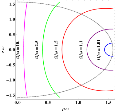
Figure 1: Structure of the SOL for various values of $\Omega/\omega$ in a $z$-$\rho$ plot, in units of $\omega^{-1}$, with the boundary of adS represented by the dotted curve. The interior of adS is contained within the dotted curve. The SOL only forms when $\Omega\geq\omega$. When $\Omega=\omega$ the SOL is situated on the equator of adS at the boundary (i.e. $r\omega=\theta=\pi/2$). As $\Omega$ increases, the SOL approaches the rotation axis and becomes more cylindrical in shape.

4.1 Rotating vacuum states

Geometrically, the metrics (2) and (27) describe the same space-time, using different coordinates. However, the natural choice of Hamiltonian, $H=i\partial_{t}$, differs in the two pictures. The Hamiltonian for the rotating observer $H_{\rm{rot}}$ contains a partial derivative with respect to $t$ holding $\varphi_{R}=\varphi-\Omega t$ constant whereas the Hamiltonian for a non-rotating observer $H_{\rm{adS}}$ contains a partial derivative with respect to $t$ holding $\varphi$ constant. Therefore, the two Hamiltonians are related by $H_{\rm rot}=H_{\rm adS}+i\Omega\partial_{\varphi}$.

Field modes $U_{\ell}$ have positive frequency if $HU_{\ell}=E_{\ell}U_{\ell}$ with $E_{\ell}>0$. Since they have different Hamiltonians, the rotating and non-rotating observers have different definitions of positive frequency. The adS modes $U_{\ell}$ have adS energy $E_{\ell}$, where $H_{\rm{adS}}U_{\ell}=E_{\ell}U_{\ell}$ and co-rotating modes ${\widetilde{U}}_{\ell}$ have co-rotating energy ${\widetilde{E}}_{\ell}$, where $H_{\rm{rot}}{\widetilde{U}}_{\ell}={\widetilde{E}}_{\ell}{\widetilde{U}}_{\ell}$. The co-rotating modes $\widetilde{U}_{\ell}$ can be obtained by performing a coordinate transformation on the adS modes $U_{\ell}$, namely: $\widetilde{U}_{\ell}(x)=e^{i\Omega tM_{z}}U_{\ell}(x)$, where $M_{z}$ is the $z$ component of the angular momentum operator. Choosing the modes $U_{\ell}$ to be simultaneous eigenvectors of $H_{\rm{adS}}$ and $M_{z}$ (on adS, $\mathinner{\left[{H_{\rm{adS}}},{M_{z}}\right]}=0$ art:cota ), the adS and co-rotating energies are related by ${\widetilde{E}}_{\ell}=E_{\ell}-\Omega m_{\ell}$, where $m_{\ell}$ is the $z$ component of the angular momentum of mode $\ell$. The non-rotating and rotating observers therefore define modes to have positive frequency if $E_{\ell}>0$ and ${\widetilde{E}}_{\ell}>0$ respectively.

Canonical quantization interprets modes with positive frequency as particle modes, while modes with negative frequency are interpreted as anti-particle modes. The general solution of the Dirac equation $\psi(x)$ is expanded in terms of field modes and promoted to an operator (here we consider the co-rotating modes):

$$\psi(x)=\sum_{\ell}\theta({\widetilde{E}}_{\ell})[\widetilde{U}_{\ell}(x)\widetilde{b}_{\ell}+\widetilde{V}_{\ell}(x)\widetilde{d}^{\dagger}_{\ell}],$$ (29)

where the anti-particle modes $\widetilde{V}_{\ell}$ are the charge conjugates of the particle modes (and therefore have negative frequency): $\widetilde{V}_{\ell}=i\gamma^{\hat{\,2}}\widetilde{U}_{\ell}^{*}$, and $\gamma^{\,\hat{2}}$ is the Minkowski $\gamma$ matrix. The one-particle operators satisfy the canonical anti-commutation relations: $\mathinner{\left\{{{\widetilde{b}}_{\ell}},{{\widetilde{b}}^{\dagger}_{\ell^{\prime}}}\right\}}=\mathinner{\left\{{{\widetilde{d}}_{\ell}},{{\widetilde{d}}^{\dagger}_{\ell^{\prime}}}\right\}}=\delta_{\ell\ell^{\prime}}$, $\mathinner{\left\{{{\widetilde{b}}_{\ell}},{{\widetilde{b}}_{\ell^{\prime}}}\right\}}=\mathinner{\left\{{{\widetilde{d}}_{\ell}},{{\widetilde{d}}_{\ell^{\prime}}}\right\}}=0$. The vacuum state corresponding to this choice of positive frequency is the state annihilated by all the one-particle annihilation operators ${\widetilde{b}}_{\ell}$, ${\widetilde{d}}_{\ell}$.

The non-rotating and rotating observers have different definitions of positive frequency and, accordingly, will define different vacuum states by the above procedure. The non-rotating adS vacuum is analogous to the global Minkowski vacuum, while the rotating vacuum corresponds to Iyer’s quantization art:iyer for rotating states in Minkowski space. Since thermal quantum states are defined relative to a vacuum state (see, for example, (22)), the different rotating and non-rotating vacua give rise to different t.e.v.s. A similar effect arises in Minkowski space, where defining rotating thermal states relative to the global Minkowski vacuum gives rise to t.e.v.s containing temperature-independent terms art:ambrusrot ; art:vilenkin which are not present if the rotating vacuum is used instead.

AdS has a time-like boundary which quantizes the non-rotating mode energies. As a result of this energy quantization, it can be shown art:cota ; art:ambrusads that $E_{\ell}\geq\omega m_{\ell}$. Hence, ${\widetilde{E}}_{\ell}\geq 0$ for all values of $\ell$ if $\Omega\leq\omega$ (i.e. when there is no SOL), in which case the rotating vacuum actually coincides with the adS vacuum. If $\Omega>\omega$, then the rotating and non-rotating vacua are distinct.

4.2 Rotating thermal states: $\Omega\leq\omega$

When $\Omega\leq\omega$, the rotating and non-rotating vacua coincide. Hence, the vacuum Feynman propagator $\widetilde{S}_{F}(x,x^{\prime})$ can be calculated from the non-rotating propagator $S_{F}(x,x^{\prime})$ by applying a coordinate transformation:

$$\widetilde{S}_{F}(x,x^{\prime})=e^{i\Omega tM_{z}}S_{F}(x,x^{\prime})e^{-i\Omega t^{\prime}M_{z}},$$ (30)

where $e^{-i\Omega t^{\prime}M_{z}}$ acts from the right on $S_{F}(x,x^{\prime})$. The thermal propagator can be constructed using the method outlined in Eq. (22). In addition to the t.e.v.s of the non-rotating case, there is a non-vanishing current of neutrinos (i.e. particles of negative helicity), which can be calculated using:

$$\braket{:J^{\hat{\alpha}}_{\nu}:}_{\beta}=-\lim_{x^{\prime}\rightarrow x}{\rm tr}\left[\gamma^{\hat{\alpha}}\frac{1-\gamma^{5}}{2}\Delta\widetilde{S}_{F}^{\beta}(x,x^{\prime})\right].$$ (31)

The resulting non-zero t.e.v.s have the following components with respect to the tetrad (28):

$$\braket{:\overline{\psi}\psi:}_{\beta}= -\frac{\omega^{3}\Gamma_{k}}{2\pi^{2}}\sum_{j=1}^{\infty}(-1)^{j}\cosh\frac{\omega j\beta}{2}\cosh\frac{\Omega j\beta}{2}\zeta_{j}^{2+k}{}_{2}F_{1}\left(1+k,2+k;1+2k;-\zeta_{j}\right),$$ (32a)

$$\braket{:J^{\hat{r}}_{\nu}:}_{\beta}= \frac{\omega^{3}\Gamma_{k}\cos\theta}{4\pi^{2}\cos\omega r}\sum_{j=1}^{\infty}(-1)^{j}\sinh\frac{\omega j\beta}{2}\sinh\frac{\Omega j\beta}{2}\zeta_{j}^{2+k}{}_{2}F_{1}\left(k,2+k;1+2k;-\zeta_{j}\right),$$ (32b)

$$\braket{:J^{\hat{\theta}}_{\nu}:}_{\beta}= -\frac{\omega^{3}\Gamma_{k}\sin\theta}{4\pi^{2}}\sum_{j=1}^{\infty}(-1)^{j}\sinh\frac{\omega j\beta}{2}\sinh\frac{\Omega j\beta}{2}\zeta_{j}^{2+k}{}_{2}F_{1}\left(k,2+k;1+2k;-\zeta_{j}\right),$$ (32c)

$$\braket{:T_{\hat{t}\hat{t}}:}_{\beta}= -\frac{\omega^{4}\Gamma_{k}}{4\pi^{2}\cos^{2}\omega r}\sum_{j=1}^{\infty}(-1)^{j}\cosh\frac{\omega j\beta}{2}\cosh\frac{\Omega j\beta}{2}$$

$$\times\left[2(2+k)\sinh^{2}\frac{\omega j\beta}{2}\zeta_{j}^{3+k}{}_{2}F_{1}\left(k,3+k;1+2k;-\zeta_{j}\right)-\cos^{2}\omega r\,\zeta_{j}^{2+k}{}_{2}F_{1}\left(k,2+k;1+2k;-\zeta_{j}\right)\right],$$ (32d)

$$\braket{:T_{\hat{t}\hat{\varphi}}:}_{\beta}= \frac{\omega^{4}\Gamma_{k}\sin\omega r\sin\theta}{8\pi^{2}\cos^{2}\omega r}\sum_{j=1}^{\infty}(-1)^{j}\sinh\frac{\omega j\beta}{2}\sinh\frac{\Omega j\beta}{2}$$

$$\times 2(2+k)\left(\cosh^{2}\frac{\omega j\beta}{2}+\cosh^{2}\frac{\Omega j\beta}{2}\right)\zeta_{j}^{3+k}{}_{2}F_{1}\left(k,3+k;1+2k;-\zeta_{j}\right),$$ (32e)

$$\braket{:T_{\hat{r}\hat{r}}:}_{\beta}= -\frac{\omega^{4}\Gamma_{k}}{4\pi^{2}}\sum_{j=1}^{\infty}(-1)^{j}\cosh\frac{\omega j\beta}{2}\cosh\frac{\Omega j\beta}{2}\zeta_{j}^{2+k}{}_{2}F_{1}\left(k,2+k;1+2k;-\zeta_{j}\right),$$ (32f)

$$\braket{:T_{\hat{\varphi}\hat{\varphi}}:}_{\beta}= -\frac{\omega^{4}\Gamma_{k}}{4\pi^{2}\cos^{2}\omega r}\sum_{j=1}^{\infty}(-1)^{j}\cosh\frac{\omega j\beta}{2}\cosh\frac{\Omega j\beta}{2}\left[\cos^{2}\omega r\,\zeta_{j}^{2+k}{}_{2}F_{1}\left(k,2+k;1+2k;-\zeta_{j}\right)\right.$$

$$\left.+2(2+k)\sinh^{2}\frac{\Omega j\beta}{2}\sin^{2}\omega r\sin^{2}\theta\,\zeta_{j}^{3+k}{}_{2}F_{1}\left(k,3+k;1+2k;-\zeta_{j}\right)\right],$$ (32g)

and $\braket{:T_{\hat{\theta}\hat{\theta}}:}_{\beta}=\braket{:T_{\hat{r}\hat{r}}:}_{\beta}$. In (32),

$$\zeta_{j}=\frac{\cos^{2}\omega r}{\sinh^{2}(\omega j\beta/2)-\sin^{2}\omega r\sin^{2}\theta\sinh^{2}(\Omega j\beta/2)},$$ (33)

and $\Gamma_{k}$ is given in Eq. (25). When $\Omega=0$, $\zeta_{j}$ reduces to $z_{j}$ defined in Eq. (25) and Eqs. (32) reduce to Eqs. (24). Equations (32) are regular for any combination of the parameters (i.e. $k$, $\beta$, $\Omega$, $\omega$, $r$ and $\theta$), as long as $\Omega<\omega$. Figure 2 shows $\braket{:T_{\hat{t}\hat{t}}:}_{\beta}$ at fixed $\beta$ for various values of $\Omega<\omega$, for both massless and massive fermions. It can be seen that the thermal state becomes more energetic as $\Omega$ increases.

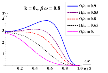
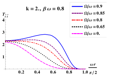
(a)	(b)

Figure 2: Thermal expectation values $\braket{:T_{\hat{t}\hat{t}}:}_{\beta}$ for fermions of mass $\mu=0$ (left) and $\mu=2\omega$ (right) in the equatorial plane ($\theta=\pi/2$) for $\beta\omega=0.8$ and $\Omega/\omega=0$ (non-rotating adS), $0.65$, $0.8$, $0.85$ and $0.9$. The thermal state becomes more energetic as $\Omega$ increases.

In the special case $\Omega=\omega$, the tetrad components $\braket{:T_{\hat{t}\hat{t}}:}$, $\braket{:T_{\hat{t}\hat{\varphi}}:}$ and $\braket{:T_{\hat{\varphi}\hat{\varphi}}:}$ diverge as the adS equator is approached (i.e. as $\theta\rightarrow\pi/2$ and $\omega r\rightarrow\pi/2$), due to the $\cos^{2}\omega r$ factor in the denominator inside the sum over $j$ (see Fig. 3). Equations (32) simplify considerably when $k=0$ and $\Omega=\omega$:

$$\braket{:\overline{\psi}\psi:}_{\beta}\rfloor_{\begin{subarray}{c}\Omega=\omega\\ k=0\end{subarray}}= -\frac{\omega^{3}(\cos\omega r)^{4}}{2\pi^{2}\varepsilon^{2}}\sum_{j=1}^{\infty}\frac{(-1)^{j}\cosh^{2}(\omega j\beta/2)}{\displaystyle\left(\cosh^{2}\frac{\omega j\beta}{2}-\frac{\sin^{2}\omega r\cos^{2}\theta}{\cos^{2}\omega r+\sin^{2}\omega r\sin^{2}\theta}\right)^{2}},$$ (34a)

$$\braket{:J^{\hat{r}}_{\nu}:}_{\beta}\rfloor_{\begin{subarray}{c}\Omega=\omega\\ k=0\end{subarray}}= -\frac{\omega^{3}(\cos\omega r)^{3}\cos\theta}{4\pi^{2}\varepsilon^{2}}S_{2}(\omega\beta),$$ (34b)

$$\braket{:J^{\hat{\theta}}_{\nu}:}_{\beta}\rfloor_{\begin{subarray}{c}\Omega=\omega\\ k=0\end{subarray}}= \frac{\omega^{3}(\cos\omega r)^{4}\sin\theta}{4\pi^{2}\varepsilon^{2}}S_{2}(\omega\beta),$$ (34c)

$$\braket{:T_{\hat{t}\hat{t}}:}_{\beta}\rfloor_{\begin{subarray}{c}\Omega=\omega\\ k=0\end{subarray}}= \frac{\omega^{4}(\cos\omega r)^{4}(4-\varepsilon)}{4\pi^{2}\varepsilon^{3}}[S_{4}(\omega\beta)+S_{2}(\omega\beta)],$$ (34d)

$$\braket{:T_{\hat{t}\hat{\varphi}}:}_{\beta}\rfloor_{\begin{subarray}{c}\Omega=\omega\\ k=0\end{subarray}}= -\frac{\omega^{4}(\cos\omega r)^{4}\sin\omega r\sin\theta}{\pi^{2}\varepsilon^{3}}[S_{4}(\omega\beta)+S_{2}(\omega\beta)],$$ (34e)

$$\braket{:T_{\hat{r}\hat{r}}:}_{\beta}\rfloor_{\begin{subarray}{c}\Omega=\omega\\ k=0\end{subarray}}= \frac{\omega^{4}(\cos\omega r)^{4}}{4\pi^{2}\varepsilon^{2}}[S_{4}(\omega\beta)+S_{2}(\omega\beta)],$$ (34f)

$$\braket{:T_{\hat{\varphi}\hat{\varphi}}:}_{\beta}\rfloor_{\begin{subarray}{c}\Omega=\omega\\ k=0\end{subarray}}= \frac{\omega^{4}(\cos\omega r)^{4}(4-3\varepsilon)}{4\pi^{2}\varepsilon^{3}}[S_{4}(\omega\beta)+S_{2}(\omega\beta)],$$ (34g)

where $S_{\ell}(x)=-\sum_{j=1}^{\infty}(-1)^{j}/[\sinh(jx/2)]^{\ell}$. The series $S_{2}(x)$ arising in the tetrad components of the neutrino charge current can be written using the Q-Pochhammer symbol $(a;q)_{k}=\prod_{n=0}^{k}(1-aq^{n})$ NIST :

$$S_{2}(x)=-4\frac{d}{dx}\ln(-1,e^{-x})_{\infty}.$$ (35)

It is remarkable that, apart from the fermion condensate, the coordinate dependance for all the t.e.v.s in Eqs. (34) is contained in trigonometric prefactors.

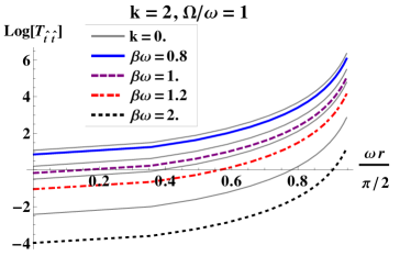
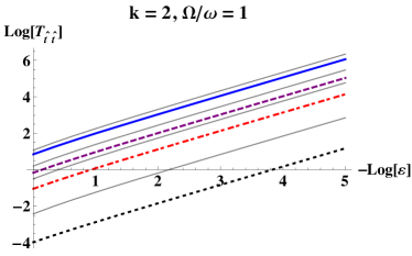
(a)	(b)

Figure 3: Comparison of thermal expectation values $\braket{:T_{\hat{t}\hat{t}}:}_{\beta}$ of massless (thin lines) and massive ($\mu=2\omega$) fermions in the equatorial plane ($\theta=\pi/2$) for $\Omega/\omega=1.0$ and $\beta\omega=0.8$, $1$, $1.2$ and $2$. Plot (a) shows $\ln\braket{:T_{\hat{t}\hat{t}}:}_{\beta}$ against the distance from the rotation axis, while plot (b) shows a logarithmic plot against $\ln\varepsilon^{-1}$, where $\varepsilon=1-\sin^{2}\omega r$. It can be seen that the divergence is of order $\varepsilon^{-1}$ irrespective of the value of the mass.

4.3 Rotating thermal states: $\Omega>\omega$

We have seen that some t.e.v.s diverge as the inverse distance to the adS equator when $\Omega=\omega$. If $\Omega$ is further increased, all t.e.v.s become divergent as inverse powers of the distance $\varepsilon$ to the SOL. Since the vacuum state changes if $\Omega>\omega$, the Feynman propagator method used up until now is no longer applicable. In this case, the t.e.v.s have to be calculated using mode sums art:ambrusrot .

Figure 4 shows the energy density as the SOL is approached, confirming that $\braket{:T_{\hat{t}\hat{t}}:}_{\beta}$ diverges as an inverse power of the distance to the SOL. While further analytic investigations are required to confirm the exact order of this divergence, numerical results show that its order is higher than in the case $\Omega=\omega$. The leading order divergence seems to be the same regardless of the mass of the fermions.

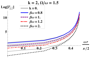
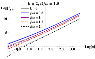
(a)	(b)

Figure 4: Comparison of thermal expectation values $\braket{:T_{\hat{t}\hat{t}}:}_{\beta}$ of massless (thin lines) and massive ($\mu=2\omega$) fermions in the equatorial plane ($\theta=\pi/2$) for $\Omega/\omega=1.5$ and $\beta\omega=0.8$, $1$, $1.2$ and $2$. Plot (a) shows $\ln\braket{:T_{\hat{t}\hat{t}}:}_{\beta}$ against the distance from the rotation axis, while plot (b) shows a logarithmic plot against $\ln\varepsilon^{-1}$.

5 Conclusions

In this paper, we considered quantum states of fermions of arbitrary mass in anti-de Sitter space (adS) as seen by an observer rotating with a constant angular velocity $\Omega$. In the non-rotating case ($\Omega=0$), the geometric properties of adS were used to construct the Feynman propagator in closed form, from which vacuum expectation values for the fermion condensate (FC) and stress-energy tensor (SET) were calculated using Hadamard renormalization. Thermal expectation values were calculated using a closed form expression for the bi-spinor of parallel transport.

In the case when $0<\Omega\leq\omega$, we found that the rotating and non-rotating vacua were the same. Thus, the non-rotating vacuum Feynman propagator was used to derive expressions for the thermal expectation values (t.e.v.s) of the FC, neutrino charge current (CC) and SET. If $\Omega<\omega$, all t.e.v.s stay finite throughout adS. When $\Omega>\omega$, mode sums were required to evaluate t.e.v.s. For these values of $\Omega$ a speed of light surface (SOL) forms and t.e.v.s diverge as inverse powers of the distance to this SOL. If $\Omega=\omega$, the SOL collapses down to a curve on the equator of adS. In this case, the FC, CC, $T_{\hat{r}\hat{r}}$ and $T_{\hat{\theta}\hat{\theta}}$ stay constant throughout the equatorial plane while $T_{\hat{t}\hat{t}}$, $T_{\hat{t}\hat{\varphi}}$ and $T_{\hat{\varphi}\hat{\varphi}}$ diverge as $1/\cos^{2}\omega r$ as $\omega r\rightarrow\pi/2$.

References

- (1) O. Aharony, S. S. Gubser, J. M. Maldacena, H. Ooguri, and Y. Oz, Phys. Rept. 323, 183–386 (2000).
- (2) W. Mück, J. Phys. A 33, 3021–3026 (2000).
-
(3)
V. E. Ambru
and E. Winstanley, Proceedings of the first Karl-Schwarzschild Meeting KSM2013, arXiv:1310.7429 [gr-qc] (2013).s , - (4) A.-H. Najmi and A. C. Ottewill, Phys. Rev. D 30, 2573–2578 (1984).
- (5) C. Dappiaggi, T.-P. Hack, and N. Pinamonti, Rev. Math. Phys. 21, 1241–1312 (2009).
-
(6)
V. E. Ambru
and E. Winstanley, preprint arXiv:1401.6388 [hep-th] (2014).s , -
(7)
V. E. Ambru
and E. Winstanley, Proceedings of the thirteenth Marcel Grossman meeting MG13, arXiv:1302.3791 [gr-qc] (2013).s , -
(8)
V. E. Ambru
and E. Winstanley, Rotating fermions on adS, paper in preparation.s , - (9) I. Cotăescu, Rom. J. Phys. 52, 895–940 (2007).
- (10) B. Allen and T. Jacobson, Commun. Math. Phys. 103, 669–692 (1986).
-
(11)
V. E. Ambru
and E. Winstanley, Fermions on adS, paper in preparation.s , - (12) Y. Decanini and A. Folacci, Phys. Rev. D 78, 044025 (2008).
- (13) P. B. Groves, P. R. Anderson, and E. D. Carlson, Phys. Rev. D 66, 124017 (2002).
- (14) R. Camporesi and A. Higuchi, Phys. Rev. D 45, 3591–3603 (1992).
- (15) B. R. Iyer, Phys. Rev. D 26, 1900–1905 (1982).
- (16) A. Vilenkin, Phys. Rev. D 21, 2260–2269 (1980).
- (17) F. W. J. Olver, D. W. Lozier, R. F. Boisvert, and C. W. Clark, NIST Handbook of Mathematical Functions, (Cambridge University Press, Cambridge, 2010), p. 436.