Variational Image Segmentation Model Coupled with Image Restoration Achievements

Abstract

Image segmentation and image restoration are two important topics in image processing with great achievements. In this paper, we propose a new multiphase segmentation model by combining image restoration and image segmentation models. Utilizing image restoration aspects, the proposed segmentation model can effectively and robustly tackle high noisy images, blurry images, images with missing pixels, and vector-valued images. In particular, one of the most important segmentation models, the piecewise constant Mumford-Shah model, can be extended easily in this way to segment gray and vector-valued images corrupted for example by noise, blur or missing pixels after coupling a new data fidelity term which comes from image restoration topics. It can be solved efficiently using the alternating minimization algorithm, and we prove the convergence of this algorithm with three variables under mild condition. Experiments on many synthetic and real-world images demonstrate that our method gives better segmentation results in comparison to others state-of-the-art segmentation models especially for blurry images and images with missing pixels values.

1 Introduction

Image segmentation and image restoration are two important subjects in image processing. Image segmentation consists in partitioning a given image into multiple segments to transfer the representation of the image into a more meaningful one which is easier to analyze. It is typically used to locate objects and boundaries within an image. Image restoration is the operation of estimating the desired clean image from its corrupted version. Corruption may come in many forms, such as blur, noise, camera misfocus, or information lost. Obviously, image segmentation can be used as preprocessing or postprocessing of image restoration. In other words, these two topics can influence each other.

Let $\Omega\subset\mathbb{R}^{2}$ be a bounded, open, connected set, and $f:\Omega\rightarrow\mathbb{R}$ a given image. Without loss of generality, we restrict the range of $f$ to [0,1]. Let $g:\Omega\rightarrow\mathbb{R}$ denote the desired clean image, then $f=g+n_{f}$, when $n_{f}$ is the additive noise. Many image restoration models can be written in the form

$$E(g)=\lambda\Phi(f,g)+\phi(g),$$ (1)

where $\Phi(f,g)$ is the data fidelity term, $\phi(g)$ is the regularization term, and $\lambda>0$ is a regularization parameter balancing the trade-off between terms $\Phi(f,g)$ and $\phi(g)$. If set $\Phi(f,g)=\int_{\Omega}(f-g)^{2}dx$ and $\phi(g)=\int_{\Omega}|\nabla g|dx$ (total variation term), then model (1) goes to the ROF model proposed by Rudin, Osher and Fatemi in 1992 [35], i.e.,

$$E(g)=\lambda\int_{\Omega}(f-g)^{2}dx+\int_{\Omega}|\nabla g|dx.$$ (2)

One important advantage of model (2) is that it preserves the edge information of $f$ very well, but also introduces the staircase effect. To remove the staircase effect, many works are designed based on higher-order derivative terms, see [5, 14, 28, 36, 42]. For example in [5], the tight-frame technic was used in $\phi(g)$ to obtain more details of the higher-order derivative information from $f$. The relationship between the total variation and the tight-frame can be found in [39]. As we know, the data fidelity term $\Phi(f,g)=\int_{\Omega}(f-g)^{2}dx$ is especially effective for Gaussian noise [35]. For removing other types of noise than Gaussian noise, $\Phi(f,g)=\int_{\Omega}(g-f\log g)dx$ and $\Phi(f,g)=\int_{\Omega}|f-g|dx$ are proposed for Poisson noise and impulsive noise in [17] and [30], respectively. Please refer to [1, 11, 12, 17, 24, 30, 26, 37, 38] and references therein for the details of the Poisson noise and impulsive noise removal. Note that the image restoration model (1) can be extended to process blurry image after introducing a problem related linear operator ${\cal A}$ in front of $g$ [34].

Let $\Gamma\in\Omega$ represent the boundary of the objects within an image, and $\Omega_{i}$ be the parts of the segmented objects fulfill $\Omega=\cup_{i}\Omega_{i}\cup\Gamma$. The Mumford-Shah model is one of the most important image segmentation models, and has been studied extensively in the last twenty years. More precisely, in [29], Mumford and Shah proposed an energy minimization problem which approximates the true solution by finding optimal piecewise smooth approximations. The energy minimization problem was formulated as

$$E(g,\Gamma)=\frac{\lambda}{2}\int_{\Omega}(f-g)^{2}dx+\frac{\mu}{2}\int_{\Omega\setminus\Gamma}|\nabla g|^{2}dx+{\rm Length}(\Gamma),$$ (3)

where $\lambda$ and $\mu$ are positive parameters, and $g:\Omega\rightarrow\mathbb{R}$ is continuous or even differentiable in $\Omega\setminus\Gamma$ but may be discontinuous across $\Gamma$. Because model (3) is nonconvex, it is very challenging to find or approximate its minimizer, see [8, 9, 21]. Many works [25, 41] concentrate on simplifying model (3) by restricting $g$ to be piecewise constant function ($g=c_{i}$ in $\Omega_{i}$), i.e.,

$$E(g,\Gamma)=\frac{\lambda}{2}\sum_{i=1}^{K}\int_{\Omega_{i}}(f-c_{i})^{2}dx+{\rm Length}(\Gamma),$$ (4)

where $K$ is the number of phases. Using the coarea formula [20], model (4) can be rewritten as

$$\begin{split}E(c_{i},u_{i})&=\lambda\sum_{i=1}^{K}\int_{\Omega}(f-c_{i})^{2}u_{i}dx+\sum_{i=1}^{K}\int_{\Omega}|\nabla u_{i}|dx,\\ {\rm s.t.}&\quad\sum_{i=1}^{K}u_{i}(x)=1,u_{i}(x)\in\{0,1\},\forall x\in\Omega.\end{split}$$ (5)

Moreover, model (5) with $K=2$ is the Chan-Vese model [16], and with fixed $c_{i}$ is a special case of the Potts model [33]. Due to the nonconvex property of (5), in [13], the exact convex version of (5) was proposed when $K=2$ and $c_{i}$ fixed. For $K>2$, recently, several authors are focused on relaxing $u_{i}$ and solving the following model

$$\begin{split}E(u_{i},c_{i})&=\lambda\sum_{i=1}^{K}\int_{\Omega}(f-c_{i})^{2}u_{i}dx+\sum_{i=1}^{K}\int_{\Omega}|\nabla u_{i}|dx,\\ {\rm s.t.}&\quad\sum_{i=1}^{K}u_{i}(x)=1,u_{i}(x)\geq 0,\forall x\in\Omega.\end{split}$$ (6)

Please refer to [2, 23, 27, 32, 43] and references therein for more details related with (6). One drawback of model (6) is that it can not segment images corrupted by blur or information lost, which is one main problem to solve in this paper.

In [31], a model of coupling image restoration and segmentation based on a statistical framework of generalized linear models was proposed, but the analysis and algorithm therein are only focused on two-phase segmentation problem. In our previous work [6], a two-stage segmentation method which provides a better understanding of the link between image segmentation and image restoration was proposed. The method suggests that for segmentation, it is reasonable and practicable to extract the different phases in $f$ from using image restoration methods first and thresholding followed. Moreover, in our recent work [7], we proved that the solution of the Chan-Vese model [16] for certain $\lambda$ can actually be given by thresholding the minimizer of the ROF model (2) using a proper threshold, which clearly provides one kind of relationships between image segmentation and image restoration.

In this paper, start from extending the piecewise constant Mumford-Shah model (4) to manage blurry image, a novel segmentation model by composing model (4) with a data fidelity term which comes from image restoration topics is proposed. Since only a new fidelity term is added, and usually the fidelity term possesses good property such as differentiable, the solution of the proposed model is not more involved comparing with solving model (4). It can be solved efficiently using the alternating minimization (AM) algorithm [18] with the ADMM or primal-dual algorithms [4, 10, 22]. We prove that under mild condition, the AM algorithm converges for the proposed model. The proposed model can segment blurry images easily but model (4) can not. Moreover, it can also deal with images with information lost and vector-valued images for example color images. Due to the advantage of two data fidelity terms, one from image restoration and the other from image segmentation, our model is much more robust and stable. Experiments on many kinds of synthetic and real-world images demonstrate that our method gives better segmentation results in comparison with other state-of-the-art segmentation methods especially for blurry images and images with missing pixels values.

Contributions. The main contributions of this paper are summarized as follows.

• Coupling the variational image segmentation models and the image restoration models, which provides a new way for multiphase image segmentation.

• Extend the piecewise constant Mumford-Shah model (4) by cooperating the image restoration achievements so that the new constructed variation segmentation model can handle blurry case easily.

• Thanks to the image restoration achievements, the new variation segmentation model has the potential to process many different types of noises, for example Gaussian, Poisson, and impulsive noises.

• The kinds of vector-valued image for example the color image and the observed image with information lost are also covered in the proposed variational segmentation model.

• The convergence of the AM algorithm with three variables to the proposed variational model is proved.

The rest of this paper is organized as follows. In Section 2, we propose our new segmentation model and extend it so that it can deal with vector-valued images and images with some pixels values missing. In Section 3, the AM algorithm to our model will be introduced. The convergence of it will be proved in Section 4. In Section 5, the comparison of the proposed method on various synthetic and real-world images with the state-of-the-art multiphase segmentation methods will be shown. Conclusions are given in Section 6.

2 The Proposed Variational Image Segmentation Model

We propose our image segmentation model by combining the piecewise constant Mumford-Shah model (5) with the fidelity term $\Phi(f,g)$ which comes from the image restoration model (1). More precisely, our proposed segmentation model aims to minimize the energy

$$\begin{split}E(u_{i},c_{i},g)&=\mu\Phi(f,{\cal A}g)+\lambda\Psi(g,u_{i},c_{i})+\sum_{i=1}^{K}\int_{\Omega}|\nabla u_{i}|dx,\\ {\rm s.t.}&\quad\sum_{i=1}^{K}u_{i}(x)=1,u_{i}(x)\in\{0,1\},\forall x\in\Omega,\end{split}$$ (7)

where $g\in L^{2}(\Omega)$ and ${\cal A}$ is the problem related linear operator. For example ${\cal A}$ can be the identity operator for a noisy observed image $f$ or a blurring operator if there are noise and blur in $f$. The first term $\Phi(f,{\cal A}g)$ is the data fidelity term arising from the image restoration model (1). It controls $g$ not far away from the given corrupted image $f$, in other words, it aims to deblure and denoise according to the types of noises in $f$. Term $\Psi(g,u_{i},c_{i})$ is also the data fidelity term but comes from the image segmentation model, which aims to separate $g$ into $K$ specified segments. In this paper, we restrict ourselves to

$$\Psi(u_{i},c_{i},g)=\sum_{i=1}^{K}\int_{\Omega}(g-c_{i})^{2}u_{i}dx.$$

The last term in (7) is the regularization term which controls the length of the boundaries of the segmented parts $u_{i}$. The type of the used data fidelity term $\Phi(f,{\cal A}g)$ changes according to different noise models, for example,

• Gaussian noise: $\Phi(f,{\cal A}g)=\int_{\Omega}(f-{\cal A}g)^{2}dx$;

• Poisson noise (I-divergence): $\Phi(f,{\cal A}g)=\int_{\Omega}\big{(}{\cal A}g-f\log({\cal A}g)\big{)}dx$;

• Impulsive noise: $\Phi(f,{\cal A}g)=\int_{\Omega}|f-{\cal A}g|dx$.

Compared with model (5), the model (7), in addition to the ability of segmenting blurry images, its two data fidelity terms make it much more robust and stable to process the observed corrupted image $f$.

Obviously, for fixed $g$, model (7) is reduced to model (5). The following theorem 1 gives the uniqueness of $g$ when minimizingl (7) for fixed $c_{i}$ and $u_{i}$.

Theorem 1.

Assume $\Phi(f,{\cal A}g)$ in (7) is convex and continuous, then there exists one and only one $g$ which minimizes energy (7) for fixed $c_{i}$ and $u_{i}$.

Proof.

See the Appendix. ∎

In the following, we restrict ourselves to $\Phi(f,{\cal A}g)=\int_{\Omega}(f-{\cal A}g)^{2}dx$ as one example to show how to extend model (7) so that it can handle images with missing information and vector-valued images. Let $\Omega^{\prime}$ be the set containing the pixels whose pixels values are missing. Then model (7) can be extended to segment images with missing information as

$$E(u_{i},c_{i},g)=\mu\int_{\Omega}(f-{\cal A}g)^{2}\omega dx+\lambda\sum_{i=1}^{K}\int_{\Omega}(g-c_{i})^{2}\omega u_{i}dx+\sum_{i=1}^{K}\int_{\Omega}|\nabla u_{i}|dx,$$ (8)

where

$$\sum_{i=1}^{K}u_{i}(x)=1,u_{i}(x)\in\{0,1\},\ \omega(x)=\begin{cases}1,\quad{\rm if}\ x\in\Omega\setminus\Omega^{\prime},\\ 0,\quad{\rm otherwise}.\end{cases}$$ (9)

For the observed vector-valued image represented as $\boldsymbol{f}=(f_{1},\cdots,f_{N})$, let $\boldsymbol{g}=(g_{1},\cdots,g_{N})$ and ${\boldsymbol{c}}_{i}=(c_{i,1},\cdots,c_{i,N})$, model (7) can be extended to segment vector-valued images with missing pixels values as

$$E(u_{i},{\boldsymbol{c}}_{i},\boldsymbol{g})=\mu\sum_{j=1}^{N}\int_{\Omega}(f_{j}-{\cal A}_{j}g_{j})^{2}\omega dx+\lambda\sum_{i=1}^{K}\sum_{j=1}^{N}\int_{\Omega}(g_{j}-c_{i,j})^{2}\omega u_{i}dx+\sum_{i=1}^{K}\int_{\Omega}|\nabla u_{i}|dx,$$ (10)

where $u_{i}$ and $\omega$ are defined in (9).

3 The AM Algorithm

We first transfer (7) by relaxing $u_{i}$ to the following version

$$E(u_{i},c_{i},g){}={} \mu\Phi(f,{\cal A}g)+\lambda\sum_{i=1}^{K}\int_{\Omega}(g-c_{i})^{2}\omega u_{i}dx+\sum_{i=1}^{K}\int_{\Omega}|\nabla u_{i}|dx,$$ (11)

$${\rm s.t.}\quad \sum_{i=1}^{K}u_{i}(x)=1,u_{i}(x)\geq 0,\forall x\in\Omega.$$ (12)

Using the AM algorithm, a partial minimizer $(g,c_{i},u_{i})$ of (11) can be computed alternatively as follows:

• Find $g$ as minimizer of (11) for fixed $u_{i}$ and $c_{i}$. Obviously, $g$ is only contained in the first two terms of (11), and the second term can be regarded as one kind of Tikhonov regularizations when solving $g$, see [40]. The algorithm to find $g$ depends on the choice of $\Phi(f,{\cal A}g)$. For example when $\Phi(f,{\cal A}g)=\int_{\Omega}(f-{\cal A}g)^{2}\omega dx$, since it is differentiable, we have

  $$g=(\mu{\cal A}^{T}{\cal A}+\lambda)^{-1}\big{(}\mu{\cal A}^{T}f+\lambda\sum_{i=1}^{K}c_{i}u_{i}\big{)}\omega.$$ (13)

  For solving $g$ according to the choice of $\Phi(f,{\cal A}g)$ to Poisson noise or impulsive noise, we leave this problem in our future work.

• Find $c_{i}$ as minimizer of (11) for fixed $u_{i}$ and $g$. Let $c=(c_{1},\cdots,c_{K})$, clearly, $c_{i}$ is just related with the second term of (11), therefore

  $$c_{i}=\frac{\int_{\Omega}g\omega u_{i}dx}{\int_{\Omega}\omega u_{i}dx}.$$ (14)

• Find $u_{i}$ as minimizer of (11) for fixed $g$ and $c_{i}$. The discussion of this is given in the following.

Note that when $g$ is fixed, the first term of model (11) is constant, hence the problem of finding $u_{i}$ is reduced to minimize model (6) with $\omega$. Therefore, there are many methods we can use, for example the ADMM method in [4, 22, 23] which will be given explicitly in the following. Alternatively, one can apply the primal-dual algorithm [10, 32] or the max-flow approach [43].

Let $u(j)=(u_{i}(j))_{i=1}^{K},s=(s_{i})_{i=1}^{K}=\big{(}(g-c_{i})^{2}\omega\big{)}_{i=1}^{K}$, then our problem can be transferred to be

$$\min_{v,u,d}\lambda\langle v,s\rangle+\|d\|_{1}+\iota_{S}(u),\quad{\rm s.t.}\quad\nabla v=d,v=u,$$ (15)

where $\iota_{S}(\cdot)$ is the indicator function defined as

$$\iota_{S}(y):=\begin{cases}0,&{\rm if}\ y\in S,\\ +\infty,&{\rm otherwise},\end{cases}$$

and $S:=\{y\in\mathbb{R}^{K}|\sum_{i=1}^{K}y_{i}=1,y\geq 0\}$. Then iterate the following steps until converge

$$\begin{split}v^{k+1}{}={}&\mathop{\rm argmin}_{v}\Big{\{}\lambda\langle v,s\rangle+\sigma(\|b_{d}^{k}+\nabla v-d^{k}\|^{2}+\|b_{u}^{k}+v-u^{k}\|^{2})\Big{\}},\\ d^{k+1}{}={}&\mathop{\rm argmin}_{d}\Big{\{}\|d\|_{1}+\sigma\|b_{d}^{k}+\nabla v^{k+1}-d\|^{2}\Big{\}},\\ u^{k+1}{}={}&\mathop{\rm argmin}_{d}\Big{\{}\iota_{S}(u)+\sigma\|b_{u}^{k}+v^{k+1}-u\|^{2}\Big{\}},\\ b_{d}^{k+1}{}={}&b_{d}^{k}+\nabla v^{k+1}-d^{k+1},\\ b_{u}^{k+1}{}={}&b_{u}^{k}+v^{k+1}-u^{k+1}.\end{split}$$ (16)

After $u=(u_{i})_{i=1}^{K}$ is solved, each segment $\Omega_{i}$ can be obtained by

$$\Omega_{i}=\Big{\{}x|u_{i}(x)=\max\big{\{}u_{1}(x),\cdots,u_{K}(x)\big{\}},\forall x\in\Omega\Big{\}}.$$ (17)

In summary, the AM algorithm to solve model (11) is given in Algorithm 1.

Algorithm 1 The AM Algorithm to Model (11)

0:  Observed image $f$, number of phases $K$, $c^{(0)}$, and $u^{(0)}$.

1:  while $\|c^{(k+1)}-c^{k}\|>\epsilon$ do

2:        find $g^{(k+1)}$ as minimizer of (11) for fixed $u^{(k)}$, and $c^{(k)}$ using (13);

3:        find $c^{(k+1)}$ as minimizer of (11) for fixed $g^{(k+1)}$ and $u^{(k)}$ using (14);

4:        find $u^{(k+1)}$ as minimizer of (11) for fixed $g^{(k+1)}$ and $c^{(k+1)}$ using (16);

5:  end while

6:  return  $\Omega_{i},i=1,\ldots,K$ using (17) 

4 Convergence Analysis

In this section, we discuss the convergence property of Algorithm 1. We first give the very general conclusion to the AM algorithm for three variables. Let $X\subset\mathbb{R}^{m_{1}},Y\subset\mathbb{R}^{m_{2}}$ and $Z\subset\mathbb{R}^{m_{3}}$ be closed sets, and the energy function $E:X\times Y\times Z\rightarrow\mathbb{R}$ be continuous and bounded from below. To process the AM algorithm, we start with some initial guess $y^{(0)},z^{(0)}$, then one successively obtains the alternating sequence (between $z,y$ and $x$) of conditional minimizers

$$z^{(0)},y^{(0)}\rightarrow x^{(0)}\rightarrow z^{(1)}\rightarrow y^{(1)}\rightarrow x^{(1)}\rightarrow\cdots$$

from solving, for $k=0,1,\ldots$,

$$\begin{split}x^{(k)}&\in\mathop{\rm argmin}_{x}E(x,y^{(k)},z^{(k)}),\\ z^{(k+1)}&\in\mathop{\rm argmin}_{z}E(x^{(k)},y^{(k)},z),\\ y^{(k+1)}&\in\mathop{\rm argmin}_{y}E(x^{(k)},y,z^{(k+1)}).\end{split}$$ (18)

Theorem 2.

(Monotonicity of Alternating Minimization). Let $X\subset\mathbb{R}^{m_{1}},Y\subset\mathbb{R}^{m_{2}}$ and $Z\subset\mathbb{R}^{m_{3}}$ be closed sets, and $E:X\times Y\times Z\rightarrow\mathbb{R}$ be continuous and bounded from below. Then, for each $k\geq 0$, the following relations are satisfied

$$E(x^{(k)},y^{(k+1)},z^{(k+1)}) \leq E(x^{(k-1)},y^{(k)},z^{(k)}),$$

$$E(x^{(k)},y^{(k)},z^{(k+1)}) \leq E(x^{(k-1)},y^{(k-1)},z^{(k)}),$$

$$E(x^{(k+1)},y^{(k+1)},z^{(k+1)}) \leq E(x^{(k)},y^{(k)},z^{(k)}).$$

Hence, the sequence $\big{\{}E(x^{(k)},y^{(k)},z^{(k)})_{k\in\mathbb{N}}\big{\}}$ converges monotonically.

Proof.

See the Appendix. ∎

Theorem 3.

Let $X\subset\mathbb{R}^{m_{1}},Y\subset\mathbb{R}^{m_{2}}$ and $Z\subset\mathbb{R}^{m_{3}}$ be closed sets, and $E:X\times Y\times Z\rightarrow\mathbb{R}$ be continuous and bounded from below. Then, for any convergent subsequence $(x^{(k_{i})},y^{(k_{i})},z^{(k_{i})})_{i\in\mathbb{N}}$ of $(x^{(k)},y^{(k)},z^{(k)})_{k\in\mathbb{N}}$ generated from formula (18) with

$$(x^{(k_{i})},y^{(k_{i})},z^{(k_{i})})\longrightarrow(x^{*},y^{*},z^{*}),\ {\rm as}\ i\rightarrow\infty,$$

the following relations are satisfied:

$$\begin{split}E(x^{*},y^{*},z^{*})\leq E(x,y^{*},z^{*})&\quad\forall x\in X,\\ E(x^{*},y^{*},z^{*})\leq E(x^{*},y,z^{*})&\quad\forall y\in Y,\\ E(x^{*},y^{*},z^{*})\leq E(x^{*},y^{*},z)&\quad\forall z\in Z.\end{split}$$ (19)

$(x^{*},y^{*},z^{*})$ is called the the partial minimizer of $E(\cdot,\cdot,\cdot)$ if (19) is satisfied.

Proof.

See the Appendix ∎

Let $\cal O$ be the set of all the partial minimizers of model (11) defined in Theorem 3. The following theorem 4 gives the convergence property of Algorithm 1.

Theorem 4.

Assume the operator $\cal A$ in model (11) is a continuous mapping and $\Phi(f,{\cal A}g)$ is continuous and nonnegative. As $k\rightarrow\infty$, if $(u^{(k)},g^{(k)},c^{(k)})\rightarrow(u^{*},g^{*},c^{*})$, then $(u^{*},g^{*},c^{*})\in{\cal O}$. If $(u^{(k)},g^{(k)},c^{(k)})_{k\in\mathbb{N}}$ does not converge, it must contain a convergent subsequence and every convergent subsequence converges to a partial minimizer of model (11).

Proof.

See the Appendix. ∎

5 Experimental Results

We compare our segmentation model (11) with three state-of-the-art multiphase segmentation methods [6, 23, 43] for different phases synthetic and real-world images corrupted by noise, blur and missing pixels. More precisely, methods [43] and [23] minimize model (6) by using the max-flow approach and the ADMM algorithm, respectively. The difference between methods [43] and [23] is that method [43] minimizes $u_{i}$ with fixed $c_{i}$, while method [23] minimizes $u_{i}$ and $c_{i}$ both. Method [6] is a two-stage segmentation method, which solves a convex variant of the Mumford-Shah model (3) first and a thresholding technique followed. Moreover, method [6] is very effective in segmenting general kind of images including blurry images. All the codes of methods [6, 23, 43] are provided by the authors, and the parameters in them are chosen by trial and error to give the best results of the respective methods. Note that all the methods [6, 23, 43] can only segment gray images. In order to compare the effectiveness of our model (11) with model (6) in color images, we first extend model (6) using the strategy in (10) so that it can handle color images, then method [23] will be adopted to solve the extended model (6). That means the comparison in color images will be executed between our method and the extended method [23].

The initial codebook $c_{i}$ for methods [23, 43] are computed by the fuzzy C-means method [3] with 100 iteration steps, and the thresholds chosen in the thresholding technique of method [6] is using the automatic strategy therein. The tolerance $\epsilon$ and the step size $\sigma$ respectively in Algorithm 1 and (16) are fixed to be $10^{-4}$ and $2$. The parameters $\lambda$ and $\mu$ in model (11) are chosen empirically.

For adding Gaussian noise to the given image $f\in[0,1]$, we apply the MATLAB command imnoise with zero mean and different variances for different kinds of images. In particular, the variance used to add noise into the blurry images is fixed to be $10^{-4}$. If there is no special explanation, to blur an image, the Gaussian kernel used is size $15\times 15$ with standard deviation 15 and the motion kernel is 15 pixels with an angle of 90 degrees. We apply the MATLAB command rand to remove some information from the corrupted images randomly, and set the percentage of information lost to be $40\%$ unless special explanation. The segmentation accuracy (SA) defined as

$$\textrm{SA}=\frac{\#\textrm{correctly classified pixels}}{\#\textrm{all pixels}}\times 100,$$

which will be used to evaluate the accuracy of the involved methods in detail. All the results were tested on a MacBook with 2.4 GHz processor and 4GB RAM.

(A1)	(B1) [43] (99.50)	(C1) [23] (99.64)	(D1) [6] (99.48)	(E1) Our (99.65)
(A2)	(B2) [43] (64.23)	(C2) [23] (98.13)	(D2) [6] (97.15)	(E2) Our (99.29)
(A3)	(B3) [43] (97.91)	(C3) [23] (98.37)	(D3) [6] (98.08)	(E3) Our (98.43)
(A4)	(B4) [43] (68.27)	(C4) [23] (74.28)	(D4) [6] (86.11)	(E4) Our (95.66)

Figure 1: Segmentation of two-phase synthetic images ($128\times 128$ and $195\times 195$). (A1) and (A3): the given noisy images; (A2) and (A4): the given noisy images with $40\%$ information lost; Columns two to five: the results of methods [43, 23, 6] and our method, respectively. Numbers in braces are the segmentation accuracy.

5.1 Gray image segmentation

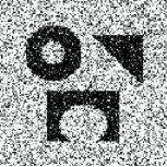
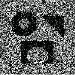
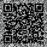
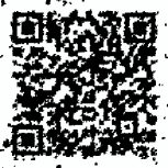
Example 1: two-phase synthetic images. To illustrate the ability of our method in high level noisy images and images with information lost, we first test it in two two-phase synthetic images, i.e. one contains different shapes, and the other is the 2D barcode image which represents data relating to the object it is attached and is the most frequently used type to scan with smartphones, see Fig. 1. Fig. 1(A1)–(A4) give the images corrupted by Gaussian noise with variance 0.2, and Fig. 1(A2) and (A4) give the images with part information removed randomly. The columns two to four of Fig. 1 are the results of methods [43, 23, 6], respectively. The last column of Fig. 1 is the results of our method. From the rows one and three of Fig. 1, the results of segmenting the given noisy images, we see that all the methods can give very good results. However, after comparing the segmentation accuracy given in the braces under each result, we get that our method gives the highest SA compared with others three methods. That means our model (11) can really improve the segmentation accuracy compared with model (6). From the second and the fourth rows of Fig. 1, the results of segmenting the given images with part information lost, we can easily see that only our method gives good results both in visual and segmentation accuracy.

(A1)	(B1) [43] (99.64)	(C1) [23] (99.63)	(D1) [6] (97.96)	(E1) Our (99.65)
(A2)	(B2) [43] (75.41)	(C2) [23] (86.89)	(D2) [6] (95.88)	(E2) Our (99.48)
(A3)	(B3) [43] (97.58)	(C3) [23] (98.63)	(D3) [6] (97.83)	(E3) Our (98.72)
(A4)	(B4) [43] (85.61)	(C4) [23] (84.17)	(D4) [6] (86.11)	(E4) Our (97.45)

Figure 2: Segmentation of fourphase and fivephase synthetic images ($256\times 256$ and $91\times 91$). (A1) and (A3): the given noisy images; (A2) and (A4): the given noisy images with $20\%$ information lost; Columns two to five: the results of methods [43, 23, 6] and our method, respectively. Numbers in braces are the segmentation accuracy.

(A1)	(B1) [43] (86.05)	(C1) [23] (86.31)	(D1) [6] (95.61)	(E1) Our (99.44)
(A2)	(B2) [43] (90.42)	(C2) [23] (90.44)	(D2) [6] (97.24)	(E2) Our (99.92)
(A3)	(B3) [43] (72.91)	(C3) [23] (72.66)	(D3) [6] (92.66)	(E3) Our (96.38)
(A4)	(B4) [43] (71.05)	(C4) [23] (71.25)	(D4) [6] (92.53)	(E4) Our (96.96)

Figure 3: Segmentation of fourphase and fivephase synthetic blurry images ($256\times 256$ and $91\times 91$). (A1) and (A3): the given images with Gaussion blur; (A2) and (A4): the given images with motion blur; Columns two to five: the results of methods [43, 23, 6] and our method, respectively. Numbers in braces are the segmentation accuracy.

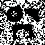
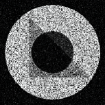
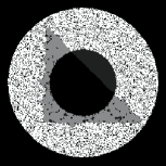
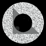
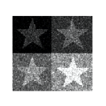
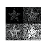
Example 2: multiphase synthetic images. Two multiphase synthetic images will be tested in this example, i.e., one is four phases image with different shapes inside, and the other is five phases image including stars with different intensities. In Fig. 2(A1)–(A4), the variances used to add noise on the four phases and five phases images are 0.05 and 0.01, respectively. Moreover, Fig. 2(A2) and (A4) give the noisy images with $20\%$ of all pixels randomly removed. From the results in Fig. 2, we can get very similar conclusions as those obtained in example 1, i.e., all the methods give very good results for noisy images but our method gives the highest segmentation accuracy which illustrates our model (11) is superior compared with model (6); and only our method can give good results when the given images with information lost.

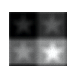
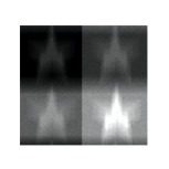
To illustrate the effect of our method in segmenting blurry images, we first test our method in two synthetic multiphase images used in Fig. 2 but with Gaussion blur and motion blur involved, see Fig. 3. Fig. 3(A3) is blurred by using the gaussian kernel with size $10\times 10$ and standard deviation 10. After comparing with our method with methods [43, 23, 6] in Fig. 3, we see that only method [6] and our method can give good results. More precisely, after comparing the segmentation accuracy of method [6] and our method, we can see that our method gives much higher SA which means our method gives better results than method [6]. Methods [43, 23] are not able to segment the blurry images correctly. More precisely, for the results of methods [43, 23] in Fig. 3(A1) and (A2), the pixels around the boundaries are segmented uncorrectly; for their results in Fig. 3(A3) and (A4), even one star located in the right bottom corner is missed for both methods [43] and [23].

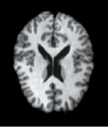
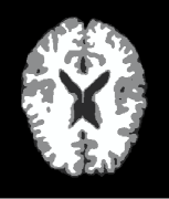
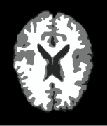
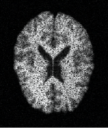
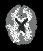
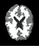
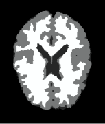
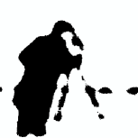
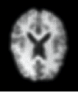
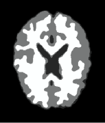
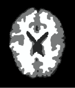
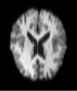
Example 3: real-world images. Test our method in two real-world images, i.e., camera man and MRI (magnetic resonance imaging) brain image which comes from medical imaging subject, see Fig. 4. We first test our method in noisy images and images with information lost. In Fig. 4, the variance used for adding noise is 0.01, and the percentage of information lost is $20\%$. The conclusions we get are very close to those obtained when we test the methods in synthetic images in examples 1 and 2. From the rows one and three of Fig. 4, we see that all the methods give very good results in segmenting the two original real-world images. But for the images with information lost especially for the image in Fig. 4(A4), the results of methods [43, 23] are worse than the results of methods [6] and ours, see Fig. 4(B4), (C4), (D4), and (E4). Moreover, for the results of methods [6] and ours, we see that our result gives much more details for the white matter, see Fig. 4(D4) and (E4).

The ability of our method in segmenting blurry images is given in Fig. 5. After comparing the results in Fig. 5, we can see that method [6] and our method give very similar good results, on the contrary, the results of methods [43, 23] are worse.

(A1)	(B1) [43]	(C1) [23]	(D1) [6]	(E1) Our
(A2)	(B2) [43]	(C2) [23]	(D2) [6]	(E2) Our
(A3)	(B3) [43]	(C3) [23]	(D3) [6]	(E3) Our
(A4)	(B4) [43]	(C4) [23]	(D4) [6]	(E4) Our

Figure 4: Segmentation of real-world images: camera man and MRI brain ($256\times 256$ and $319\times 256$). (A1) and (A3): the given images; (A2) and (A4): the given noisy images with $20\%$ information lost; Columns two to five: the results of methods [43, 23, 6] and our method, respectively.

(A1)	(B1) [43]	(C1) [23]	(D1) [6]	(E1) Our
(A2)	(B2) [43]	(C2) [23]	(D2) [6]	(E2) Our
(A3)	(B3) [43]	(C3) [23]	(D3) [6]	(E3) Our
(A4)	(B4) [43]	(C4) [23]	(D4) [6]	(E4) Our

Figure 5: Segmentation of real-world blurry images: camera man and MRI brain ($256\times 256$ and $319\times 256$). (A1) and (A3): the given images with Gaussion blur; (A2) and (A4): the given images with motion blur; Columns two to five: the results of methods [43, 23, 6] and our method, respectively.

5.2 Color image segmentation

Example 4: two-phase rose image. Fig. 6(A1)–(A4) give the original rose image, and the original image corrupted by part information removed randomly, Gaussian blur and motion blur, respectively. The columns two and three in Fig. 6 give the results of the extended method [23] and our method, respectively. After the comparison, we see that both of the two methods can give good results for the original image, see the first row of Fig. 6; from the second row of Fig. 6, we see that the boundary of the result of the extended method [23] is coarse compared with our result; from rows three and four of Fig. 6, we can see that the boundaries of the results of the extended method [23] are over smoothed compared with our results. Hence, we have that our model can get better results in segmenting blurry color images, while the extended method [23] can not. Moreover, from the results of our method, we can see that the results of our method for the corrupted images are as good as the result of our method for the original image, see the third column of Fig. 6. This really demonstrates the ability of our method in segmenting images with information lost or blur.

(A1)	(A2)	(A3)	(A4)
(B1) Extended [23]	(B2) Extended [23]	(B3) Extended [23]	(B4) Extended [23]
(C1) Our	(C2) Our	(C3) Our	(C4) Our

Figure 6: Segmentation of rose color image ($303\times 250\times 3$). Row one: the given image, and the given images corrupted by $40\%$ information lost, Gaussian blur, and motion blur, respectively. Rows two to three: the results of the extended method [23] and our method, respectively.

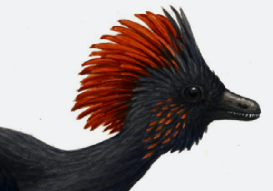
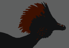
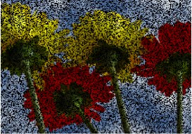
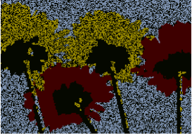
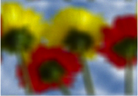
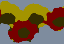
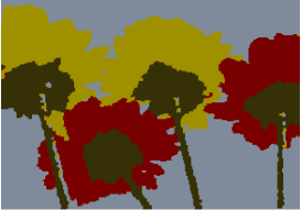
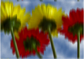
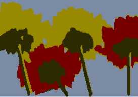
Example 5: multiphase images. Finally, in order to demonstrate the ability of our method in segmenting color images with information lost and blur much more clearly, we test our method in two more multiphase color images, i.e. three phases crown image and four phases flowers image, see Fig. 7 and Fig. 8, respectively. Fig. 7(A1) (Fig. 8(A1)) is the original crown (flowers) image, and Fig. 7(A2)–(A4) (Fig. 8(A2)–(A4)) are the images corrupted by part information removed randomly, Gaussian blur and motion blur, respectively. Obviously, the extended method [23] fails for segmenting the images with information lost, see Fig. 7(B2) and Fig. 8(B2). Moreover, from Fig. 7(C2) and (D2) and Fig. 8(C2) and (D2), we can see that the extended method [23] gives over smoothed results for blurry color images. On the contrary, from the third column of Fig. 7 and Fig. 8, the results of our method, we see that all the results of our method are very good. Moreover, the results of our method for the corrupted images are as good as the results of our method for the original crown and flowers images.

(A1)	(B1) Extended [23]	(C1) Our
(A2)	(B2) Extended [23]	(C2) Our
(A3)	(B3) Extended [23]	(C3) Our
(A4)	(B4) Extended [23]	(C4) Our

Figure 7: Segmentation of crown color image ($225\times 300\times 3$). Column one: the given image, and the given images corrupted by $40\%$ information lost, Gaussian blur, and motion blur, respectively. Columns two to three: the results of the extended method [23] and our method, respectively.

(A1)	(B1) Extended [23]	(C1) Our
(A2)	(B2) Extended [23]	(C2) Our
(A3)	(B3) Extended [23]	(C3) Our
(A4)	(B4) Extended [23]	(C4) Our

Figure 8: Segmentation of flowers color image ($188\times 250\times 3$). Column one: the given image, and the given images corrupted by $40\%$ information lost, Gaussian blur, and motion blur, respectively. Columns two to three: the results of the extended method [23] and our method, respectively.

6 Conclusions

In this paper, we proposed a new multiphase segmentation model by combining the image restoration approaches with the variational image segmentation model. Utilizing image restoration aspects, the proposed segmentation model is very effective and robust to tackle noisy images, blurry images, and images with missing pixels. In particular, the piecewise constant Mumford-Shah model was extended using our strategy so that it can process blurry images. Moreover, our model can also be extended to process vector-valued images for example the color images. It can be solved efficiently using the AM algorithm, and we prove its convergence property under mild condition. Experiments on many kinds of synthetic and real-world images demonstrate that our method gives better segmentation results in comparison with others state-of-the-art segmentation methods especially in blurry images and images with missing pixels values. In our future work, we will test our model in images corrupted by other types of noise, for example the Poisson noise and the impulsive noise, etc.

Acknowledgement: The main part of this work has been done in the University of Kaiserslautern, Germany. Thanks to Prof. Gabriele Steidl (University of Kaiserslautern) for fruitful discussions and invaluable comments.

Appendix

Proof of Theorem 1

Proof.

Fix $c_{i}=c_{i}^{*}$ and $u_{i}=u_{i}^{*}$. Note that $L^{2}(\Omega)$ is a reflective Banach space, and $E(g,c_{i}^{*},u_{i}^{*})$ in (7) is convex and lower semicontinuous. Using Proposition 1.2 in [19], for the existence of $g$, we just need to prove that $E(g,c_{i}^{*},u_{i}^{*})$ is coercive over $L^{2}(\Omega)$. The coercive of $E(g,c_{i}^{*},u_{i}^{*})$ can be given by

$$\|g\|_{2} = \|\sum_{i=1}^{K}(g-c_{i})u_{i}+\sum_{i=1}^{K}c_{i}u_{i}\|_{2}$$

$$\leq \|\sum_{i=1}^{K}|g-c_{i}|u_{i}^{\frac{1}{2}}\|_{2}+\|\sum_{i=1}^{K}c_{i}u_{i}\|_{2}$$

$$\leq \sqrt{K}\sqrt{\sum_{i=1}^{K}\int_{\Omega}(g-c_{i})^{2}u_{i}dx}+\|\sum_{i=1}^{K}c_{i}u_{i}\|_{2}$$

$$\leq \frac{\sqrt{K}}{\sqrt{\lambda}}\sqrt{E(g,c_{i}^{*},u_{i}^{*})}+\|\sum_{i=1}^{K}c_{i}u_{i}\|_{2}.$$

Moreover, since the middle term of energy (7) is quadratic with respect to $g$, hence energy (7) is strictly convex, therefore it has unique minimizer $g$ for fixed $c_{i}$ and $u_{i}$. ∎

Proof of Theorem 2

Proof.

From (18), it can be verified easily that

$$E(x^{(k+1)},y^{(k+1)},z^{(k+1)}) \leq E(x^{(k)},y^{(k+1)},z^{(k+1)})$$

$$\leq E(x^{(k)},y^{(k)},z^{(k+1)})$$

$$\leq E(x^{(k)},y^{(k)},z^{(k)})$$

$$\leq E(x^{(k-1)},y^{(k)},z^{(k)})$$

$$\leq E(x^{(k-1)},y^{(k-1)},z^{(k)}).$$

Hence, since $E(\cdot,\cdot,\cdot)$ is bounded from below, the sequence $\big{\{}E(x^{(k)},y^{(k)},z^{(k)})\big{\}}_{k\in\mathbb{N}}$ converges monotonically. ∎

6.1 Proof of Theorem 3

Proof.

Using (18) and the idea of [15, Theorem 5.5], for each $i$

$$E(x^{(k_{i})},y^{(k_{i})},z^{(k_{i})})\leq E(x,y^{(k_{i})},z^{(k_{i})})\quad\forall x\in X.$$

By the continuity of $E(\cdot,\cdot,\cdot)$, this gives, as $i\rightarrow\infty$,

$$E(x^{*},y^{*},z^{*})\leq E(x,y^{*},z^{*})\quad\forall x\in X.$$

On the other hand, for each $i$, note that $k_{i-1}\leq k_{i}-1$. From Theorem 2, we have for $\forall y\in Y$,

$$E(x^{(k_{i})},y^{(k_{i})},z^{(k_{i})}) \leq E(x^{(k_{i}-1)},y^{(k_{i})},z^{(k_{i})})$$

$$\leq E(x^{(k_{i-1})},y^{(k_{i-1}+1)},z^{(k_{i-1}+1)})$$

$$\leq E(x^{(k_{i-1})},y,z^{(k_{i-1}+1)}),$$

and $\forall z\in Z$,

$$E(x^{(k_{i})},y^{(k_{i})},z^{(k_{i})}) \leq E(x^{(k_{i}-1)},y^{(k_{i})},z^{(k_{i})})$$

$$\leq E(x^{(k_{i}-1)},y^{(k_{i}-1)},z^{(k_{i})})$$

$$\leq E(x^{(k_{i-1})},y^{(k_{i-1})},z^{(k_{i-1}+1)})$$

$$\leq E(x^{(k_{i-1})},y^{(k_{i-1})},z).$$

Coupled with the continuity of $E(\cdot,\cdot,\cdot)$, as $i\rightarrow\infty$, we have,

$$E(x^{*},y^{*},z^{*})\leq E(x^{*},y,z^{*})\quad{\rm and}\quad E(x^{*},y^{*},z^{*})\leq E(x^{*},y^{*},z)$$

for $\forall y\in Y$ and $\forall z\in Z$ respectively. ∎

Proof of Theorem 4

Proof.

For model (11), because all of its three terms are continuous and nonnegative, we have $E(\cdot,\cdot,\cdot)$ is continuous and nonnegative. If $(u^{(k)},g^{(k)},c^{(k)})\rightarrow(u^{*},g^{*},c^{*})$, as $k\rightarrow\infty$, using Theorem 3, we have $(u^{*},g^{*},c^{*})\in{\cal O}$. Obviously, the whole components of $u^{(k)}$ are in $[0,1]$, hence $u^{(k)}$ is bounded. From (14), we get $c^{(k)}$ is bounded since it is just the convex combination of $g$. From (13), we have

$$\|g\|_{2} \leq \|(\mu{\cal A}^{T}{\cal A}+\lambda{\cal I})^{-1}\|_{2}\|\big{(}\mu{\cal A}^{T}f+\lambda\sum_{i=1}^{K}c_{i}u_{i}\big{)}\omega\|_{2}$$

$$\leq \big{(}\mu\|{\cal A}^{T}\|_{2}\|f\|_{2}+\lambda\sum_{i=1}^{K}c_{i}\|u_{i}\|_{2}\big{)}\|\omega\|_{2}/\lambda,$$

hence $g^{(k)}$ is also bounded. Therefore $(u^{(k)},g^{(k)},c^{(k)})_{k\in\mathbb{N}}$ must contain convergent subsequence. Using Theorem 3, we can get that any of these subsequences converges to a partial minimizer of model (11). ∎

References

- [1] G. Aubert and J. Aujol, “A variational approach to removing multiplicative noise,” SIAM J. Appl. Math., vol. 68, no. 4, pp. 925–946, Jan. 2008.
- [2] L. Bar, T. Chan, G. Chung, M. Jung, N. Kiryati, R. Mohieddine, N. Sochen, and L.A. Vese, “Mumford and Shah model and its applications to image segmentation and image restoration,” Handbook of Mathematical Imaging, Springer, pp. 1095–1157, 2011.
- [3] J. Bezdek, R. Ehrlich, and W. Full, “FCM: The fuzzy -means clustering algorithm,” Comput. Geosci., vol. 10, no. 2-3, pp. 191–203, 1984.
- [4] S. Boyd, N. Parikh, E. Chu, B. Peleato, and J. Eckstein, “Distributed optimization and statistical learning via the alternating direction method of multipliers,” Found. and Trends Mach. Learning, vol. 3, no. 1, pp. 1–122, Jan. 2010.
- [5] J. Cai, R. H. Chan, and Z. Shen, “A framelet-based image inpainting algorithm,” Appl. Comput. Harmon. A., vol. 24, no. 2, pp. 131–149, Mar. 2008.
- [6] X. Cai, R. Chan, and T. Zeng, “A two-stage image segmentation method using a convex variant of the Mumford-Shah model and thresholding,” SIAM J. Imaging Sci., vol. 6, no. 1, pp. 368–390, Feb. 2013.
- [7] X. Cai and G. Steidl, “Multiclass segmentation by iterated ROF thresholding,” EMMCVPR, LNCS, Springer, pp. 237–250, 2013.
- [8] A. Chambolle, “Image segmentation by variational methods: Mumford and Shah functional and the discrete approximations,” SIAM J. Appl. Math., vol. 55, no. 3, pp. 827–863, 1995.
- [9] A. Chambolle, “Finite differences discretization of the Mumford-Shah functional,” RAIRO Math. Model. Numer. Anal., vol. 33, no. 2, pp. 261–288, 1999.
- [10] A. Chambolle and T. Pock, “A first-order primal-dual algorithm for convex problems with applications to imaging,” J. math. Imaging Vis., vol. 40, no. 1, pp. 120–145, May 2011.
- [11] R. Chan, C. Hu, and M. Nikolova, “An iterative procedure for removing random-valued impulse noise,” IEEE Signal Process. Lett., vol. 11, no. 12, pp. 921–924, Dec. 2004.
- [12] R. Chan, C. Hu, and M. Nikolova, “Salt-and-pepper noise removal by median-type noise detectors and detail-preserving regularization,” IEEE Trans. Image Process., vol. 14, no. 10, pp. 1479–1485, Oct. 2005.
- [13] T. Chan, S. Esedoglu, and M. Nikolova, “Algorithms for finding global minimizers of image segmentation and denoising models,” SIAM J. Appl. Math, vol. 66, no. 5, pp. 1632–1648, Sep. 2006.
- [14] T. Chan, A. Marquina, and P. Mulet, “High-order total variation-based image restoration,” SIAM J. Sci. Comput., vol. 22, no. 2, pp. 503–516, 2000.
- [15] T. Chan and J. Shen, “Image processing and analysis: variational, PDE, wavelet, and stochastic methods,” SIAM, 2005.
- [16] T. Chan and L.A. Vese, “Active contours without edges,” IEEE Trans. Image Process., vol. 10, no. 2, pp. 266–277, Feb. 2001.
- [17] I. Csiszár, “Why least squares and maximum entropy? An axiomatic approach to inference for linear inverse problems,” The Annals of Statistics, vol. 19, no. 4, pp. 2032–2066, 1991.
- [18] I. Csiszár and G. Tusnady, “Information geometry and alternating minimization procedures,” Statistics Decisions, Supplement Issu, vol. 1, pp. 205–237, 1984.
- [19] I. Ekeland and R. Temam, “Convex analysis and variational problems,” SIAM, Philadelphia, 1999.
- [20] W. Fleming, W. Rishel, and R. Rishel, “An integral formula for total gradient variation,” Arch. Math., vol. 11, no. 1, pp. 218–222, 1960.
- [21] M. Gobbino, “Finite difference approximation of the Mumford-Shah functional,” Comm. Pure Appl. Math., vol. 51, no. 2, pp. 197–228, Feb. 1998.
- [22] T. Goldstein and S. Osher, “The split Bregman algorithm for L1 regularized problems,” SIAM J. Imaging Sci., vol. 2, no. 2, pp. 323–343, Apr. 2009.
- [23] Y. He, B. Shafei, M. Y. Hussaini, J. Ma, and G. Steidl, “A new fuzzy c-means method with total variation regularization for segmentation of images with noisy and incomplete data,” Pattern Recognition, vol. 45, no. 9, pp. 3436-3471, Sep. 2012.
- [24] Y. Huang, M. Ng, and Y. Wen, “Fast image restoration methods for impulse and Gaussian noise removal,” IEEE Signal Process. Lett., vol. 16, no. 6, pp. 457–460, Jun. 2009.
- [25] G. Koepfler, C. Lopez, and J. Morel, “A Multiscale Algorithm for Image Segmentation by Variational Approach,” SIAM J. Numer. Anal., vol. 31, no. 1, pp. 282–299, Feb. 1994.
- [26] T. Le, R. Chartrand and T. Asaki, “A variational approach to reconstructing images corrupted by Poisson noise,” J. Math. Imaging Vis., vol. 27, no. 3, pp. 257–263, Apr. 2007.
- [27] F. Li, M. Ng, T. Zeng, and C. Shen, “A multiphase image segmentation method based on fuzzy region competition,” SIAM J. Imaging Sci., vol. 3, no. 3, pp. 277–299, Jul. 2010.
- [28] M. Lysaker, A. Lundervold, and X. Tai, “Noise removal using fourth-order partial differential equation with applications to medical magnetic resonance images in space and time,” IEEE Trans. on Image Process., vol. 12, no. 12, pp. 1579–1590, Dec. 2003.
- [29] D. Mumford and J. Shah, “Optimal approximations by piecewise smooth functions and associated variational problems,” Comm. Pure Appl. Math., vol. 42, no. 5, pp. 577–685, Jul. 1989.
- [30] M. Nikolova, “A variational approach to remove outliers and impulse noise,” J. Math. Imag. Vis., vol. 20, no. 1-2, pp. 99–120, Jan. 2004.
- [31] G. Paul, J. Cardinale, and I. Sbalzarini, “Coupling image restoration and segmentation: a generalized linear model/bregman perspective,” Int. J. Comput. Vis., vol. 104, no. 1, pp. 69–93, Aug. 2013.
- [32] T. Pock, D. Cremers, A. Chambolle, and H. Bischof, “A convex relaxation approach for computing minimal partitions,” Proceedings of the IEEE Computer Society Conference on Computer Vision and Pattern Recognition (CVPR), pp. 810–817, 2009.
- [33] R. Potts, “Some generalized order-disorder transformations,” Proceedings of the Cambridge Philosophical Society 48, pp. 106–109, 1952.
- [34] L. Rudin and S. Osher, “Total variation based image restoration with free local constraints,” Proc. 1st IEEE ICIP, vol. 1, pp. 31–35, 1994.
- [35] L. Rudin, S. Osher, and E. Fatemi, “Nonlinear total variation based noise removal algorithms,” Physica D., vol. 60, no. 1-4, pp. 259–268, Nov. 1992.
- [36] S. Setzer and G. Steidl, “Variational methods with higher order derivatives in image processing,” Approximation XII, Nashboro Press, Brentwood, pp.360–386, 2008.
- [37] S. Setzer, G. Steidl, and T. Teuber, “Deblurring Poissonian images by split Bregman techniques,” J. Vis. Commun. Image R., vol. 21, no. 3, pp. 193–199, Apr. 2010.
- [38] G. Steidl and T. Teuber, “Removing multiplicative noise by Douglas-Rachford splitting methods,” J. Math. Imaging and Vis., vol. 36, no. 2, pp. 168–184, Feb. 2010.
- [39] G. Steidl, J. Weickert, T. Brox, P. Mrazek, and M. Welk, “On the equivalence of soft wavelet shrinkage, total variation diffusion, total variation regularization, and SIDEs,” SIAM J. Numer. Anal., vol. 42, no. 2, pp. 686–713, May 2004.
- [40] A. Tikhonov, “Regularization of ill-posed problems,” Dokl. Akad. Nauk SSSR 153, vol. 1, pp. 49–52, 1963.
- [41] L. Vese and T. Chan, “A multiphase level set framework for image segmentation using the Mumford and Shah model,” Int. J. of Computer Vision, vol. 50, no. 3, pp. 271–293, Dec. 2002.
- [42] Y. You and M. Kaveh, “Fourth-order partial differential equation for noise removal,” IEEE Trans. on Image Process., vol. 9, no. 10, pp. 1723–1730, Oct. 2000.
- [43] J. Yuan, E. Bae, X. Tai, and Y. Boycov, “A continuous max-flow approach to potts model,” ECCV, 2010.