Optimization on the Hierarchical Tucker manifold - applications to tensor completion

Abstract.

In this work, we develop an optimization framework for problems whose solutions are well-approximated by Hierarchical Tucker (HT) tensors, an efficient structured tensor format based on recursive subspace factorizations. By exploiting the smooth manifold structure of these tensors, we construct standard optimization algorithms such as Steepest Descent and Conjugate Gradient for completing tensors from missing entries. Our algorithmic framework is fast and scalable to large problem sizes as we do not require SVDs on the ambient tensor space, as required by other methods. Moreover, we exploit the structure of the Gramian matrices associated with the HT format to regularize our problem, reducing overfitting for high subsampling ratios. We also find that the organization of the tensor can have a major impact on completion from realistic seismic acquisition geometries. These samplings are far from idealized randomized samplings that are usually considered in the literature but are realizable in practical scenarios. Using these algorithms, we successfully interpolate large-scale seismic data sets and demonstrate the competitive computational scaling of our algorithms as the problem sizes grow.

1. Introduction

The matrix completion problem is concerned with interpolating a $m\times n$ matrix from a subset of its entries. The amount of recent successes in developing solution techniques to this problem is a result of assuming a low-rank model on the 2-D signal of interest and by considering subsampling schemes that increase the rank of the underlying matrix [8], [7], [9]. The original signal is recovered by promoting low-rank structures subject to data constraints.

Using a similar approach, we consider the problem of interpolating a $d-$dimensional tensor from samples of its entries. That is, we aim to solve,

(1) $$\min_{\mathbf{X}\in\operatorname*{\mathcal{H}}}\frac{1}{2}\|P_{\Omega}\mathbf{X}-b\|^{2}_{2},$$

where $P_{\Omega}$ is a linear operator $P_{\Omega}:\mathbb{R}^{n_{1}\times n_{2}\times...\times n_{d}}\to\mathbb{R}^{m}$, $b\in\mathbb{R}^{m}$ is our subsampled data satisfying $b=P_{\Omega}\mathbf{X}^{*}$ for some “solution” tensor $\mathbf{X}^{*}$ and $\operatorname*{\mathcal{H}}$ is a specific class of low-rank tensors to be specified later. Under the assumption that $\mathbf{X}^{*}$ is well approximated by an element in $\operatorname*{\mathcal{H}}$, our goal is to recover $\mathbf{X}^{*}$ by solving (1). For concreteness, we concern ourselves with the case when $P_{\Omega}$ is a restriction operator, i.e.,

$$P_{\Omega}\mathbf{X}=\mathbf{X}_{i_{1},i_{2},\dots,i_{d}}\quad\text{ if }(i_{1},i_{2},\dots,i_{d})\in\Omega,$$

and $\Omega\subset[n_{1}]\times[n_{2}]\times\dots\times[n_{d}]$ is the so-called sampling set, where $[n]=\{1,\dots,n\}$. In the above equation, we suppose that $|\Omega|=m\ll n_{1}n_{2}\dots n_{d}$, so that $P_{\Omega}$ is a subsampling operator.

Unlike the matrix case, there is no unique notion of rank for tensors, as we shall see in Section 1.1, and there are multiple tensor formats that generalize a particular notion of separability from the matrix case—i.e, there is no unique extension of the SVD to tensors. Although each tensor format can lead to compressible representations of their respective class of low-rank signals, the truncation of a general signal to one of these formats requires access to the fully sampled tensor $\mathbf{X}$ (or at the very least query-based access to the tensor [4]) in order to achieve reasonable accuracy, owing to the use of truncated SVDs acting on various matricizations of the tensor. As in matrix completion, randomized missing entries change the behavior of the singular values and vectors of these matricizations and hence of the final approximation. Moreover, when the tensor of interest is actually a discretized continuous signal, there can be a number of constraints, physical or otherwise, that limit our ability to ideally sample it. For instance, in the seismic case, the tensor of interest is a multi-dimensional wavefield in the earth’s subsurface sampled at an array of receivers located at the surface. In real-world seismic experiments, budgetary constraints or environmental obstructions can limit both the total amount of time available for data acquisition as well as the number and placement of active sources and receivers. Since seismic and other methods rely on having fully sampled data for drawing accurate inferences, tensor completion is an important technique for a variety of scientific fields that acquire multidimensional data.

In this work, we consider the class of Hierarchical Tucker (abbreviated HT) tensors, introduced in [21, 18], as our low-rank tensors of interest. The set of all such tensors is a smooth, embedded submanifold of $\mathbb{R}^{n_{1}\times n_{2}\times...\times n_{d}}$, first studied in [42], which we equip with a Riemannian metric. Using this Riemannian structure, we can construct optimization algorithms in order to solve (1) for $d$-dimensional tensors. We will also study some of the effects of higher dimensional sampling and extend ideas from compressive sensing and matrix completion to the HT tensor case for our specific seismic examples.

1.1. Previous Work

To provide the reader with some context on tensor representations, let us briefly detail some of the available structured tensor formats, including tensor completion results, here (see [26] and [28] for a very comprehensive overview). Here we let $N=\max_{i=1\cdots d}n_{i}$ be the maximum individual dimension size, $N^{d}:=\prod_{i=1}^{d}n_{i}$ denote the dimension of the ambient space $\mathbb{R}^{n_{1}\times n_{2}\times...\times n_{d}}$, and, for each tensor format discussed, $K$ is the maximum of all of the rank parameters associated to that format.

The so-called Candecomp/Parafac (CP) decomposition is a very straightforward application of the separation of variables technique. Very much like the SVD of a matrix, one stipulates that, for a function $f$ living on a tensor product space, one can write

$$f(x_{1},x_{2},\dots,x_{d})\approx\sum_{i=1}^{K}f_{i}^{(1)}(x_{1})f_{i}^{(2)}(x_{2})\dots f_{i}^{(d)}(x_{d}).$$

Thus its discretization can be written as

$$\mathbf{f}\approx\sum_{i=1}^{K}f_{i}^{(1)}\otimes f_{i}^{(2)}\otimes\dots\otimes f_{i}^{(d)}$$

where $\otimes$ is the Kronecker product and $f_{i}^{(j)}\in\mathbb{R}^{n_{j}}$ is the discretization of the one dimensional function $f_{i}^{(j)}(x_{j})$. In addition to its intuitive construction, the CP decomposition of rank $K$ only requires $dNK$ parameters versus the $N^{d}$ of the full tensor and tensor-tensor operations can be performed efficiently on the underlying factors rather than the full tensors themselves (see [3] for a comprehensive set of MATLAB tools).

Unfortunately, despite the parsimoniousness of the CP construction, the approximation of an arbitrary (full) tensor by CP tensors has both theoretical and numerical difficulties. In particular, the set of all CP tensors of rank at most $K$ is not closed, and thus the notion of a best $K-$rank approximation is difficult to compute in many cases [13]. Despite this shortcoming, various authors have proposed iterative and non-iterative algorithms in the CP format for approximating full tensors [28] as well as interpolating tensors with missing data, such as the Alternating Least Squares approach (a block Gauss-Seidel type method) proposed alongside the CP format in [10] and [22], with convergence analysis in [41], and a nonlinear least-squares optimization scheme in [2].

The CP format is a specific case of the more general Tucker format, which aims to write a tensor $\mathbf{f}$ as a multilinear product

$$\mathbf{f}\approx U_{1}\times_{1}U_{2}\times_{2}\dots U_{d}\times_{d}\mathbf{C}$$

where $\mathbf{C}\in\mathbb{R}^{k_{1}\times k_{2}\times...\times k_{d}}$ is the so-called core tensor and the matrices $U_{j}\in\mathbb{R}^{n_{j}\times k_{j}}$, $j=1,\dots,d$ are the factors of the decomposition. Here we use the notation of the multilinear product, that is, $U_{i}\times_{i}\mathbf{C}$ indicates that $\mathbf{C}$ is multiplied by $U_{i}$ in dimension $i$, e.g., see [13, 28]. We will elaborate on this construction in Section 2.2. The CP format follows from this formulation when the core tensor is diagonal, i.e., $\mathbf{C}_{i_{1},i_{2},i_{3},\dots,i_{d}}=\mathbf{C}_{i_{1},i_{1},\dots,i_{1}}\delta_{i_{1},i_{2},\dots,i_{d}}$, where $\delta_{i_{1},i_{2},\dots,i_{d}}=1$ when $i_{1}=i_{2}=\dots=i_{d}$ and $0$ otherwise.

The Tucker format enjoys many benefits in terms of approximation properties over its CP counterpart. Namely, the set of all Tucker tensors of at most multilinear rank $\mathbf{k}=(k_{1},k_{2},\dots,k_{d})$ is closed and as a result every tensor $\mathbf{f}$ has a best at most multilinear rank-$\mathbf{k}$ Tucker approximation. A near-optimal approximation can be computed efficiently by means of the Higher Order SVD [12]. For the tensor completion problem, the authors in [17] consider the problem of recovering a Tucker tensor with missing entries using the Douglas-Rachford splitting technique, which decouples interpolation and regularization by nuclear norm penalization of different matricizations of the tensor into subproblems that are then solved via a particular proximal mapping. An application of this approach to seismic data is detailed in [29] for the interpolation problem and [30] for denoising. Depending on the size and ranks of the tensor to be recovered, there are theoretical and numerical indications that this approach is no better than penalizing the nuclear norm in a single matricization (see [36] for a theoretical justification in the Gaussian measurement case, as well as [39] for an experimental demonstration of this effect). Some preliminary results on theoretical guarantees for recovering low-rank Tucker tensors from subsampled measurements are given in [25] for pointwise measurements and a suitable, tensor-based incoherence condition and [35], which considers a nuclear norm penalty of the matricization of the first $d/2$ modes of $\mathbf{X}$ as opposed to a sum of nuclear norms of each of its $d$ modes, as is typically considered.

Aside from convex relaxations of the tensor rank minimization problem, the authors in [32] develop an alternative manifold-based approach to Tucker Tensor optimization similar to our considerations for the Hierarchical Tucker case and subsequently complete such tensors with missing entries. Each evaluation of the objective and Riemannian gradient requires $O(d(N+|\Omega|)K^{d}+dK^{d+1})$ operations, whereas our method only requires $O(dNK^{2}+d|\Omega|K^{3}+dK^{4})$ operations. As a result of using the Hierarchical Tucker format instead of the Tucker format, our method scales much better as $d$, $N$, and $K$ grow.

Previous work in completing tensors in the Tensor Train format, which is the Hierarchical Tucker format with a specific, degenerate binary dimension tree, includes [19, 23], wherein the authors use an alternating least-squares approach for the tensor completion problem. The derivations of the smooth manifold structure of the set of TT tensors can be found in [24]. This work is a precursor for the manifold structure of Hierarchical Tucker tensors studied in [42], upon which we expand in this article. For a comprehensive review of various tensor formats, we refer the reader to [27, 20].

Owing to its extremely efficient storage requirements (which are linear in the dimension $d$ as opposed to exponential in $d$), the Hierarchical Tucker format has enjoyed a recent surge in popularity for parametrizing high-dimensional problems. The hTucker toolbox [31] contains a suite of MATLAB tools for working with tensors in the HT format, including efficient vector space operations, matrix-tensor and tensor-tensor products, and truncations of full arrays to HT format. This truncation, the so-called Hierarchical SVD developed in [18], allows one to approximate a full tensor in HT format with a near-optimal approximation error. Even though the authors in [4] develop a HT truncation method that does not need access to every entry of the tensor in order to form the HT approximation, their approach requires algorithm-driven access to the entries, which does not apply for the seismic examples we consider below. A HT approach for solving dynamical systems is outlined in [33], which considers similar manifold structure as in this article applied in a different context.

1.2. Contributions and Organization

In this paper, we extend the primarily theoretical results of [42] to practical algorithms for solving optimization algorithms on the HT manifold. In Section 3.1, we introduce the Hierarchical Tucker format. We restate some of the results of [42] in Section 3.1 to provide context for the Riemannian metric we introduce on the quotient manifold in Section 4. Equipped with this metric, we can now develop optimization methods on the HT manifold in Section 5 that are fast and SVD-free. For large-scale, high-dimensional problems, the computational costs of SVDs are prohibitive and affect the scalability of tensor completion methods such as [17]. Since we are using the HT manifold rather than the Tucker manifold, we avoid an exponential dependence on the internal rank parameters as in [32]. In Section 5.4, we exploit the structure of HT tensors to regularize different matricizations of the tensor without having to compute SVDs of these matricizations, lessening the effects of overfitting when there are very few samples available. To the best of our knowledge, our approach is the first instance of exploiting the manifold structure of HT tensors for solving the tensor completion problem. We conclude by demonstrating the effectiveness of our techniques on interpolating various seismic data volumes with missing data points in all dimensions as well as missing receivers, which is more realistic. Our numerical results are similar to those presented previously in [11], but much more extensive and include our regularization and Gauss-Newton based methods. In this paper, we also compare our method to a reference implementation of [32] and achieve very reasonable results for our seismic data volumes.

We note that the algorithmic results here generalize readily to complex tensor completion $\mathbb{C}^{n_{1}\times n_{2}\times\dots\times n_{d}}$ and more general subsampling operators $P_{\Omega}$.

2. Notation

In this paper, we denote vectors by lower case letters $x,y,z,\dots$, matrices by upper case, plain letters $A,B,C,\dots,X,YZ$, and tensors by upper case, bold letters $\mathbf{X},\mathbf{Y},\mathbf{Z}$.

2.1. Matricization

We let the matricization of a $n_{1}\times n_{2}\times\dots\times n_{d}$ tensor $\mathbf{X}$ along the modes $t=(t_{1},t_{2},\dots,t_{k})\subset\{1,\dots,d\}$ be the matrix $X^{(t)}$ such that the indices in $t$ are vectorized along the rows and the indices in $t^{c}$ are vectorized along the columns, i.e., if we set $s=t^{C}$, then

$$X^{(t)}\in\mathbb{R}^{(n_{t_{1}}n_{t_{2}}...n_{t_{k}})\times(n_{s_{1}}n_{s_{2}}...n_{s_{d-k}})}$$

$$(X^{(t)})_{(i_{t_{1}},...,i_{t_{k}}),(i_{s_{1}},...,i_{s_{d-k}})}:=\mathbf{X}_{i_{1},...,i_{d}}.$$

We also use the notation $(\cdot)_{(t)}$ for the dematricization operation, i.e., $(X^{(t)})_{(t)}=\mathbf{X}$, which reshapes the matricized version of $\mathbf{X}$ along modes $t$ back to its full tensor form.

2.2. Multilinear product

A natural operation to consider on tensors is that of the multilinear product [42, 18, 28].

Definition 1.

Given a $d-$tensor $\mathbf{X}$ of size $n_{1}\times n_{2}\times\dots n_{d}$ and matrices $A_{i}\in\mathbb{R}^{m_{i}\times n_{i}}$, the multilinear product of $\{A_{i}\}_{i=1}^{d}$ with $\mathbf{X}$, is the $m_{1}\times m_{2}\times...\times m_{d}$ tensor $\mathbf{Y}=A_{1}\times_{1}A_{2}\times_{2}\dots A_{d}\times_{d}\mathbf{X}$, is defined in terms of the matricizations of $\mathbf{Y}$ as

$$Y^{(i)}=A_{i}X^{(i)}A_{d}^{T}\otimes A_{d-1}^{T}\otimes\dots A_{i+1}^{T}\otimes A_{i-1}^{T}\dots\otimes A_{1}^{T},\quad i=1,2,\dots,d.$$

Conceptually, we are applying operator each operator $A_{i}$ to dimension $i$ of the tensor $\mathbf{X}$, keeping all other coordinates fixed. For example, when $A,X,B$ are matrices of appropriate sizes, the quantity $AXB^{T}$ can be written as $AXB^{T}=A\times_{1}B\times_{2}X$.

The standard Euclidean inner product between two $d-$dimensional tensors $X$ and $Y$ can be defined in terms of the standard Euclidean product for vectors, by letting

$$\langle\mathbf{X},\mathbf{Y}\rangle:=\operatorname*{\text{vec}}(\mathbf{X})^{T}\operatorname*{\text{vec}}(\mathbf{Y})$$

where $\operatorname*{\text{vec}}(\mathbf{X}):=X^{(1,2,\dots,d)}$ is the usual vectorization operator. This inner product induces a norm $\|\mathbf{X}\|_{2}$ on the set of all $d-$dimensional tensors in the usual way, $\|\mathbf{X}\|_{2}=\sqrt{\langle\mathbf{X},\mathbf{X}\rangle}$.

Here we state several properties of the multilinear product, which are straightforward to prove.

Proposition 1.

Let $\{A_{i}\}_{i=1}^{d}$, $\{B_{i}\}_{i=1}^{d}$ be collections of linear operators and $\mathbf{X},\mathbf{Y}$ be tensors, all of appropriate sizes, so that the multilinear products below are well-defined. Then we have the following:

1. $(A_{1}\times_{1}\dots,A_{d}\times_{d})\circ(B_{1}\times_{1}\dots,B_{d}\times_{d}\mathbf{X})=(A_{1}B_{1})\times_{1}\dots(A_{d}B_{d})\times_{d}\mathbf{X}\hfill\text{ \cite[cite]{[\@@bibref{Number}{prevwork:cp-approx-illposed}{}{}]} }$

2. $\langle A_{1}\times\dots A_{d}\times_{d}\mathbf{X},B_{1}\times_{1}\dots B_{d}\times_{d}\mathbf{Y}\rangle=\langle(B_{1}^{T}A_{1})\times_{1}\dots(B_{d}^{T}A_{d})\times_{d}\mathbf{X},\mathbf{Y}\rangle$

2.3. Tensor-tensor contraction

Another natural operation to consider between two tensors is tensor-tensor contraction, a generalization of matrix-matrix multiplication. We define tensor-tensor contraction in terms of tensors of the same dimension for ease of presentation [16].

Definition 2.

Given a $d-$tensor $\mathbf{X}$ of size $n_{1}\times\dots\times n_{d}$ and a $d-$tensor $\mathbf{Y}$ of size $m_{1}\times\dots\times m_{d}$, select $s,t\subset\{1,\dots,d\}$ such that $|s|=|t|$ and $n_{s_{i}}=m_{t_{i}}$ for $i=1,\dots,|s|$. The tensor-tensor contraction of $\mathbf{X}$ and $\mathbf{Y}$ along modes $s,t$, denoted $\langle\mathbf{X},\mathbf{Y}\rangle_{(s,t)}$, is defined as $(2d-(|s|+|t|))-$tensor $Z$ of size $(n_{s^{c}},m_{t^{c}})$, satisfying

$$\mathbf{Z}=\langle\mathbf{X},\mathbf{Y}\rangle_{(s,t)}=(X^{(s^{c})}Y^{(t)})_{(s^{c}),(t^{c})}.$$

Tensor tensor contraction over modes $s$ and $t$ merely sums over the dimensions specified by $s,t$ in $\mathbf{X}$ and $\mathbf{Y}$ respectively, leaving the dimensions $s^{c}$ and $t^{c}$ free.

The inner product $\langle\mathbf{X},\mathbf{Y}\rangle$ is a special case of the tensor product when $s=t=\{1,\dots,d\}$.

We also make use of the fact that when the index sets $s,t$ are $s,t=[d]\setminus i$ with $\mathbf{X}$, $\mathbf{Y}$, and $A_{i}$ are appropriately sized for $i=1,\dots,d$, then

(2) $$\langle A_{1}\times_{1}A_{2}\times_{2}\dots A_{d}\times_{d}\mathbf{X},\mathbf{Y}\rangle_{[d]\setminus i,[d]\setminus i}=A_{i}\langle A_{1}\times_{1}A_{2}\times_{2}\dots A_{i-1}\times_{i-1}A_{i+1}\times_{i+1}\dots A_{d}\times_{d}\mathbf{X},\mathbf{Y}\rangle_{[d]\setminus i,[d]\setminus i}$$

i.e., applying $A_{i}$ to dimension $i$ commutes with contracting tensors over every dimension except the $i$th one.

3. Smooth Manifold Geometry of the Hierarchical Tucker Format

In this section, we review the definition of the Hierarchical Tucker format (Section 3.1) as well as previous results [42] in the smooth manifold geometry of this format (Section 3.2). We extend these results in the next section by introducing a Riemannian metric on the space of HT parameters and subsequently derive the associated Riemannian gradient with respect to this metric. A reader familiar with the results in [42] can glance over this section quickly for a few instances of notation and move on to Section 4.

3.1. Hierarchical Tucker Format

The standard definition of the Hierarchical Tucker format relies on the notion of a dimension tree, chosen apriori, which specifies the format [18]. Intuitively, the dimension tree specifies which groups of dimensions are “separated” from other groups of dimensions, where “separation” is used in a similar sense to the SVD in two dimensions.

Definition 3.

A dimension tree $T$ is a non-trivial binary tree such that

• the root, $\operatorname*{t_{\text{root}}}$, has the label $\operatorname*{t_{\text{root}}}=\{1,2,\dots,d\}$

• for every $t\not\in L$, where $L$ is the set of leaves of $T$, the labels of its left and right children, $t_{l},t_{r}$, form a partition of the label for $t$, i.e., $t_{l}\cup t_{r}=t$ and $t_{l}\cap t_{r}=\emptyset$.

An example of a dimension tree when $d=6$ is given in Figure 1.

Figure 1. Complete dimension tree for $\{1,2,3,4,5,6\}$.

Remark 1.

For the following derivations, we take the point of view of each quantity with a subscript $(\cdot)_{t}$ is associated to the node $t\in T$. By Definition 3, for each $t\in T$, there is a corresponding subset of $\{1,\dots,d\}$ associated to $t$. If our HT tensor has dimensions $n_{1}\times n_{2}\times...\times n_{d}$, we let $n_{t}=\prod_{i\in t}n_{i}$ and, when $t\in T\setminus L$, $n_{t}$ satisfies $n_{t}=n_{t_{l}}n_{t_{r}}$.

Definition 4.

Given a dimension tree $T$ and a vector of hierarchical ranks $(k_{t})_{t\in T}$ with $k_{t}\in\mathbb{Z}^{+}$, a tensor $\mathbf{X}\in\mathbb{R}^{n_{1}\times n_{2}\times...\times n_{d}}$ can be written in the Hierarchical Tucker format if there exist parameters $x=((U_{t})_{t\in L},(\mathbf{B}_{t})_{t\in T\setminus L})$ such that $\phi(x)=\mathbf{X}$, where

(3) $$\operatorname*{\text{vec}}(\phi(x)) =U_{t_{l}}\times_{1}U_{t_{r}}\times_{2}B_{\operatorname*{t_{\text{root}}}} t=\operatorname*{t_{\text{root}}}$$

$$U_{t} =(U_{t_{l}}\times_{1}U_{t_{r}}\times_{2}\mathbf{B}_{t})^{(1,2)} t\not\in L\cup\operatorname*{t_{\text{root}}}$$

where $U_{t}\in\mathbb{R}_{*}^{n_{t}\times k_{t}}$, the set of full-rank $n_{t}\times k_{t}$ matrices, for $t\in L$ and $\mathbf{B}_{t}\in\mathbb{R}_{*}^{k_{t_{l}}\times k_{t_{r}}\times k_{t}}$, the set of $3$-tensors of full multilinear rank, i.e.,

$$\text{rank}(B_{t}^{(1)})=k_{t_{l}},\quad\text{rank}(B_{t}^{(2)})=k_{t_{r}},\quad\text{rank}(B_{t}^{(3)})=k_{t}.$$

We say the parameters $x=(U_{t},\mathbf{B}_{t})$ are in Orthogonal Hierarchical Tucker (OHT) format if, in addition to the above construction, we also have

$$U_{t}^{T}U_{t} =I_{k_{t}}\quad\text{for }t\in L$$

(4) $$(B_{t}^{(1,2)})^{T}B_{t}^{(1,2)} =I_{k_{t}}\quad\text{for }t\not\in L\cup\operatorname*{t_{\text{root}}}$$

We have made a slight modification of the definition of the HT format compared to [42] for ease of presentation. When $d=2$, our construction is the same as the subspace decomposition introduced in [34] for low-rank matrices, but our approach is not limited to this case.

Owing to the recursive construction (4), the intermediate matrices $U_{t}$ for $t\in T\setminus L$ do not need to be stored. Instead, specifying $U_{t}$ for $t\in L$ and $\mathbf{B}_{t}$ for $t\in T\setminus L$ determines $\mathbf{X}=\phi(x)$ completely. Therefore, the overall number of parameters $x=((U_{t})_{t\in L},(\mathbf{B}_{t})_{t\in T\setminus L})$ is bounded above by $dNK+(d-2)K^{3}+K^{2}$, where $N=\max_{i=1,\dots,d}n_{i}$ and $K=\max_{t\in T}k_{t}$. When $d\geq 4$ and $K\ll N$, this quantity is much less than the $N^{d}$ parameters typically needed to represent $\mathbf{X}$.

Definition 5.

The hierarchical rank of a tensor $\mathbf{X}\in\mathbb{R}^{n_{1}\times n_{2}\times...\times n_{d}}$ corresponding to a dimension tree $T$ is the vector $\mathbf{k}=(k_{t})_{t\in T}$ where

$$k_{t}=\text{rank}(X^{(t)}).$$

We consider the set of Hierarchical Tucker tensors of fixed rank $\mathbf{k}=(k_{t})_{t\in T}$, that is,

$$\operatorname*{\mathcal{H}}=\{\mathbf{X}\in\mathbb{R}^{n_{1}\times n_{2}\times...\times n_{d}}|\,\text{rank}({X}^{(t)})={k}_{t}\quad\text{for}\,t\in T\setminus\operatorname*{t_{\text{root}}}\}.$$

We restrict ourselves to parameters $x$ that are strictly orthogonalized, as in (4). In addition to significantly simplifying the resulting notation, this restriction allows us to avoid cumbersome and unnecessary matrix inversions, in particular for the resulting subspace projections in future sections. Moreover, using only orthogonalized parameters avoids the problem of algorithms converging to points with possibly lower than prescribed HT rank, see [42, Remark 4.1]. This restriction does not reduce the expressibility of the HT format, however, since for any non orthogonalized parameters $x$ such that $\mathbf{X}=\phi(x)$, there exists orthogonalized parameters $x^{\prime}$ with $\mathbf{X}=\phi(x^{\prime})$ [18, Alg. 3].

We use the grouping $x=(U_{t},\mathbf{B}_{t})$ to denote $((U_{t})_{t\in L},(\mathbf{B}_{t})_{t\in T\setminus L})$, as these are our “independent variables” of interest in this case. In order to avoid cumbersome notation, we also suppress the dependence on $(T,\mathbf{k})$ in the following, and presume a fixed dimension tree $T$ and hierarchical ranks $\mathbf{k}$.

Figure 2. Dimension tree representation of (3) with dimensions $\{1,2,3,4,5,6\}$. Starred quantities are computed recursively.

3.2. Quotient Manifold Geometry

The results in this section are adapted from those in [42] to the orthogonalized parameter case and we include them here in the interest of keeping this article self contained.
Below, let $S_{k_{t_{l}},k_{t_{r}},k_{t}}$ be the closed submanifold of $\mathbb{R}_{*}^{k_{t_{l}}\times k_{t_{r}}\times k_{t}}$, the set of $3-$tensors with full multilinear rank, such that $\mathbf{S}\in S_{k_{t_{l}},k_{t_{r}},k_{t}}$ is orthonormal along modes $1$ and $2$, i.e., $(S^{(1,2)})^{T}S^{(1,2)}=I_{k_{t}}$ and let $\text{St}(n_{t},k_{t})$ be the $n_{t}\times k_{t}$ Stiefel manifold of $n\times k_{t}$ matrices with orthonormal columns.
Our orthogonal parameter space $\operatorname*{\mathcal{M}}$ is then

$$\operatorname*{\mathcal{M}}=\bigtimes_{t\in L}\text{St}(n_{t},k_{t})\times\bigtimes_{t\not\in L\cup\operatorname*{t_{\text{root}}}}S_{k_{t_{l}},k_{t_{r}},k_{t}}\times\mathbb{R}_{*}^{k_{(\operatorname*{t_{\text{root}}})_{l}}\times k_{(\operatorname*{t_{\text{root}}})_{r}}}$$

with corresponding tangent space at $x=(U_{t},\mathbf{B}_{t})\in\operatorname*{\mathcal{M}}$

$$\mathcal{T}_{x}\operatorname*{\mathcal{M}}=\bigtimes_{t\in L}\mathcal{T}_{U_{t}}\text{St}(n_{t},k_{t})\times\bigtimes_{t\not\in L\cup\operatorname*{t_{\text{root}}}}\mathcal{T}_{\mathbf{B}_{t}}S_{k_{t_{l}},k_{t_{r}},k_{t}}\times\mathbb{R}^{k_{(\operatorname*{t_{\text{root}}})_{l}}\times k_{(\operatorname*{t_{\text{root}}})_{r}}}.$$

Note that $\mathcal{T}_{Y}\text{St}(n,p)=\{Y\Omega+Y^{\perp}K:\Omega^{T}=-\Omega\in\mathbb{R}^{p\times p},K\in\mathbb{R}^{(n-p)\times p}\}$. We omit an explicit description of $\mathcal{T}_{B_{t}}S_{k_{t_{l}},k_{t_{r}},k_{t}}$ for brevity.

Let $\phi:\operatorname*{\mathcal{M}}\to\operatorname*{\mathcal{H}}$ be the parameter to tensor map in (3). Then for each $\mathbf{X}\in\operatorname*{\mathcal{H}}$, then there is an inherent ambiguity in its representation by parameters $x$, i.e., $\mathbf{X}=\phi(x)=\phi(y)$ for distinct parameters $x$ and $y$ with the following relationship between them.

Let $\operatorname*{\mathcal{G}}$ be the Lie group

$$\operatorname*{\mathcal{G}}=\{(A_{t})_{t\in T}:A_{t}\in O(k_{t})\}.$$

where $O(p)$ is the orthogonal group of $p\times p$ matrices and the group action of component-wise multiplication. Let $\theta$ be the group action

(5) $$\theta:\operatorname*{\mathcal{M}}\times\operatorname*{\mathcal{G}}\to\operatorname*{\mathcal{M}}$$

$$(x,\mathcal{A}):=((U_{t},B_{t}),(A_{t}))\mapsto\theta_{x}(\mathcal{A}):=(U_{t}A_{t},A_{t_{l}}^{T}\times_{1}A_{t_{r}}^{T}\times_{2}A_{t}^{T}\times_{3}\mathbf{B}_{t}).$$

Then $\phi(x)=\phi(y)$ if and only if there exists a unique $\mathcal{A}=(A_{t})_{t\in T}\in\operatorname*{\mathcal{G}}$ such that $x=\theta_{A}(y)$ [42, Prop. 3.9]. Therefore these are the only types of ambiguities we must consider in this format.

It follows that the orbit of $x$,

$$\operatorname*{\mathcal{G}}x=\{\theta_{\mathcal{A}}(x):\mathcal{A}\in\operatorname*{\mathcal{G}}\},$$

is the set of all parameters that map to the same tensor $\mathbf{X}=\phi(x)$ under $\phi$. This induces an equivalence relation on the set of parameters $\operatorname*{\mathcal{M}}$,

$$x\sim y\text{ if and only if }y\in\operatorname*{\mathcal{G}}x.$$

If we let $\operatorname*{\mathcal{M}/\mathcal{G}}$ be the corresponding quotient space of equivalence classes and $\pi:\operatorname*{\mathcal{M}}\to\operatorname*{\mathcal{M}/\mathcal{G}}$ denote the quotient map, then pushing $\phi$ down through $\pi$ results in an injective function

$$\hat{\phi}:\operatorname*{\mathcal{M}/\mathcal{G}}\to\operatorname*{\mathcal{H}}$$

whose image is all of $\operatorname*{\mathcal{H}}$, and hence is an isomorphism (in fact, a diffeomorphism).

The vertical space, $\mathcal{V}_{x}\operatorname*{\mathcal{M}}$, is the subspace of $\mathcal{T}_{x}\mathcal{M}$ that is tangent to $\pi^{-1}(x)$. That is, $dx^{v}=(\delta U_{t}^{v},\delta\mathbf{B}_{t}^{v})\in\mathcal{V}_{x}\operatorname*{\mathcal{M}}$ when it is of the form [42, Eq. 4.7]

$$\delta U_{t}^{v} =U_{t}D_{t} \text{for }t\in L$$

$$\delta\mathbf{B}_{t}^{v} =D_{t}\times_{3}\mathbf{B}_{t}-D_{t_{l}}\times_{1}\mathbf{B}_{t}-D_{t_{r}}\times_{2}\mathbf{B}_{t} \text{for }t\in T\setminus L\cup\operatorname*{t_{\text{root}}}$$

(6) $$\delta B_{\operatorname*{t_{\text{root}}}}^{v} =-D_{t_{l}}B_{\operatorname*{t_{\text{root}}}}-B_{\operatorname*{t_{\text{root}}}}D_{t_{r}}^{T} \text{for }t=\operatorname*{t_{\text{root}}}$$

where $D_{t}\in\text{Skew}(k_{t})$, the set of $k_{t}\times k_{t}$ skew symmetric matrices. A straightforward computation shows that $D\phi(x)\big{|}_{\mathcal{V}_{x}\operatorname*{\mathcal{M}}}\equiv 0$, and therefore for every $dx^{v}\in\mathcal{V}_{x}\operatorname*{\mathcal{M}}$, $\phi(x)=\phi(x+dx^{v})$. From an optimization point of view, moving from the point $x$ to $x+dx^{v}$ will not change the current tensor $\phi(x)$ and therefore for any search direction $p$, we must filter out the corresponding component in $\mathcal{V}_{x}\operatorname*{\mathcal{M}}$ in order to compute the gradient correctly. We accomplish this by projecting on to a horizontal space, which is any complementary subspace to $\mathcal{V}_{x}\operatorname*{\mathcal{M}}$. One such choice is [42, Eq. 4.8],

(7) $$\mathcal{H}_{x}\operatorname*{\mathcal{M}}=\left\{(\delta U_{t}^{h},\delta\mathbf{B}_{t}^{h}):\begin{aligned} (\delta U_{t}^{h})^{T}U_{t}=0_{k_{t}}&\;\text{for }t\in L\\ (\delta B_{t}^{(1,2)})^{T}B_{t}^{(1,2)}=0_{k_{t}}&\;\text{for }t\not\in L\cup\operatorname*{t_{\text{root}}}\end{aligned}\right\}.$$

Note that there is no restriction on $B_{\operatorname*{t_{\text{root}}}}^{h}$, which is a matrix.
This choice has the convenient property that $\mathcal{H}_{x}\operatorname*{\mathcal{M}}$ is invariant under the action of $\theta$, i.e., [42, Prop. 4.9]

(8) $$D\theta(x,\mathcal{A})[\mathcal{H}_{x}\operatorname*{\mathcal{M}},0]=\mathcal{H}_{\theta_{x}(\mathcal{A})}\operatorname*{\mathcal{M}},$$

which we shall exploit for our upcoming discussion of a Riemannian metric. The horizontal space $\mathcal{H}_{x}\operatorname*{\mathcal{M}}$ allows us to uniquely represent abstract tangent vectors in $T_{\pi(x)}\operatorname*{\mathcal{M}/\mathcal{G}}$ with concrete vectors in $\mathcal{H}_{x}\operatorname*{\mathcal{M}}$.

4. Riemannian Geometry of the HT Format

In this section, we introduce a Riemannian metric on the parameter space $\operatorname*{\mathcal{M}}$ that will allow us to use parameters $x$ as representations for their equivalence class $\pi(x)$ in a well-defined manner while performing numerical optimization.

4.1. Riemannian metric

Since each distinct equivalence class $\pi(x)$ is uniquely identified with each distinct value of $\phi(x)$, the quotient manifold $\operatorname*{\mathcal{M}}/\operatorname*{\mathcal{G}}$ is really our manifold of interest for the purpose of computations—i.e, we would like to formulate our optimization problem over the equivalence classes $\pi(x)$. Unfortunately, $\operatorname*{\mathcal{M}}/\operatorname*{\mathcal{G}}$ is an abstract mathematical object and thus hard to implement numerically. By introducing a Riemannian metric on $\operatorname*{\mathcal{M}}$ that respects its quotient structure, we can formulate concrete optimization algorithms in terms of the HT parameters without being affected by the non-uniqueness of the format—i.e., by optimizing over parameters $x$ while implicitly performing optimization over equivalence classes $\pi(x)$. Below, we explain how to explicitly construct this Riemannian metric for the HT format.

Let $\eta_{x}=(\delta U_{t},\delta\mathbf{B}_{t}),\zeta_{x}=(\delta V_{t},\delta\mathbf{C}_{t})\in\mathcal{T}_{x}\mathcal{M}$ be tangent vectors at the point $x=(U_{t},\mathbf{B}_{t})\in\operatorname*{\mathcal{M}}$. Then we define the inner product $g_{x}(\cdot,\cdot)$ at $x$ as

(9) $$g_{x}(\eta_{x},\zeta_{x}) :=\sum_{t\in T}\operatorname*{\text{tr}}((U_{t}^{T}U_{t})^{-1}\delta U_{t}^{T}\delta V_{t})$$

$$+\sum_{t\not\in L\cup\operatorname*{t_{\text{root}}}}\langle\delta\mathbf{B}_{t},(U_{t_{l}}^{T}U_{t_{l}})\times_{1}(U_{t_{r}}^{T}U_{t_{r}})\times_{2}(U_{t}^{T}U_{t})^{-1}\times_{3}\delta\mathbf{C}_{t}\rangle$$

$$+\text{tr}(U_{(\operatorname*{t_{\text{root}}})_{r}}^{T}U_{(\operatorname*{t_{\text{root}}})_{r}}\delta B_{\operatorname*{t_{\text{root}}}}^{T}U_{(\operatorname*{t_{\text{root}}})_{l}}^{T}U_{(\operatorname*{t_{\text{root}}})_{l}}\delta C_{\operatorname*{t_{\text{root}}}}).$$

By the full-rank conditions on $U_{t}$ and $\mathbf{B}_{t}$ at each node, by definition of the HT format, each $U_{t}^{T}U_{t}$ for $t\in T$ is symmetric positive definite and varies smoothly with $x=(U_{t},\mathbf{B}_{t})$. As a result, $g_{x}$ is a smooth, symmetric positive definite, bilinear form on $\mathcal{T}_{x}\mathcal{M}$, i.e., a Riemannian metric. Note that when $x$ is in OHT, as it is in our case, $g_{x}$ reduces to the standard Euclidean product on the parameter space $\mathcal{T}_{x}\mathcal{M}$, making it straightforward to compute in this case.

Proposition 2.

On the Riemannian manifold $(\operatorname*{\mathcal{M}},g)$, $\theta$ defined in (5) acts isometrically on $\mathcal{M}$, i.e., for every $\operatorname*{\mathcal{A}}\in\operatorname*{\mathcal{G}}$, $\xi_{x},\zeta_{x}\in\mathcal{H}_{x}\operatorname*{\mathcal{M}}$

$$g_{x}(\xi_{x},\zeta_{x})=g_{\theta_{\mathcal{A}}(x)}(\theta^{*}\xi_{x},\theta^{*}\zeta_{x})$$

where $\theta^{*}$ is the push-forward map, $\theta^{*}v=D\theta(x,\mathcal{A})[v]$.

Proof.

Let $x=(U_{t},\mathbf{B}_{t})\in\operatorname*{\mathcal{M}}$, $y=(V_{t},\mathbf{C}_{t})=\theta_{\mathcal{A}}(x)=(U_{t}A_{t},A_{t_{l}}^{T}\times_{1}A_{t_{r}}^{T}\times_{2}A_{t}^{T}\times_{3}\mathbf{B}_{t})$ for $\mathcal{A}\in\operatorname*{\mathcal{G}}$.

If we write $\eta_{x}=(\delta U_{t},\delta\mathbf{B}_{t})$, $\zeta_{x}=(\delta V_{t},\delta\mathbf{C}_{t})$ for $\eta_{x},\zeta_{x}\in\mathcal{H}_{x}\operatorname*{\mathcal{M}}$, then, by (8), it follows that

$$\eta_{y}=\theta^{*}\eta_{x}=(\delta U_{t}A_{t},A_{t_{l}}^{T}\times_{1}A_{t_{r}}^{T}\times_{2}A_{t}^{T}\times_{3}\delta\mathbf{B}_{t})$$

and similarly for $\zeta_{y}$.

We will compare each component of the sum of (9) term by term. For ease of presentation, we only consider interior nodes $t\not\in L\cup\operatorname*{t_{\text{root}}}$, as leaf nodes and the root node are handled in an analogous manner.

For $t\not\in L\cup\operatorname*{t_{\text{root}}}$, let $(\xi_{y})_{t}$ be the component of $\xi_{y}$ at the node $t$, i.e.,

$$(\xi_{y})_{t} =A_{t_{l}}^{T}\times_{1}A_{t_{r}}^{T}\times_{2}A_{t}^{T}\times_{3}\delta\mathbf{B}_{t}$$

$$:=\widetilde{\delta\mathbf{B}_{t}},$$

and similarly let $\widetilde{\delta\mathbf{C}_{t}}:=(\zeta_{y})_{t}$.

A straightforward computation based on (3) and (5) yields that

$$V_{t_{l}}^{T}V_{t_{l}}\times_{1}V_{t_{r}}^{T}V_{t_{r}}\times_{2}(V_{t}^{T}V_{t})^{-1}\times_{3}\mathbf{Y}=(A_{t_{l}}^{T}U_{t_{l}}^{T}U_{t_{l}}A_{t_{l}})\times_{1}(A_{t_{r}}^{T}U_{t_{r}}^{T}U_{t_{r}}A_{t_{r}})\times_{2}(A_{t}^{T}(U_{t}^{T}U_{t})^{-1}A_{t})\times_{3}\mathbf{Y}$$

for appropriately sized $\mathbf{Y}$. In particular, for $\mathbf{Y}=\widetilde{\mathbf{\delta C}_{t}}$, we have that

$$\langle\widetilde{\delta\mathbf{B}_{t}},V_{t_{l}}^{T}V_{t_{l}}\times_{1}V_{t_{r}}^{T}V_{t_{r}}\times_{2}(V_{t}^{T}V_{t})^{-1}\times_{3}\widetilde{\delta\mathbf{C}_{t}}\rangle$$

$$=\langle A_{t_{l}}^{T}\times_{1}A_{t_{r}}^{T}\times_{2}A_{t}^{T}\times_{3}\delta\mathbf{B}_{t},$$

$$((A_{t_{l}}^{T}U_{t_{l}}^{T}U_{t_{l}}A_{t_{l}})\times_{1}(A_{t_{r}}^{T}U_{t_{r}}^{T}U_{t_{r}}A_{t_{r}})\times_{2}(A_{t}^{T}(U_{t}^{T}U_{t})^{-1}A_{t})\times_{3})\circ(A_{t_{l}}^{T}\times_{1}A_{t_{r}}^{T}\times_{2}A_{t}^{T}\times_{3}\delta\mathbf{C}_{t})\rangle$$

$$=\langle\delta\mathbf{B}_{t},(U_{t_{l}}^{T}U_{t_{l}})\times_{1}(U_{t_{r}}^{T}U_{t_{r}})\times_{2}(U_{t}^{T}U_{t})^{-1}\times_{3}\delta\mathbf{C}_{t}\rangle\quad\text{using Prop. 1.2 and }A_{t}\in O(k_{t}).$$

Adding the terms for each $t\in T$, we obtain

$$g_{x}(\xi_{x},\zeta_{x})=g_{\theta_{\mathcal{A}}(x)}(\theta^{*}\xi_{x},\theta^{*}\zeta_{x}).$$

∎

Although the above computation uses the fact that $A_{t}\in O(k_{t})$, an almost identical calculation yields Proposition 2 when $x$ is non orthogonalized, as considered in [42]. As we are interested in carrying out our optimization using the HT parameters $x$ as proxies for their equivalence classes $\pi(x)$, this proposition states that if we measure inner products between two tangent vectors at the point $x$, we obtain the same result as if we had measured the inner product between two tangent vectors transformed by $\theta_{\operatorname*{\mathcal{A}}}$ at the point $\theta_{\operatorname*{\mathcal{A}}}(x)$. In this sense, once we have a unique association of tangent vectors in $\operatorname*{\mathcal{M}/\mathcal{G}}$ with a subspace of $\mathcal{T}_{x}\mathcal{M}$, we can use the actual representatives, the parameters $x$, instead of the abstract equivalence class $\pi(x)$, in a well-defined way during our optimization. This shows that $\operatorname*{\mathcal{M}/\mathcal{G}}$, endowed with the Riemannian metric

$$g_{\pi(x)}(\xi,\zeta):=g_{x}(\xi^{h}_{x},\zeta^{h}_{x})$$

where $\xi^{h},\zeta^{h}_{x}$ are the horizontal lifts at $x$ of $\xi,\zeta$, respectively, is a Riemannian quotient manifold of $\mathcal{M}$ (i.e., $\pi:\mathcal{M}\to\mathcal{M}/\operatorname*{\mathcal{G}}$ is a Riemannian submersion) [1, Sec. 3.6.2].

In summary, by using this Riemannian metric and restricting our optimization to only consider horizontal tangent vectors, we can implicitly formulate our algorithms on the abstract quotient space by working with the concrete HT parameters. Below, we will derive the Riemannian gradient in this context.

Remark 2.

It should be noted that although the horizontal space (7) is complementary to the vertical space (3.2), it is demonstrably not perpendicular to $\mathcal{V}_{x}\operatorname*{\mathcal{M}}$ under the Riemannian metric (9). Choosing a horizontal space which is perpendicular to $\mathcal{V}_{x}\operatorname*{\mathcal{M}}$ under the standard Euclidean product (i.e., (9) when $x$ is orthogonalized) is beyond the scope of this paper. Suffice to say, it can be done, as a generalization of the approach outlined in [34], resulting in a series of symmetry conditions on various multi-way combinations of parameters. The resulting projection operators involve solving a number of coupled Lyapunov equations, increasing with the depth of $T$. It remains to be seen whether such equations can be solved efficiently when $d$ is large. We will not dwell on this point here, as we will not be needing orthogonal projections for our computations in the following.

4.2. Riemannian gradient

The problem we are interested in solving is

$$\min_{x\in\operatorname*{\mathcal{M}}}f(\phi(x))$$

for a smooth objective function $f:\mathbb{R}^{n_{1}\times n_{2}\times...\times n_{d}}\to\mathbb{R}$. We write $\hat{f}:\operatorname*{\mathcal{M}}\to\mathbb{R}$, where $\hat{f}(x)=f(\phi(x))$.

We need to derive expressions for the Riemannian gradient to update the HT parameters as part of local optimization procedures. Therefore, our primary quantity of interest is the Riemannian gradient of $\hat{f}$.

Definition 6.

[1, Sec. 3.6] Given a smooth scalar function $\hat{f}$ on a Riemannian manifold $\mathcal{N}$, the Riemannian gradient of $\hat{f}$ at $x\in\mathcal{N}$, denoted $\nabla^{R}\hat{f}(x)$, is the unique element of $\mathcal{T}_{x}\mathcal{N}$ which satisfies

$$g_{x}(\nabla^{R}\hat{f}(x),\xi)=D\hat{f}(x)\left[\xi\right]\quad\forall\xi\in\mathcal{T}_{x}\mathcal{N}$$

with respect to the Riemannian metric $g_{x}(\cdot,\cdot)$.

Our manifold of interest in this case is $\mathcal{N}=\operatorname*{\mathcal{M}/\mathcal{G}}$, with the corresponding horizontal space $\mathcal{H}_{x}\operatorname*{\mathcal{M}}$ in lieu of the abstract tangent space $T_{\pi(x)}\operatorname*{\mathcal{M}/\mathcal{G}}$. Therefore, in the above equation, we can consider the horizontal lift $\xi^{h}$ of the tangent vector $\xi$ and instead write

$$g_{x}(\nabla^{R}\hat{f}(x),\xi^{h})=D\hat{f}(x)[\xi^{h}].$$

Our derivation is similar to that of [42, Sec 6.2.2], except our derivations are more streamlined and cheaper computationally since we reduce the operations performed at the interior nodes $t\in T\setminus L$. By a slight abuse of notation in this section, we denote variational quantities associated to node $t$ as $\delta Z_{t}\in\mathbb{R}^{n_{t_{l}}n_{t_{r}}\times k_{t}}$ and $\delta\mathbf{Z}_{t}\in\mathbb{R}^{n_{t_{l}}\times n_{t_{r}}\times k_{t}}$ where $(\delta Z_{t})_{(1,2)}=\delta\mathbf{Z}_{t}$ is the reshaping of $\delta Z_{t}$ in to a $3-$tensor. The Riemannian gradient will be denoted $(\delta U_{t},\delta\mathbf{B}_{t})$ and a general horizontal vector will be denoted by $(\delta V_{t},\delta\mathbf{C}_{t})$.

Since $x=(U_{t},\mathbf{B}_{t})$ is orthogonalized, we use $\langle\cdot,\cdot\rangle$ to denote the Euclidean inner product. By the chain rule, we have that, for any $\xi=(\delta V_{t},\delta\mathbf{C}_{t})\in\mathcal{H}_{x}\operatorname*{\mathcal{M}}$,

$$D\hat{f}(x)[\xi] =Df(\phi(x))[D\phi(x)[\xi]]$$

$$=\langle\nabla_{\phi(x)}f(\phi(x)),D\phi(x)[\xi]\rangle.$$

Then each tensor $\delta\mathbf{V}_{t}\in\mathbb{R}^{n_{t_{l}}\times n_{t_{r}}\times k_{t}}$, with $\delta V_{\operatorname*{t_{\text{root}}}}=D\phi(x)[\xi]$, satisfies the recursion

(10) $$\delta\mathbf{V}_{t}=\delta V_{t_{l}}\times_{1}U_{t_{r}}\times_{2}\mathbf{B}_{t}+U_{t_{l}}\times_{1}\delta V_{t_{r}}\times_{2}\mathbf{B}_{t}+U_{t_{l}}\times_{1}U_{t_{r}}\times_{2}\delta\mathbf{C}_{t},$$

for matrices $\delta V_{t_{l}}\in\mathbb{R}^{n_{t_{l}}\times k_{t_{l}}}$, $\delta V_{t_{r}}\in\mathbb{R}^{n_{t_{r}}\times k_{t_{r}}}$ and tensor $\mathbf{\delta C_{t}}\in\mathbb{R}^{k_{t_{l}}\times k_{t_{r}}\times k_{t}}$ satisfying [42, Lemma 2]

(11) $$\delta V_{t_{l}}^{T}U_{t_{l}}=0\quad\delta V_{t_{r}}^{T}U_{t_{r}}=0\quad(\delta C_{t}^{(1,2)})^{T}B_{t}^{(1,2)}=0.$$

The third orthogonality condition is omitted when $t=\operatorname*{t_{\text{root}}}$.

Owing to this recursive structure, we compute $\langle\delta\mathbf{U}_{t},\delta\mathbf{V}_{t}\rangle$, where $\delta\mathbf{U}_{t}$ is the component of the Riemannian gradient at the current node and recursively extract the components of the Riemannian gradient associated to the children, i.e., $\delta U_{t_{l}},\delta U_{t_{r}}$, and $\delta\mathbf{B}_{t}$. Here we let $\delta U_{\operatorname*{t_{\text{root}}}}=\nabla_{\phi(x)}f(\phi(x))$ be the Euclidean gradient of $f(\phi(x))$ at $\phi(x)$, reshaped into a matrix of size $n_{(\operatorname*{t_{\text{root}}})_{l}}\times n_{(\operatorname*{t_{\text{root}}})_{r}}$.

Let $\dfrac{\partial U_{t}}{\partial U_{t_{l}}}$ be the linear operator such that $\dfrac{\partial U_{t}}{\partial U_{t_{l}}}\delta V_{t_{l}}=\delta V_{t_{l}}\times_{1}U_{t_{r}}\times_{2}\mathbf{B}_{t}$ and similarly for $\dfrac{\partial U_{t}}{\partial U_{t_{l}}}$, $\dfrac{\partial U_{t}}{\partial\mathbf{B_{t}}}$.
Then $\langle\delta\mathbf{U}_{t},\delta\mathbf{V}_{t}\rangle$ is equal to

(12) $$\langle\delta\mathbf{U}_{t},\dfrac{\partial U_{t}}{\partial U_{t_{l}}}\delta V_{t_{l}}\rangle+\langle\delta\mathbf{U}_{t},\dfrac{\partial U_{t}}{\partial U_{t_{r}}}\delta V_{t_{r}}\rangle+\langle\delta\mathbf{U}_{t},\dfrac{\partial U_{t}}{\partial\mathbf{B}_{t}}\mathbf{\delta C}_{t}\rangle.$$

If we set

(13) $$\delta U_{t_{l}}=P_{U_{t_{l}}}^{\perp}\left(\dfrac{\partial U_{t}}{\partial U_{t_{l}}}\right)^{T}\delta\mathbf{U}_{t},\;\delta U_{t_{r}}=P_{U_{t_{r}}}^{\perp}\left(\dfrac{\partial U_{t}}{\partial U_{t_{r}}}\right)^{T}\delta\mathbf{U}_{t},\;\delta\mathbf{B}_{t}=\left(P_{M}^{\perp}\left(\left(\dfrac{\partial U_{t}}{\partial B_{t}}\right)^{T}\delta\mathbf{U}_{t}\right)^{(1,2)}\right)_{(1,2)}$$

where

$$P_{M}^{\perp} =I_{k_{t}}-B_{t}^{(1,2)}(B_{t}^{(1,2)})^{T}\quad \text{ if }t\neq\operatorname*{t_{\text{root}}}$$

$$P_{M}^{\perp} =I\quad \text{ if }t=\operatorname*{t_{\text{root}}}$$

and $P_{U_{t}}=(I_{k_{t}}-U_{t}U_{t}^{T})$ is the usual projection on to $\text{span}(U_{t})^{\perp}$, then we have that (12) is equal to

$$\langle\delta U_{t_{l}},\delta V_{t_{l}}\rangle+\langle\delta U_{t_{r}},\delta V_{t_{r}}\rangle+\langle\delta\mathbf{B}_{t},\delta\mathbf{C}_{t}\rangle$$

and $\delta U_{t_{l}},\delta U_{t_{r}}$, and $\delta\mathbf{B}_{t}$ satisfy (11). Their recursively decomposed factors will therefore be in the horizontal space $\mathcal{H}_{x}\operatorname*{\mathcal{M}}$.

$\delta\mathbf{B}_{t}$ is the component of the Riemannian gradient at node $t$. If $t_{l}$ is a leaf node, then we have extracted the component of the Riemannian gradient associated to $t_{l}$, namely $\delta U_{t_{l}}$. Otherwise, we set $\delta\mathbf{U}_{t_{l}}=(\delta U_{t_{l}})_{(1,2)}$ and apply the above recursion. We make the same considerations for the right children.

We compute the adjoint partial derivatives via

(14) $$\dfrac{\partial U_{t}}{\partial U_{t_{l}}}^{T}\delta\mathbf{U}_{t}=\langle U_{t_{r}}^{T}\times_{2}\delta\mathbf{U}_{t},\mathbf{B}_{t}\rangle_{(2,3),(2,3)},\;\dfrac{\partial U_{t}}{\partial U_{t_{r}}}^{T}\delta\mathbf{U}_{t}=\langle U_{t_{l}}^{T}\times_{1}\delta\mathbf{U}_{t},\mathbf{B}_{t}\rangle_{(1,3),(1,3)},\;\dfrac{\partial U_{t}}{\partial\mathbf{B}_{t}}^{T}\delta\mathbf{U}_{t}=U_{t_{l}}^{T}\times_{1}U_{t_{r}}^{T}\times_{2}\delta\mathbf{U}_{t}$$

For the general case of computing these adjoint operators, we refer to A. In the above computations, the multilinear product operators are never formed explicitly and instead each operator is applied to various reshapings of the matrix or tensor of interest, see [15] for a reference Matlab implementation.

In order to minimize the number of computations performed on intermediate tensors, which are much larger than $\text{dim}(\operatorname*{\mathcal{M}})$, we first note that in computing the terms

$$P_{U_{t_{l}}}^{\perp}\langle U_{t_{r}}^{T}\times_{2}\delta\mathbf{U}_{t},\mathbf{B}_{t}\rangle_{(2,3),(2,3)},$$

that $\delta\mathbf{U}_{t}=(P_{U_{t}}^{\perp}\delta\tilde{U}_{t})_{(1,2)}$ for a matrix $\delta\tilde{U}_{t}\in\mathbb{R}^{n_{t_{l}}n_{t_{r}}\times k_{t}}$. Using (2), the above expression can be written as

(15) $$\langle P_{U_{t_{l}}}^{\perp}\times_{1}U_{t_{r}}^{T}\times_{2}(P_{U_{t}}^{\perp}\delta\tilde{U}_{t})_{(1,2)},\mathbf{B}_{t}\rangle_{(2,3),(2,3)}.$$

We note that in the above, $P_{U_{t_{l}}}^{\perp}\times_{1}U_{t_{r}}^{T}\times_{2}(P_{U_{t}}^{\perp}\delta\tilde{U}_{t})_{(1,2)}=(U_{t_{r}}^{T}\otimes P_{U_{t_{l}}}^{\perp}P_{U_{t}}^{\perp}\delta\tilde{U}_{t})_{(1,2)}$, and the operator applied to $\delta\tilde{U_{t}}$ satisfies

$$U_{t_{r}}^{T}\otimes P_{U_{t_{l}}}^{\perp}P^{\perp}_{U_{t}} =U_{t_{r}}^{T}\otimes P_{U_{t_{l}}}^{\perp}(I_{n_{t}}-U_{t}U_{t}^{T})$$

$$=U_{t_{r}}^{T}\otimes P_{U_{t_{l}}}^{\perp}(I_{n_{t}}-U_{t_{r}}\otimes U_{t_{l}}B_{t}^{(1,2)}(B_{t}^{(1,2)})^{T}U_{t_{r}}^{T}\otimes U_{t_{l}}^{T})$$

$$=U_{t_{r}}^{T}\otimes P_{U_{t_{l}}}^{\perp}.$$

This means that, using (2), we can write (15) as

$$P_{U_{t_{l}}}^{\perp}\langle U_{t_{r}}^{T}\times_{2}(\delta\tilde{U}_{t})_{(1,2)},\mathbf{B}_{t}\rangle_{(2,3),(2,3)}$$

i.e., we do not have to apply $P_{U_{t}}^{\perp}$ to the matrix $\delta\tilde{U}_{t}$ at the parent node of $t$. Applying this observation recursively and to the other terms in the Riemannian gradient, we merely need to orthogonally project the resulting extracted parameters $(\delta U_{t},\delta\mathbf{B}_{t})$ on to $\mathcal{H}_{x}\operatorname*{\mathcal{M}}$ after applying the formula (13) without applying the intermediate operators $P^{\perp}_{U_{t}}$, reducing the overall computational costs. We summarize our algorithm for computing the Riemannian gradient in Algorithm 1.

Algorithm 1 The Riemannian gradient $\nabla^{R}f$ at a point $x=(U_{t},\mathbf{B}_{t})\in\operatorname*{\mathcal{M}}$

0:  $x=(U_{t},\mathbf{B}_{t})$ parameter representation of the current point

  Compute $\mathbf{X}=\phi(x)$ and $\nabla_{\mathbf{X}}f(\mathbf{X})$, the Euclidean gradient of $f$, a $n_{1}\times\dots n_{d}$ tensor.

  $\delta U_{\operatorname*{t_{\text{root}}}}\leftarrow(\nabla_{\mathbf{X}}f(\mathbf{X}))_{(1,2)}$

  for $t\in T\setminus L$, visiting parents before their children do

     $\delta\mathbf{U}_{t}\leftarrow(\delta U_{t})_{(1,2)}$

     $\delta U_{t_{l}}\leftarrow\langle U_{t_{r}}^{T}\times_{2}\delta\mathbf{U}_{t},\mathbf{B}_{t}\rangle_{(2,3),(2,3)}$, $\delta U_{t_{r}}\leftarrow\langle U_{t_{l}}^{T}\times_{1}\delta\mathbf{U}_{t},\mathbf{B}_{t}\rangle_{(1,3),(1,3)}$

     $\delta\mathbf{B}_{t}\leftarrow U_{t_{l}}^{T}\times_{1}U_{t_{r}}^{T}\times_{2}\delta\mathbf{U}_{t}$

     if $t\neq\operatorname*{t_{\text{root}}}$ then

        $\mathbf{\delta B_{t}}\leftarrow(P_{B_{t}^{(1,2)}}^{\perp}(\delta B_{t})^{(1,2)})_{(1,2)}$

     end if

  end for

  for $t\in L$ do

     $\delta U_{t}\leftarrow P_{U_{t}}^{\perp}\delta U_{t}$

  end for

  return  $\nabla^{R}f\leftarrow(\delta U_{t},\delta\mathbf{B}_{t})$

Algorithm 1 is computing the operator $D\phi(x)^{*}:\mathcal{T}_{\phi(x)}\mathcal{H}\to\mathcal{H}_{x}\operatorname*{\mathcal{M}}$ applied to the Euclidean gradient $\nabla_{\phi(x)}f(\phi(x))$. The forward operator $D\phi(x):\mathcal{H}_{x}\operatorname*{\mathcal{M}}\to\mathcal{T}_{\phi(x)}\mathcal{H}$ can be computed using a component-wise orthogonal projection $P^{H}_{x}:\mathcal{T}_{x}\operatorname*{\mathcal{M}}\to\mathcal{H}_{x}\operatorname*{\mathcal{M}}$ followed by applying (10) recursively.

4.3. Tensor Completion Objective and Gradient

In this section, we specialize the computation of the objective and Riemannian gradient in the HT format to the case where the Euclidean gradient of the objective function is sparse, in particular for tensor completion. This will allow us to scale our method to high dimensions in a straightforward fashion as opposed to the inherently dense considerations in Algorithm 1. Here for simplicity, we suppose that our dimension tree $T$ is complete, that is a full binary tree up to level $\text{depth}(T)-1$ and all of the leaves at level $\text{depth}(T)$ are on the leftmost side of $T$, as in Figure 1. This will ease the exposition as well as allow for a more efficient implementation compared to a noncomplete tree.

We consider a separable, smooth objective function on the HT manifold,

(16) $$\hat{f}(x)=f(\phi(x))=\sum_{\mathbf{i}\in\Omega}f_{\mathbf{i}}(\phi(x)_{\mathbf{i}}),$$

where $f_{\mathbf{i}}:\mathbb{R}\to\mathbb{R}$ is a smooth, single variable function. For the least-squares tensor completion problem, $f_{\mathbf{i}}(a)=\frac{1}{2}(a-b_{\mathbf{i}})^{2}$.

We denote $\mathbf{i}=(i_{1},i_{2},\dots,i_{d})$ and let $\mathbf{i}_{t}$ be the subindices of $\mathbf{i}$ indexed by $t\in T$. In this section, we also use the Matlab notation for indexing in to matrices, i.e., $A(m,n)$ is the $(m,n)$th entry of $A$, and similarly for tensors. Let $K=\max_{t\in T}k_{t}$.

4.3.1. Objective function

With this notation in mind, we write each entry of $P_{\Omega}\phi(x)$, indexed by $\mathbf{i}\in\Omega$, as

$$(P_{\Omega}\phi(x))(\mathbf{i}) =\sum_{r_{l}=1}^{k_{t_{l}}}\sum_{r_{r}=1}^{k_{t_{r}}}(U_{t_{l}})(\mathbf{i}_{t_{l}},r_{l})\cdot(U_{t_{r}})(\mathbf{i}_{t_{r}},r_{r})\cdot B_{\operatorname*{t_{\text{root}}}}(r_{l},r_{r}),\quad\text{where }t=\operatorname*{t_{\text{root}}}.$$

Each entry of $U_{t_{l}},U_{t_{r}}$ can be computed by applying the recursive formula (3), i.e.,

$$U_{t}(\mathbf{i}_{t},r)=\sum_{r_{l}=1}^{k_{t_{l}}}\sum_{r_{r}=1}^{k_{t_{r}}}(U_{t_{l}})(\mathbf{i}_{t_{l}},r_{l})\cdot(U_{t_{r}})(\mathbf{i}_{t_{r}},r_{r})\cdot\mathbf{B}_{t}(r_{l},r_{r},r)$$

with the substitutions of $t\to t_{l},t_{r}$ as appropriate.

At each node $t\in T$, we perform at most $K^{3}$ operations and therefore the computation of $P_{\Omega}\phi(x)$ requires at most $2|\Omega|dK^{3}$ operations. The least squares objective, $\frac{1}{2}\|P_{\Omega}\phi(x)-b\|_{2}^{2}$, can be computed in $|\Omega|$ operations.

4.3.2. Riemannian gradient

The Riemannian gradient is more involved, notation-wise, to derive explicitly compared to the objective, so in the interest of brevity we only concentrate on the recursion for computing $\delta U_{1}$ below.

We let $\mathbf{Z}=\nabla_{\phi(x)}f(\phi(x))$ denote the Euclidean gradient of $f(\mathbf{X})$ evaluated at $\mathbf{X}=\phi(x)$, which has nonzero entries $\mathbf{Z}(\mathbf{i})$ indexed by $\mathbf{i}\in\Omega$. By expanding out (14), for each $\mathbf{i}\in\Omega$, $\delta U_{t_{l}}$ evaluated at the root node with coordinates $\mathbf{i}_{t_{l}},r_{l}$ for $r_{l}=1,\dots,k_{t_{l}}$ is

$$\delta U_{t_{l}}(\mathbf{i}_{t_{l}},r_{l})=\sum_{\mathbf{i}=(\mathbf{i}_{t_{l}},\mathbf{i}_{t_{r}})\in\Omega}\mathbf{Z}(\mathbf{i})\sum_{r_{r}=1}^{k_{t_{r}}}U_{t_{r}}(\mathbf{i}_{t_{r}},r_{r})B_{\operatorname*{t_{\text{root}}}}(r_{l},r_{r}),\quad\text{ where }t=\operatorname*{t_{\text{root}}}.$$

For each $t\in T\setminus L\cup\operatorname*{t_{\text{root}}}$, we let $\widetilde{\delta U_{t_{l}}}$ denote the length $k_{t_{l}}$ vector, which depends on $\mathbf{i}_{t}$, satisfying, for each $\mathbf{i}\in\Omega,r_{l}=1,...,k_{t_{l}}$,

$$(\widetilde{\delta U_{t_{l}}})(\mathbf{i}_{t},r_{t_{l}})=\sum_{r_{r}=1}^{k_{t_{r}}}\sum_{r_{t}=1}^{k_{t}}U_{t_{r}}(\mathbf{i}_{t_{r}},r_{r})\mathbf{B}_{t}(r_{l},r_{r},r_{t})\widetilde{\delta U_{t}}(\mathbf{i}_{t},r_{t}).$$

This recursive construction above, as well as similar considerations for the right children for each node, yield Algorithm 2. For each node $t\in T\setminus\operatorname*{t_{\text{root}}}$, we perform $3|\Omega|K^{3}$ operations and at the root where we perform $3|\Omega|K^{2}$ operations. The overall computation of the Riemannian gradient requires at most $6d|\Omega|K^{3}$ operations, when $T$ is complete, and a negligible $O(dK)$ additional storage to store the vectors $\widetilde{\delta U_{t}}$ for each fixed $\mathbf{i}\in\Omega$. The computations above are followed by componentwise orthogonal projection on to $\mathcal{H}_{x}\operatorname*{\mathcal{M}}$, which requires $O(d(NK^{2}+K^{4}))$ operations and are dominated by the $O(d|\Omega|K^{3})$ time complexity when $|\Omega|$ is large.

Therefore for large $|\Omega|$, each evaluation of the objective, with or without the Riemannian gradient, requires $O(d|\Omega|K^{3})$ operations. Since $f(\mathbf{X})$ exhibits this separable structure and the parameters $x=(U_{t},\mathbf{B}_{t})$ are typically very small, it is straightforward to compute the objective and its gradient in an embarrassingly parallel manner for very large problems.

By comparison, the gradient in the Tucker tensor completion case [32] requires $O(d(|\Omega|+N)K^{d}+K^{d+1})$ operations, which scales much more poorly when $d\geq 4$ compared to using Algorithm 2. This discrepancy is a result of the structural differences between Tucker and Hierarchical Tucker tensors, the latter of which allows one to exploit additional low-rank behaviour of the core tensor in the Tucker format.

In certain situations, when say $|\Omega|=pN^{d}$ for some $p\in[10^{-3},1]$ and $d$ is sufficiently small, say $d=4,5$, it may be more efficient from a computer hardware point of view to use the dense linear algebra formulation in Algorithm 1 together with an efficient dense linear algebra library such as BLAS, rather than Algorithm 2. The dense formulation requires $O(N^{d}K)$ operations when $T$ is a balanced tree, which may be smaller than the $O(d|\Omega|K^{3})$ operations needed in this case.

Algorithm 2 Objective & Riemannian gradient for separable objectives

0:  $x=(U_{t},\mathbf{B}_{t})$ parameter representation of the current point

  $f_{x}\leftarrow 0$, $\delta U_{t},\delta\mathbf{B}_{t}\leftarrow 0$, $\widetilde{\delta U_{t}}\leftarrow 0$

  for $\mathbf{i}\in\Omega$ do

     for $t\in T\setminus L$, visiting children before their parents  do

        for $z=1,2,\dots,k_{t}$  do

           $U_{t}(\mathbf{i}_{t},z)\leftarrow\sum_{w=1}^{k_{l}}\sum_{y=1}^{k_{r}}(U_{t_{l}})(\mathbf{i}_{t_{l}},w)\cdot(U_{t_{r}})(\mathbf{i}_{t_{r}},y)\cdot\mathbf{B}_{t}(w,y,z)$

        end for

     end for

     $f_{x}\leftarrow f_{x}+f_{\mathbf{i}}(U_{\operatorname*{t_{\text{root}}}}(\mathbf{i}))$

     $\widetilde{\delta U_{\operatorname*{t_{\text{root}}}}}\leftarrow\nabla f_{\mathbf{i}}(U_{\operatorname*{t_{\text{root}}}}(\mathbf{i}))$

     for $t\in T\setminus L$, visiting parents before their children  do

        for $w=1,\dots,k_{t_{l}}$, $y=1,\dots,k_{t_{r}}$, $z=1,\dots,k_{t}$  do

           $\delta\mathbf{B}_{t}(w,y,z)\leftarrow\delta\mathbf{B}_{t}(w,y,z)+\widetilde{\delta U_{t}}(z)\cdot(U_{t_{l}})(\mathbf{i}_{t_{l}},w)\cdot(U_{t_{r}})(\mathbf{i}_{t_{r}},y)$

        end for

        for $w=1,\dots,k_{t_{l}}$ do

           $\widetilde{\delta U_{t_{l}}}(w)\leftarrow\sum_{y=1}^{k_{t_{r}}}\sum_{z=1}^{k_{t}}(U_{t_{r}})(\mathbf{i}_{t_{r}},y)\cdot\mathbf{B}_{t}(w,y,z)\cdot\widetilde{\delta U_{t}}(z)$

        end for

        for $y=1,\dots,k_{t_{r}}$ do

           $\widetilde{\delta U_{t_{r}}}(y)\leftarrow\sum_{w=1}^{k_{t_{l}}}\sum_{z=1}^{k_{t}}(U_{t_{l}})(\mathbf{i}_{t_{l}},w)\cdot\mathbf{B}_{t}(w,y,z)\cdot\widetilde{\delta U_{t}}(z)$

        end for

     end for

     for $t\in L$  do

        for $z=1,2,\dots,k_{t}$  do

           $\delta U_{t}(\mathbf{i}_{t},z)\leftarrow\delta U_{t}(\mathbf{i}_{t},z)+\widetilde{\delta U_{t}}(z)$

        end for

     end for

     Project $(\delta U_{t},\delta\mathbf{B}_{t})$ componentwise on to $\mathcal{H}_{x}\operatorname*{\mathcal{M}}$

  end for

  return  $f(x)\leftarrow f_{x}$, $\nabla^{R}f(x)\leftarrow(\delta U_{t},\delta\mathbf{B}_{t})$

5. Optimization

5.1. Reorthogonalization as a retraction

The exponential mapping on a Riemannian manifold captures the notion of “minimal distance” movement in a particular tangent direction. Although it has many theoretically desirable properties, the exponential mapping is often numerically difficult or expensive to compute as it involves computing matrix exponentials or solving ODEs. The strict, distance-minimizing properties of the exponential mapping can be relaxed, while still preserving algorithmic convergence, resulting in the notion of a retraction on a manifold.

Definition 7.

A retraction on a manifold $\mathcal{N}$ is a smooth mapping $R$ from the tangent bundle $\mathcal{T}\mathcal{N}$ onto $\mathcal{N}$ with the following properties: Let $R_{x}$ denote the restriction of $R$ to $\mathcal{T}_{x}\mathcal{N}$.

• $R_{x}(0_{x})=x$, where $0_{x}$ denotes the zero element of $\mathcal{T}_{x}\mathcal{N}$

• With the canonical identification $\mathcal{T}_{0_{x}}\mathcal{T}_{x}\mathcal{N}\simeq\mathcal{T}_{x}\mathcal{N}$, $R_{x}$ satisfies

  $$DR_{x}(0_{x})=\text{id}_{\mathcal{T}_{x}\mathcal{N}}$$

  where $\text{id}_{\mathcal{T}_{x}\mathcal{N}}$ denotes the identity mapping on $\mathcal{T}_{x}\mathcal{N}$ (Local rigidity condition).

A retraction approximates the action of the exponential mapping to first order and hence much of the analysis for algorithms utilizing the exponential mapping can also be immediately carried over to those using retractions.

A computationally feasible retraction on the HT parameters is given by QR- or square-root-based reorthogonalization (C). The QR-based orthogonalization of (potentially nonorthogonal) parameters $x=(U_{t},\mathbf{B}_{t})$, denoted $QR(x)$, is given in Algorithm 3 [18, Alg. 3].

Proposition 3.

Given $x\in\operatorname*{\mathcal{M}}$, $\eta\in\mathcal{T}_{x}\operatorname*{\mathcal{M}}$, let $\text{QR}(x)$ be the QR-based orthogonalization defined in Algorithm 3. Then $R_{x}(\eta):=\text{QR}(x+\eta)$ is a retraction on $\operatorname*{\mathcal{M}}$.

We refer to B for the proof of this proposition.

As before for the Riemannian metric, we can treat the retractions on the HT parameter space as implicitly being retractions on the quotient space as outlined below.
Since $R_{x}(\eta)$ is a retraction on the parameter space $\operatorname*{\mathcal{M}}$, and our horizontal space is invariant under the Lie group action, by the discussion in [1, 4.1.2], we have the following

Proposition 4.

The mapping

$$R_{\pi(X)}(z)=\pi(R_{X}(Z))$$

is a retraction on $\operatorname*{\mathcal{M}/\mathcal{G}}$, where $R_{X}(Z)$ is the QR or square-root based retraction (C) previously defined on $\operatorname*{\mathcal{M}}$, $\pi:\operatorname*{\mathcal{M}}\to\operatorname*{\mathcal{M}/\mathcal{G}}$ is the projection operator, and $Z$ is the horizontal lift at $X$ of the tangent vector $z$ at $\pi(X)$.

Algorithm 3 QR-based orthogonalization

0:  HT parameters $x=(U_{t},\mathbf{B}_{t})$

  return  $y=(V_{t},\mathbf{C}_{t})$ orthogonalized parameters such that $\phi(x)=\phi(y)$

  for $t\in L$ do

     $Q_{t}R_{t}=U_{t}$, where $Q_{t}$ is orthogonal and $R_{t}$ is upper triangular

     $V_{t}\leftarrow Q_{t}$

  end for

  for $t\in T\setminus(L\cup\operatorname*{t_{\text{root}}})$, visiting children before their parents do

     $Z_{t}\leftarrow R_{t_{l}}\times_{1}R_{t_{r}}\times_{2}\mathbf{B}_{t}$

     $Q_{t}R_{t}=Z_{t}^{(1,2)}$, where $Q_{t}$ is orthogonal and $R_{t}$ is upper triangular

     $\mathbf{C}_{t}\leftarrow(Q_{t})_{(1,2)}$

  end for

  $C_{\operatorname*{t_{\text{root}}}}\leftarrow R_{(\operatorname*{t_{\text{root}}})_{l}}B_{\operatorname*{t_{\text{root}}}}R_{(\operatorname*{t_{\text{root}}})_{r}}^{T}$

5.2. Vector transport

Now that we have a method for “moving” in a particular direction along the HT manifold, we need a means of mapping tangent vectors from one point to another. For this purpose, we use the notion of vector transport, which relaxes the isometry constraints of parallel transport to decrease computational complexity. Even though we make this approximation, we still enjoy increased convergence rates compared to steepest descent (see [1, Sec. 8.1.1] for more details).

Since our parameter space $\operatorname*{\mathcal{M}}$ is a subset of Euclidean space, given a point $x\in\operatorname*{\mathcal{M}}$ and a horizontal vector $\eta_{x}\in\mathcal{H}_{x}\operatorname*{\mathcal{M}}$, we take our vector transport $\mathcal{T}_{x,\eta_{x}}:\mathcal{H}_{x}\operatorname*{\mathcal{M}}\to\mathcal{H}_{R_{x}(\eta_{x})}\operatorname*{\mathcal{M}}$ of the vector $\xi_{x}\in\mathcal{H}_{x}\operatorname*{\mathcal{M}}$ to be

$$\mathcal{T}_{x,\eta_{x}}\xi_{x}:=P_{R_{x}(\eta_{x})}^{h}\xi_{x}$$

where $P^{h}_{x}$ is the component-wise projection onto the horizontal space at $x$ [1, Sec. 8.1.4]. This mapping is well defined on $\operatorname*{\mathcal{M}/\mathcal{G}}$ since $\mathcal{H}_{x}\operatorname*{\mathcal{M}}$ is invariant under $\theta$, and induces a vector transport on the quotient space.

5.3. Smooth optimization methods

Now that we have established the necessary components for manifold optimization, we present a number of concrete optimization algorithms for solving

$$\min_{x\in\operatorname*{\mathcal{M}}}f(\phi(x)).$$

5.3.1. First-order methods

Given the expressions for the Riemannian gradient and retraction, it is straightforward to implement the classical Steepest Descent algorithm with an Armijo line search on this Riemannian manifold, specialized from the general Riemannian manifold case [1] to the HT manifold in Algorithm 4. This algorithm consists of computing the Riemannian gradient, followed by a line search, HT parameter update, and a reorthogonalization. Since this algorithm has a poor convergence rate, we rely on more sophisticated optimization algorithms such as the nonlinear conjugate gradient method as outlined in Algorithm 4.

Here $g_{i}$ denotes the Riemannian gradient at iteration $i$ of the algorithm, $p_{i}$ is the search direction for the optimization method, and $\alpha_{i}$ is the step length.

We choose the Polak-Ribiere approach

$$\beta_{i}=\dfrac{\langle g_{i},g_{i}-\mathcal{T}_{x_{i-1},\alpha_{i-1}p_{i-1}}(g_{i-1})\rangle}{\langle g_{i-1},g_{i-1}\rangle}$$

to compute the CG-parameter $\beta_{i}$, so that the search direction $p_{i}$ satisfies

$$p_{i}=-g_{i}+\beta_{i}\mathcal{T}_{x_{i-1},\alpha_{i-1}p_{i-1}}p_{i-1}$$

and $p_{1}=-g_{1}$.

Algorithm 4 General Nonlinear Conjugate Gradient method for minimizing a function $f$ over $\operatorname*{\mathcal{H}}$

0:  Initial guess $x_{0}=(U_{t},\mathbf{B}_{t})$, $0<\sigma<1$ sufficient decrease parameter for the Armijo line search, $0<\theta<1$ step size decrease parameter, $\gamma>0$ CG restart parameter

  $p_{-1}\leftarrow 0$

  $i\leftarrow 0$

  for $\operatorname*{i}=0,1,2,\dots$ until convergence do

     $\mathbf{X}_{i}\leftarrow\phi(x_{i})$

     $f_{i}\leftarrow f(\mathbf{X}_{i})$

     $g_{i}\leftarrow\nabla^{R}\hat{f}(x_{i})$ $\triangleright$ Riemannian gradient of $\hat{f}(x)$ at $x_{i}$

     $s_{i}\leftarrow\mathcal{T}_{x_{i-1},\alpha_{i-1}p_{i-1}}\alpha_{i-1}p_{i-1}$ $\triangleright$ Vector transport the previous search direction

     $y_{i}\leftarrow g_{i}-\mathcal{T}_{x_{i-1},\alpha_{i-1}p_{i-1}}g_{i-1}$

     $L_{i}\leftarrow y_{i}^{T}s_{i}/\|s_{i}\|^{2}$ $\triangleright$ Lipschitz constant estimate

     $p_{i}\leftarrow-g_{i}+\beta_{i}\mathcal{T}_{x_{i-1},\alpha_{i-1}p_{i-1}}p_{i-1}$

     if $\langle p_{i},g_{i}\rangle>-\gamma$  then

        $p_{i}=-g_{i}$ $\triangleright$ Restart CG direction

     end if

     if $y_{i}^{T}s_{i}>0$ then

        $\alpha\leftarrow-g_{i}^{T}p_{i}/(L_{i}\|p_{i}\|_{2}^{2})$

     else

        $\alpha\leftarrow\alpha_{i-1}$

     end if

     Find $m\in\mathbb{Z}$ such that $\alpha_{i}=\alpha\theta^{m}$ and

       $f(x_{i}+\alpha_{i}p_{i})-f_{i}\leq\sigma\alpha_{i}g_{i}^{T}p_{i}$

       $f(x_{i}+\alpha_{i}p_{i})<\min\{f(x_{i}+\alpha_{i}\theta p_{i}),f(x_{k}+\alpha_{i}\theta^{-1}p_{i})\}$ $\triangleright$ Find a quasi-optimal minimizer

     $x_{i+1}\leftarrow R_{x_{i}}(\alpha_{i}p_{i})$ $\triangleright$ Reorthogonalize

     $i\leftarrow i+1$

  end for

5.3.2. Line search

As any gradient based optimization scheme, we need a good initial step size and a computationally efficient line search. Following [37], we use a variation of the limited-minimization line search approach to set the initial step length based on the previous search direction and gradient that are vector transported to the current point—i.e, we have

$$s_{i} =\mathcal{T}_{x_{i-1},\alpha_{i-1}p_{i-1}}\alpha_{i-1}p_{i-1}$$

$$y_{i} =g_{i}-\mathcal{T}_{x_{i-1},\alpha_{i-1}p_{i-1}}g_{i-1}.$$

In this context, $s_{i}$ is the manifold analogue for the Euclidean difference between iterates, $x_{i}-x_{i-1}$ and $y_{i}$ is the manifold analogue for the difference of gradients between iterates, $g_{i}-g_{i-1}$, which are standard optimization quantities in optimization algorithms set in $\mathbb{R}^{n}$.

Our initial step size for the direction $p_{i}$ is given as

$$\alpha_{0}=-g_{i}^{T}p_{i}/(L_{i}\|p_{i}\|_{2}^{2})$$

where $L_{i}=y_{i}^{T}s_{i}/\|s_{i}\|_{2}^{2}$ is the estimate of the Lipschitz constant for the gradient [38, Eq. 16]. Because we are operating in the HT parameter space, the above computations require $O(\text{dim}(M))=O(dNK+(d-1)K^{3})$ operations, much less than the $2|\Omega|(d+1)K^{d}$ operations used in [32] to initialize their line search. We justify this choice because we are working on large-scale problems where we have to limit the number of operations in the full tensor space, even when $|\Omega|$ is small.

Moreover, computing the gradient is much more expensive than evaluating the objective. For this reason, we use a simple Armijo-type back-/forward-tracking approach that only involves function evaluations and seeks to minimize the $1D$ function $f(x+\alpha p_{i})$ quasi-optimally, i.e., to find $m\in\mathbb{Z}$ such that $\alpha=\theta^{m}\alpha_{0}$ for $\sigma>0$

(17) $$f(x_{i}+\alpha p_{i})-f(x_{i})\leq\sigma\alpha g_{i}^{T}p_{i}$$

$$f(x_{i}+\alpha p_{i})\leq\min\{f(x_{i}+\theta\alpha p_{i}),f(x_{i}+\theta^{-1}\alpha p_{i})\}$$

so $\alpha\approx\alpha^{*}=\operatorname*{\arg\!\min}_{\alpha}f(x_{i}+\alpha p_{i})$ in the sense that increasing or decreasing $\alpha$ by a factor of $\theta$ will increase $f(x_{i}+\alpha p_{i})$. After the first few iterations of our optimization procedure, we observe empirically that our line search only involves two or three additional function evaluations to verify the second inequality in (17), i.e., our initial step length $\alpha_{0}$ is quasi-optimal.

Because $\phi(R_{x}(\alpha\eta))=\phi(x+\alpha\eta)$ for any $x\in\operatorname*{\mathcal{M}}$ and horizontal vector $\eta$, where $R_{x}$ is either the QR or square-root based retraction, Armijo linesearches do not require reorthogonalization, which further reduces computational costs.

5.3.3. Gauss-Newton Method

Because of the least-squares structure of our tensor completion problem (1), we can approximate the Hessian by the Gauss-Newton Hessian

$$H_{GN}:=D\phi^{*}(x)D\phi(x):\mathcal{H}_{x}\operatorname*{\mathcal{M}}\to\mathcal{H}_{x}\operatorname*{\mathcal{M}}.$$

Note that we do not use the “true” Gauss-Newton Hessian, $D\phi^{*}(x)P_{\Omega}^{*}P_{\Omega}D\phi(x)$, for the tensor completion case, since for even moderate subsampling ratios, $P_{\Omega}^{*}P_{\Omega}$ is close to the zero operator and this Hessian is very poorly conditioned as a result.

Since $D\phi(x):\mathcal{H}_{x}\operatorname*{\mathcal{M}}\to\mathcal{T}_{\phi(x)}\mathcal{H}$ is an isomorphism, it is easy to see that $H_{GN}$ is symmetric and positive definite on $\mathcal{H}_{x}\operatorname*{\mathcal{M}}$. The solution to the Gauss-Newton equation is then

$$H_{GN}\xi=-\nabla^{R}f(x)$$

for $\xi\in\mathcal{H}_{x}\operatorname*{\mathcal{M}}$. We can simplify the computation of $H_{GN}$ by exploiting the recursive structure of $D\phi^{*}(x)$ and $D\phi(x)$, thereby avoiding intermediate vectors of size $\mathbb{R}^{n_{1}\times n_{2}\times...\times n_{d}}$ in the process. We write at the root

$$\delta U^{\prime}_{t_{l}} =(I-U_{t_{l}}U_{t_{l}}^{T})\dfrac{\partial U_{t}}{\partial U_{t_{l}}}^{T}D\phi(x)[\xi],$$

$$\delta U^{\prime}_{t_{r}} =(I-U_{t_{r}}U_{t_{r}}^{T})\dfrac{\partial U_{t}}{\partial U_{t_{r}}}^{T}D\phi(x)[\xi],$$

$$\delta B^{\prime}_{t} =\dfrac{\partial U_{t}}{\partial\mathbf{B}_{t}}^{T}D\phi(x)[\xi]$$

where

$$D\phi(x)[\xi]=\delta U_{t_{l}}\times_{1}U_{t_{r}}\times_{2}B_{t}+U_{t_{l}}\times_{1}\delta U_{t_{r}}\times_{2}B_{t}+U_{t_{l}}\times_{1}U_{t_{r}}\times_{2}\delta B_{t},\quad t=\operatorname*{t_{\text{root}}}.$$

In the above expression, $D\phi(x)$ is horizontal, so that for each $t\in T\setminus\operatorname*{t_{\text{root}}}$, $\delta U_{t}$ is perpendicular to $U_{t}$ (11). A straightforward computation simplifies the above expression to

$$\delta U^{\prime}_{t_{l}}=\left(\dfrac{\delta U_{\operatorname*{t_{\text{root}}}}}{\delta U_{t_{l}}}\right)^{T}\delta U_{\operatorname*{t_{\text{root}}}} =\delta U_{t_{l}}B_{\operatorname*{t_{\text{root}}}}B_{\operatorname*{t_{\text{root}}}}^{T}$$

$$:=\delta U_{t_{l}}G_{t_{l}},$$

$$\delta U^{\prime}_{t_{r}}=\left(\dfrac{\delta U_{\operatorname*{t_{\text{root}}}}}{\delta U_{t_{r}}}\right)^{T}\delta U_{\operatorname*{t_{\text{root}}}} =\delta U_{t_{r}}B_{\operatorname*{t_{\text{root}}}}^{T}B_{\operatorname*{t_{\text{root}}}}$$

$$:=\delta U_{t_{r}}G_{t_{r}},$$

$$\delta B^{\prime}_{t}=\left(\dfrac{\delta U_{\operatorname*{t_{\text{root}}}}}{\delta B_{\operatorname*{t_{\text{root}}}}}\right)^{T}\delta U_{\operatorname*{t_{\text{root}}}} =\delta B_{\operatorname*{t_{\text{root}}}}.$$

This expression gives us the components of the horizontal vector $\delta U^{\prime}_{t_{l}},\delta U^{\prime}_{t_{r}}$ sent to the left and right children, respectively, as well as the horizontal vector $\delta B^{\prime}_{t}$.

We proceed recursively by considering a node $t\in T\setminus L\cup\operatorname*{t_{\text{root}}}$ and let $\delta U_{t}G_{t}$ be the contribution from the parent node of $t$. By applying the adjoint partial derivatives, followed by an orthogonal projection on to $\mathcal{H}_{x}\operatorname*{\mathcal{M}}$, we arrive at a simplified form for the Gauss-Newton Hessian

$$P_{U_{t_{l}}}^{\perp}\dfrac{\delta U_{t}}{\delta U_{t_{l}}}^{T}\delta U_{t}G_{t} =\langle\delta U_{t_{l}}\times_{1}G_{t}\times_{3}\mathbf{B}_{t},\mathbf{B}_{t}\rangle_{(2,3),(2,3)}$$

$$:=\delta U_{t_{l}}G_{t_{l}},$$

$$P_{U_{t_{r}}}^{\perp}\dfrac{\delta U_{t}}{\delta U_{t_{r}}}^{T}\delta U_{t}G_{t} =\delta U_{t_{r}}G_{t_{r}},$$

$$P_{B_{t}^{(1,2)}}^{\perp}\dfrac{\delta U_{t}}{\delta\mathbf{B}_{t}}^{T}\delta U_{t}G_{t} =\delta G_{t}\times_{3}\mathbf{B}_{t}.$$

In these expressions, the matrices $G_{t}$ are the Gramian matrices associated to the HT format, initially introduced in [18] and used for truncation of a general tensor to the HT format as in [40]. They satisfy, for $x=(U_{t},\mathbf{B}_{t})\in\operatorname*{\mathcal{M}}$,

(18) $$G_{\operatorname*{t_{\text{root}}}} =1$$

$$G_{t_{l}} =\langle G_{t}\times_{3}\mathbf{B}_{t},\mathbf{B}_{t}\rangle_{(2,3),(2,3)}$$

$$G_{t_{r}} =\langle G_{t}\times_{3}\mathbf{B}_{t},\mathbf{B}_{t}\rangle_{(1,3),(1,3)},$$

i.e., the same recursion as $G_{t}$ in the above derivations. Each $G_{t}$ is a $k_{t}\times k_{t}$ symmetric positive definite matrix (owing to the full rank constraints of the HT format) and also satisfies

(19) $$\lambda_{j}(G_{t})=\sigma_{j}(X^{(t)})^{2}$$

where $\lambda_{j}(A)$ is the $j$th eigenvalue of the matrix $A$ and $\sigma_{j}(A)$ is the $j$th singular value of $A$.

Assuming that each $G_{t}$ is well conditioned, applying the inverse of $H_{GN}$ follows directly, summarized in Algorithm 5.

Algorithm 5 $H_{GN}^{-1}\zeta$

0:  Current point $x=(U_{t},\mathbf{B}_{t})$, horizontal vector $\zeta=(\delta U_{t},\delta\mathbf{B}_{t})$

  Compute $(G_{t})_{t\in T}$ using (18)

  for  $t\in T\setminus\operatorname*{t_{\text{root}}}$  do

     if  $t\in L$  then

        $\widetilde{\delta U_{t}}\leftarrow\delta U_{t}G_{t}^{-1}$

     else

        $\widetilde{\mathbf{\delta B}_{t}}\leftarrow G_{t}^{-1}\times_{3}\mathbf{\delta B}_{t}$

     end if

  end for

  return  $H_{GN}^{-1}\zeta\leftarrow(\widetilde{\delta U_{t}},\widetilde{\delta\mathbf{B}_{t}})$

For the case where our solution HT tensor exhibits quickly-decaying singular values of the matricizations, as is typically the assumption on the underlying tensor, the Gauss-Newton Hessian becomes poorly conditioned as the iterates converge to the solution, owing to (19). This can be remedied by introducing a small $\epsilon>0$ and applying $(G_{t}+\epsilon I)^{-1}$ instead of $G_{t}^{-1}$ in Algorithm 5 or by applying $H_{GN}^{-1}$ by applying $H_{GN}$ in a truncated PCG method. For efficiency purposes, we find the former option preferable. Alternatively, we can also avoid ill-conditioning via regularization, as we will see in the next section.

Remark 3.

We note that applying the inverse Gauss-Newton Hessian to a tangent vector is akin to ensuring that the projection on to the horizontal space is orthogonal, as in [42, 6.2.2]. Using this method, however, is much faster than the previously proposed method, because applying Algorithm 5 only involves matrix-matrix operations on the small parameters, as opposed to operations on much larger intermediate matrices that live in the spaces between the full tensor space and the parameter space.

5.4. Regularization

In the tensor completion case, when there is little data available, interpolating via the Gauss-Newton method is susceptible to overfitting if one chooses the ranks $(k_{t})_{t\in T}$ for the interpolated tensor too high. In that case, one can converge to solutions in $\text{null}(P_{\Omega})$ that try leave the current manifold, associated to the ranks $(k_{t})_{t\in T}$, to another nearby manifold corresponding to higher ranks. This can lead to degraded results in practice, as the actual ranks for the solution tensor are almost always unknown. One can use cross-validation techniques to estimate the proper internal ranks of the tensor, but we still need to ensure that the solution tensor has the predicted ranks for this approach to be successful – i.e., the iterates $x$ must stay away from the boundary of $\operatorname*{\mathcal{H}}$.

To avoid our HT iterates converging to the manifold boundary, we introduce a regularization term on the singular values of the HT tensor $\phi(x)=\mathbf{X}$. To accomplish this, we exploit the hierarchical structure of $\mathbf{X}$ and specifically the property of the Gramian matrices $G_{t}$ in (19) to ensure that all matricizations of $\mathbf{X}$ remain well-conditioned without having to perform SVDs on each matricization $X^{(t)}$. The latter approach would be prohibitively expensive when $d$ or $N$ are even moderately large.

Instead, we penalize the growth of the Frobenius norm of $X^{(t)}$ and $(X^{(t)})^{\dagger}$, which indirectly controls the largest and smallest singular values of $X^{(t)}$. We implement this regularization via the Gramian matrices in the following way. From (19), it follows that $\text{tr}(G_{t})=\|G_{t}\|_{*}=\|X^{(t)}\|^{2}_{F}$ and likewise $\text{tr}(G_{t}^{-1})=\|G_{t}^{-1}\|_{*}=\|(X^{(t)})^{\dagger}\|^{2}_{F}$. Our regularizer is then

$$R((\mathbf{B}_{t^{\prime}})_{t^{\prime}\in T})=\sum_{t\in T}\text{tr}(G_{t})+\text{tr}(G_{t}^{-1}).$$

A straightforward calculation shows that for $\operatorname*{\mathcal{A}}\in\operatorname*{\mathcal{G}}$

$$(G_{t})_{t\in T,x}=(A_{t}^{T}G_{t}A_{t})_{t\in T,\theta_{\operatorname*{\mathcal{A}}}(x)}$$

for $A_{t}$ orthogonal. Therefore, our regularizer $R$ is well-defined on the quotient manifold in the sense that it is $\theta-$invariant on the parameter space $\operatorname*{\mathcal{M}}$. This is the same regularization term considered in [32], used for (theoretically) preventing the iterate from approaching the boundary of $\operatorname*{\mathcal{H}}$. In our case, we can leverage the structure of the Gramian matrices to implement this regularizer in a computationally feasible way.

Since in the definition of the Gramian matrices (18), $G_{t}$ is computed recursively via tensor-tensor contractions (which are smooth operations), it follows that the mapping $g:(\mathbf{B}_{t})_{t\in T\setminus L}\to(G_{t})_{t\in T}$ is smooth. In order to compute its derivatives, we consider a node $t\in T\setminus\operatorname*{t_{\text{root}}}$ and consider the variations of its left and right children, i.e.,

(20) $$\delta G_{t_{r}} =\dfrac{\partial G_{t_{r}}}{\partial\mathbf{B}_{t}}\delta\mathbf{B}_{t}+\dfrac{\partial G_{t_{r}}}{\partial G_{t}}\delta G_{t}$$

$$\delta G_{t_{l}} =\dfrac{\partial G_{t_{l}}}{\partial\mathbf{B}_{t}}\delta\mathbf{B}_{t}+\dfrac{\partial G_{t_{l}}}{\partial G_{t}}\delta G_{t}.$$

We can take the adjoint of this recursive formulation, and thus obtain the gradient of $g$, if we compute the adjoint partial derivatives in (20) as well as taking the adjoint of the recursion itself. To visualize this process, we consider the relationship between input variables and output variables in the recursion as a series of small directed graphs.

(a)

Figure 3. Forward Gramian derivative map

These graphs can be understood in the context of Algorithmic Differentiation, whereby the forward mode of this derivative map propagates variables up the tree and the adjoint mode propagates variables down the tree and adds (accumulates) the contributions of the relevant variables.

(a)

Figure 4. Adjoint Gramian derivative map

Since we only consider tangent vectors $\delta B_{t}$ that are in the horizontal space at $x$, each extracted component is projected on to $(B_{t}^{(1,2)})^{\perp}$. We summarize our results in the following algorithms.

Algorithm 6 $Dg[\delta\mathbf{B}_{t}]$

0:  Current point $x=(U_{t},\mathbf{B}_{t})$, horizontal vector $dx=(\delta U_{t},\delta\mathbf{B}_{t})$

  Compute $(G_{t})_{t\in T}$ using (18)

  $\delta G_{\operatorname*{t_{\text{root}}}}\leftarrow 0$

  for  $t\in T\setminus L$, visiting parents before children  do

     $\delta G_{t_{l}}\leftarrow\langle\delta G_{t}\times_{3}\mathbf{B}_{t},\mathbf{B}_{t}\rangle_{(2,3),(2,3)}+2\langle G_{t}\times_{3}\delta\mathbf{B}_{t},\mathbf{B}_{t}\rangle_{(2,3),(2,3)}$

     $\delta G_{t_{r}}\leftarrow\langle\delta G_{t}\times_{3}\mathbf{B}_{t},\mathbf{B}_{t}\rangle_{(1,3),(1,3)}+2\langle G_{t}\times_{3}\mathbf{\delta B_{t}},\mathbf{B}_{t}\rangle_{(1,3),(1,3)}$

  end for

  return  $Dg[\delta\mathbf{B}_{t}]\leftarrow(\delta G_{t})_{t\in T}$

Algorithm 7 $Dg^{*}[\delta G_{t}]$

0:  Current point $x=(U_{t},\mathbf{B}_{t})$, Gramian variations $(\delta G_{t})_{t\in T}$, $\delta G_{\operatorname*{t_{\text{root}}}}=0$

  Compute $(G_{t})_{t\in T}$ using (18)

  for  $t\in T$  do

     $\widetilde{\delta G_{t}}\leftarrow\delta G_{t}$

  end for

  for  $t\in T\setminus L$, visiting children before parents  do

     $\delta\mathbf{B}_{t}\leftarrow(\widetilde{\delta G_{t_{l}}}+\widetilde{\delta G_{t_{l}}}^{T})\times_{1}G_{t}\times_{3}\mathbf{B}_{t}+(\widetilde{\delta G_{t_{r}}}+\widetilde{\delta G_{t_{r}}}^{T})\times_{2}G_{t}\times_{3}\mathbf{B}_{t}$

     if  $t\neq\operatorname*{t_{\text{root}}}$  then

        $\delta\mathbf{B}_{t}\leftarrow(P_{B^{(1,2)}}^{\perp}\delta\mathbf{B}_{t}^{(1,2)})_{(1,2)}$

        $\widetilde{\delta G_{t}}\leftarrow\delta G_{t}+\langle\widetilde{G_{t_{l}}}\times_{1}\mathbf{B}_{t},\mathbf{B}_{t}\rangle_{(1,2),(1,2)}+\langle\widetilde{G_{t_{r}}}\times_{2}\mathbf{B}_{t},\mathbf{B}_{t}\rangle_{(1,2),(1,2)}$

     end if

  end for

  return  $Dg^{*}[\delta G_{t}]\leftarrow(\delta\mathbf{B}_{t})_{t\in T}$

Applying Algorithm 7 to the gradient of $R(\mathbf{B}_{t})$,

$$\nabla R(\mathbf{B}_{t})=(V_{t}(I_{k_{t}}-S_{t}^{-2})V_{t}^{T}),$$

where $G_{t}=V_{t}S_{t}V_{t}^{T}$ is the eigenvalue decomposition of $G_{t}$, yields the Riemannian gradient of the regularizer. Note that here, we avoid having to compute SVDs of any matricizations of the full data $\phi(x)$, resulting in a method which is much faster than other tensor completion methods that require the SVDs on tensors in $\mathbb{R}^{n_{1}\times n_{2}\times...\times n_{d}}$ [17]. Note that the cost of computing this regularizer $R(\mathbf{B}_{t})$ and its gradient are almost negligible compared to the cost of computing the objective and its Riemannian gradient.

Finally, we should also note that the use of this regularizer is not designed to improve the recovery quality of problem instances with a relatively large amount of data and is useful primarily in the case where there is very little data so as to prevent overfitting, as we shall see in the numerical results section.

5.5. Convergence analysis

Our analysis here follows from similar considerations in [32, Sec. 3.6].

Theorem 1.

Let $\{x_{i}\}$ be an infinite sequence of iterates, with $x_{i}$ generated at iteration $i$, generated from Algorithm 4 for the Gramian-regularized objective with $\lambda>0$

$$f(x)=\dfrac{1}{2}\|P_{\Omega}\phi(x)-b\|_{2}^{2}+\lambda^{2}\sum_{t\in T\setminus\operatorname*{t_{\text{root}}}}\text{\rm{tr}}(G_{t}(x))+\text{\rm{tr}}(G_{t}^{-1}(x)).$$

Then $\lim_{i\to\infty}\|\nabla^{R}f(x_{i})\|=0$.

Proof.

To show convergence, we merely need to show that the iterates remain in a sequentially compact set, since any accumulation point of $\{x_{i}\}$ is a critical point of $f$, by [1, Thm 4.3.1]. But this follows because by construction, since $f(x_{i})\leq f(x_{0}):=C^{2}$ for all $i$. Letting $\mathbf{X}_{i}:=\phi(x_{i})$

$$\dfrac{1}{2}\|P_{\Omega}\phi(x_{i})-b\|_{2}^{2}+\lambda^{2}\sum_{t\in T\setminus\operatorname*{t_{\text{root}}}}\text{tr}(G_{t}(x_{i}))+\text{tr}(G_{t}^{-1}(x_{i}))=$$

$$\dfrac{1}{2}\|P_{\Omega}\mathbf{X}_{i}-b\|_{2}^{2}+\lambda^{2}\sum_{t\in T\setminus\operatorname*{t_{\text{root}}}}\|X_{i}^{(t)}\|_{F}^{2}+\|(X_{i}^{(t)})^{\dagger}\|_{F}^{2}\leq C^{2}$$

This shows, in particular, that

$$\lambda^{2}\sum_{t\in T\setminus\operatorname*{t_{\text{root}}}}\|X_{i}^{(t)}\|_{F}^{2}\leq C^{2}\quad\lambda^{2}\sum_{t\in T\setminus\operatorname*{t_{\text{root}}}}\|(X_{i}^{(t)})^{\dagger}\|_{F}^{2}\leq C^{2}$$

and therefore we have upper and lower bounds on the maximum and minimum singular values of $X_{i}^{(t)}$

$$\sigma_{\max}(X_{i}^{(t)})\leq\|X_{i}^{(t)}\|_{F}\leq C/\lambda\quad\sigma^{-1}_{\min}(X_{i}^{(t)})\leq\|(X_{i}^{(t)})^{\dagger}\|_{F}\leq C/\lambda$$

and therefore the iterates $X_{i}$ stay within the compact set

$$\mathcal{C}=\{\mathbf{X}\in\operatorname*{\mathcal{H}}:\sigma_{\min}(X_{k}^{(t)})\geq\lambda/C,\sigma_{\max}(X_{k}^{(t)})\leq C/\lambda,t\in T\setminus\operatorname*{t_{\text{root}}}\}.$$

One can show, as a modification of the proof in [42], that $\hat{\phi}:\operatorname*{\mathcal{M}/\mathcal{G}}\to\operatorname*{\mathcal{H}}$ is a homeomorphism on to its image, so that $\hat{\phi}^{-1}(C)$ is compact in $\operatorname*{\mathcal{M}/\mathcal{G}}$. We can introduce a metric on $\operatorname*{\mathcal{M}/\mathcal{G}}$, which generates the topology on the quotient space, as

(21) $$d(\pi(x),\pi(y)) =\inf_{\mathcal{A},\mathcal{B}\in\operatorname*{\mathcal{G}}}\|\theta_{\mathcal{A}}(x)-\theta_{\mathcal{B}}(y)\|_{T}$$

where $\|x-y\|_{T}=\sum_{t\in L}\|U_{t}-V_{t}\|_{F}+\sum_{t\in T\setminus L}\|\mathbf{B}_{t}-\mathbf{C}_{t}\|_{F}$ is the natural metric on $\operatorname*{\mathcal{M}}$ and $x=(U_{t},\mathbf{B}_{t})$, $y=(V_{t},\mathbf{C}_{t})$.

Note that this pseudo-metric is a metric which generates the topology on $\operatorname*{\mathcal{M}/\mathcal{G}}$ by [6, Thm 2.1] since $\{\theta_{\mathcal{A}}\}_{\mathcal{A}\in\operatorname*{\mathcal{G}}}$ is a group of isometries acting on $\operatorname*{\mathcal{M}}$ and the orbits of the action are closed by [42, Thm 2]. Note that this metric is equivalent to

(22) $$d(\pi(x),\pi(y))=\inf_{\mathcal{A}\in\operatorname*{\mathcal{G}}}\|x-\theta_{\mathcal{A}}(y)\|_{T}$$

which is well-defined and equal to (21) since $\|\theta_{\mathcal{A}}(x)-\theta_{\mathcal{B}}(y)\|_{T}=\|x-\theta_{\mathcal{A}^{-1}\mathcal{B}}(y)\|_{T}$ and $\mathcal{A},\mathcal{B}$ vary over $\operatorname*{\mathcal{G}}$.
Therefore, if we have a sequence $\{x_{i}\}$ in $\pi^{-1}(\hat{\phi}^{-1}(C))$, by compactness of $\phi^{-1}(C)$, without loss of generality we have

$$\pi(x_{i})\to\pi(y)\in\hat{\phi}^{-1}(C).$$

Then, by the characterization (22), there exists a sequence $\operatorname*{\mathcal{A}}_{i}\subset\operatorname*{\mathcal{G}}$ such that

$$d(x_{i},\theta_{\operatorname*{\mathcal{A}}_{i}}(y))\to 0$$

Since $\operatorname*{\mathcal{G}}$ is compact, there exists a subsequence $\{\operatorname*{\mathcal{A}}_{i_{j}}\}$ that converges to $\operatorname*{\mathcal{A}}\in\operatorname*{\mathcal{G}}$. It then follows that

$$d(x_{i_{j}},\theta_{\operatorname*{\mathcal{A}}}(y))\leq d(x_{i_{j}},\theta_{\operatorname*{\mathcal{A}}_{i_{j}}}(y))+d(\theta_{\operatorname*{\mathcal{A}}_{i_{j}}}(y),\theta_{\operatorname*{\mathcal{A}}}(y))\to 0\quad\text{ as }j\to\infty$$

And so $\pi^{-1}(\hat{\phi}^{-1}(C))$ is sequentially compact in $\operatorname*{\mathcal{M}}$. Therefore since the sequence $x_{k}$ generated by Algorithm 4 stays inside $\pi^{-1}(\hat{\phi}^{-1}(C))$ for all $i$, a subsequence of $x_{i}$ converges to some $x\in\pi^{-1}(\hat{\phi}^{-1}(C))$, and so $x$ is a critical point of $f$. ∎

6. Numerical examples

To address the challenges of large-scale tensor completion problems, as encountered in exploration seismology, we implemented the approach outlined in this paper in a highly optimized parallel Matlab toolbox entitled HTOpt (available at http://www.math.ubc.ca/~curtd/software.html for academic use). Contrary to the HT toolbox [31], whose primary function is performing operations on known HT tensors, our toolbox is designed to solve optimization problems in the HT format such as the seismic tensor completion problem. Our package includes the general optimization on HT manifolds detailed in Algorithm 1 as well as sparsity-exploiting objective & Riemannian gradient in Algorithm 2, implemented in Matlab. We also include a parallel implementation using the Parallel Matlab toolbox for both of these algorithms. All of the following experiments were run on a single IBM x3550 workstation with 2 quad-core Intel 2.6Ghz processors with 16GB of RAM running Linux 2.6.18.

A simplified variation of the experiments below using the seismic data were presented previously in [11]. The experiments in our conference proceedings subsamples sources and use a Conjugate-Gradient method to solve the interpolation problem. In this paper, we use receiver subsampling and our subsequently developed Gauss-Newton and regularization methods to improve the recovery substantially while simultaneously greatly reducing the number of iterations required.

To the best of our knowledge, there is no other existing method which is able to interpolate HT tensors from a fixed sampling set $\Omega$. As such, we compare our Gauss-Newton method with the interpolation scheme detailed in [32], denoted geomCG, for interpolating tensors with missing entries on the Tucker manifold. We have implemented a completely Matlab-based version of geomCG, which does not take advantage of the sparsity of the residual when computing the objective and Riemannian gradient, but uses Matlab’s internal calls to LAPACK libraries to compute matrix-matrix products and is much more efficient for this problem. To verify that our implementation of the Tucker-based interpolation scheme is correct, we compare our method to the reference mex implementation for geomCG included in [32], see the HTOpt package for more details. Since we take advantage of dense linear algebra routines, we find that our Matlab implementation is significantly faster than the mex code of [32] when $K\geq 20$ and $|\Omega|$ is a significant fraction of $N^{d}$, as is the case in the examples below.

6.1. Seismic data

We briefly summarize the structure of seismic data in this section. Seismic data is collected via a boat equipped with an airgun and, for our purposes, a 2D array of receivers positioned on the ocean floor. The boat periodically fires a pressure wave in to the earth, which reflects off of subterranean discontinuities and produces a returning wave that is measured at the receiver array. The resulting data volume is five-dimensional, with two spatial source coordinates, denoted $x_{src},y_{src}$, two receiver coordinates, denoted $x_{rec},y_{rec}$, and time. For these experiments, we take a Fourier transform along the time axis and extract a single 4D volume by fixing a frequency and let $\mathbf{D}$ denote the resulting frequency slice with dimensions $n_{src}\times n_{src}\times n_{rec}\times n_{rec}$.

From a practical point of view, the acquisition of seismic data from a physical system only allows us to subsample receiver coordinates, i.e., $\Omega=[n_{src}]\times[n_{src}]\times\mathcal{I}$ for some $\mathcal{I}\subset[n_{rec}]\times[n_{rec}]$ with $|\mathcal{I}|<n_{rec}^{2}$, rather than the standard tensor completion approach, which assumes that $\Omega\subset[n_{src}]\times[n_{src}]\times[n_{rec}]\times[n_{rec}]$ is random and unstructured. As a result, we use the dimension tree

for completing seismic data. With this choice, the fully sampled data $\mathbf{D}$ has quickly decaying singular values in each matricization $D^{(t)}$ and is therefore represented well in the HT format. Additionally, the subsampled data $P_{\Omega}\mathbf{D}$ has increased singular values in all matricizations, and is poorly represented as a HT tensor with fixed ranks $\mathbf{k}$ as a result. We examine this effect empirically in [11] and note that this data organization is used in [14] in the context of solution operators of the wave equation. Although this approach is limited to considerations of seismic data, for larger dimensions/different domains, potentially the method of [5] can choose an appropriate dimension tree automatically. In the next section, we also include the case when $\Omega\subset[n_{src}]\times[n_{src}]\times[n_{rec}]\times[n_{rec}]$, i.e. the “missing points” scenario, to demonstrate the added difficulty of the “missing receivers” case described above.

6.2. Single reflector data

For this data set, we generate data from a very simple seismic model consisting of two horizontal layers with a moderate difference in wavespeed and density between them. We generate this data with $n_{src}=n_{rec}=50$ and extract a frequency slice at 4.21Hz, rescaled to have unit norm.

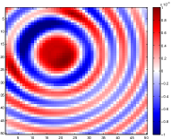
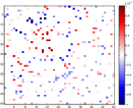
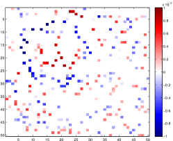
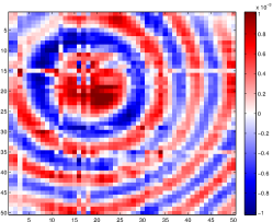
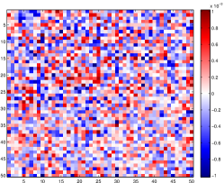
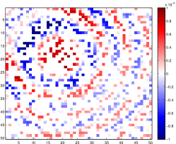
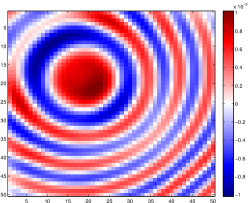
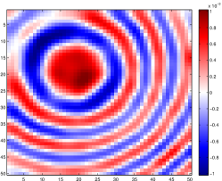
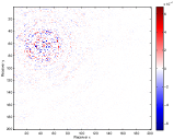
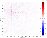
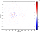
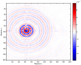
We consider the two sampling scenarios discussed in the previous section: we remove random points from the tensor, with results shown in Figure 5, and we remove random receivers from the tensor, with results shown in Figure 6. Here geomCG($r_{\text{leaf}}$) - $w$ denote the Tucker interpolation algorithm with rank $r_{\text{leaf}}$ in each mode and $w$ rank continuation steps, i.e., the approach proposed in [32]. We also let HT($r_{\text{leaf}},r_{x_{\text{src}}x_{\text{rec}}}$) denote the HT interpolation method with rank $r_{\text{leaf}}$ as in the Tucker interpolation and rank $r_{x_{\text{src}}x_{\text{rec}}}$ as the internal rank for the dimension tree. As is customary in the seismic literature, we measure recovery quality in terms of SNR, namely

$$\text{SNR}(\mathbf{X},\mathbf{D})=-20\log_{10}\left(\dfrac{\|\mathbf{X}_{\Omega^{c}}-\mathbf{D}_{\Omega^{c}}\|}{\|\mathbf{D}_{\Omega^{c}}\|}\right)\text{dB},$$

where $\mathbf{X}$ is our interpolated signal, $\mathbf{D}$ is our reference solution, and $\Omega^{c}=[n_{src}]\times[n_{src}]\times[n_{rec}]\times[n_{rec}]\setminus\Omega$. As we can see in Figure 5, the HT formulation is able to take advantage of low-rank separability of the seismic volume to produce a much higher quality solution than that of the Tucker tensor completion. The rank continuation scheme does not seem to be improving the recovery quality of the Tucker solution to the same degree as in [32], although it does seem to mitigate some of the overfitting errors for geomCG($30$). We display slices for fixed source coordinates and varying receiver coordinates in Figure 5 for randomly missing points and Figure 6 for randomly missing receivers. By exploiting the low-rank structure of the HT format compared to the Tucker format, we are able to achieve much better results than Tucker tensor completion, especially for the realistic case of missing receiver samples.

In all instances for these experiments, the HT tensor completion outperforms the conventional Tucker approach both in terms of recovery quality and recovery speed. We note that geomCG does not scale as well computationally as our HT algorithm for $d>3$, as the complexity analysis in [32] predicts. As such, we only consider the HT interpolation for the next sections, where we will solve the tensor completion problem for much larger data volumes.

(a) True data

(b) Input data $b=P_{\Omega}\mathbf{X^{*}}$

(c) HT(30,80) - SNR $30.5$ dB

(d) geomCG(20)-0 - SNR $29.4$ dB

Figure 5. Reconstruction results for 90% missing points, best results for geomCG and HTOpt.

(a) 90% missing receivers

(b) HT(20,20) - SNR $7.04$ dB

(c) geomCG(20)-0 - SNR $-1.92$ dB

(d) 70% missing receivers

(e) HT(20,20) - SNR $20.4$ dB

(f) geomCG(30)-5 - SNR $16.8$ dB

Figure 6. Reconstruction results for sampled receiver coordinates, best results for geomCG and HTOpt. (a-c) 90% missing receivers. (d-f): 70% missing receivers.

	Single reflector data - sampling percentage (missing points)
	10%		30%		50%
	SNR [dB]	time [s]	SNR [dB]	time [s]	SNR [dB]	time [s]
geomCG(20) - 0	28.5	1023	30.5	397	30.7	340
geomCG(30) - 0	-6.7	1848	21.8	3621	31.5	2321
geomCG(30) - 5	16.1	492	13.8	397	15.5	269
HTOpt(20,60)	30.1	83	30.4	59	30.4	57
HTOpt(20,80)	30.3	121	30.8	75	30.8	53
HTOpt(30,80)	31.6	196	32.9	133	33.1	114

Table 1. Reconstruction results for single reflector data - missing points - mean SNR over 5 random training sets

	Single reflector data - sampling percentage (missing receivers)
	10%		30%		50%
	SNR [dB]	time [s]	SNR [dB]	time [s]	SNR [dB]	time [s]
geomCG(20) - 0	-5.1	899	9.9	898	18.5	891
geomCG(30) - 0	-3.6	1796	-4.7	1834	6.1	1802
geomCG(30) - 5	-6.4	727	11.1	670	14.2	356
HTOpt(20,20)	6.1	111	19.8	101	20.1	66
HTOpt(30,20)	2.8	117	18.1	109	19.8	94
HTOpt(30,40)	0.0	130	13.4	126	21.6	108

Table 2. Reconstruction results for single reflector data - missing receivers - mean SNR over 5 random training test sets

6.3. Performance

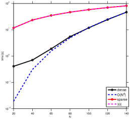
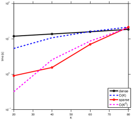
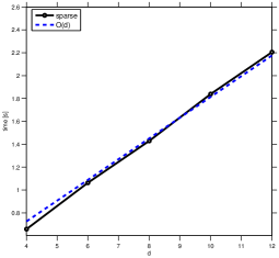
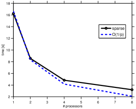
We investigate the empirical performance scaling of our approach as $N,d,K,$ and $|\Omega|$ increase, as well as the number of processors for the parallel case, in Figure 7 and Figure 8. Here we denote the use of Algorithm 1 as the “dense” case and Figure 2 as the “sparse” case. We run our optimization code in Steepest Descent mode with a single iteration for the line search, and average the running time over $10$ iterations and $5$ random problem instances. Our empirical performance results agree very closely with the theoretical complexity estimates, which are $O(N^{d}K)$ for the dense case and $O(|\Omega|dK^{3})$ for the sparse case. Our parallel implementation for the sparse case scales very close to the theoretical time $O(1/\text{\# processors})$.

(a) Fixed $K,d$, varying $N$, $|\Omega|=1000N$

(b) Fixed $N,d,|\Omega|$, varying $K$

Figure 7. Dense & sparse objective, gradient performance.

(a) Fixed $N,K,|\Omega|$, varying $d$

(b) Fixed $N,K,d,\Omega$, varying number of processors

Figure 8. Sparse objective, gradient performance.

6.4. Synthetic BG Compass data

This data set was provided to us by BG and consists of 5D data generated from an unknown synthetic model. Here $n_{src}=68$ and $n_{rec}=401$ and we extract frequency slices at 4.86 Hz, 7.34 Hz, and 12.3 Hz. On physical grounds, we expect a slower decay of the singular values at higher frequencies and thus the problem is much more difficult at 12.3 Hz compared to 4.86 Hz.

At these frequencies, the data has relatively low spatial frequency content in the receiver coordinates, and thus we subsample the receivers by a factor of $2$ to $n_{rec}=201$, for the purposes of speeding up the overall computation and ensuring that the intermediate vectors in the optimization are able to fit in memory. Our overall data volume has dimensions $\mathbf{D}\in\mathbb{R}^{68\times 68\times 201\times 201}$.

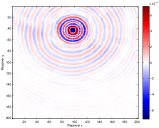
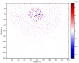
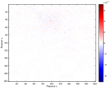
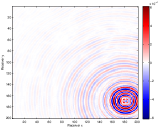
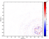
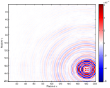
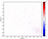
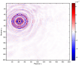
We randomly remove varying amounts of receivers from this reduced data volume and interpolate using 50 iterations of the GN method discussed earlier. We display several recovered slices for fixed source coordinates and varying receiver coordinates (so-called common source gathers in seismic terminology) in Figure 9.

We summarize our recovery results for tensor completion on these data sets from missing receivers in Table 3 and the various recovery parameters we use in Table 4. When the subsampling rate is extremely high (90% missing receivers in these examples), the recovery can suffer from overfitting issues, which leads to spurious artifacts in the recovered volume and lower SNRs overall. Using the Gramian-based regularization method discussed earlier, we can mitigate some of those artifacts and boost recovered SNRs, as seen in Figure 10.

7. Conclusions and discussion

In this work we have developed the algorithmic components to solve optimization problems on the manifold of fixed-rank Hierarchical Tucker tensors. By exploiting this manifold structure, we solve the tensor completion problem where the tensors of interest exhibit low-rank behavior. Our algorithm is computationally efficient because we mostly rely on operations on the small HT parameter space. The manifold optimization itself guarantees that we do not run into convergence issues, which arise when we ignore the quotient structure of the HT format. Our application of this framework to seismic examples confirms the validity of our new approach and outperforms existing Tucker-based approaches for large data volumes. To stabilize the recovery for high subsampling ratios, we introduced an additional regularization term that exploits properties of the Gramian matrices without the need to compute SVDs in the ambient space.

While the method clearly performs well on large-scale problems, there are still a number of theoretical questions regarding the performance of this approach. In particular, the generalization of matrix completion recovery guarantees to the HT format remains an open problem. As in many alternative approaches to matrix/tensor completion, the selection of the rank parameters and regularization parameters remain challenging both theoretically and from a practical point of view. However, the paper clearly illustrates that the HT format is a viable option to represent and complete high-dimensional data volumes in a computationally feasible manner.

8. Acknowledgements

We would like to thank the sponsors of the SINBAD consortium for their continued support. We would also like to thank the BG Group for providing us with the Compass data set.

Frequency	% Missing	Train SNR (dB)	Test SNR (dB)	Runtime (s)
4.86 Hz	25%	21.2	21	4033
	50%	21.3	20.9	4169
	75%	21.5	19.9	4333
	90%	19.9	10.4	4679
	$90\%^{*}$	$20.8^{*}$	$13.0^{*}$	5043
7.34 Hz	25%	17.3	17.0	4875
	50%	17.4	16.9	4860
	75%	17.7	16.5	5422
	90%	16.6	9.82	4582
	$90\%^{*}$	$16.6^{*}$	$10.5^{*}$	4947
12.3 Hz	25%	14.9	14.2	5950
	50%	15.2	13.8	7083
	75%	15.8	9.9	7387
	90%	13.9	5.39	4578
	$90\%^{*}$	$14^{*}$	$6.5^{*}$	4966

Table 3. HT Recovery results - randomly missing receivers. Starred quantities are computed with regularization.

Frequency	$k_{x_{src}x_{rec}}$	$k_{x_{src}}$	$k_{x_{rec}}$	HT-SVD SNR (dB)
4.86 Hz	150	68	120	21.1
7.34 Hz	200	68	120	17.0
12.3 Hz	250	68	150	13.9

Table 4. HT parameters for each data set and the corresponding SNR of the HT-SVD approximation of each data set. The 12.3 Hz data is of much higher rank than the other two data sets and thus is much more difficult to recover.

(a) True Data

(b) Subsampled Data

(c) Interpolated Data - SNR 20 dB

(d) Difference

(e) True Data

(f) Subsampled Data

(g) Interpolated Data - SNR 17.7 dB

(h) Difference

(i) True Data

(j) Subsampled Data

(k) Interpolated Data - SNR 11.2 dB

(l) Difference

Figure 9. 75% missing receivers, fixed source coordinates. Top: 4.68 Hz, Middle: 7.34 Hz, Bottom: 12.3 Hz.

(a) True Data

(b) Subsampled Data

(c) No Regularization - SNR 10.4 dB

(d) Regularization - SNR 13.9 dB

Figure 10. Regularization reduces some of the spurious artifacts and reduces overfitting in the case where there is very little data. 4.86 Hz data, 90% missing receivers.

Appendix A Adjoint multilinear operators

To derive expressions for the adjoint derivatives, we first consider the general multilinear product

$$A_{1}\times_{1}A_{2}\times_{2}\dots A_{d}\times_{d}\mathbf{B}\in\mathbb{R}^{m_{1}\times...\times m_{d}}$$

with $A_{i}\in\mathbb{R}^{m_{i}\times n_{i}}$ and $\mathbf{B}\in\mathbb{R}^{n_{1}\times n_{2}\times...\times n_{d}}$. Now, let $P_{i}$ be the linear operator that fixes each $A_{j}$ for $j\neq i$ in the above expression, i.e.,

$$P_{i} :\mathbb{R}^{m_{i}\times n_{i}}\to\mathbb{R}^{m_{1}\times...\times m_{d}}$$

$$P_{i}(C) :=A_{1}\times_{1}A_{2}\times_{2}\dots A_{i-1}\times_{i-1}C\times_{i}A_{i+1}\times_{i+1}\dots A_{d}\times_{d}\mathbf{B}.$$

In matricized form, this operator can be written as

$$(P_{i}(C))^{([d]\setminus i)}=CB^{(i)}(A^{T}_{d}\otimes A^{T}_{d-1}\otimes\dots\otimes A^{T}_{i+1}\otimes A^{T}_{i-1}\otimes\dots A_{1}^{T})$$

Taking the inner product of the matrix $(P_{i}(C)^{([d]\setminus i)}$ and a tensor $\mathbf{Y}$ matricized along the $i$th mode yields

$$\langle P_{i}(C)^{[d]\setminus i},Y^{(i)}\rangle =\text{tr}(CB^{(i)}(A^{T}_{d}\otimes A^{T}_{d-1}\otimes\dots\otimes A^{T}_{i+1}\otimes A^{T}_{i-1}\otimes\dots A_{1}^{T})(Y^{(i)})^{T})$$

$$=\langle C,Z\rangle$$

where $Z=Y^{(i)}(A_{d}\otimes A_{d-1}\otimes\dots\otimes A_{i+1}\otimes A_{i-1}\otimes\dots A_{1})(B^{(i)})^{T}$.

We note that $(A_{d}\otimes A_{d-1}\otimes\dots\otimes A_{i+1}\otimes A_{i-1}\otimes\dots A_{1})(B^{(i)})^{T}$ is the matricized form of

$$\mathbf{W}=A_{1}^{T}\times_{1}A_{2}^{T}\times_{2}\dots A_{i-1}^{T}\times_{i-1}I_{m_{i}}\times_{i}A_{i+1}^{T}\times_{i+1}\dots A_{d}^{T}\times_{d}\mathbf{B}$$

along the modes $[d]\setminus i$, and that $Y^{(i)}W^{([d]\setminus i)}$ is the tensor contraction $\langle\mathbf{Y},\mathbf{W}\rangle_{([d]\setminus i),([d]\setminus i)}$. It follows that the adjoint of the operator $P_{i}(C)$ in the standard Euclidean inner product is given by

$$P_{i}^{*}(\mathbf{Y})=\langle A_{1}^{T}\times_{1}A_{2}^{T}\times_{2}\dots A_{i-1}^{T}\times_{i-1}I_{m_{i}}\times_{i}A_{i+1}^{T}\times_{i+1}\dots A_{d}^{T}\times_{d}\mathbf{Y},\mathbf{B}\rangle_{([d]\setminus i),([d]\setminus i)}.$$

Likewise, for the linear operator

$$P_{\mathbf{B}}(\mathbf{C}):=A_{1}\times_{1}\dots A_{d}\times_{d}\mathbf{C}$$

we find that its adjoint is given by

$$P^{*}_{\mathbf{B}}(\mathbf{Y})=A_{1}^{T}\times_{1}\dots A_{d}^{T}\times_{d}\mathbf{Y}.$$

Appendix B Proof of Proposition 3

Proof.

It is easy to see that the first point in Definition 7 is satisfied, since for $X\in\text{St}(n,p)$, $\operatorname*{\text{\rm{qf}}}(X)=X$

Let $x=(U_{t},\mathbf{B}_{t})\in\operatorname*{\mathcal{M}}$ and $\eta=(\delta U_{t},\mathbf{\delta B_{t}})\in\mathcal{T}_{x}\operatorname*{\mathcal{M}}$. To avoid notational overload, we use the slight abuse of notation that $B_{t}:=B_{t}^{(1,2)}$ for $t\neq\operatorname*{t_{\text{root}}}$.

Let $s\in[0,t)\mapsto x(s)$ be a curve in the parameter space $\operatorname*{\mathcal{M}}$ with $x(0)=x$ and $x^{\prime}(0)=\eta$ and
$x(s)=(U_{t}(s),B_{t}(s))$ and $x^{\prime}(s)=(\delta U_{t}(s),\delta B_{t}(s))$.

Then we have that, in Kronecker form,

$$DR_{x}(0_{x})[\eta]=\begin{cases}\frac{d}{ds}\operatorname*{\text{\rm{qf}}}(x(s)_{t})\big{|}_{s=0}&\text{if }t\in L\\ \frac{d}{ds}\operatorname*{\text{\rm{qf}}}((R_{t_{r}}(s)\otimes R_{t_{l}}(s))(x(s)_{t})\big{|}_{s=0}&\text{if }t\not\in\operatorname*{t_{\text{root}}}\cup L\\ \frac{d}{ds}(R_{t_{r}}(s)\otimes R_{t_{l}}(s))(x(s)_{t})\big{|}_{s=0}&\text{if }t=\operatorname*{t_{\text{root}}}\end{cases}$$

The fact that $DR_{x}(0_{x})[\eta]_{t}=\delta U_{t}$ for $t\in L$ follows from Example 8.1.5 in [1].

To compute $DR_{x}(0_{x})[\eta]_{t}$ for $t\not\in L\cup\operatorname*{t_{\text{root}}}$, we first note the formula from [1]

(23) $$D\operatorname*{\text{\rm{qf}}}(Y)[U]=\operatorname*{\text{\rm{qf}}}(Y)\rho_{\text{skew}}(\operatorname*{\text{\rm{qf}}}(Y)^{T}U(\operatorname*{\text{\rm{qf}}}(Y)^{T}Y)^{-1})+(I-\operatorname*{\text{\rm{qf}}}(Y)\operatorname*{\text{\rm{qf}}}(Y)^{T})U(\operatorname*{\text{\rm{qf}}}(Y)^{T}Y)^{-1}$$

where $Y\in\mathbb{R}^{n\times k}_{*}$, $U\in T_{Y}\mathbb{R}_{*}^{n\times k}\simeq\mathbb{R}^{n\times k}$ and $\text{qf}(Y)$ is the Q-factor of the QR-decomposition of $Y$.

Therefore, if we set $Z(s)=(R_{t_{r}}(s)\otimes R_{t_{l}}(s))(x(s)_{t})$, where $R_{t}(s)$ is the $R$-factor of the QR-decomposition of the matrix associated to node $t$, we have

$$Z^{\prime}(0)=[(R^{\prime}_{t_{r}}(0)\otimes I_{k_{l}})+(I_{k_{r}}\otimes R^{\prime}_{t_{l}}(0)]B_{t}+\delta B_{t}$$

As a result of the discussion in Example 8.1.5 in [1], since $R_{t}(0)=I_{k_{t}}$ we have that

$$R^{\prime}_{t}(0)=\begin{cases}\rho_{UT}(U_{t}^{T}\delta U_{t})&\text{ for }t\in L\\ \rho_{UT}(B_{t}^{T}\delta B_{t})&\text{ for }t\not\in L\cup\operatorname*{t_{\text{root}}}\end{cases}$$

where $\rho_{UT}(A)$ is the projection onto the upper triangular term of the unique decomposition of a matrix into the sum of a skew-symmetric term and an upper triangular term.

Since $U_{t}\in\text{St}(n_{t},k_{t})$ and $B_{t}\in\text{St}(k_{t_{l}}k_{t_{r}},k_{t})$, in light of the fact that for $X\in St(n,k)$,

$$T_{X}St(n,k)=\{X\Omega+X^{\perp}K:\Omega=-\Omega^{T}\},$$

then $X^{T}\delta X$ is skew symmetric, for any tangent vector $\delta X$, which implies that $\rho_{UT}(X^{T}\delta X)$ is zero.

It follows that $R^{\prime}_{t}(0)=0$ for all $t\in T\setminus\operatorname*{t_{\text{root}}}$, and therefore

$$Z^{\prime}(0)=\delta B_{t}$$

from which we immediately obtain

$$DR_{x}(0_{x})[\eta]_{t}=\delta B_{t}\quad\text{for }t\not\in L\cup\operatorname*{t_{\text{root}}}$$

A similar approach holds when $t=\operatorname*{t_{\text{root}}}$, and therefore, $R_{x}(\eta)$ is a retraction on $\operatorname*{\mathcal{M}}$. ∎

Appendix C Square-root based retraction

Another straightforward projection onto the orthonormal parameter space is immediate from the remark that for a general full-rank $n\times p$ matrix $X$, with $n>p$, the matrix $X(X^{T}X)^{-1/2}$ is an orthonormal basis for the column space of $X$. In Algorithm 8, we only need to compute the eigenvalue decomposition of a $k_{t}\times k_{t}$ matrix, which may be done more efficiently than computing the QR-factorization of a $k_{t_{l}}k_{t_{r}}\times k_{t}$ matrix in some instances.

Algorithm 8 Square-root-based orthogonalization

0:  $x=(U_{t},\mathbf{B}_{t})$ unorthogonalized

  for  $t\in L$  do

     $M_{t}=U_{t}^{T}U_{t}$

     Compute the eigenvalue decomposition of $M_{t}$, $M_{t}=V_{t}D_{t}V_{t}^{T}$

     $U^{\prime}_{t}\leftarrow U_{t}M_{t}^{-1/2}$

  end for

  for  $t\in T\setminus L$, visiting children before their parents  do

     $C_{t}\leftarrow(M_{t_{l}}^{1/2}\times_{1}M_{t_{r}}^{1/2}\times_{2}\mathbf{B}_{t})^{(1,2)}$

     if $t=\operatorname*{t_{\text{root}}}$ then

        $B^{\prime}_{t}\leftarrow(C_{t})_{(1,2)}$

     else

        Compute the eigenvalue decomposition of $C_{t}^{T}C_{t}$, $C_{t}^{T}C_{t}=V_{t}D_{t}V_{t}^{T}$

        $B^{\prime}_{t}\leftarrow(C_{t}(C_{t}^{T}C_{t})^{-1/2})_{(1,2)}$

     end if

  end for

  return  $x^{\prime}=(U^{\prime}_{t},B^{\prime}_{t})$ in OHT

References

- Absil et al. [2008] P.A. Absil, R. Mahony, and R. Sepulchre. Optimization algorithms on matrix manifolds. Princeton Univ Press, 2008.
- Acar et al. [2011] Evrim Acar, Daniel M Dunlavy, and Tamara G Kolda. A scalable optimization approach for fitting canonical tensor decompositions. Journal of Chemometrics, 25(2):67–86, 2011.
- Bader et al. [2012] B. W. Bader, T. G. Kolda, et al. Matlab tensor toolbox version 2.5. http://www.sandia.gov/~tgkolda/TensorToolbox/, January 2012.
- Ballani et al. [2011] J. Ballani, L. Grasedyck, and M. Kluge. Black box approximation of tensors in hierarchical tucker format. Linear Algebra and its Applications, 2011.
- Ballani and Grasedyck [2013] Jonas Ballani and Lars Grasedyck. Tree adaptive approximation in the hierarchical tensor format. Preprint, 141, 2013.
- Cagliari et al. [2012] Francesca Cagliari, Barbara Di Fabio, and Claudia Landi. The natural pseudo-distance as a quotient pseudo-metric, and applications. AMS Acta, Universita di Bologna, 3499, 2012.
- Cai et al. [2010] Jian-Feng Cai, Emmanuel J Candès, and Zuowei Shen. A singular value thresholding algorithm for matrix completion. SIAM Journal on Optimization, 20(4):1956–1982, 2010.
- Candès and Recht [2009] E.J. Candès and B. Recht. Exact matrix completion via convex optimization. Foundations of Computational mathematics, 9(6):717–772, 2009.
- Candès and Tao [2010] Emmanuel J Candès and Terence Tao. The power of convex relaxation: Near-optimal matrix completion. Information Theory, IEEE Transactions on, 56(5):2053–2080, 2010.
- Carroll and Chang [1970] J. Carroll and J. Chang. Analysis of individual differences in multidimensional scaling via an n-way generalization of “eckart-young” decomposition. Psychometrika, 35:283–319, 1970. ISSN 0033-3123. URL http://dx.doi.org/10.1007/BF02310791. 10.1007/BF02310791.
- Da Silva and Herrmann [2013] Curt Da Silva and Felix J. Herrmann. Hierarchical tucker tensor optimization - applications to tensor completion. In 10th international conference on Sampling Theory and Applications (SampTA 2013), pages 384–387, Bremen, Germany, July 2013.
- De Lathauwer et al. [2000] L. De Lathauwer, B. De Moor, and J. Vandewalle. A multilinear singular value decomposition. SIAM Journal on Matrix Analysis and Applications, 21(4):1253–1278, 2000.
- De Silva and Lim [2008] V. De Silva and L.H. Lim. Tensor rank and the ill-posedness of the best low-rank approximation problem. SIAM Journal on Matrix Analysis and Applications, 30(3):1084–1127, 2008.
- Demanet [2006] Laurent Demanet. Curvelets, Wave Atoms, and Wave Equations. PhD thesis, California Institute of Technology, 2006.
- [15] M. P. Friedlander E. van den Berg. Spot – a linear-operator toolbox. URL http://www.cs.ubc.ca/labs/scl/spot/.
- Eldén and Savas [2009] Lars Eldén and Berkant Savas. A newton-grassmann method for computing the best multilinear rank-(r_1, r_2, r_3) approximation of a tensor. SIAM Journal on Matrix Analysis and applications, 31(2):248–271, 2009.
- Gandy et al. [2011] S. Gandy, B. Recht, and I. Yamada. Tensor completion and low-n-rank tensor recovery via convex optimization. Inverse Problems, 27(2):025010, 2011.
- Grasedyck [2010] L. Grasedyck. Hierarchical singular value decomposition of tensors. SIAM Journal on Matrix Analysis and Applications, 31(4):2029–2054, 2010.
- Grasedyck et al. [2013a] Lars Grasedyck, Melanie Kluge, and Sebastian Krämer. Alternating directions fitting (adf) of hierarchical low rank tensors. Preprint, 149, 2013a.
- Grasedyck et al. [2013b] Lars Grasedyck, Daniel Kressner, and Christine Tobler. A literature survey of low-rank tensor approximation techniques. GAMM-Mitteilungen, 36(1):53–78, 2013b.
- Hackbusch and Kühn [2009] W. Hackbusch and S. Kühn. A new scheme for the tensor representation. Journal of Fourier Analysis and Applications, 15(5):706–722, 2009.
- Harshman [1970] R.A. Harshman. Foundations of the parafac procedure: models and conditions for an" explanatory" multimodal factor analysis. 1970.
- Holtz et al. [2012a] Sebastian Holtz, Thorsten Rohwedder, and Reinhold Schneider. The alternating linear scheme for tensor optimization in the tensor train format. SIAM Journal on Scientific Computing, 34(2):A683–A713, 2012a.
- Holtz et al. [2012b] Sebastian Holtz, Thorsten Rohwedder, and Reinhold Schneider. On manifolds of tensors of fixed tt-rank. Numerische Mathematik, 120(4):701–731, 2012b.
- Huang et al. [2014] Bo Huang, Cun Mu, Donald Goldfarb, and John Wright. Provable low-rank tensor recovery. 2014.
- Khoromskij [2011] B.N. Khoromskij. Tensor-structured numerical methods in scientific computing: Survey on recent advances. Chemometrics and Intelligent Laboratory Systems, 2011.
- Kolda and Bader [2009a] Tamara G Kolda and Brett W Bader. Tensor decompositions and applications. SIAM review, 51(3):455–500, 2009a.
- Kolda and Bader [2009b] T.G. Kolda and B.W. Bader. Tensor decompositions and applications. SIAM review, 51(3):455–500, 2009b.
- Kreimer and Sacchi [2012a] N. Kreimer and M.D. Sacchi. Tensor completion via nuclear norm minimization for 5d seismic data reconstruction. In SEG Technical Program Expanded Abstracts 2012, pages 1–5. Society of Exploration Geophysicists, 2012a.
- Kreimer and Sacchi [2012b] Nadia Kreimer and Mauricio D Sacchi. A tensor higher-order singular value decomposition for prestack seismic data noise reduction and interpolation. Geophysics, 77(3):V113–V122, 2012b.
- Kressner and Tobler [2013] D. Kressner and C. Tobler. htucker - a matlab toolbox for tensors in hierarchical tucker format. http://sma.epfl.ch/~anchpcommon/publications/htucker.pdf, 2013.
- Kressner et al. [2013] D. Kressner, M. Steinlechner, and B. Vandereycken. Low-rank tensor completion by riemannian optimization. 2013.
- Lubich et al. [2013] Christian Lubich, Thorsten Rohwedder, Reinhold Schneider, and Bart Vandereycken. Dynamical Approximation by Hierarchical Tucker and Tensor-Train Tensors. SIAM Journal on Matrix Analysis and Applications, 34(2):470–494, April 2013.
- Mishra and Sepulchre [2013] B. Mishra and R. Sepulchre. R3mc: A riemannian three-factor algorithm for low-rank matrix completion. arXiv.org, June 2013.
- Mu et al. [2013] Cun Mu, Bo Huang, John Wright, and Donald Goldfarb. Square deal: Lower bounds and improved relaxations for tensor recovery. arXiv preprint arXiv:1307.5870, 2013.
- Oymak et al. [2012] Samet Oymak, Amin Jalali, Maryam Fazel, Yonina C Eldar, and Babak Hassibi. Simultaneously structured models with application to sparse and low-rank matrices. arXiv preprint arXiv:1212.3753, 2012.
- Shi and Shen [2005] Z J Shi and J Shen. New Inexact Line Search Method for Unconstrained Optimization. Journal of Optimization Theory and Applications, 127(2):425–446, November 2005.
- Shi [2004] Zhen-Jun Shi. Convergence of line search methods for unconstrained optimization. Applied Mathematics and Computation, 157(2):393–405, 2004.
- Signoretto et al. [2011] M. Signoretto, R. Van de Plas, B. De Moor, and J. AK Suykens. Tensor versus matrix completion: a comparison with application to spectral data. Signal Processing Letters, IEEE, 18(7):403–406, 2011.
- Tobler [2012] C. Tobler. Low Rank Tensor Methods for Linear Systems and Eigenvalue Problems. PhD thesis, ETH Zürich, 2012.
- Uschmajew [2012] A. Uschmajew. Local convergence of the alternating least squares algorithm for canonical tensor approximation. SIAM Journal on Matrix Analysis and Applications, 33(2):639–652, 2012.
- Uschmajew and Vandereycken [2013] A. Uschmajew and B. Vandereycken. The geometry of algorithms using hierarchical tensors. Linear Algebra and its Applications, 439(1):133–166, July 2013.