Detecting edge degeneracy in interacting topological insulators through entanglement entropy

Abstract

The existence of degenerate or gapless edge states is a characteristic feature of topological insulators, but is difficult to detect in the presence of interactons. We propose a new method to obtain the degeneracy of the edge states from the perspective of entanglement entropy, which is very useful to identify interacting topological states. Employing the determinant quantum Monte Carlo technique, we investigate the interaction effect on two representative models of fermionic topological insulators in one and two dimensions, respectively. In the two topologically nontrivial phases, the edge degeneracies are reduced by interactions but remain to be nontrivial.

I Introduction

Topologically nontrivial states of matter are a central topic of condensed matter physics, which are classified to two categories according to their ground state entanglement properties. The long-range entangled topological state, often named topologically ordered state, is characterized by the ground state degeneracy on a closed manifold Wen and Niu (1990); the short-range entangled topological insulator can be characterized by its edge degeneracy on an open boundary. (Below we use the term topological insulator to represent the general short-range entangled topological states protected by certain symmetries Schnyder et al. (2008); *Gu2009, not just for the time-reversal invariant $\mathcal{Z}_{2}$ topological insulators Hasan and Kane (2010); *Qi2011.) For a non-interacting topological insulator, edge degeneracy comes directly from the zero energy edge mode, which is protected by its bulk topological property through the bulk-edge correspondence Hatsugai (1993); *Ryu2002; Qi et al. (2006) .

However, the single-particle picture of the edge zero modes does not apply in interacting systems. The usual bulk-edge correspondence should be understood as the relation between bulk topological property and the many-body ground state degeneracy on the edge . The concept of edge degeneracy originates from the study of critical quantum systems Affleck and Ludwig (1991). Recently, it was also generalized to topologically ordered systems Wang and Wen (2012), and has been widely used for the classification of interacting topological insulators Fidkowski and Kitaev (2011); *Qi2013; *Yao2013; Tang and Wen (2012). In this article, we will apply this concept to the systems of interacting topological insulators.

Edge properties are important for the study of interaction effects in topological insulators. The first problem studied is the edge stability in the time-reversal invariant topological insulators in the presence of strong interactions Wu et al. (2006); *Xu2006. Because the edge is gapless, interaction effects on the edge are more prominent than those in the bulk, which can lead to edge instabilities while maintain the time-reversal invariance in the bulk. The above picture has also been confirmed in quantum Monte Carlo (QMC) simulations Zheng et al. (2011); Hohenadler et al. (2011). In recent years, interacting topological insulators have been intensively studied Wu et al. (2006); *Xu2006; Hohenadler et al. (2011); Zheng et al. (2011); Yu et al. (2011); Raghu et al. (2008); *Dzero2010; *Shitade2009; *Zhang2012; *Rachel2010; *Varney2010; *Yuan2012, which have also been classified according to different symmetries Fidkowski and Kitaev (2011); *Qi2013; *Yao2013; Tang and Wen (2012); Chen et al. (2011); *Turner2011; *Lu2012; *Gu2012; *Wang2013; Tang and Wen (2012). For the time-reversal invariant topological insulators, the $\mathcal{Z}_{2}$ index can be formulated in terms of the single-particle Green’s functions Wang et al. (2010); *Wang2011; *Wang2012, which has been calculated based on both analytic and numeric methods Manmana et al. (2012); Wang et al. (2012); *Araujo2013; Hung et al. (2013); *Lang2013.

On the other hand, quantum entanglement provides a particular perspective to investigate quantum many-body physics Amico et al. (2008); *Eisert2010. Entanglement entropy measures non-local correlations between part $A$ and the rest of the system denoted as part $B$. Entanglement entropy can be defined as the von Neumann entropy

$$S_{v}=-\mathrm{Tr}[\rho_{A}\ln\rho_{A}],$$ (1)

based on the reduced density matrix $\rho_{A}=\mathrm{Tr}_{B}(\rho_{A\cup B})$. For systems characterized by short-range entanglement, entanglement entropy obeys an area law: It is proportional to the area/length of the boundary, i.e., the entanglement cut. However, in the quantum critical region, entanglement entropy shows a logarithmic dependence on the subsystem size due to the divergence of coherence length Vidal et al. (2003); *Calabrese2004. In topologically ordered systems with long-range entanglements, a negative sub-leading term appears termed as topological entanglement entropy Kitaev and Preskill (2006); *Levin2006, which depends on the degeneracy of ground states. Topological entanglement entropy has been used to identify different topological orders in quantum spin liquid systems Zhang et al. (2011); *Zhang2012a; Yan et al. (2011); *Jiang2012; *Jiang2012a. For short-range entangled topological insulators, the single-particle entanglement spectrum Li and Haldane (2008) is found to exhibit a “zero mode”-like behavior Ryu and Hatsugai (2006); Fidkowski (2010) in the non-interacting case. However, interaction invalids such a single-particle picture, and thus a more delicate method is required to describe interacting topological insulators.

In this article, we propose a method to determine the edge degeneracy using entanglement entropy. A quantity termed edge entanglement entropy $S_{n,\rm edge}$ (defined in Eq. 5) is employed to measure edge degeneracy for both non-interacting and interacting topological insulators. This work is motivated by a recently developed algorithm using the fermionic determinant QMC to calculate the Renyi entanglement entropy Grover (2013); *Assaad2013

$$S_{n}=-\frac{1}{n-1}\ln\mathrm{Tr}[\rho_{A}^{n}].$$ (2)

We employ this algorithm to study edge degeneracy of fermionic interacting topological insulators by measuring $S_{2,\rm edge}$ in both one and two dimensional systems. Our methodology will be first explained by using the Su-Schrieffer-Heeger-Hubbard (SSHH) model Su et al. (1979). In the topologically nontrivial phase, the Hubbard $U$ reduces $S_{2,\rm edge}$ from $2\ln 2$ to $\ln 2$, corresponding to reducing edge degeneracy from $4$ to $2$ in the thermodynamic limit. In 2D, $S_{2,\rm edge}$ also contributes a sub-leading term to the entanglement entropy area law, as we observed in the Kane-Mele-Hubbard (KMH) model Kane and Mele (2005) for a cylindrical geometry. Moreover, $S_{2,\rm edge}$ shows even-odd dependence on the system size along the entanglement cut in agreement with the helical liquid behavior on the edge.

II The SSHH model

The 1D SSHH model is defined as

$$H_{\rm SSHH} = -\sum_{i=1,\sigma}^{2L}\left[t+\delta{t}(-1)^{i}\right]c_{i\sigma}^{\dagger}c_{i+1,\sigma}+H.c.$$ (3)

$$+\sum_{i=1}^{2L}\frac{U}{2}(n_{i}-1)^{2},$$

where $\sigma=\uparrow,\downarrow$; $n_{i}=\sum_{\sigma}c_{i\sigma}^{\dagger}c_{i\sigma}$,; $\delta{t}$ controls the hopping dimerization strength; $t$ is set $1$ below; $U$ is the Hubbard interaction.

At $U=0$, this model is well-known exhibiting two topologically distinct ground states, characterized by Berry phase $0$ ($\delta{t}>0$) and $\pi$ ($\delta{t}<0$), respectively. We use the convention that two sites $2i-1$ (odd) and $2i$ (even) are combined into one unit cell. The $\pi$-valued Berry phase guarantees the existence of one zero energy mode for each spin on each end Ryu and Hatsugai (2006) (inset of Fig. 1(a)) at $\delta{t}<0$. In order to study the entanglement entropy, the chain is divided into two parts $A$ and $B$: Using the truncated correlation matrix $\mathcal{C}_{ij,\sigma}=\langle c_{i\sigma}^{\dagger}c_{j\sigma}\rangle$ with $i,j\in A$, the Renyi entanglement entropy can be obtained Peschel (2003); *Cheong2004 as

$$S_{n}=-\frac{1}{n-1}\sum\ln f_{i\sigma}^{n},$$ (4)

where $f_{i\sigma}$ are eigenvalues of $\mathcal{C}_{ij,\sigma}$. $S_{2}$ is calculated under both the periodic boundary condition (PBC) and the open boundary condition (OBC), respectively, as plotted in Fig.  1(a). In partice, for $\delta{t}>0$, we choose $[1;L/2]$ as subsystem $A$ and $[L/2+1;L]$ as sublattice B for both OBC and PBC. In this case, all the cuts are at weak bonds. On the other hand, for $\delta{t}<0$, we use a different partition method such that the cuts are still at weak bonds. For the case of OBC, we choose $[1;L/2+1]$ and $[L/2+2;L]$ as subsystems A and B, respectively, while for the case of PBC, we choose $[2;L/2+1]$ and $[L/2+2;1]$ as subsystems A and B, respectively, such that again all the cuts are at weak bonds. Fig. 1(a) shows that neither PBC nor OBC gives quantized entanglement entropy because of the short-range entanglement near the cut to bipartite the system Ryu and Hatsugai (2006). Of course, that we can also choose the cuts on strong bonds and define the edge entanglement

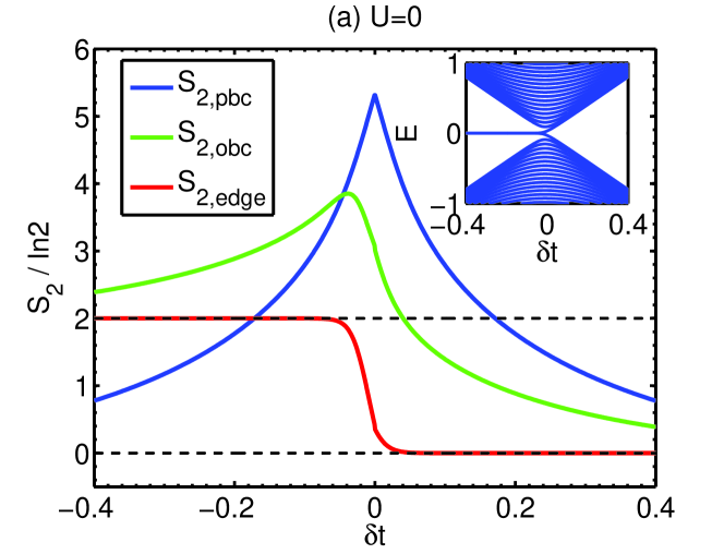
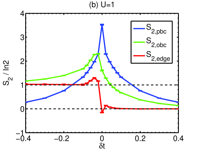
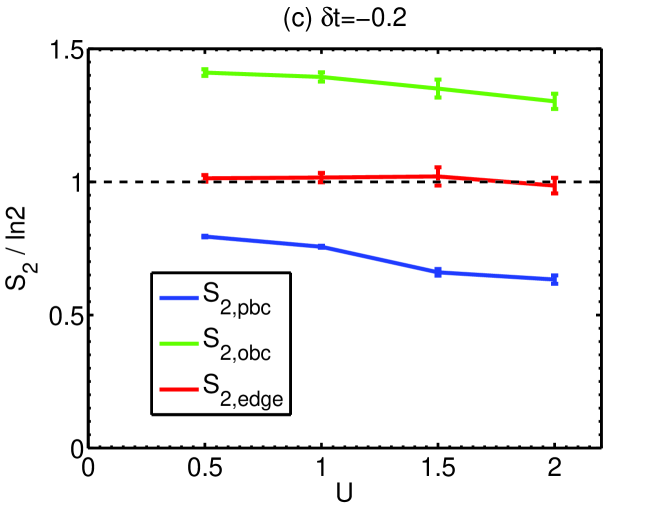
Figure 1: The 2nd order Renyi entanglement entropy of the 1D SSHH model. $S_{2,\rm pbc}$, $S_{2,\rm obc}$, and $S_{2,\rm edge}$ are plotted in (a) (U=0), (b) (U=1) as functions of $\delta{t}$, and in (c) ($\delta{t}=-0.2$) as functions of $U$. Parameter values for the QMC simulations are the projection time $\beta=120$ ($200$) for $U\geq 1$ ($U=0.5$) and the discrete time step $\Delta\tau=0.1$. The chain length is $L=100$ in (a), and $L=40$ in (b),(c).

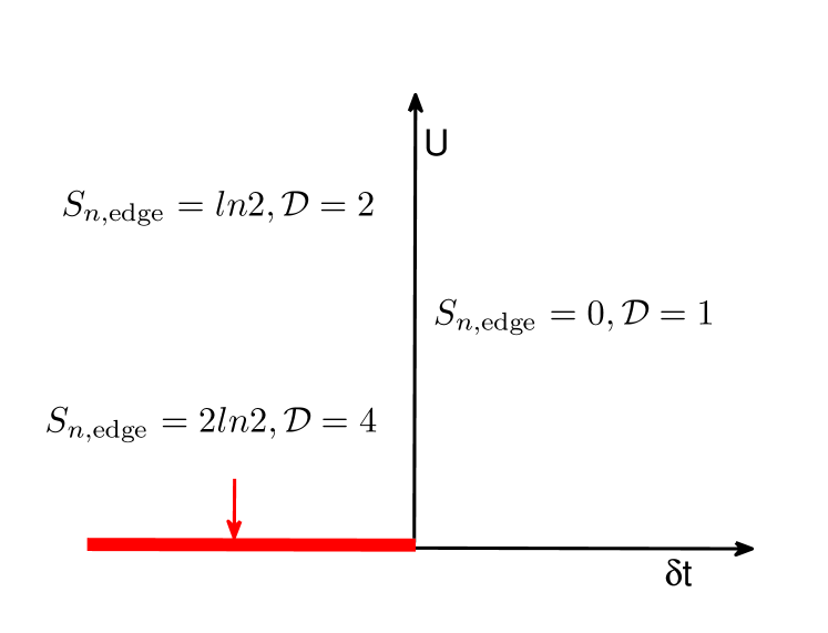
Figure 2: The phase diagram of the SSHH model determined from the edge entanglement entropy $S_{n,\rm edge}$ and edge degeneracy $\mathcal{D}$.

To extract the entanglement between two edges, we define the edge entanglement entropy as

$$S_{n,\rm edge}=S_{n,\rm obc}-\frac{S_{n,\rm pbc}}{2},$$ (5)

where half of $S_{n,\rm pbc}$ is subtracted because there are two cuts for defining entanglement in the case of PBC but only one in the case of OBC. This definition also applies for the interacting case. Eq. 5 measures the nonlocal entanglement between the edges. Although $n$ can be any integer number, we only consider the case of $n=2$ below because of the numerical convenience by QMC. Certainly we can also choose cuts on strong bonds and define $S_{n,edge}$ by subtraction accordingly, the results of the quantization of $S_{n,edge}$ remain robust.

The edge entanglement entropy exhibits a quantized behavior in two gapped phases. At $U=0$, Fig.  1 (a) shows $S_{2,\rm edge}=2\ln 2=\ln 4$ at $\delta{t}<0$ while $S_{2,\rm edge}=0$ at $\delta{t}>0$. This result can be understood as follows. For each spin component $\sigma$, two zero modes $\gamma_{(L,R)\sigma}$ at two ends are coupled through an effective hopping $t_{eff}\sim\exp(-\delta{t}L)$, and then the bonding state, $\frac{1}{\sqrt{2}}(\gamma_{L\sigma}^{\dagger}+\gamma_{R\sigma}^{\dagger})|0\rangle$, contributes a $\ln 2$ to $S_{n,\rm edge}$ in each spin component. More explicitly, this bonding edge states are occupied by both spin components, i.e., the two-particle edge states can be written as

$$\frac{1}{2}(\gamma_{L\uparrow}^{\dagger}\gamma^{\dagger}_{L\downarrow}+\gamma_{R\uparrow}^{\dagger}\gamma^{\dagger}_{R\downarrow}+\gamma_{L\uparrow}^{\dagger}\gamma^{\dagger}_{R\downarrow}+\gamma_{R\uparrow}^{\dagger}\gamma^{\dagger}_{L\downarrow})|0\rangle,$$ (6)

which clearly exhibit the $\ln 4$ contribution to the edge entanglement entropy.

Now let us consder to take the limit of $L\rightarrow+\infty$ in which $t_{eff}$ approaches to zero and the edge modes become exactly zero modes. Then each term in Eq. 6 corresponds to a zero mode for either edge. Say, after tracing out the degree of freedom on the right edge, we arrive at the zero modes at the left edge as $\gamma^{\dagger}_{L\uparrow}\gamma^{\dagger}_{L\downarrow}|0\rangle$, $|0\rangle$, $\gamma^{\dagger}_{L\uparrow}|0\rangle$, $\gamma^{\dagger}_{L\downarrow}|0\rangle$. Thus the above defined $S_{2,edge}$ can be used as a topological index, which corresponds to the thermodynamic entropy at zero temperature of one edge. This explains the relation between entanglement entropy and the ground state degeneracy $\mathcal{D}$ on one open end as

$$\ln\mathcal{D}=\lim_{L\to\infty}S_{n,\rm edge}(L),$$ (7)

which converges to the same value independent of $n$. It is sufficient to calculate $S_{2}$ to determine edge degeneracy. A similar quantity to Eq. 5 was used as a topological invariant to study 1D non-interacting $p$-wave superconductor Kim (2013). The physical meaning of this topological invariant becomes clear in our approach: it represents entanglement between two edges for a finite lattice size, and converges to edge degeneracy in the thermodynamic limit very quickly. Note that at the critical point $\delta{t}=0$, $S_{2,\rm edge}$ is negative and unquantized, in agreement with the “non-integer” edge degeneracy in critical quantum systems Affleck and Ludwig (1991).

Now let us turn on the Hubbard interaction $U$. We combine the zero temperature projector QMC Assaad and Evertz (2008) with the new developed algorithm to calculate $S_{2}$ Grover (2013) under PBC and OBC, respectively. Due to the particle-hole symmetry, the half-filled SSHH model is free of the sign problem, and thus the QMC simulation can be performed in a controllable way. The results of $S_{2}$ v.s. $\delta{t}$ at $L=40$ and $U=1$ are calculated and plotted in Fig. 1 (b). The behavior of $S_{2,\rm edge}$ is similar to the case of $U=0$ in Fig. 1 (a) except that its quantized value becomes $\ln 2$ when $\delta{t}<0$. At large values of $L$, $U\gg t_{eff}$, and thus the singlet ground state changes to

$$\frac{1}{\sqrt{2}}\left[\gamma_{L\uparrow}^{\dagger}\gamma_{R\downarrow}^{\dagger}-\gamma_{L\downarrow}^{\dagger}\gamma_{R\uparrow}^{\dagger}\right]|0\rangle,$$ (8)

leads to $S_{2,\rm edge}=\ln 2$. Again in the limit of $L\rightarrow+\infty$, the edge modes become exactly zero modes. If we trace out the right edge, the zero modes left at the left edge is $\gamma^{\dagger}_{\uparrow}|0\rangle$, and $\gamma^{\dagger}_{\downarrow}|0\rangle$, which means that edge degeneracy $D$ is reduced from $4$ to $2$ by the Hubbard $U$, i.e, the double and empty occupations of the edge states are projected out. Due to the exponential decay of $t_{eff}$, the finite-size effect of $S_{2,\rm edge}$ is weak. It converges to $\ln\mathcal{D}$ quickly even before $L$ goes large.

We have also calculated $S_{2,\rm pbc}$, $S_{2,\rm obc}$ and $S_{2,\rm edge}$ at different values of $U$ ranging from $0.5$ to $2$ as shown in Fig. 1 (c). $S_{2,\rm pbc}$ and $S_{2,\rm obc}$ are non-quantized, which decreases as increasing $U$ due to the suppression of charge fluctuations across the cuts. Nevertheless, $S_{2,\rm edge}$ is pinned at $\ln 2$ regardless of different values of $U$ due to the exponential suppression of $t_{eff}$. In Fig. 2, we set up the phase diagram of the SSHH model using $S_{n,\rm edge}$ and edge degeneracy. Similar phase diagram has been obtained by calculating the bulk topological number $\mathcal{Z}=0(2)$ for $\delta{t}>0(<0)$ using Green’s functions extracted from the density matrix renormalization group Manmana et al. (2012). Our study here further indicates the edge behavior: in the topologically nontrivial region, edge degeneracy is reduced from $4$ to $2$ by the Hubbard interaction Tang and Wen (2012) at half-filling.

When $U$ is large, the low energy physics of the SSHH model is described by the spin-$1/2$ Heisenberg-Peierls model $H=\sum_{i}J_{i}\vec{S}_{i}\cdot\vec{S}_{i+1}$, where $J_{i}=J$ or $J^{\prime}$ for the odd or even bond, respectively Wang et al. (2013). Our study shows that the cases of $J^{\prime}<J$ and $J^{\prime}>J$ belong to topologically distinct phases. At $J^{\prime}>J$, there is a free local moment at one end resulting in a double edge degeneracy. The transition occurs at $J=J^{\prime}$ consistent with the critical behavior of the spin $1/2$ Heisenberg model des Cloizeaux and Pearson (1962); Haldane (1983).

For the above results, the particle-hole symmetry gives rise to zero energy edges in non-interacting cases. The finite size effect couples the two edge states together and contributes to $S_{n,\rm edge}$. Even in the interacting case, our numeric simulations show that $S_{n,\rm edge}$ remains robust. When the particle-hole symmetry is gone, for the 1D case, both edge states are not at zero energy. They are either both occupied or empty, and thus $S_{n,\rm edge}$ will be reduced to zero. Nevertheless, our method still applies to the 2D Kane-Mele-Hubbard model because the chemical potential crosses the 1D band of edge states. The single particle states right at the chemical potential play the role of zero energy states.

III The KMH model

Next we move to 2D and investigate the KMH model on a honeycomb lattice defined as

$$H_{\rm KMH} = -\sum_{\langle i,j\rangle,\sigma}tc_{i\sigma}^{\dagger}c_{j\sigma}+\sum_{\langle\langle i,j\rangle\rangle,\sigma}i\lambda c_{i\sigma}^{\dagger}\sigma c_{j\sigma}$$ (9)

$$+\sum_{i}\frac{U}{2}(n_{i}-1)^{2},$$

where $\lambda$ is the next-nearest neighbor spin-orbit coupling; $\sigma=\uparrow,\downarrow$; again $t$ is set $1$. This model is free of the sign problem and has been investigated by the determinant QMC Zheng et al. (2011); Hohenadler et al. (2011). Along the $y$-direction (zigzag), the PBC is applied, and along the $x$-direction (armchair), both of the PBC and OBC are applied. The PBC and OBC correspond to the toric and cylindrical geometries, respectively. The lattice is divided into the subsystem $A$ with $1\leq x\leq L/2$ and the environment $B$ with $L/2+1\leq x\leq L$ for the study of entanglement entropy.

The QMC results of $S_{2,\rm pbc}$ and $S_{2,\rm obc}$ for the KMH model are shown in Fig. 3. $S_{2,\rm pbc}$ exhibits a standard area law, i.e., $S_{2,\rm pbc}\propto L_{y}$, while $S_{2,\rm obc}$ shows an even-odd oscillating behavior. Then $S_{2,\rm edge}=\ln 2$ and $0$ for even and odd values of $L_{y}$, respectively, as shown in the inset. On the other hand, $S_{2,\rm edge}$ can also be obtained by extrapolating $S_{2,\rm obc}(L_{y})$ for even values of $L_{y}$, in which $S_{2,\rm edge}$ appears as the sub-leading term of the area law as

$$S_{2,\rm obc}(L_{y})\approx\alpha L_{y}+S_{2,\rm edge}.$$ (10)

Such a sub-leading term is an analogy to the topological entanglement entropy in the long-range entangled topological orders Kitaev and Preskill (2006); *Levin2006; Zhang et al. (2011); *Zhang2012a; Yan et al. (2011); *Jiang2012; *Jiang2012a. We propose to use $S_{2,\rm edge}$ to characterize the short-range entangled topological insulators in 2D. Both topological entanglement entropy and $S_{2,\rm edge}$ are related to the ground state degeneracy, but account for bulk and edge states, respectively.

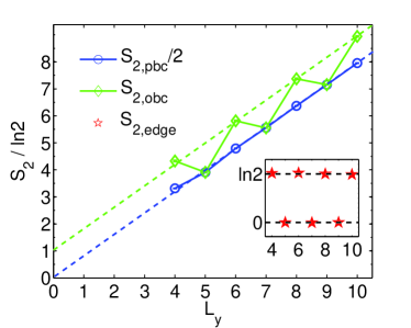
Figure 3: The 2nd order Renyi entanglement entropy of the KMH model v.s. $L_{y}$. $S_{2,\rm edge}$ is plotted in the inset. Parameter values are $U=1$, $\lambda=0.2$, $\beta=10L_{y}$, $\Delta\tau=0.1$, and $L_{x}=6$.

Next we explain the origin of the nonzero $S_{2,\rm edge}$ by analyzing the edge degeneracy. At $U=0$, such a behavior is a direct consequence of the zero-energy edge states, which has also been found in the Kitaev model Yao and Qi (2010), and non-interacting triplet topological superconductors Oliveira et al. (2013). In Fig. 4 (a), the energy spectrum with the open edges is plotted as a function of $k_{y}$ which is conserved due to the PBC along the $y$-direction. The edge zero mode is located at $k_{y}=\pi$, which is accessible for even values of $L_{y}$ but not for odd $L_{y}$, thus the many-body ground state degeneracy varies between $4$ and $1$ respectively.

At $U>0$, the above single-particle picture does not hold any more. Interaction effects have to be fully taken into account to investigate the many-body edge degeneracy. We use an effective edge helical liquid defined in momentum space Wu et al. (2006),

$$H_{hl} = \sum_{k,\sigma}\sigma v_{F}(k-\pi)c_{k\sigma}^{\dagger}c_{k\sigma}$$ (11)

$$+ \frac{U}{L_{y}}\sum_{kk^{\prime}q}c_{k+q\uparrow}^{\dagger}c_{k\uparrow}c_{k^{\prime}-q\downarrow}^{\dagger}c_{k^{\prime}\downarrow},$$

where $c_{k\sigma}^{\dagger}$ are creation operators of non-interacting edge states. The $y$-direction momenta $k=\frac{2\pi n}{L_{y}}$ ($n=0,1,\cdots,L_{y}-1$) are chosen only for edge states and satisfy $|v_{F}(k-\pi)|\leq\Lambda$ where $\Lambda$ is the energy cutoff. Since edge modes with different values of $k$ have different localization lengths, rigorously speaking, the interaction matrix elements for the edge modes are $k$-dependent even for the case of Hubbard model. Nevertheless, for simplicity, we neglect this dependence. In real calculations, we choose $\Lambda=\pi v_{F}/2=1$ without loss of generality. The number of momentum points for edge states within the cut off is denoted as $N_{k}$.

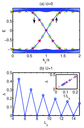
Figure 4: The helical edge behavior of the KMH model. (a) The single-particle energy spectra at $U=0$. Red and blue symbols mark the edge specta with even ($L_{y}=10$) and odd ($L_{y}=9$) values of $L_{y}$, respectively. (b) The many-body energy gap $\Delta$ v.s. $L_{y}$ for the effective model Eq. 11 with $U=1$ and $\Lambda=\pi v_{F}/2=1$. The inset plots $\Delta$ v.s. $1/L_{y}$ for only odd $L_{y}$.

Exact diagonalization method is employed to numerically solve the many-body edge energy levels at $L_{y}\leq 15$ ($N_{k}\leq 8$), and the energy gaps are plotted in Fig. 4 (b). For even $L_{y}$’s, $\Delta=0$ corresponds to a double degeneracy in agreement with the QMC result $S_{2,\rm edge}=\ln 2$; For odd $L_{y}$’s, the ground state has no degeneracy, thus $S_{2,\rm edge}=0$. Nevertheless, the gap decreases to zero as increasing $L_{y}$ as shown in the inset. This gapless behavior in the thermodynamic limit has been obtained from the bosonization analysis Wu et al. (2006), which shows that forward scattering does not open a gap in a helical liquid in the weak interacting regime.

IV Summary

We propose a quantized quantity of the edge entanglement entropy $S_{n,\rm edge}$ to determine edge degeneracy in topological insulators in the presence of interactions. Using the fermionic quantum Monte Carlo algorithm, $S_{n,\rm edge}$ is calculated for both the interacting 1D SSHH model and 2D KMH model. In topologically nontrivial phases of these models, the Hubbard $U$ suppresses the quantized values of $S_{2,\rm edge}$ from $2\ln 2$ in the non-interacting cases to its half value $\ln 2$. In 2D, such a nonzero $S_{n,\rm edge}$ also contributes a sub-leading term in the entanglement entropy area law for a cylindrical geometry.

Before closing this paper, some remarks are in order: (I) Our QMC calculations are only performed at small and medium $U$. When $U$ goes large, the QMC numeric error of entanglement entropy increases significantly Assaad et al. (2014). Significant numeric efforts are needed to obtain reliable entanglement entropy. Very recently, a new QMC algorithm using the replica technique was proposed for fermionic systems Broecker and Trebst (2014), which is more stable in the large $U$ regime and can be helpful to study the Mott transition regime in the future; (II) If the third nearest neighbor hopping is added to the KMH model, two Dirac nodes are produced at $k_{y}=0$ and $\pi$ respectively on an edge Hung et al. (2013). In this case, any small $U$ will gap out the edge states due to the Umklapp scattering Wu et al. (2006). Therefore, $S_{2,\rm edge}=0$ is expected to be consistent with the physical implication of the $\mathcal{Z}_{2}$ topological insulator. (III) We have seen that the above edge state entanglement is built up through the effective coupling $\sim\exp(-L_{x}/\xi)$ between two edges, in which $L_{x}$ is the width of the system, and $\xi$ is the typical localization length of the edge modes. On the other hand, for the 2D case, the length $L_{y}$ along the edge direction also gives another energy scale for the low energy edge excitations, which is $\sim 1/L_{y}$. When $\exp(-L_{x}/\xi)\ll 1/L_{y}$ (the regime we are interest), for the edge modes not right located at the Fermi energy, we can neglect their contributions to the total EE, and only need to consider the zero energy mode right at the Fermi energy. In this regime, our method applies.