Shape Profiles and Orientation Bias for
Weak and Strong Lensing Cluster Halos

Abstract

We study the intrinsic shape and alignment of isodensities of galaxy cluster halos extracted from the MultiDark MDR1 cosmological simulation. We find that the simulated halos, are extremely prolate on small scales, and increasingly spherical on larger ones. Due to this trend, analytical projection along the line of sight produces an overestimate of the concentration index as a decreasing function of radius, which we quantify by using both the intrinsic distribution of 3D concentrations ($c_{200}$) and isodensity shape on weak and strong lensing scales. We find this difference to be $\sim 18\%$ ($\sim 9\%$) for low (medium) mass cluster halos with intrinsically low concentrations ($c_{200}=1-3$), while we find virtually no difference for halos with intrinsically high concentrations. Isodensities are found to be fairly well-aligned throughout the entirety of the radial scale of each halo population. However, major axes of individual halos have been found to deviate by as much as $\sim 30^{\circ}$. We also present a value-added catalog of our analysis results, which we have made publicly available to download.

1. Introduction

Galaxy clusters represent the most massive of the virialized structures in the universe, whose development comes after billions of years of hierarchical merging of matter. Clusters offer us key insights into the structure formation process as predicted by the standard Lambda Cold Dark Matter ($\Lambda$CDM) cosmological paradigm (Corless & King, 2009; Ettori et al., 2009). Radial density profiles, mass functions, and the baryon mass fraction are all used to constrain cosmological parameters (Navarro et al., 2004; Voit, 2005; Diaferio et al., 2008; Allen et al., 2011), and rely on the accurate measurement of the distribution of mass within clusters, total mass, and proper characterization of halo substructure.

Gravitational lensing has proven an incredibly useful tool in creating detailed maps of projected density without requiring any assumptions regarding either a halo’s dynamical state or hydrostatic equilibrium of its gas. Recently, strong and weak gravitational lensing methods have been used side by side to constrain the distribution of mass on different scales within the same cluster lens (for Abell 1689 for example, see Broadhurst et al., 2005; Halkola et al., 2006; Deb et al., 2012).

Observations suggest that cluster halos exhibit triaxial geometry (see Limousin et al. 2013 for a general discussion) in the optical distribution of light (Carter & Metcalfe, 1980; Binggeli, 1982) in X-ray (Fabricant et al., 1985; Lau et al., 2012) and in weak (Evans & Bridle, 2009; Oguri et al., 2010, 2012) and strong lensing (Soucail et al., 1987). Observational evidence for triaxiality is matched by theory in large scale N-body simulations of structure formation, exhibiting a preference for prolateness over oblateness (Frenk et al., 1988; Dubinski & Carlberg, 1991; Warren et al., 1992; Cole & Lacey, 1996; Jing & Suto, 2002a; Hopkins et al., 2005; Bailin & Steinmetz, 2005; Kasun & Evrard, 2005; Paz et al., 2006; Allgood et al., 2006; Bett et al., 2007; Muñoz-Cuartas et al., 2011; Gao et al., 2012).

However, the over-simplification of the spherical halo approximation has serious consequences on their utility as cosmological probes. Of particular importance to cosmology is the concentration of the halo, $c_{200}$, a measure of how centrally concentrated the halo is. Qualitatively, the concentration describes the steepness of the inner density profile of the halo, where larger concentrations give rise to a steeper (“cuspier”) inner density profile, and conversely, smaller concentrations produce a more well-defined central core, indicating a shallower inner density profile. It has been shown through simulations that the concentration scales inversely with halo mass in the form of a power-law, and has also been more intuitively related to the formation time of a certain fraction of the mass of the main halo progenitor (Giocoli et al., 2012b).

A somewhat long-standing discrepancy between observations and what $\Lambda$CDM predicts is what is known as the over-concentration problem, wherein observed cluster concentrations are nearly twice what simulations predict (Broadhurst et al., 2008; Oguri et al., 2009). Bahé et al. (2012) have shown that when observed in near alignment with their major axes, weak lensing reconstructed concentrations are systematically larger by up to a factor of 2 for Millennium Simulation cluster halos. Similarly, Oguri & Blandford (2009) find in their semi-analytic study that the most massive triaxial halos ($\sim 10^{15}\mathrm{h}^{-1}\mathrm{M}_{\odot}$) produce the largest Einstein radii if they’re viewed preferentially along their major axes, thereby increasing their effectiveness as strong gravitational lenses. Through ray-tracing of high-resolution N-body simulations, Hennawi et al. (2007) have shown that strong lensing clusters tend to have their principle axes aligned along the line of sight. The projection bias due to triaxial halos associated with lensing methods has been fairly successful in describing much of the discrepancy between predictions and measurements. Giocoli et al. (2012a) have shown that knowledge of the elongation along the line of sight can help in correcting mass estimates, though a small negative bias remains in concentration.

Additional complications arise in this picture of cluster halos in that halo axis ratios change as a function of radius. Frenk et al. (1988) and Cole & Lacey (1996) found that simulation halos become more spherical towards the center, whereas Dubinski & Carlberg (1991), Warren et al. (1992), and Jing & Suto (2002a) have concluded the opposite. Nearly all are in agreement that there is good alignment between isodensity (or isopotential) surfaces on most scales. More recent work done by Hayashi et al. (2007) show that axis ratios of both isopotential and isodensity surfaces consistently increase with radius for seven galaxy-scale simulations.

Though lensing concentrations are systematically higher than their predicted values simply due to orientation bias, there are other reasons to believe that clusters identified by their strong lensing features are a biased population. For one, the most massive clusters are simply more effective gravitational lenses, preferentially sampling the highest region of the cluster mass hierarchy (Comerford & Natarajan, 2007).

Many studies have employed joint weak and strong lensing reconstruction techniques in order to probe much larger regions of the radial density profile. However, weak and strong lensing can sometimes independently produce vastly different results, and are rather sensitive to the a priori assumptions made regarding the distribution of mass within the cluster lens. Broadhurst et al. (2005) and Halkola et al. (2006) both find weak lensing concentrations to be much larger than ones produced by strong lensing of the well-known cluster Abell 1689, when a spherical model is used. Weak + strong lensing analyses of Abell 1689 have generally been in agreement with one another, however, concentrations remain inconsistent with what theory predicts (Clowe, 2003; Halkola et al., 2006; Limousin et al., 2007). Only when a triaxial halo model is employed do theory and observation come into agreement (Oguri et al. 2005; for a complete overview of the cluster Abell 1689, see $\S$5 of Limousin et al. 2013). The model assumptions and priors used in weak and strong lensing methods can produce large uncertainty in reconstructed parameters. However, physical features of the cluster halos, for example the combination of an orientation bias together with an intrinsic trend in halo shape as a function of radius could perhaps also lay at the heart of discrepancies of this nature, and work to diminish the accuracy of lensing techniques as stand-alone tools as well as joint techniques.

Lastly, ongoing baryonic physics within galaxy clusters (specifically cooling, star formation, and AGN feedback) has the potential to significantly alter the distribution of mass within clusters, and is absent from many simulations of structure formation. The lensing cross-section depends sensitively on the addition of baryons to cluster simulations, and can be boosted by a factor of a few (Puchwein et al., 2005; Wambsganss et al., 2008; Rozo et al., 2008). Studies which do not include AGN feedback suffer from over-cooling, and the addition of this component reduces the enhancement of the lensing cross-section to at most a factor of two (Mead et al., 2010). Killedar et al. (2012) find Einstein radii of clusters to be larger only by $5\%$ when AGN feedback is included for $z_{s}=2$ (increasing to $10-20\%$ for lower source redshifts).

In this paper we present a study of the shape and alignment of isodensity surfaces from simulated cluster halos of the MDR1 cosmological simulation (Prada et al., 2012) throughout a range of radial scales. Differences between the concentration parameter on weak and strong lensing scales will be quantified by the analytical projection of NFW halos, for the specific case that their major axes point along our line of sight. This paper is organized as follows. In section $\S$2, we discuss the extension of the spherical NFW model and present prolate spheroidal simplifications of halo properties upon projection of the 3D NFW profile along the line of sight. In $\S$3 we define our samples and methods we will use to analyze halo intrinsic properties. In $\S$4 we present our findings on weak and strong lensing scales within clusters, and discuss our results in $\S$5. And lastly, in $\S 6$ we add a general discussion of future work.

2. Projections of Triaxial NFW Halos

The Navarro-Frenk-White density profile (Navarro et al., 1996) has been shown to describe simulation halos over many decades of mass. The model in its simplest form contains two free parameters, $r_{s}$ and $c_{200}$ (implicitly in $\delta_{c_{200}}$; Equation 3):

$$\rho_{\mathrm{NFW}}(r)=\frac{\rho_{cr}\delta_{c_{200}}}{r/r_{s}(1+r/r_{s})^{2}}$$ (1)

The first parameter is the scale radius $r_{s}$, which describes the turning point of the profile - the point at which the slope of the logarithmic density is equal to -2. The second is the concentration, which we define as

$$c_{200}\equiv r_{200}/r_{s}$$ (2)

where $r_{200}$ is the radius at which the average density contained within it is a factor of 200 times larger than the critical density of the universe at the redshift of the halo. The characteristic overdensity of the cluster is defined in terms of the concentration in the following way:

$$\delta_{c_{200}}=\frac{200}{3}\frac{c_{200}^{3}}{\ln{(1+c_{200})}-\frac{c_{200}}{(1+c_{200})}}$$ (3)

Mass can now be defined in terms of $r_{200}$ and the cosmology-dependent critical density of the universe at the redshift of the halo.

$$M_{200}(z)=\frac{4}{3}\pi r_{200}^{3}\cdot 200\rho_{cr}(z)$$ (4)

The concentration is an important measurement, since it has been shown through simulations to scale inversely (though somewhat weakly) with the virial mass of the halo (Navarro et al., 1996; Bullock et al., 2001; Hennawi et al., 2007). More recent work done by Prada et al. (2012) has actually revealed a new flattening/upturn feature in the concentration-mass relationship for high redshift high mass halos in the Millennium-I and II, Bolshoi, and MultiDark simulations.

Simulations show that halos deviate from spherical symmetry by a considerable amount, with a preference for prolate over oblate spheroids. Doroshkevich (1970) has made the case that triaxial collapse is a necessary outcome of structure formation models which are seeded by Gaussian random initial conditions. The spherical NFW profile can be extended to accommodate triaxial halos by redefining the radial coordinate as an ellipsoidal coordinate:

$$\zeta^{2}=\frac{x^{2}}{c^{2}}+\frac{y^{2}}{b^{2}}+\frac{z^{2}}{a^{2}}$$ (5)

where $a,b,c$ are the semi-major, -intermediate, and -minor axes of the ellipsoidal shell under consideration. Each set of semi-axes is unique to a specific radial value within each halo by the relationship $abc=r^{3}$.

The projection of an arbitrary triaxial halo onto a 2-dimensional plane is a unique process. However, the reverse process is degenerate. To understand the limits of projection biases due to orientation, we simplify the generalized projection of triaxial halos found in Sereno et al. (2010a) assuming a prolate spheroidal geometry. The following observed (projected) parameters can be expressed in terms of the angle $\theta$ between the line-of-sight and the major axis of a prolate spheroid, as well as a single axial ratio intrinsic to the cluster (Table 1).

Table 1Prolate Spheroidal Geometry

Projected Quantity	Prolate Spheroidal Expression
$Q$	$\frac{q}{\sqrt{\sin^{2}{\theta}+q^{2}\cos^{2}{\theta}}}$
$R_{s}$	$\frac{q}{Q}r_{s}$
$\delta_{C}$	$\frac{Q^{2}}{q}\delta_{c}$

Shown here are the analytical expressions for projected quantities expressed in terms of intrinsic quantities and halo orientation used throughout this study. As a general rule, projected quantities will be capitalized while intrinsic quantities will not be.

3. Sample and Methods

3.1. Simulation Sample

We aim to quantify the effect which line-of-sight alignment of triaxial cluster halos has upon projected concentrations on both weak and strong lensing scales in the presence of slowly evolving isodensity shapes. We study clusters from the MDR1 cosmological simulation (Prada et al., 2012) of the MultiDark Project. MDR1 is a dark matter only simulation which uses $2048^{3}$ particles in a box 1 h^-1Gpc on a side. The mass of simulation particles is $8.721\times 10^{9}$ h^-1M_⊙, with a resolution of 7 h^-1kpc. The simulation uses results from WMAP5 as its cosmology and was run with the Adaptive-Refinement Tree (ART) code (Kravtsov et al., 1997).

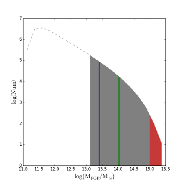
Figure 1.— Shown in black is the MDR1 mass function using the FOF algorithm. The gray shaded region shows the cluster halo regime. Overplotted are the low (blue), medium (green), and high (red) mass samples extracted from the database.

The MDR1 simulation database (Riebe et al., 2013) contains halo catalogs which are found using two different halo finding algorithms (“Bound Density Maximum” BDM, and “Friends-of-Friends” FOF) taken at 85 redshift snapshots. The masses of halos found through these two methods range from $1.7\times 10^{11}\mathrm{h}^{-1}\mathrm{M}_{\odot}$ - $1.6\times 10^{15}\mathrm{h}^{-1}\mathrm{M}_{\odot}$. We impose a lower cutoff in halo mass of $1\times 10^{13}\mathrm{h}^{-1}\mathrm{M}_{\odot}$ to mark the beginning of the cluster halo regime which are considered for this study. Figure 1 shows the mass function of the sample at redshift $z=0$.

In our study, three halo samples were extracted from the MDR1 FOF table (relative linking length of 0.17) of the MultiDark Database for further study. Smaller linking lengths (e.g. halo substructures) are available, however these were purposefully left out since it is beyond the scope of this study.

• Low Mass: $2.5-2.6\times 10^{13}\mathrm{h}^{-1}\mathrm{M}_{\odot}$ [6007 halos]

• Medium Mass: $1.0-1.1\times 10^{14}\mathrm{h}^{-1}\mathrm{M}_{\odot}$ [2905 halos]

• High Mass: $>1.0\times 10^{15}\mathrm{h}^{-1}\mathrm{M}_{\odot}$ [121 halos]

It should be noted here that our results are derived using one particular agglomerative, single-linkage clustering algorithm (FOF). Studies have been conducted which compare various halo-finding algorithms for simulation data (see Knebe et al. (2011) for a general review of such algorithms and how they perform in identifying structures from simulations). Despali et al. (2013) have shown that halo shape can depend upon the choice of method used to identify halos from the overall simulation volume.

3.2. Methods

Following, for example, (Warren et al., 1992; Shaw et al., 2006), we compute the moment of inertia tensor, from which we obtain the average shape of the halo at a given radius:

$$I_{ij}=\sum_{n=1}^{n=N}m_{p}(r_{i,n}-\bar{r_{i}})(r_{j,n}-\bar{r_{j}})$$ (6)

where $r_{i,n}$ is the coordinate of the $n^{th}$ particle in the $i^{th}$ direction (where $i,j\in{x,y,z}$), and $m_{p}$ is the mass of the simulation particle. Finding the eigenvalues and eigenvectors of $I$ can uniquely determine the orientation and axis ratios.

This method of determining shape has its drawbacks. Shaw et al. (2006), Jing & Suto (2002b), and Bailin & Steinmetz (2004) have all found that this approach often fails to converge in high resolution simulations with substantial substructure. Additionally, substructures of fixed mass will affect the components of the moment of inertia tensor on larger scales than it will on small scales. In order to correct for this, we apply a Gaussian weighting function, $w_{g}(\zeta)$, (to Equation 6) which matches both the shape and orientation of each bounding ellipsoid within the iterative process.

We find good convergence with this method for MDR1 halos. For our purposes, calculating the shape of each halo using the inertia tensor, with the addition of a triaxial, Gaussian weighting function, will be more than adequate to describe the macrostructure of the parent halo.

3.3. Non-Virialized Halos

Mergers are common physical processes in the formation of galaxy clusters (Press & Schechter, 1974; Bond et al., 1991; Lacey & Cole, 1993). Special care is taken to separate out halos which are better fit by more than one halo for each mass sample, since parameters like concentration and scale radius are only properly defined for a single halo profile. The Mean Shift clustering algorithm (Fukunaga & Hostetler, 1975) is used on low and medium mass clusters, while the K-Means (Hartigan & Wong, 1979) clustering algorithm is used for high mass halos.

The Mean Shift algorithm is a non-parametric algorithm which requires no initial guess for the number of clusters, making it ideal for handling clusters of arbitrary shape or number. It locates local density maxima and uses a tuning parameter to associate each particle’s membership to a corresponding maximum. Conversely, the K-Means algorithm necessarily requires k-clusters to group particles into. K-Means scales as $O(knT)$ (where $k$ is the number of clusters, $n$ is the number of points, and $T$ is the number of iterations) and therefore was chosen for the high mass sample of 121 halos.

Additionally, to prevent contamination of each sample by unrelaxed or actively merging structures which may be well-fit by a single model, halos are checked for virialization using the following method (Shaw et al., 2006):

$$\beta=\frac{2T_{0}-E_{s}}{W_{0}}+1$$ (7)

where $T_{0}$ is the total kinetic energy, $W_{0}$ is the total potential energy, and $E_{s}$ comes from the pressure of the outer perimeter of the halo, an important contribution which comes from the fact that cluster halos are not isolated systems. A cut is made at $\beta>-0.2$ in order to remove halos which have sufficient pressure at their virial radii, indicating that they are currently in a state of collapse (Shaw et al., 2006).

All analysis results for each cluster halo within this study have been stored in a downloadable database.

4. Results

Based upon the above criteria that a halo must be both virialized and best fit by a single component halo model, we find that $55.3\%$, $42.0\%$, and $17.4\%$ of halos in the low, medium, and high mass samples make it through our selection criteria. Additionally, nearly all of these cluster halos can be described as being prolate ellipsoids, becoming marginally more spherical with increasing distance from the cluster center (See Figure 2; See Table 2 for a summary of these shape results).

Table 2Cluster Halo Geometry

Radial Scale				Low	Medium	High
$0.5\cdot r_{200}$		$\bar{p}\pm\sigma_{p}$		$0.67\pm 0.15$	$0.62\pm 0.14$	$0.56\pm 0.13$
		$\bar{q}\pm\sigma_{q}$		$0.53\pm 0.12$	$0.49\pm 0.11$	$0.42\pm 0.06$
$r_{200}$		$\bar{p}\pm\sigma_{p}$		$0.71\pm 0.13$	$0.66\pm 0.13$	$0.54\pm 0.15$
		$\bar{q}\pm\sigma_{q}$		$0.57\pm 0.11$	$0.52\pm 0.10$	$0.42\pm 0.08$
$2\cdot r_{200}$		$\bar{p}\pm\sigma_{p}$		$0.69\pm 0.12$	$0.67\pm 0.12$	$0.54\pm 0.12$
		$\bar{q}\pm\sigma_{q}$		$0.55\pm 0.10$	$0.53\pm 0.10$	$0.43\pm 0.08$

Reported here are the sample mean (standard deviation) values of the semi-intermediate to semi-major axis ratio $p$, and semi-minor to semi-major axis ratio $q$ for each mass sample (virialized, non-mergers) at various physical scales of interest.

$\begin{array}[]{c}\includegraphics[scale={0.4}]{LMSingleVirialHalf.pdf}\end{array}$

Figure 2.— Shown above is the distribution of isodensity shapes for the low mass halo sample at a radial scale of $\sim 0.5r_{200}$. The green and blue shaded regions are the 1- and 2-$\sigma$ gaussian error ellipses, and red indicates the sample mean.

Intrinsic NFW concentrations are shown in Figure 3, and are consistent with those produced in previous simulations as well as previous studies of the MultiDark simulation (Prada et al., 2012). As expected, halo concentrations decrease with increasing halo mass. This concentration-mass relationship is generally fit with a power-law model which takes the form:

$$c_{200}=\frac{c_{0}}{\left(1+z\right)^{\beta}}\left(\frac{\mathrm{M}_{200}}{\mathrm{M}_{*}}\right)^{\alpha}$$ (8)

where for our sample $z=0$, and we use M${}_{*}=10^{14}\mathrm{h}^{-1}$M_⊙ (Figure 4). We first compute $r_{200}$ from the cumulative density profile of each halo, and thus establishing M₂₀₀. Next, by fitting NFW profiles to these density profiles we obtain concentration parameters. For MDR1 cluster halos, we find a concentration-mass relation of

$$c_{200}=\left(4.775\pm 0.022\right)\left(\frac{\mathrm{M}_{200}}{10^{14}\mathrm{h}^{-1}\mathrm{M}_{\odot}}\right)^{-0.056\pm 0.007}$$ (9)

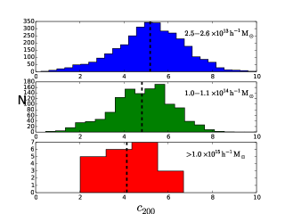
Figure 3.— Shown here are the distributions of intrinsic concentrations for all single virialized halos of each mass sample. From top to bottom: 1) Low Mass, 2) Medium Mass, and 3) High Mass.

From the intrinsic distributions of shape and concentration found for each sample population, we find that solely due to line-of-sight orientation, projected concentrations tend to be systematically higher by about $20\%-50\%$ for virialized, single model halos. Halos with intrinsically low concentrations have been found to suffer from a larger orientation bias $\sim 50\%$, whereas higher intrinsic concentrations tend to produce an over-concentration of $\sim 20\%$, albeit with much lower scatter. Additionally, this trend tends to flatten out with increasing distance from the cluster center. This means for a fixed halo concentration, inner regions of halos (those probed on or near strong lensing scales) will bias higher than outer regions of halos (those probed on weak lensing scales) if viewed along the major axis. This information is captured for relaxed, low mass halos (Figure 5; See also Table 3 for a complete summary).

The underlying cause for this mismatch in over-concentration between halos with intrinsically low and intrinsically high concentrations is due to the magnitude of the change in shape as a function of radius. Low concentration halos are shown to significantly change their shape between $0.5\cdot r_{200}$ and $r_{200}$, increasing in p and q, $81\%$ and $80\%$ of the time with median differences of $\Delta p=0.14$ and $\Delta q=0.11$ (Figure 6). Halos with high intrinsic concentrations increase in p and q $\sim 65\%$ of the time, however, the median value of the difference in axial ratio drops to $\sim 0.03$.

On the extreme end, we have shown that although a systematic bias exists, certain low concentration halos ($c_{200}\sim 1-3$) with extreme axis ratios can produce upwards of a factor of two higher in projected concentration on a case-by-case basis. This can be seen most notably in the low and medium mass samples at $r\sim 0.5\cdot r_{200}$.

Additionally, we also find that concentric ellipsoidal shells are well described as being coaxial with one another, that is to say there is insignificant amounts of twisting of isodensity surfaces for each mass population. Alignment becomes even better with increasing radius, where the misalignment is a maximum at the innermost radial value. It should be noted, however, that alignment results are expected to be biased low due to correlation between each ellipsoidal surface and ones interior to it. Though the aggregate shows relatively good alignment, it is again possible for individual cluster halos to produce significant ($\lesssim 30^{\circ}$) offsets between projected isodensities located at strong and weak lensing scales. This fact alone complicates things, however in the limit of large numbers of cluster halos, this effect should be minimal in biasing reconstructed concentrations for the population as a whole.

5. Summary and Conclusions

We have shown that relaxed MultiDark MDR1 simulation (FOF) cluster halos which are well described by a single NFW density profile are primarily prolate spheroidal in geometry and become increasingly more spherical with increasing radius from the cluster center of mass. Using shape on weak and strong lensing scales as well as derived concentrations, we analytically project these halos along the line of sight. In doing so, we find that low mass clusters are typically over-concentrated by about 56% and 20% at half $r_{200}$ for concentrations between 1-3 and 7-10, respectively. At $r_{200}$ this enhancement drops to 38% and 19%. What this tells us is that the average projected concentration differs by about 18% for halos with intrinsically low concentrations simply due to differences in halo geometry as a function of radius. Clusters which do not meet this criteria show the opposite trend in shape, becoming more prolate with increasing radius.

Strong lensing clusters are usually identified by their hard to miss tangential or radial arcs, and are expected to represent a biased population simply because large mass and alignment along the line of sight are key ingredients in producing large Einstein radii. If these lensing clusters are in fact preferentially aligned along the line of sight (and are relaxed), we would expect that all else being equal weak lensing reconstructions should under-estimate the concentration for a population of such objects.

Projection effects aside, additional complications arise in measuring halo concentration using strong and weak lensing. For example, halo substructure can play a significant role in altering the shape of the lens as seen by strong lensing (Meneghetti et al., 2007), along with massive objects unassociated with the halo which lay along the line of sight (Puchwein & Hilbert, 2009). Redlich et al. (2012) also find that cluster mergers bias high the distribution of Einstein Radii, highlighting another source of potential bias. The weak lensing signal can be diminished by things like atmospheric PSF, correlations in the orientation of background galaxies due to large scale structure, among the usual sources of uncertainty in measuring galaxy shapes (for a review of galaxy shape measurement and correlation of galaxy shapes, see Hoekstra & Jain 2008; for a discussion of cluster triaxiality and projections of large scale structure see Becker & Kravtsov 2011).

6. Future Work

An explicit prediction has been made regarding the discrepancy between projected halo concentrations of cluster halos on characteristic lensing scales. A natural next step would be to simulate the signal produced from gravitational lensing by conducting mock weak and strong lensing analyses. However, one would realistically need to include the effects of baryons. Additionally, we plan to summarize the current state of the field of galaxy cluster mass reconstructions in each of the methods used. In future work, we will aggregate all measured NFW mass/concentration pairs from these methods in order to shed light on potential systematic observational biases, particularly on strong and weak lensing scales.

It has yet to be determined if this effect manifests itself in a measurable way for the cluster halo population. Follow-up observations of strong lensing clusters could be proposed as a way of testing the veracity of this prediction. Knowing the intrinsic distribution of cluster concentrations is difficult if not impossible due to the degenerate nature of the reverse-projection process. However, the shape of the distribution of measured concentrations due to lensing could possibly contain hallmark characteristics which could indicate the level of line of sight biasing of the population. With this information known, ultimately a correction procedure could then be proposed.

7. Acknowledgements

This work was primarily supported by NSF Grant 0908307. AMG would also like to recognize Kristin Riebe for answering any questions he had regarding the MultiDark database and colleagues Justin Bird and Markus Rexroth for their time and feedback.

The MultiDark Database used in this paper and the web application providing online access to it were constructed as part of the activities of the German Astrophysical Virtual Observatory as result of a collaboration between the Leibniz-Institute for Astrophysics Potsdam (AIP) and the Spanish MultiDark Consolider Project CSD2009-00064. The Bolshoi and MultiDark simulations were run on the NASA’s Pleiades supercomputer at the NASA Ames Research Center. The MultiDark-Planck (MDPL) and the BigMD simulation suite have been performed in the Supermuc supercomputer at LRZ using time granted by PRACE.

Many plots in this work were generated by astroML (Vanderplas et al., 2012), a python module for machine learning, data mining, and visualization of astronomical datasets.

Appendix

The analytic form of the projected concentration is derived with the assumption that the surface mass density remains a constant (that is, the combination of shape and radial profile must change in such a way as to keep the original 2-dimensional distribution the same). We start with the scale convergence of a triaxial NFW halo as described in Sereno et al. (2010b):

$$\kappa_{s}=\frac{f_{geo}}{\sqrt{e_{P}}}\frac{\rho_{s}}{\Sigma_{cr}}r_{sP}$$ (10)

where $e_{P}$, $r_{sP}$, and $f_{geo}$ are the projected inverse axis ratio (the inverse of Equation 9), projected scale radius, and a geometric elongation parameter, respectively.

$$f_{geo}=\frac{e_{P}^{1/2}}{e_{\Delta}}$$ (11)

The inverse projected axis ratio of a 3-dimensional ellipsoid viewed at an arbitrary viewing angle has been worked out by Binggeli (1980) to be

$$e_{P}=\sqrt{\frac{j+l+\sqrt{(j-l)^{2}+4k^{2}}}{j+l-\sqrt{(j-l)^{2}+4k^{2}}}}$$ (12)

where the intrinsic halo geometry (q is the semi-minor to semi-major axis ratio; p is the semi-intermediate to semi-major axis ratio) and viewing angle are input into:

$$j=q^{2}\sin^{2}\theta+p^{2}\sin^{2}\phi\cos^{2}\theta+\cos^{2}\phi\cos^{2}\theta$$ (13)

$$k=p^{2}\cos^{2}\phi+\sin^{2}\phi$$

$$l=\left(1-p^{2}\right)\sin\phi\cos\phi\cos\theta$$

The elongation parameter is defined in the following way:

$$e_{\Delta}=\left(\frac{e_{P}}{e_{1}e_{2}}\right)^{1/2}f^{3/4}$$ (14)

$$f=e_{1}^{2}\sin^{2}\theta\sin^{2}\phi+e_{2}^{2}\sin^{2}\theta\cos^{2}\phi+\cos^{2}\theta$$ (15)

Remembering that the scale density $\rho_{s}$ is

$$\rho_{s}=\rho_{cr}\delta_{c}$$ (16)

allows us to associate the extra geometric factor of $1/e_{\Delta}$ in the scale convergence expression with the overdensity.

$$\delta_{C}=\frac{1}{e_{\Delta}}\delta_{c}$$ (17)

$$\frac{C^{3}}{\log{\left(1+C\right)}-\frac{C}{1+C}}=\frac{1}{e_{\Delta}}\frac{c^{3}}{\log{\left(1+c\right)}-\frac{c}{1+c}}$$ (18)

The extra geometric factor can be expressed in terms of the prolate spheroidal projected axis ratio $Q$, a function of the intrinsic axis ratio q, and the angle between the major axis and the line-of-sight. Above, we have conclude that the assumption of prolateness is proven to be a reasonable one, thus the surplus in concentration can be completely expressed in terms of prolate spheroidal .

$$\frac{1}{e_{\Delta}}=\frac{Q^{2}}{q}$$ (19)

Table 3Concentration Enhancements

Radial Scale		Low Mass		Medium Mass
	$c_{200}$	$\bar{\Delta}_{c_{200}}\pm\sigma_{\Delta}$	$c_{200}$	$\bar{\Delta}_{c_{200}}\pm\sigma_{\Delta}$
$0.5\cdot r_{200}$	$[1-3]$	$1.56\pm 0.29$	$[1-3]$	$1.52\pm 0.25$
	$[7-10]$	$1.20\pm 0.07$	$[6-9]$	$1.26\pm 0.09$
$r_{200}$	$[1-3]$	$1.38\pm 0.16$	$[1-3]$	$1.43\pm 0.15$
	$[7-10]$	$1.19\pm 0.09$	$[6-9]$	$1.24\pm 0.09$
$1.5\cdot r_{200}$	$[1-3]$	$1.30\pm 0.12$	$[1-3]$	$1.34\pm 0.11$
	$[7-10]$	$1.17\pm 0.07$	$[6-9]$	$1.22\pm 0.09$
$2\cdot r_{200}$	$[1-3]$	$1.28\pm 0.11$	$[1-3]$	$1.31\pm 0.10$
	$[7-10]$	$1.18\pm 0.07$	$[6-9]$	$1.23\pm 0.09$

Average Concentration Enhancement ($\Delta_{c_{200}}\equiv C_{200}/c_{200}$) on Weak and Strong Lensing Scales for Low and Medium Mass Samples.

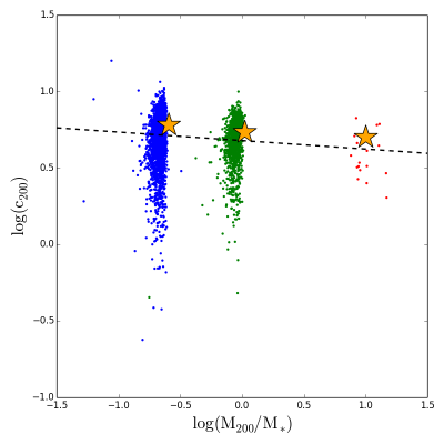
Figure 4.— Shown here is the intrinsic concentration-mass relationship for the MDR1 cosmological simulation run. Orange stars represent values of concentration from the analytical expression found in Prada et al. (2012) at redshift $z=0$ for values of halo mass corresponding to the sample used in this study.

$\begin{array}[]{cc}\includegraphics[scale={0.475}]{LMSingleVirialHalfConcsLOS.pdf}&\includegraphics[scale={0.475}]{LMSingleVirialFullConcsLOS.pdf}\end{array}$

Figure 5.— Shown here are concentration enhancements against intrinsic halo concentrations for line-of-sight oriented halos for the low mass, single-model, relaxed halo population. In the left (right) panel, we show the population at $\sim 0.5\cdot r_{200}$ ($\sim 1\cdot r_{200}$). Overplotted are the mean and standard deviation of low ($1\leq c_{200}\leq 3$) and high ($7\leq c_{200}\leq 10$) concentration halos for comparison.

$\begin{array}[]{ccc}\includegraphics[scale={0.3}]{p_low_1to3_half_full.png}&\includegraphics[scale={0.3}]{q_low_1to3_half_full.png}&\includegraphics[scale={0.3}]{pq_low_1to3_half_full_diff.png}\\ \includegraphics[scale={0.3}]{p_low_7to10_half_full.png}&\includegraphics[scale={0.3}]{q_low_7to10_half_full.png}&\includegraphics[scale={0.3}]{pq_low_7to10_half_full_diff.png}\end{array}$

Figure 6.— Halos with intrinsically low concentrations exhibit a much larger change in shape as a function of radius. Upper left and middle: Normalized distributions of axial ratios p and q for low-mass, low-concentration (1-3) halos at half $r_{200}$ (blue) and $r_{200}$ (green). Bottom left and middle: The distributions of axial ratios p and q for low-mass, high-concentration (7-10) halos at half $r_{200}$ and $r_{200}$. Upper right, (Lower right): Distributions of the differences in axial ratios p (purple) and q (orange) for low-concentration (high-concentration) low-mass cluster halos.

References

- Allen et al. (2011) Allen, S. W., Evrard, A. E., & Mantz, A. B. 2011, ARA&A, 49, 409
- Allgood et al. (2006) Allgood, B., Flores, R. A., Primack, J. R., et al. 2006, MNRAS, 367, 1781
- Bahé et al. (2012) Bahé, Y. M., McCarthy, I. G., & King, L. J. 2012, MNRAS, 421, 1073
- Bailin & Steinmetz (2004) Bailin, J., & Steinmetz, M. 2004, ApJ, 616, 27
- Bailin & Steinmetz (2005) —. 2005, ApJ, 627, 647
- Becker & Kravtsov (2011) Becker, M. R., & Kravtsov, A. V. 2011, ApJ, 740, 25
- Bett et al. (2007) Bett, P., Eke, V., Frenk, C. S., et al. 2007, MNRAS, 376, 215
- Binggeli (1980) Binggeli, B. 1980, A&A, 82, 289
- Binggeli (1982) —. 1982, A&A, 107, 338
- Bond et al. (1991) Bond, J. R., Cole, S., Efstathiou, G., & Kaiser, N. 1991, ApJ, 379, 440
- Broadhurst et al. (2005) Broadhurst, T., Takada, M., Umetsu, K., et al. 2005, ApJ, 619, L143
- Broadhurst et al. (2008) Broadhurst, T., Umetsu, K., Medezinski, E., Oguri, M., & Rephaeli, Y. 2008, ApJ, 685, L9
- Bullock et al. (2001) Bullock, J. S., Kolatt, T. S., Sigad, Y., et al. 2001, MNRAS, 321, 559
- Carter & Metcalfe (1980) Carter, D., & Metcalfe, N. 1980, MNRAS, 191, 325
- Clowe (2003) Clowe, D. 2003, in Astronomical Society of the Pacific Conference Series, Vol. 301, Matter and Energy in Clusters of Galaxies, ed. S. Bowyer & C.-Y. Hwang, 271
- Cole & Lacey (1996) Cole, S., & Lacey, C. 1996, MNRAS, 281, 716
- Comerford & Natarajan (2007) Comerford, J. M., & Natarajan, P. 2007, MNRAS, 379, 190
- Corless & King (2009) Corless, V. L., & King, L. J. 2009, MNRAS, 396, 315
- Deb et al. (2012) Deb, S., Morandi, A., Pedersen, K., et al. 2012, ArXiv e-prints, arXiv:1201.3636
- Despali et al. (2013) Despali, G., Tormen, G., & Sheth, R. K. 2013, MNRAS, 431, 1143
- Diaferio et al. (2008) Diaferio, A., Schindler, S., & Dolag, K. 2008, Space Sci. Rev., 134, 7
- Doroshkevich (1970) Doroshkevich, A. G. 1970, Astrophysics, 6, 320
- Dubinski & Carlberg (1991) Dubinski, J., & Carlberg, R. G. 1991, ApJ, 378, 496
- Ettori et al. (2009) Ettori, S., Morandi, A., Tozzi, P., et al. 2009, A&A, 501, 61
- Evans & Bridle (2009) Evans, A. K. D., & Bridle, S. 2009, ApJ, 695, 1446
- Fabricant et al. (1985) Fabricant, D., Rybicki, G., & Gorenstein, P. 1985, in X-ray Astronomy ’84, ed. M. Oda & R. Giacconi, 381–386
- Frenk et al. (1988) Frenk, C. S., White, S. D. M., Davis, M., & Efstathiou, G. 1988, ApJ, 327, 507
- Fukunaga & Hostetler (1975) Fukunaga, K., & Hostetler, L. 1975, Information Theory, IEEE Transactions on, 21, 32
- Gao et al. (2012) Gao, L., Navarro, J. F., Frenk, C. S., et al. 2012, MNRAS, 425, 2169
- Giocoli et al. (2012a) Giocoli, C., Meneghetti, M., Ettori, S., & Moscardini, L. 2012a, MNRAS, 426, 1558
- Giocoli et al. (2012b) Giocoli, C., Tormen, G., & Sheth, R. K. 2012b, MNRAS, 422, 185
- Halkola et al. (2006) Halkola, A., Seitz, S., & Pannella, M. 2006, MNRAS, 372, 1425
- Hartigan & Wong (1979) Hartigan, J. A., & Wong, M. A. 1979, Journal of the Royal Statistical Society. Series C (Applied Statistics), 28, 100
- Hayashi et al. (2007) Hayashi, E., Navarro, J. F., & Springel, V. 2007, MNRAS, 377, 50
- Hennawi et al. (2007) Hennawi, J. F., Dalal, N., Bode, P., & Ostriker, J. P. 2007, ApJ, 654, 714
- Hoekstra & Jain (2008) Hoekstra, H., & Jain, B. 2008, Annual Review of Nuclear and Particle Science, 58, 99
- Hopkins et al. (2005) Hopkins, P. F., Bahcall, N. A., & Bode, P. 2005, ApJ, 618, 1
- Jing & Suto (2002a) Jing, Y. P., & Suto, Y. 2002a, ApJ, 574, 538
- Jing & Suto (2002b) —. 2002b, ApJ, 574, 538
- Kasun & Evrard (2005) Kasun, S. F., & Evrard, A. E. 2005, ApJ, 629, 781
- Killedar et al. (2012) Killedar, M., Borgani, S., Meneghetti, M., et al. 2012, MNRAS, 427, 533
- Knebe et al. (2011) Knebe, A., Knollmann, S. R., Muldrew, S. I., et al. 2011, MNRAS, 415, 2293
- Kravtsov et al. (1997) Kravtsov, A. V., Klypin, A. A., & Khokhlov, A. M. 1997, ApJS, 111, 73
- Lacey & Cole (1993) Lacey, C., & Cole, S. 1993, MNRAS, 262, 627
- Lau et al. (2012) Lau, E. T., Nagai, D., Kravtsov, A. V., Vikhlinin, A., & Zentner, A. R. 2012, ApJ, 755, 116
- Limousin et al. (2013) Limousin, M., Morandi, A., Sereno, M., et al. 2013, Space Sci. Rev., 177, 155
- Limousin et al. (2007) Limousin, M., Richard, J., Jullo, E., et al. 2007, ApJ, 668, 643
- Mead et al. (2010) Mead, J. M. G., King, L. J., Sijacki, D., et al. 2010, MNRAS, 406, 434
- Meneghetti et al. (2007) Meneghetti, M., Argazzi, R., Pace, F., et al. 2007, A&A, 461, 25
- Muñoz-Cuartas et al. (2011) Muñoz-Cuartas, J. C., Macciò, A. V., Gottlöber, S., & Dutton, A. A. 2011, MNRAS, 411, 584
- Navarro et al. (1996) Navarro, J. F., Frenk, C. S., & White, S. D. M. 1996, ApJ, 462, 563
- Navarro et al. (2004) Navarro, J. F., Hayashi, E., Power, C., et al. 2004, MNRAS, 349, 1039
- Oguri et al. (2012) Oguri, M., Bayliss, M. B., Dahle, H., et al. 2012, MNRAS, 420, 3213
- Oguri & Blandford (2009) Oguri, M., & Blandford, R. D. 2009, MNRAS, 392, 930
- Oguri et al. (2010) Oguri, M., Takada, M., Okabe, N., & Smith, G. P. 2010, MNRAS, 405, 2215
- Oguri et al. (2005) Oguri, M., Takada, M., Umetsu, K., & Broadhurst, T. 2005, ApJ, 632, 841
- Oguri et al. (2009) Oguri, M., Hennawi, J. F., Gladders, M. D., et al. 2009, ApJ, 699, 1038
- Paz et al. (2006) Paz, D. J., Lambas, D. G., Padilla, N., & Merchán, M. 2006, MNRAS, 366, 1503
- Prada et al. (2012) Prada, F., Klypin, A. A., Cuesta, A. J., Betancort-Rijo, J. E., & Primack, J. 2012, MNRAS, 423, 3018
- Press & Schechter (1974) Press, W. H., & Schechter, P. 1974, ApJ, 187, 425
- Puchwein et al. (2005) Puchwein, E., Bartelmann, M., Dolag, K., & Meneghetti, M. 2005, A&A, 442, 405
- Puchwein & Hilbert (2009) Puchwein, E., & Hilbert, S. 2009, MNRAS, 398, 1298
- Redlich et al. (2012) Redlich, M., Bartelmann, M., Waizmann, J.-C., & Fedeli, C. 2012, A&A, 547, A66
- Riebe et al. (2013) Riebe, K., Partl, A. M., Enke, H., et al. 2013, Astronomische Nachrichten, 334, 691
- Rozo et al. (2008) Rozo, E., Nagai, D., Keeton, C., & Kravtsov, A. 2008, ApJ, 687, 22
- Sereno et al. (2010a) Sereno, M., Jetzer, P., & Lubini, M. 2010a, MNRAS, 403, 2077
- Sereno et al. (2010b) Sereno, M., Lubini, M., & Jetzer, P. 2010b, A&A, 518, A55
- Shaw et al. (2006) Shaw, L. D., Weller, J., Ostriker, J. P., & Bode, P. 2006, ApJ, 646, 815
- Soucail et al. (1987) Soucail, G., Fort, B., Mellier, Y., & Picat, J. P. 1987, A&A, 172, L14
- Vanderplas et al. (2012) Vanderplas, J., Connolly, A., Ivezić, Ž., & Gray, A. 2012, in Conference on Intelligent Data Understanding (CIDU), 47 –54
- Voit (2005) Voit, G. M. 2005, Reviews of Modern Physics, 77, 207
- Wambsganss et al. (2008) Wambsganss, J., Ostriker, J. P., & Bode, P. 2008, ApJ, 676, 753
- Warren et al. (1992) Warren, M. S., Quinn, P. J., Salmon, J. K., & Zurek, W. H. 1992, ApJ, 399, 405