Thermodynamics of a bouncer model: a simplified one-dimensional gas

Abstract

Some dynamical properties of non interacting particles in a bouncer model are described. They move under gravity experiencing collisions with a moving platform. The evolution to steady state is described in two cases for dissipative dynamics with inelastic collisions: (i) for large initial energy; (ii) for low initial energy. For (i) we prove an exponential decay while for (ii) a power law marked by a changeover to the steady state is observed. A relation for collisions and time is obtained and allows us to write relevant observables as temperature and entropy as function of either number of collisions and time.

1 Introduction

Modelling a dynamical system has become one of the most challenging subjects among scientists including physicists and mathematicians over years [1, 2]. The modelling helps to understand in many cases how does the system evolves in time [3] was well as its description in parameter space [4, 5] and whether it has or not a steady state [6]. Often the investigation leads to nonlinear dynamics [7] where complex structures can be observed in the phase space [8]. For conservative systems, the phase space may be classified under three different classes namely: (i) regular [9] where only periodic and quasi periodic orbits are present; (ii) mixed [10] whose phase space exhibits a coexistence of period, quasi periodic and chaotic behaviour and; (iii) ergodic [11] where only unstable and therefore unpredictable orbits are observed. For dissipative systems [12] the structure of the phase space commonly has attractors [13] that can be periodic [14] or chaotic [15].

In the large majority of the cases, a dynamical system is mostly governed by a set of differential equations. Quite often too they are coupled to each other. However, depending on the conserved quantities and symmetries, solutions of differential equations can be qualitatively (and many times quantitatively too) transformed into an application described by nonlinear mappings [16]. The mappings are characterised by discrete time evolution and have also a set of control parameters. Indeed they can control either the nonlinearity [17] as well as the dissipation itself [18].

The variation of the control parameters may lead quite often to the so called phase transitions [19, 20]. In statistical mechanics, phase transitions are linked to abrupt changes in spatial structure of the system [21, 22] and mainly due to variations of control parameters. In a dynamical system however, a phase transition is particularly related to modifications in the structure of the phase space of the system [23, 24]. Therefore near a phase transition, the dynamics of the system is described by the use of a scaling function [25, 26] where critical exponents characterise the dynamics near the criticality.

In this paper we revisit a bouncer model [27, 28] particularly focused on the description of some of its thermodynamical properties. The system consists of a classical particle, or in the same way an ensemble of non interacting particles, moving under the action of a constant gravitational field and suffering collisions with a moving platform. We are seeking then to understand and describe how does the system goes to the steady state for long enough time and how the control parameters influence the way the system goes. For the conservative case and depending on the control parameters [29], the system exhibits unlimited diffusion in energy [30] which is called as Fermi acceleration [31]. If the particles are considered as a sufficiently light, an ensemble of them may constitute an ideal gas. Therefore the unlimited diffusion in energy is in contrast with what is observed in day life. If we consider the moving wall as produced by atomic oscillations in a solid due to thermal heating with a constant external temperature $T_{e}$, a gas in a room does not absorbs infinite energy leading it to have unbound growth of temperature. Therefore Fermi acceleration is a phenomenon that can not occur in gases and most probably is due to the fact that dissipation is present. Because the gas is of low density and particles are non interacting with each other, we consider the dissipation is due to inelastic collisions of the particles with the moving wall, but the particles do not interact between themselves. When interactions among the particles are considered, the system can be described as a granular material [32] allowing physical observables to be characterised [33, 34] either in the presence [35] or absence [36] of gravitational field. Such approach is not considered in this paper given we are considering non interaction particles with low density. In model considered in this paper we introduce a dissipation parameter, more specifically a restitution coefficient, and describe the evolution of the system. Then the introduction of inelastic collisions of the particle with the wall suppresses the diffusion in energy. The evolution towards the stationary state for long enough time is described in two limits: (i) if the initial energy of the gas is sufficiently large and; (ii) if it is sufficiently small. For case (i) we prove an exponential decay is happening while for (ii) a power law marked by a changeover to the steady state is observed. We obtain so far a relation of the number of collisions and time and write the relevant observables like squared velocity, temperature of the gas and entropy as a function of either number of collisions and time. The system is show to be scaling invariant with respect to the control parameters and we found analytically the critical exponents describing a homogeneous generalised function. At the end we present some comparisons of the results obtained with typical values of known atomic oscillations as well as frequency of oscillation at a given temperature. Our results indicate the inelastic collisions are responsible for suppressing the energy’s unlimited diffusion of the gas. An estimation of a restitution coefficient is given for Hydrogen molecule colliding with a solid made of copper.

This paper is organised as follows. In Sec. 2 we describe the model, give the expressions of the conservative and dissipative maps. Unlimited diffusion for energy is shown also for the conservative case. The stationary state and the evolution towards it is given here as a theoretical prediction. Section 3 is devoted to discuss the numerical results as well as the scaling properties. The critical exponents are obtained from either theoretical point of view as well as from numerical simulations. A scaling invariance for the ensemble of particles in a gas is confirmed by an overlap of different curves of average velocity onto a single and universal plot, after properly rescaling of the axis. As the system is constructed and described in terms of the number of collisions, section 4 deals specifically with a connection of number of collisions and time. The latter being in principle easier to be measured in a real experiment. Section 5 discusses the connections with the thermodynamics finding particularly the expressions of the temperature of the gas, squared velocity as well as an expression for the entropy. Both as function of number of collisions as well as the time. Short discussion on the results are presented in section 6 where, from our model, an estimation of the restitution coefficient for collisions of Hydrogen molecule is given. Conclusions are presented in section 7.

2 The model and the map

The model we consider in this paper consists of a classical particle, or an ensemble of non interacting particles, moving in the presence of a constant gravitational field $g$ suffering collisions with a time moving wall. The equation that describes the moving wall is given by

$$y_{w}(t)=\epsilon\cos(\omega t)~{},$$ (1)

where $\epsilon$ denotes the amplitude of the moving wall while $\omega$ is the angular frequency. We suppose the gas of particles has a low density in the sense the particles are free to move with a constant mechanical energy without interacting with each other. They indeed exchange energy upon collisions with the moving wall. Depending on the phase of the moving wall the particles can gain or lose energy. It is assumed the motion of the particles is allowed only in the vertical direction, therefore making allusions to a simplified one-dimensional gas. Figure 1 shows a schematic description of the model.

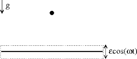
Figure 1: Schematic description of the model.

The dynamics of each individual particle, as usual in the literature [2], is described by a two-dimensional and nonlinear map for the variables velocity of the particle $V$ and time $t$ at each impact with the boundary. For a simplified gas model, the moving platform may be represented by a rigid wall or even the ground and the motion can be caused by the atomic oscillations at the edge of the wall. Because such atomic oscillations are too small [37] as compared to the positions or displacements made by each particle, we can approximate the description by assuming the time of flight of each particle is calculated as if the wall was fixed. However, the exchange of energy is determined by a moving wall. This approach is reasonable because the atomic oscillations are from the order of $10^{-11}m$ (see [37]). Under this assumption, the mapping is written as

$$\left\{\begin{array}[]{ll}t_{n+1}=\left[t_{n}+2{{V_{n}}\over{g}}\right]~{}{\rm mod~{}(2\pi/\omega)}\\ V_{n+1}=|\gamma V_{n}-(1+\gamma)\epsilon\omega\sin(\omega t_{n+1})|\end{array}\right..$$ (2)

The modulus used in the second equation is introduced to avoid a specific situation. After the collisions, there could be a small possibility of the particle present a negative velocity. This case has no physical meaning in the model because the wall is assumed to be fixed in order to make easier the calculation of the time of flights. Then a particle moving with a negative velocity after the collision is forbidden. If such a case happens, the particle is injected back to the dynamics with the same velocity but with a positive direction. The parameter $\gamma$ denotes the restitution coefficient for the impacts. Indeed $\gamma\in[0,1]$. As we will see, for $\gamma=1$ the conservative dynamics is observed. For a specific range of control parameters, this leads to an unlimited diffusion in velocity [29] therefore characterising a phenomenon called as Fermi acceleration [31]. As a physical interpretation from a thermodynamical point of view, it would leads to an infinite temperature of a classical gas. This is quite contradictory to what is observed in real experiments or in day life. On the other hand when inelastic collisions are taken into account, the unlimited diffusion of the velocity of the ensemble of particles is suppressed, leading to a finite temperature most in agreement to what is confirmed in experiments. We discuss both cases separately.

2.1 Conservative dynamics

Let us discuss in this section the behaviour of the average velocity for an ensemble of particles for the restitution coefficient $\gamma=1$. Under this condition, the mapping simplifies to

$$\left\{\begin{array}[]{ll}t_{n+1}=\left[t_{n}+2{{V_{n}}\over{g}}\right]~{}{\rm mod~{}(2\pi/\omega)}\\ V_{n+1}=|V_{n}-2\epsilon\omega\sin(\omega t_{n+1})|\end{array}\right..$$ (3)

The expression for mapping (3) is remarkably similar to the one describing the standard map [2] (please see appendix 1). There are few steps we have to proceed to make a connection between the two models: (1) multiply first equation of map (3) by $\omega$; (2) multiply the second equation of map (3) by $2\omega/g$; (3) define both $\tilde{\phi}=\omega t$ and $I=2\omega V/g$; (4) define $\phi_{n+1}=\tilde{\phi}_{n}+\pi$. After these steps, we obtain an effective control parameter as

$$K_{\rm eff}={{4\epsilon\omega}\over{g}}~{}.$$ (4)

Therefore for $K_{\rm eff}>K_{c}$ the phase space allows to unlimited diffusion in the velocity [29]. To make sure we are considering such case, in our numerical simulations we shall consider only

$${{\epsilon\omega}\over{g}}\geq 0.2429\ldots~{}.$$ (5)

To give an analytical argument on the unlimited diffusion, let us start the ensemble of particles with a low initial velocity. We mean low here an ensemble with low temperature but large enough so that quantum effects can be disregarded. Then squaring second equation of mapping (3) we obtain

$$V_{n+1}^{2}=V_{n}^{2}-4\epsilon\omega V_{n}\sin(\omega t_{n+1})+4\epsilon^{2}\omega^{2}\sin^{2}(\omega t_{n+1})~{}.$$ (6)

Taking an average over an ensemble of different initial times $t\in[0,2\pi/\omega]$, we end up with

$$\overline{V^{2}}_{n+1}-\overline{V^{2}}_{n} = {{\overline{V^{2}}_{n+1}-\overline{V^{2}}_{n}}\over{(n+1)-n}}~{},$$ (7)

$$\cong {{\partial\overline{V^{2}}}\over{\partial n}}=2\epsilon^{2}\omega^{2}~{}.$$

We have then a differential equation involving $\overline{V^{2}}$ and $n$. Doing the integration properly we obtain that

$$V_{\rm rms} = \sqrt{\overline{V^{2}}}~{},$$ (8)

$$= \sqrt{V_{0}^{2}+2\epsilon^{2}\omega^{2}n}~{}.$$

For a low initial velocity $V_{0}\rightarrow 0$ then we see $V_{\rm rms}\propto n^{{1}\over{2}}$. Figure 2 shows a plot of the numerical simulation made for an ensemble of $5,000$ different initial conditions at the same initial velocity. The slope of growth is $1/2$ as theoretically given by Eq. (8).

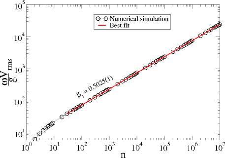
Figure 2: Plot of the average velocity as a function of $n$. A power law fitting furnishes a slope of $0.5025(1)\cong 1/2$, in remarkably well agreement with Eq. (8). The parameters used were such that $(\epsilon\omega^{2}/g)=10$.

The result presented in Fig. 2 confirms the unlimited growth of the average velocity, leading to the phenomenon of Fermi acceleration. However, it is in disagreement with experimental results because a temperature in a room can not grow unbound. In next section we consider the dynamics under the effects of inelastic collisions.

2.2 Dissipative dynamics

Let us discuss here the implications of the inelastic collisions in the steady state dynamics. According to the theory of dynamical systems [6], the presence of dissipation in the system may lead to the existence of attractors in the system. The determinant of the Jacobian matrix of mapping (1) is $\gamma~{}\rm{sign}[\gamma V_{n}-(1+\gamma)\epsilon\omega\sin(\omega t_{n+1})]$ where $\rm{sign}(u)=1$ for $u>0$ and $\rm{sign}(u)=-1$ for $u<0$. This is indeed a quite strong mathematical result. According to Liouville’s theorem [38], area contraction in the phase space is happening, therefore for any $\gamma<1$ attractors must exist in the phase space. Given they are far away from the infinity, unlimited diffusion must not be observed anymore. Our results corroborate with this. Moreover if the dissipation suppresses the unlimited diffusion in velocity, Fermi acceleration is suppressed too making us to reinforce that it is not a robust phenomena [39].

To make some theoretical progress, we start squaring the second equation of mapping (2), that leads to

$$V^{2}_{n+1}=\gamma^{2}V^{2}_{n}-2\gamma V_{n}(1+\gamma)\epsilon\omega\sin(\omega t_{n+1})+(1+\gamma)^{2}\epsilon^{2}\omega^{2}\sin^{2}(\omega t_{n+1})~{}.$$ (9)

Doing an ensemble average for $t\in[0,2\pi/\omega]$ and grouping properly the terms we obtain

$$\overline{V^{2}}_{n+1}=\gamma^{2}\overline{V^{2}}_{n}+{{(1+\gamma)^{2}\epsilon^{2}\omega^{2}}\over{2}}~{}.$$ (10)

Equation (10) can be used in different forms. We start with considering the stationary state.

2.2.1 Stationary state

For the stationary state, we have that $\overline{V^{2}}_{n+1}=\overline{V^{2}}_{n}=\overline{V^{2}}$. Substituting this result in Eq. (10) we end up with an expression of the type

$$\overline{V^{2}}={{(1+\gamma)}\over{2}}{{\epsilon^{2}\omega^{2}}\over{(1-\gamma)}}~{},$$ (11)

and that when applying square root from both sides

$$V_{\rm rms}={\sqrt{{(1+\gamma)}\over{{2}}}}{{\epsilon\omega}\over{(1-\gamma)^{{}^{1}/_{2}}}}~{}.$$ (12)

Notice that the steady state velocity does indeed depends on two terms: (i) from the product of $\epsilon\omega$, which corresponds to the maximum velocity of the moving wall, i.e., maximum atomic speed in the wall and; (ii) on the inverse of the square root of the dissipation, namely $(1-\gamma)^{-1/2}$.

2.2.2 Evolution to the stationary state

Let us discuss here how does the average velocity of the ensemble goes to the equilibrium. If the initial velocity given for the ensemble is lower than the one expressed by Eq. (12), then we should observe a regime of growth until reaching the stationary state. One the other hand if is large enough, there must be observed a decrease on the velocity until stationary state is reached. As we will see, the two regimes approach the equilibrium in different ways. We shall show the growth of the average velocity is given by a power law while the decay of energy is remarkably fast given by an exponential function.

To have a glance on this we consider equation (11) rewritten in a convenient way as

$$\overline{V^{2}}_{n+1}-\overline{V^{2}}_{n} =\Delta V^{2} ={{\overline{V^{2}}_{n+1}-\overline{V^{2}}_{n}}\over{(n+1)-n}}\cong{{\partial\overline{V^{2}}}\over{\partial n}}~{},$$ (13)

$$= \overline{V^{2}}(\gamma^{2}-1)+{{(1+\gamma)^{2}\epsilon^{2}\omega^{2}}\over{2}}~{}.$$

Proceeding with the integration and after grouping the terms properly we obtain

$$\overline{V^{2}}(n)=V_{0}^{2}e^{(\gamma^{2}-1)n}+{{(1+\gamma)\epsilon^{2}\omega^{2}}\over{2(1-\gamma)}}\left[1-e^{(\gamma^{2}-1)n}\right]~{}.$$ (14)

We see from Eq. (14), and as expected, an explicit dependence on the initial velocity, which allows us to make to distinct investigations: (1) consider the case of $V_{0}\gg\epsilon\omega$ and; (ii) the case of $V_{0}\ll\epsilon\omega$. We start with (i) first.

For the case of $V_{0}\gg\epsilon\omega$, the first term of Eq. (14) dominates over the second one. Taking square root of both sides leads to

$$V_{\rm rms}(n)=V_{0}e^{{(\gamma^{2}-1)n}\over{2}}~{}.$$ (15)

The numerator heading the exponential can be factored and considering the case of low dissipation, i.e. $\gamma\cong 1$ which gives $(1+\gamma)\cong 2$, therefore we obtain that

$$V_{\rm rms}(n)=V_{0}e^{(\gamma-1)n}~{},$$ (16)

which is an exponential function as we mention before. Figure 3

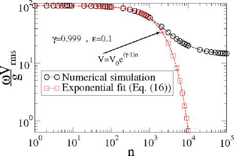
Figure 3: Decay of the average velocity as function of $n$. Circles denote the numerical simulation while squares correspond to the exponential fit given by Eq. (16).

shows the behaviour of the decay of the average velocity for the control parameter $\gamma=0.999$ and $(\epsilon\omega^{2}/g)=0.1$, which was chosen to make the second term slower and being possible to observe the decay in a convenient way. We see the two curves, one marked by circles, produced by numerical simulation, agree with the theoretical result given by Eq. (16) and plotted as squares, for short $n$. As soon as $n$ grows and the second term in Eq. (14) becomes considerable, the curves split from each other.

The exponential decay can be determined also from a different way. Indeed it emerges naturally from iteration of the mapping. From the second equation of mapping (2) we obtain $V_{1}=\gamma V_{0}$. If we iterate again we have $V_{2}=\gamma V_{1}=\gamma^{2}V_{0}$. For $V_{3}=\gamma V_{2}=\gamma^{3}V_{0}$. Finally after $n$ iterations we obtain

$$V_{n}=\gamma^{n}V_{0}~{}.$$ (17)

We can then expand Eq. (17) in Taylor series and obtain

$$V_{n} = V_{0}\left[1+(\gamma-1)n+{{1}\over{2}}(\gamma-1)^{2}n(n-1)+{{1}\over{6}}(\gamma-1)^{3}n(n-1)(n-2)\right]+$$ (18)

$$+ V_{0}\left[{{1}\over{24}}(\gamma-1)^{4}n(n-1)(n-2)(n-3)+\ldots\right]~{}.$$

For $n\gg 1$, we can rewrite Eq. (18) as

$$V_{n}=V_{0}\left[1+(\gamma-1)n+{{1}\over{2}}(\gamma-1)^{2}n^{2}+{{1}\over{6}}(\gamma-1)^{3}n^{3}+{{1}\over{24}}(\gamma-1)^{4}n^{4}+\ldots\right]~{},$$ (19)

which is the own definition of the exponential given by Eq. (16).

For the case of $V_{0}\ll\epsilon\omega$, the average velocity grows and eventually bends towards a regime of saturation, which is marked by a constant plateau for long enough $n$, as can be seen from Fig. 4.

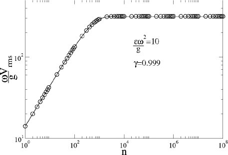
Figure 4: Plot of the average velocity as function of $n$ for the case of $V_{0}\ll\epsilon\omega$.

The curve shown in Fig. 4 grows with $n^{1/2}$ and, after reaching a typical number of collisions marking a crossover, it bends in direction of the stationary state. The behaviour shown in Fig. 4 has many more important properties which we address in the next section, in particular a scaling behaviour.

3 Numerical results and scaling properties

In this section we discuss with more details the behaviour observed in Fig. 4. It is however more convenient to do numerical simulations if we define a set of dimensionless variables. We then define

$$v={{\omega V}\over{g}}~{}~{}~{},~{}~{}~{}\phi=\omega t~{}~{}~{},~{}~{}~{}\varepsilon={{\epsilon\omega^{2}}\over{g}}~{},$$ (20)

where the parameter $\varepsilon$ corresponds to the ratio of the maximum acceleration of the wall by the acceleration of the gravity. In this new set of variables the map is written as

$$\left\{\begin{array}[]{ll}\phi_{n+1}=[\phi_{n}+2v_{n}]~{}{\rm mod~{}(2\pi)}\\ v_{n+1}=|\gamma v_{n}-(1+\gamma)\varepsilon\sin(\phi_{n+1})|\end{array}\right..$$ (21)

Let us give a short discussion on the most relevant control parameter of the three originally involved. Indeed we assume the gravitational field $g$ is constant. Because of the constraints of the wall as a solid body, the amplitude of oscillation can not change much. Therefore the most significant control parameter to the dynamics is the angular frequency $\omega$. Moreover it appears as a power of $2$ in the definition of $\varepsilon$. Since the atomic oscillation is really high [40], say from the order of $10^{13}Hz$, a small modification on $\omega$ causes large variation on $\varepsilon$.

Before discuss the behaviour of the average velocity as a function of the control parameters, let us check if the theoretical result obtained from Eq. (14) is in well agreement with the numerical simulations. It is shown in Fig. 5 a plot of the the dimensionless average velocity as a function of $n$ for both the simulation (circles) and theoretical (squares).

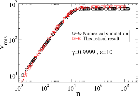
Figure 5: Plot of the dimensionless average velocity as function of $n$ for the case of $V_{0}\ll\epsilon\omega$ and considering: simulation (circles) and theoretical given by Eq. (14) (square).

We can see from the two curves a remarkable agreement, therefore letting us to proceed with the theoretical investigation.

The behaviour of the average velocity plotted against $n$ for different control parameters is shown in Fig. 6(a).

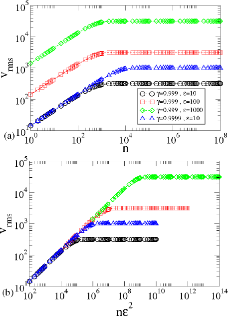
Figure 6: (a) Plot of the dimensionless average velocity as function of $n$ for the case of $V_{0}\ll\epsilon\omega$ and considering different control parameters, as labelled in the figures. (b) Same plot of (a) after a transformation $n\rightarrow n\varepsilon^{2}$.

We see the curves of the average velocity start to grow with for short $n$ and, after reaching a crossover collision number $n_{x}$, they bend towards a regime of saturation. Different control parameters lead the curves to saturate at different values. The crossover $n_{x}$ does not seem to depend on the parameter $\varepsilon$, as we shall confirm latter. However it does indeed depends on the parameter $\gamma$. It is convenient to apply a transformation $n\rightarrow n\varepsilon^{2}$ that makes all curves start grow together as can be seen in Fig. 6(b). This transformation also makes the horizontal axis to have the same dimension as given by Eq. (8).

The behaviour shown in Fig. 6 makes us to propose the following scaling hypotheses:

1. $$\overline{v}\propto(n\varepsilon^{2})^{\beta}~{},{\rm~{}for~{}n\ll n_{x}}~{},$$ (22)

   where $\beta$ is called as the acceleration exponent;

2. $$\overline{v}_{\rm sat}\propto\varepsilon^{\alpha_{1}}(1-\gamma)^{\alpha_{2}}~{},~{}{\rm~{}for~{}n\gg n_{x}}~{},$$ (23)

   where $\alpha_{1}$ and $\alpha_{2}$ are the saturation exponents;

3. $$n_{x}\propto\varepsilon^{z_{1}}(1-\gamma)^{z_{2}}~{},$$ (24)

   where $z_{1}$ and $z_{2}$ are the crossover exponents.

The five exponents $\beta$, $\alpha_{1}$, $\alpha_{2}$, $z_{1}$ and $z_{2}$ are called as critical exponents.

The three scaling hypotheses shown in Eqs. (22), (23) and (24) allow us to describe the behaviour of the average velocity in terms of a homogeneous generalised function of the type

$$\overline{v}(n\varepsilon^{2},\varepsilon,(1-\gamma))=\ell\overline{v}(\ell^{a}n\varepsilon^{2},\ell^{b}\varepsilon,\ell^{c}(1-\gamma))~{},$$ (25)

where $\ell$ is a scaling factor, $a$, $b$ and $c$ are characteristic exponents and are related to the critical exponents.

Choosing $\ell^{a}n\varepsilon^{2}=1$ we obtain

$$\ell=(n\varepsilon^{2})^{{}^{-1}/_{a}}~{}.$$ (26)

Substituting this result in Eq. (25) we have

$$\overline{v}=(n\varepsilon^{2})^{{}^{-1}/_{a}}\overline{v_{1}}((n\varepsilon^{2})^{{}^{-b}/_{a}}\varepsilon,(n\varepsilon^{2})^{{}^{-c}/_{a}}(1-\gamma))~{},$$ (27)

where the function $\overline{v_{1}}$ is assumed to be constant for $n\ll n_{x}$. Comparing the result given by Eq. (27) with the first scaling hypotheses given by Eq. (22), we obtain that $\beta=-1/a$. The exponent $\beta$ was indeed confirmed as $\beta=1/2$, then $a=-2$.

Considering now $\ell^{b}\varepsilon=1$ we have

$$\ell=\varepsilon^{{}^{-1}/_{b}}~{}.$$ (28)

Substituting again this result in Eq. (25) we find

$$\overline{v}=\varepsilon^{{}^{-1}/_{b}}\overline{v_{2}}(\varepsilon^{{}^{-a}/_{b}}(n\varepsilon^{2}),\varepsilon^{{}^{-c}/_{b}}(1-\gamma))~{},$$ (29)

where the function $\overline{v_{2}}$ is again assumed to be constant for $n\gg n_{x}$. Comparing Eq. (29) with the second scaling hypotheses given by Eq. (23) we obtain that $\alpha_{1}=-1/b$. We have already a theoretical result for the exponent $\alpha_{1}$, which must be checked with numerical simulation latter, as we will do. But a comparison with Eq. (12) yields that $\alpha_{1}=1$. Then scaling exponent $b=-1$.

Considering now $\ell^{c}(1-\gamma)=1$, we have

$$\ell=(1-\gamma)^{{}^{-1}/_{c}}~{}.$$ (30)

Substituting again the result obtained from Eq. (30) in Eq. (25) we obtain

$$\overline{v}=(1-\gamma)^{{}^{-1}/_{c}}\overline{v_{3}}((1-\gamma)^{{}^{-a}/_{c}}(n\varepsilon^{2}),(1-\gamma)^{{}^{-b}/_{c}}\varepsilon)~{},$$ (31)

where the function $\overline{v_{3}}$ is assumed constant for $n\gg n_{x}$. Comparing this result with second scaling hypotheses given by Eq. (23), we obtain $\alpha_{2}=-1/c$. Theoretical result for critical exponent $\alpha_{2}$ also comes from Eq. (12) and yields $\alpha_{2}=-1/2$. Therefore the scaling exponent $c=2$.

The next step is to relate the critical exponents among themselves and obtain the scaling laws. To do that, we compare the different expressions obtained for $\ell$. First comparison is made between Eqs. (26) and (28) and that leads to

$$n=\varepsilon^{{{\alpha_{1}}\over{\beta}}-2}~{}.$$ (32)

Equation above can be compared with third scaling hypotheses given by Eq. (24), and that gives us

$$z_{1}={{\alpha_{1}}\over{\beta}}-2~{}.$$ (33)

Comparing now the expressions for $\ell$ given by Eqs. (26) and (30) and assuming that $\varepsilon$ is constant we obtain

$$n=(1-\gamma)^{{\alpha_{2}}\over{\beta}}~{},$$ (34)

and hence comparing with the third scaling hypotheses given by Eq. (24) gives

$$z_{2}={{\alpha_{2}}\over{\beta}}~{}.$$ (35)

The theoretical values for the critical exponents $\alpha_{1}$ and $\alpha_{2}$ are given by Eq. (12). They are indeed well confirmed from numerical simulations, as shown in Fig. 7.

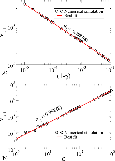
Figure 7: (a) Plot of $v_{\rm sat}$ as a function of $(1-\gamma)$. A power law fitting gives $\alpha_{2}=-0.4987(8)\cong-1/2$. (b) Plot of $v_{\rm sat}$ as a function of $\varepsilon$. A power law fitting furnishes $\alpha_{1}=0.998(8)\cong 1$.

Since the exponents $\beta$, $\alpha_{1}$ and $\alpha_{2}$ are known, the two scaling laws given by Eqs. (33) and (35) can be evaluated to obtain $z_{1}$ and $z_{2}$. When we substitute the numerical values for $\beta=1/2$, $\alpha_{1}=1$ and $\alpha_{2}=-2$ we obtain that $z_{1}=0$ and $z_{2}=-1$. The result $z_{1}=0$ is not a surprise. Indeed if we look at Fig. 6(a) we see that the crossover $n_{x}$ is the same and is independent on $\varepsilon$, but do indeed depend on $\gamma$. The exponent $z_{2}=-1$ can also be confirmed by numerical simulation. Figure 8 shows a plot of the crossover $n_{x}$ as a function of $(1-\gamma)$. The slope obtained is $z_{2}=-0.998(2)\cong-1$ in a remarkably well agreement with the theoretical prediction.

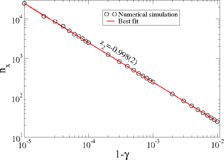
Figure 8: Plot of the crossover $n_{x}$ as a function of $(1-\gamma)$. A power law fitting furnishes $z_{2}=-0.998(2)$ in well agreement with the result of Eq. (35).

The exponents $z_{1}$ and $z_{2}$ can also be obtained from theoretical analysis. Indeed if we equalling the equation describing the growth of the velocity, Eq. (8) with the equation given the stationary state, Eq. (12), both in dimensionless variables, the isolated $n$ gives the crossover as function of either $\varepsilon$ and $\gamma$. Then we obtain

$$\sqrt{v^{2}_{0}+2n\varepsilon^{2}}={\sqrt{{(1+\gamma)}\over{{2}}}}{{\varepsilon}\over{(1-\gamma)^{{1}\over{2}}}}~{},$$ (36)

and when considering the initial velocity sufficiently small, i.e. $v_{0}\cong 0$, we end up with

$$n_{x}={{(1+\gamma)}\over{4}}(1-\gamma)^{-1}~{}.$$ (37)

The result given by Eq. (37) confirms two things: (i) that the exponent $z_{2}=-1$, as obtained by the scaling law (35) and confirmed by numerical simulation from Fig. 8 and; (ii) that the crossover is independent on $\varepsilon$, leading to $z_{1}=0$ and as mentioned before.

Other property emerging from the critical exponents is the scaling invariance of the curves shown in Fig. 6. If the axis of Fig. 6(a) are rescaled according to these two transformations namely

$$v \rightarrow {{v}\over{\varepsilon^{\alpha_{1}}(1-\gamma)^{\alpha_{2}}}}~{},$$ (38)

$$n \rightarrow {{n}\over{(1-\gamma)^{z_{2}}}}~{},$$ (39)

all the curves are merged onto a single and universal plot, as shown in Fig. 9.

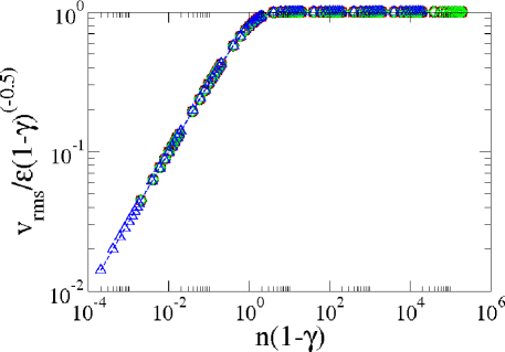
Figure 9: Overlap of all curves shown in Fig. 6(a) onto a single and universal plot, after the application of the transformations given by Eqs. (38) and (39).

4 Relation between number of collisions and time

In this section we discuss a way on how to relate the number of collisions and time. Indeed, from an experimental point of view, measuring the number of collisions of particles almost massless would be a very difficult task. Instead of measuring the number of collisions, the easiest parameter is the time. The main goal of this section is then to relate $n$ and time $t$.

Starting with an experiment, the time can be obtained from

$$t=\Delta t_{c1}+\Delta t_{c2}+\Delta t_{c3}+\ldots+\Delta t_{cn}~{},$$ (40)

where $\Delta t_{ci}$ with $i=1,2,3,\ldots,n$ gives the interval of time between two collisions of the same particle. It then gives us an expression of the type

$$t = {{2V_{0}}\over{g}}+{{2V_{1}}\over{g}}+{{2V_{2}}\over{g}}+\ldots+{{2V_{n}}\over{g}}~{},$$ (41)

$$= {{2}\over{g}}\sum_{i=0}^{n-1}~{}V_{i}.$$

If the number of collisions is relatively large, which in the majority of the situations is, we can approximate the sum of Eq. (41) by an integral of the type

$$t={{2}\over{g}}\int_{0}^{n}V(\tilde{n})d\tilde{n}~{}.$$ (42)

To make the integral we have to relate indeed $V$ directly with the number of collisions $n$. This seems to be a difficult task at first sigh. However, the behaviour shown in Fig. 9 can be described, and it indeed was with success [41], by an empirical function of the type

$$f(x)=\left[{{x}\over{1+x}}\right]^{\beta}~{},$$ (43)

where $f$ stands for the vertical axis, $x$ stands for the horizontal axis and $\beta$ is the accelerating exponent, which for our case here is $\beta=1/2$. Figure 10

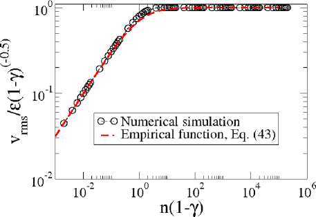
Figure 10: Overlap of a rescaled curve with the empirical function given by Eq. (43).

shows the two curves of rescaled velocity and empirical function given by Eq. (43). We see an astonishing agreement between the two. This is the link we need to relate velocity $v$ and number of collisions $n$.

With the empirical function at hands, we obtain that

$${{v}\over{\varepsilon^{\alpha_{1}}(1-\gamma)^{\alpha_{2}}}}=\left[{{\left({{n}\over{(1-\gamma)^{z_{2}}}}\right)}\over{\left(1+{{n}\over{(1-\gamma)^{z_{2}}}}\right)}}\right]^{\beta}~{}.$$ (44)

Considering the numerical values obtained for the critical exponents, namely $\alpha_{1}=1$, $\alpha_{2}=-1/2$, $z_{2}=-1$ e $\beta=1/2$, we can rewrite Eq. (44) as

$${{v}\over{\varepsilon}}\sqrt{1-\gamma}=\sqrt{{{n(1-\gamma)}\over{1+n(1-\gamma)}}}~{}.$$ (45)

Since the dimensionless variables were obtained from $v=\omega V/g$ and $\varepsilon=\epsilon\omega^{2}/g$, we can then return to the original variable $V$ and obtain

$$V(n)={{\epsilon\omega}\over{\sqrt{1-\gamma}}}\sqrt{{n(1-\gamma)}\over{1+n(1-\gamma)}}~{}.$$ (46)

The expression given by Eq. (46) can now be used to make the integration in Eq. (42). Then we have

$$t={{2}\over{g}}\int_{0}^{n}{{\epsilon\omega}\over{\sqrt{1-\gamma}}}\sqrt{{\tilde{n}(1-\gamma)}\over{1+\tilde{n}(1-\gamma)}}d\tilde{n}~{}.$$ (47)

Using $n^{\prime}=\tilde{n}(1-\gamma)$ and grouping the terms properly we end up with

$$t={{2\epsilon\omega}\over{g\sqrt{1-\gamma}(1-\gamma)}}\int_{0}^{n(1-\gamma)}\sqrt{{n^{\prime}}\over{1+n^{\prime}}}dn^{\prime}~{}.$$ (48)

After doing the integral we obtain

$$t = {{2\epsilon\omega}\over{g\sqrt{1-\gamma}(1-\gamma)}}\left[-{{1}\over{2}}\ln(n(1-\gamma))+\sqrt{n^{2}(1-\gamma)^{2}+n(1-\gamma)}\right]-$$ (49)

$$- {{2\epsilon\omega}\over{g\sqrt{1-\gamma}(1-\gamma)}}\ln\left(1+\sqrt{1+{{1}\over{n(1-\gamma)}}}\right)~{}.$$

For $n\gg 1$, there is only one dominant term in Eq. (49), that leads to

$$t \cong {{2\epsilon\omega}\over{g\sqrt{1-\gamma}(1-\gamma)}}[n(1-\gamma)]~{},$$ (50)

$$= {{2\epsilon\omega}\over{g\sqrt{1-\gamma}}}n~{}.$$

Isolating $n$ we have

$$n={{g\sqrt{1-\gamma}}\over{2\epsilon\omega}}t~{}.$$ (51)

Therefore this is the expression we need to obtain the observables as function of time instead of the number of collisions.

5 Connections with the thermodynamics

Let us discuss in this section the possible connections with the thermodynamics for the one-dimensional bouncer model. The first step is the discussion of the temperature. The connection of the squared velocity with the temperature comes from the energy equipartition theorem [42, 43]. Indeed, the theorem says that each quadratic term in the expression of the Hamiltonian (energy) of the system contributes with $K_{B}T/2$ in the thermal energy. Here $K_{B}$ stands for the Boltzmann constant. To apply the theorem, the system must be in equilibrium, i.e., reached the steady state. However, we want to describe the evolution of the temperature as function of both $n$ and time $t$, which may not be at equilibrium yet. We notice however there are basically two time scales involved in this problem. One of them is the time the particle spends travelling around (up and down) in between the collisions. This is a measurable time in the laboratory. The other one, which is several order of magnitude different, smaller indeed, is the period of an atomic oscillation, which is governed by the frequency of oscillation $\omega$. Then between one collision and the other, the atom has completed several thousands of billions of oscillations. Therefore between collisions, it can be considered that, from the scale of atomic oscillation, the velocity of the particle is almost constant, allowing to apply the theorem. In this way we have

$${{m\overline{V^{2}}}\over{2}}={{K_{B}T}\over{2}}~{},$$ (52)

yielding to

$$\overline{V^{2}}={{K_{B}T}\over{m}}~{}.$$ (53)

The four important expressions we have then in connection with the thermodynamics are the squared velocity and the temperature, both written as function of $n$ and time $t$, as given below. The first one is the squared velocity as function of $n$

$$\overline{V^{2}}(n)=V_{0}^{2}e^{(\gamma^{2}-1)n}+{{(1+\gamma)\epsilon^{2}\omega^{2}}\over{2(1-\gamma)}}\left[1-e^{(\gamma^{2}-1)n}\right]~{}.$$ (54)

The second is the temperature as function of $n$ too,

$$T(n)=T_{0}e^{(\gamma^{2}-1)n}+{{(1+\gamma)}\over{2}}{{m}\over{K_{B}}}{{\epsilon^{2}\omega^{2}}\over{(1-\gamma)}}[1-e^{(\gamma^{2}-1)n}]~{}.$$ (55)

The third and fourth are obtained from the Eqs. (54) and (55) but using the result given by Eq. (51). The squared velocity and temperature as a function of time are then written as

$$\overline{V^{2}}(t) = V_{0}^{2}e^{(\gamma^{2}-1){{g\sqrt{1-\gamma}}\over{2\epsilon\omega}}t}+{{(1+\gamma)\epsilon^{2}\omega^{2}}\over{2(1-\gamma)}}\left[1-e^{(\gamma^{2}-1){{g\sqrt{1-\gamma}}\over{2\epsilon\omega}}t}\right]~{},$$ (56)

$$T(t) = T_{0}e^{(\gamma^{2}-1){{g\sqrt{1-\gamma}}\over{2\epsilon\omega}}t}+{{(1+\gamma)}\over{2}}{{\epsilon^{2}\omega^{2}}\over{(1-\gamma)}}{{m}\over{K_{B}}}\left[1-e^{(\gamma^{2}-1){{g\sqrt{1-\gamma}}\over{2\epsilon\omega}}t}\right]~{}.$$ (57)

Other observable that can be obtained from the system is the entropy. Since we are considering the measure of the velocity of the particle at the instant of the collisions, the kinetic energy can then be written as

$$U(t)={{m}\over{2}}\overline{V^{2}}(t)={{K_{B}}\over{2}}T(t)~{}.$$ (58)

It is known [42] however that

$${{\partial S}\over{\partial U}}={{1}\over{T}}~{},$$ (59)

that yields to

$$dS={{1}\over{T}}dU~{},$$ (60)

where

$$T(t)={{2}\over{K_{B}}}U(t)~{}.$$ (61)

Then we obtain that

$$\int_{S_{0}}^{S}dS^{\prime}={{K_{B}}\over{2}}\int_{U_{0}}^{U}{{dU^{\prime}}\over{U^{\prime}}}~{}.$$ (62)

Doing the integral we have

$$S(t)=\tilde{S}+{{K_{B}}\over{2}}\ln(U(t))~{},$$ (63)

where $\tilde{S}$ is given by $\tilde{S}=S_{0}-K_{B}/2\ln(U_{0})$. Equation (63) can also be written in terms of the temperature, i.e.

$$S(t)=\tilde{S}+{{K_{B}}\over{2}}\ln\left[{{K_{B}}\over{2}}T(t)\right]~{}.$$ (64)

The result given by Eq. (63) shows the entropy is dependent on the energy and grows with the increase of the energy, which is already expected for an ideal gas [42, 43]. Either Eqs. (63) and (64) must be applied with some care, particularly in the domain of low energy, implying in low temperature. This is because at such regime, the entropy may assume negative values. Worst than that is that it can accelerate to $-\infty$ in the limit of $T\rightarrow 0$. Of course in such a limit our approach is not valid anymore and quantum description must be made.

6 Discussions

In this section we discuss our results obtained for the steady state regime. We see from Eq. (57) for long enough time, i.e., $t\rightarrow\infty$, we obtain

$$T(t\rightarrow\infty)={{(1+\gamma)}\over{2}}{{\epsilon^{2}\omega^{2}}\over{(1-\gamma)}}{{m}\over{K_{B}}}~{}.$$ (65)

The knowledge of the quantities $\epsilon$, $\omega$, $m$ and $T$ allow us to make an estimation of the restitution coefficient $\gamma$. Therefore isolating $\gamma$ from Eq. (65) we end up with

$$\gamma={{T(\infty)-{{\epsilon^{2}\omega^{2}m}\over{2K_{B}}}}\over{T(\infty)+{{\epsilon^{2}\omega^{2}m}\over{2K_{B}}}}}~{}.$$ (66)

To make an estimation of $\gamma$ we shall consider a light molecule, Hydrogen ($H_{2}$) indeed whose atomic mass is $m=2u_{a}$ where $u_{a}=1.660538921\times 10^{-27}kg$. We suppose also the molecule is colliding with a copper wall at room temperature $T=300K$. From Ref. [40], the frequency of oscillation is $\omega=4.49\times 10^{13}Hz$. The amplitude of oscillation comes from Ref. [37], but we must give a short discussion first.

According to the theoretical models of lattices, a cubic lattice is formed by atoms placed on each corner of a cube and also with an atom at each face of the cube. Then the lattice spacing describes the distance between two adjacent corners of the cube. By knowing the lattice spacing we make the following assumption. An atom can not vibrate freely. Due to the bonds with other atoms, it must vibrate only around its equilibrium position. We assume for doing the estimation of $\gamma$ that each atom oscillates with at most 5 percent of the lattice spacing (which may still be much). Then according to [37], $d_{l}=1.41\times 10^{-10}m$, yielding in $\epsilon=5d_{l}/100$.

With the numerical values of the parameters at hand, we evaluate Eq. (66) and found a naive estimation for the restitution coefficient of $\gamma\cong 0.92$.

Using this result to be applied in Eq. (56) yields a velocity of $V_{\rm rms}\cong 310m/s$. The model presented in this paper then succeeded well to argue on the suppression of Fermi acceleration and making a temperature finite in a gas. It may also present some applicability to estimate the restitution coefficient, what should be tested experimentally. However, it fails to estimate with good accuracy the velocity of a Hydrogen molecule in a gas at room temperature. Our result furnishes $V_{\rm rms}\cong V_{B}/3$ of the velocity measured from a Hydrogen as an ideal gas at room temperature in 3-D space [44]. The sub index $B$ stands for Boltzmann velocity.

7 Conclusions

We have considered in this paper the dynamics of a one-dimensional bouncer model as an approximation to describe a gas of classical particles moving along an axis under the influence of gravity. As it is known in the literature [29], we confirmed that when a conservative case is considered, depending on the set of control parameters [2], unlimited diffusion is observed for the velocity of the particle, leading to a phenomenon of Fermi acceleration [31]. However, this unlimited diffusion is not what one may observe in a laboratory. Therefore, when inelastic collisions are taken into account, the unlimited diffusion was suppressed [39] and we have shown two different scenarios evolving towards the stationary state. For large initial velocity, we prove that decay of the particle is described by an exponential function with the speed of the decay depending on the amount of the dissipation, namely $|(1-\gamma)|$. For very low initial velocity, we have shown the average velocity grows until bends towards a regime of convergence, indicating the steady state was reached. The stationary state depends on the control parameters as $\epsilon(1-\gamma)^{-1/2}$. The crossover marking the change from growth to the saturation depends on the dissipation $(1-\gamma)^{-1}$ and is not dependent on $\epsilon$. A scaling law describing such behaviour was obtained.

The connection with the thermodynamics was made by using the equipartition theorem [42]. We found expressions for the temperature as well as squared velocity in variables $n$, denoting the number of collisions of the particles with the wall, and $t$, which is the time. The later was only possible to obtain because the scaled velocity was described by an empirical function [41] relating explicitly velocity $V$ and $n$, as requested by the procedure. The expression of $T(t)$ so far is more convenient from experimental point of view and can be measured directly in the laboratory. An expression for the entropy was also obtained. It has validity only for the regime of temperature sufficiently large in the sense quantum effects are negligible.

Finally a comparison of the results obtained from the model was made with data obtained from [37] and [40] considering standard vibrations of atoms as well as frequencies and amplitudes. Our result indicate a restitution coefficient for the Hydrogen of $\gamma\cong 0.92$ experiencing collisions with a cooper platform at room temperature. Therefore an experiment must be made as an attempt to confirm possibly the result obtained for $\gamma$. As discussed above, our model however fails to predict with accuracy the average velocity of a gas at room temperature since our result for 1-D model gives $V_{\rm rms}\cong V_{B}/3$, for the case considered in the discussion. Here $V_{B}$ is the Boltzmann velocity for a 3-D ideal gas.

8 Acknowledgements

EDL acknowledges support from CNPq, FUNDUNESP and FAPESP (2012/23688-5), Brazilian agencies. This research was supported by resources supplied by the Center for Scientific Computing (NCC/GridUNESP) of the São Paulo State University (UNESP). ALPL thanks CNPq for financial support and is also grateful for the kind hospitality of School of Mathematics of University of Bristol - UK for the time spent as PhD Sandwich supported by CAPES CsF - 0287-13-0 (Brazilian agency), which is also acknowledged.

Appendix 1 - Standard map

The standard mapping is written as

$$\left\{\begin{array}[]{ll}I_{n+1}=I_{n}+K\sin(\theta_{n})\\ \theta_{n+1}=[\theta_{n}+I_{n+1}]~{}{\rm mod~{}(2\pi)}\end{array}\right.,$$ (67)

where $K$ is a control parameter that controls two different types of transition: (1) Integrability with $K=0$ to non-integrability for $K\neq 0$ and; (2) Transition from local for $K<K_{c}=0.9716\ldots$ to globally chaotic behaviour $K\geq K_{c}$. A global chaotic behaviour means the invariant spanning curves separating the phase space in different portions are all destroyed letting the chaotic sea to diffuse unbounded.

References

- [1] G. M. Zaslavsky, Physics of chaos in Hamiltonian Systems, Imperial College Press, London (1998)
- [2] A. J. Lichtenberg, M. A. Lieberman, Regular and chaotic dynamics (Appl. Math. Sci.) 38, Springer Verlag, New York, (1992)
- [3] S. H. Strogatz, Nonlinear Dynamics And Chaos: With Applications To Physics, Biology, Chemistry, And Engineering, Westview Pres, Cambridge (2001)
- [4] J. A. C. Gallas, Structure of the parameter space of the Hénon map, Phys. Rev. Lett. 70 2714 (1983)
- [5] D. F. M. Oliveira, E. D. Leonel, Parameter space for a dissipative Fermi-Ulam model, New Journal of Physics, 13 123012 (2011)
- [6] R. C. Hilborn, Chaos and Nonlinear Dynamics: An Introduction for Scientists and Engineers, Oxford University Press, New York (1994)
- [7] E. Ott, Chaos in Dynamical Systems, Cambridge Univ. Press, New York (1997)
- [8] G. M. Zaslavsky, Hamiltonian chaos and fractional dynamics, Oxford University Press, New York (2008)
- [9] N. Chernov, R. Markarian, Chaotic Billiards, American Mathematical Society, Rhode Island (2006)
- [10] M. V. Berry, Regularity and chaos in classical mechanics, illustrated by three deformations of a circular billiard, European Journal of Physics, 2, 91 (1981)
- [11] L. A. Bunimovich, On the ergodic properties of nowhere dispersing billiards, Communications in Mathematical Physics, 65, 295 (1979)
- [12] H. Bailin, Elementary Symbolic Dynamics And Chaos In Dissipative Systems, World Scientific Publishing Co. Pte. Ltd. Singapore (1989)
- [13] U. Feudel, C. Grebogi, B. R. Hunt, J. A. Yorke, map with more than 100 coexisting low-period periodic attractors, Phys. Rev. E 54, 71 (1996)
- [14] D. F. Tavares, E. D. Leonel, A Simplified Fermi Accelerator Model Under Quadratic Frictional Force, Brazilian Journal of Physics, 38, 58 (2008)
- [15] D. F. M. Oliveira, M. Robnik, E. D. Leonel, Dynamical properties of a particle in a wave packet: Scaling invariance and boundary crisis, Chaos, Solitons & Fractals, 44, 883 (2011)
- [16] R. L. Devaney, A First Course In Chaotic Dynamical Systems: Theory And Experiment, Westview Press, Cambridge (1992)
- [17] G. A. Luna-Acosta, J. A. Méndez-Bermudez, F. M. Izrailev, Quantum-classical correspondence for local density of states and eigenfunctions of a chaotic periodic billiard, Physics Letters A, 274, 192 (2000)
- [18] E. D. Leonel, P. V. E. McClintock, A crisis in the dissipative Fermi accelerator model, J. Phys. A: Math. Gen., 38, L425 (2005)
- [19] L. E. Reichl, A modern course in Statistical Physics, Wiley-vhc Verlag, Weinheim, (2009)
- [20] A.-L. Barabási, H. E. Stanley, Fractal Concepts in Surface Growth, Cambridge University Press, Cambridge (1985)
- [21] A. M. Figueiredo Neto, S. R. A. Salinas, The Physics of Lyotropic Liquid Crystals: Phase Transitions and Structural Properties, Monographs on the Physics and Chemistry of Materials, Oxford University Press, New York (2005)
- [22] L. P. Kadanoff, Statistical Physics: Statics, Dynamics and Renormalization, World Scientific Publishing Co. Pte. Ltd., Singapore (2000)
- [23] E. D. Leonel, P. V. E. McClintock, J. K. L. da Silva, Fermi-Ulam accelerator model under scaling analysis, Physical Review Letters, 93, 014101 (2004)
- [24] D. G. Ladeira, J. K. L. da Silva, Scaling features of a breathing circular billiard, Journal of Physics A, 41, 365101 (2008)
- [25] W. D. McComb, Renormalization methods: a guide for beginners, Oxford University Press, Oxford (2004)
- [26] R. K. Patria, Statistical Mechanics, Elsevier (2008)
- [27] L. D. Pustylnikov, On Ulam’s problem, Theoretical and Mathematical Physics, 57, 1035 (1983)
- [28] André L. P. Livorati, T. Kroetz, C. P. Dettmann, I. L. Caldas, E. D. Leonel, Stickiness in a bouncer model: A slowing mechanism for Fermi acceleration, Phys. Rev. E, 86, 036203 (2012)
- [29] A. J. Lichtenberg, M. A. Lieberman, R. H. Cohen, Fermi acceleration revisited, Physica D, 1, 291 (1980)
- [30] A. Yu. Loskutov, A. B. Ryabov, L. G. Akinshin, Mechanism of Fermi acceleration in dispersing billiards with time-dependent boundaries, Journal of Experimental and Theoretical Physics, 89, 966 (1999)
- [31] E. Fermi, On the origin of the cosmic radiation, Physical Review, 75, 1169 (1949)
- [32] M. Scheel, R. Seemann, M. Brinkmann, M. Di Michel, A. Sheppard, B. Breidenbach, S. Herminghaus, Morphological clues of wet granular pile stability, Nature Materials, 7, 189 (2008)
- [33] M. K. Muller, S. Luding, T. Poschel, Force statistics and correlations in dense granular packings, Chemical Physics, 375, 600 (2010)
- [34] A. K. Dubey, A. Bodrova, S. Puri, N. Brilliantov, Phys. Rev. E, 87, 062202 (2013)
- [35] J. A. Carrillo, T. Poschel, C Saluena, J. Fluid. Mech., 597, 119 (2008)
- [36] A. Sack, M. Heckel, J. E. Kollmer, F. Zimber, T. Poschel, Phys. Rev. Lett., 111, 018001 (2013)
- [37] M. P. Marder, Condensed Matter Physics, John Wiley & Sons, New Jersey (2010)
- [38] G. J. Sussman, J. Wisdom, M. E. Mayer, Structure and Interpretation of Classical Mechanics, MIT Press, Cambridge (2001)
- [39] E. D. Leonel, Breaking down the Fermi acceleration with inelastic collisions, J. Phys. A: Math. Theor., 40, F1077 (2007)
- [40] P. Hofmann, Solid State Physics: An Introduction, WILEY-VHC Verlag, Weinheim (2008)
- [41] D. F. M. Oliveira, M. Robnik, E. D. Leonel, Statistical properties of a dissipative kicked system: Critical exponents and scaling invariance, Physics Letters A, 376, 723 (2012)
- [42] F. Reif, Fundamentals of Statistical and Thermal Physics, McGraw-Hill, New York (1965)
- [43] K. Huang, Statistical Mechanics, John Wiley & Sons, Inc. (1963)
- [44] S. J. Blundell, K. M Blundell, Concepts in Thermal Physics, Oxford University Press, Oxford (2006)