Short- and Long- Time Transport Structures in a Three Dimensional Time Dependent Flow

Abstract

Lagrangian transport structures for three-dimensional and time-dependent fluid flows are of great interest in numerous applications, particularly for geophysical or oceanic flows. In such flows, chaotic transport and mixing can play important environmental and ecological roles, for examples in pollution spills or plankton migration. In such flows, where simulations or observations are typically available only over a short time, understanding the difference between short-time and long-time transport structures is critical. In this paper, we use a set of classical (i.e. Poincaré section, Lyapunov exponent) and alternative (i.e. finite time Lyapunov exponent, Lagrangian coherent structures) tools from dynamical systems theory that analyze chaotic transport both qualitatively and quantitatively. With this set of tools we are able to reveal, identify and highlight differences between short- and long-time transport structures inside a flow composed of a primary horizontal contra-rotating vortex chain, small lateral oscillations and a weak Ekman pumping. The difference is mainly the existence of regular or extremely slowly developing chaotic regions that are only present at short time.

I Introduction

Even if turbulence is not present in laminar flows, scalar transport in such systems can be very rich and complex. In particular, it is well known that in such systems, transport through successive mechanisms of stretching and folding of material lines in multiple directions may occur. For the past three decades, the kinematics viewpoint of fluid transport, i.e. the behavior of advected/passive particle trajectories, has received much attentionAref (2002). The generation of Lagrangian chaotic transport in a small Reynolds number flow is generally achieved by adding at least one degree of freedom to a two dimensional incompressible base flow. Such degrees of freedom often take the form of a weak time dependence Solomon and Gollub (1988b, a); Paoletti et al. (2006); Mancho et al. (2006) and/or weak dependence on the third dimension Bajer and Moffatt (1990); Kroujiline and Stone (1999).

The most general approach along these lines is to consider an incompressible three dimensional flow, the superposition of a two dimensional integrable flow ${\bm{V}}\left(x,y\right)$ and a small three dimensional unsteady perturbation $\epsilon_{0}{\bm{V}}\left(x,y,t\right)+\epsilon_{1}{\bm{V}}\left(x,y,z\right)$, $0\leq\epsilon_{0,1}\ll 1$. If the perturbed flow is unsteady and two-dimensional ($\epsilon_{0}\neq 0,\epsilon_{1}=0$), or steady and three-dimensional ($\epsilon_{0}=0,\epsilon_{1}\neq 0$), the kinematic behavior and Lagrangian transport structure are well known and established, with notably the existence of two-dimensional Kolmogorov Arnold Moser (KAM) tori acting as barrier to transport.

If the perturbed flow is composed of both an unsteady two dimensional and a steady three-dimensional perturbation ($\epsilon_{0}\neq 0,\epsilon_{1}\neq 0$), the situation is more complex with no theory still completely established yet. Depending on the number of fast (i.e. action) and slow (i.e. angle) variables that are necessary to described the system, the kinematic behavior, and consequently the Lagrangian transport structure, can be very different.

On the one hand, in flows described by one slow and two fast variables, action-angle-angle flows, the kinematic and Lagrangian space structure is similar to the simpler case (i.e. unsteady two dimensional or steady three-dimensional) with the presence of KAM-like regular tori acting as an impermeable barrier to transport. On the other hand, in action-action-angle flows, Arnold-like diffusion may appear, enabling essentially complete mixing via resonance phenomena.

These action-action-angle flows have an important place in the studies of Lagrangian transport. Indeed, such flows arise frequently in small (e.g. microfluidic devices) and large (e.g. geophysical or oceanic flows) scales where geometric symmetries severely constrain the flow structure, leading to the apparition of multiple flow actions.

While many previous works have focus on describing, both qualitatively Cartwright et al. (1996); Feingold et al. (1988); Piro and Feingold (1988); Cartwright et al. (1995) and quantitatively Vainchtein et al. (2006, 2007); Neishtadt (2005); Vainchtein et al. (2008), the long-time transport structure of these perturbed action-action-angle flows, we turn our attention to the short-time behavior. One motivation is that studying the long-time behavior of the system requires knowing or modeling the system over long times, which is not always possible or physically realistic. For example in oceanic flows simulations or observations are typically available only during a short time. Specifically, we seek to characterize and identify the transport structures present at short time with the help of alternative tools.

This paper is organized as follows. The physical model, as well as its assumptions and corresponding dynamical system, are first described. Then the different transport characteristics possible in this system are summarized. The Lagrangian structures at long time via Poincaré sections and infinite time Lyapunov exponent maps are shown. Finally, we present both qualitatively and quantitatively, the evidence of hidden transport structures present only at short time. Then these short time transport structures are revealed and clearly identified as Lagrangian coherent structures.

II Toy model

II.1 Apparatus

We consider the same magneto-hydrodynamic (MHD) flow system as Solomon and Gollub (see Fig. 1). An electric current passes through a thin layer of an electrolytic solution (salt water or dilute $H_{2}S0_{4}$) contained in a rectangular channel. The current interacts with the magnetic field produced by a series of magnets of alternating polarity embedded into the bottom wall, resulting in a periodic array of vortices separated by separatrices directly above the centers of the magnets. Time-dependent forcing is introduced in the system by displacing the fluid slowly back and forth across the magnets with the use of a plunger. Typical frequencies of the forcing are around 0.050${\rm~{}Hz}$, corresponding to a period significantly longer than the viscous time scale (of the order of 4${\rm~{}Hz}$).

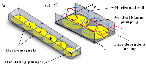
Figure 1: a) Sketch of the experimental device. A long channel characterized by a chain of electromagnets embedded into the floor with an oscillating plunger attached to one of the sides. b) Fluid flow: the base flow (blue) is a chain of alternating horizontal vortices; a weak perturbative flow (red) is generated naturally by Ekman pumping, which draws fluid inward along the bottom of the vortices and up the vortex centers.

II.2 Flow

Such an apparatus produces a flow composed of a primary horizontal alternating vortex chain (produced by the electromagnets), small lateral oscillations (created by the plunger) and a weak vertical secondary flow (generated by Ekman pumping). The features of the flow in Fig. 1, i.e. the crisscrossing of swirling rolls and time-dependent oscillations, are generic features in chaotic mixing problems and are present in many flows, notably in the ocean. A two-dimensional pair of contra-rotating swirling rolls is often used to model oceanic double gyres produced by the wind over the ocean’s surface Aharon et al. (2012); Samelson and Wiggins (2010); Samelson (1992); Liu and Yang (1994); Lekien and Coulliette (2007); Yan and Liu (1994), while the addition of a time dependent forcing and a vertical velocity can be justified to simulate wind variations or tidal effects and Ekman pumping present near fronts or induced by night convection Mahadevan and Tandon (2006). Critically, a simple analytical expression for the velocity field has been experimentally verified using a relatively easy to build small-scale apparatus.

II.3 Velocity field

We start from the Eulerian velocity field ${\bm{V}}=(u,v,w)$ and consider the particle path equations

$$u= \frac{dx}{dt} =-\cos(x+\epsilon_{0}\sin\omega t)\sin y+\epsilon_{1}\sin(2x+2\epsilon_{0}\sin\omega t)\sin z,$$ (1)

$$v= \frac{dy}{dt} =\sin(x+\epsilon_{0}\sin\omega t)\cos y+\epsilon_{1}\sin(2y)\sin z,$$ (2)

$$w= \frac{dz}{dt} =2\epsilon_{1}\cos z[\cos(2x+2\epsilon_{0}\sin\omega t)+\cos(2y)],$$ (3)

where $\omega$, $\epsilon_{0}$ and $\epsilon_{1}$ stand for the base oscillation’s frequency, its amplitude and the Ekman pumping strength, respectively.

The resulting velocity field and contour levels of the velocity magnitude in a generic cell for the three dimensional time-dependent case (i.e. $\epsilon_{0}\neq 0$ and $\epsilon_{1}\neq 0$) are represented in Fig. 2(a–c). Figures 2 illustrates how, inside a cell, the vortex pair is horizontally pushed forward and backward in time by the action of the plunger and how this two contra-rotating rolls structure is perturbed in third dimension by the vertical Ekman pumping.

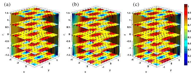
Figure 2: a–c) Velocity field and contour levels of the velocity intensity inside a generic cell for the three-dimensional time dependent case at time $t=\pi/2\omega,\pi\omega,3\pi/4\omega$.

III Time scales and transport characteristics as a function of parameters

III.1 Non-chaotic case

The steady two-dimensional case, corresponding to $\epsilon_{0,1}=0$, i.e. without periodic forcing and Ekman pumping, is characterized by two invariants (time-independent quantities), the stream function $\psi_{0}=\sin x\sin y~{}\in\left[-1,1\right]$ and the vertical position $z\in\left[-\pi/2,\pi/2\right]$. The streamlines of the non-chaotic case are curves of constant $\psi$ and $z$. The flow consists of a series of periodic cells, each cell consisting of two side-by-side recirculating rolls rotating in opposite directions as represented in Fig. 3. Within a generic cell, pathlines are organized into two sets of closed lines around a vertical line of degenerated elliptic fixed points, located at $\left(x=-\pi,y=0\right)$ and $\left(x=0,y=0\right)$. In addition, heteroclinic pathlines, connect degenerated hyperbolic fixed points located vertically on the corners of a generic half-cell, i.e. $\left(x=-3\pi/2,y=\pm\pi/2\right)$, $\left(x=-\pi,y=\pm\pi/2\right)$, $\left(x=\pi/2,y=\pm\pi/2\right)$ (see Fig. 3).
The frequency of motion on a streamline is given by

$$\frac{\pi}{\Omega(\psi)}=\int^{x_{max}}_{-\pi/2}\frac{dx}{\sqrt{\cos^{2}x-\psi^{2}}},$$

with $x_{max}=1/\cos\psi$ (see Ref. (Vainchtein et al., 2008) for more details). On every streamline we introduce a uniform phase $\chi\bmod 2\pi$ such that $\chi=0$ on the ${\bm{e}}_{x}-{\bm{e}}_{z}$ plane and $\dot{\chi}=\Omega\left(\psi\right)$. With this uniform phase, the non-chaotic flow can be described by using the variables $(\psi,z,\chi)$ instead of the Cartesian coordinates $(x,y,z)$, with

$$\dot{\psi} = 0,$$

$$\dot{z} = 0,$$

$$\dot{\chi} = \Omega(\psi).$$

Such a system is generally classified as action-action-angle, where the two invariants $\psi$ and $z$ are the two actions (constant quantities) and $\chi$ is the angle (oscillating quantity).

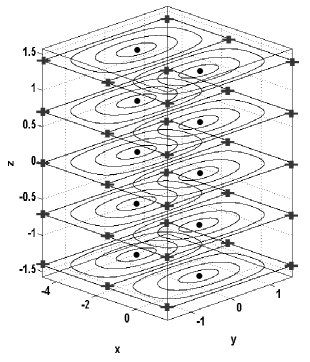
Figure 3: Streamlines in the integrable case $\epsilon_{0,1}=0$, degenerate elliptic points (bold points) and hyperbolic points (bold crosses).

III.2 Two-dimensional chaotic case

The slightly unsteady two-dimensional case, corresponding to $0<\epsilon_{0}\ll 1$ and $\epsilon_{1}=0$ is characterized by the evolution of a slow variable (perturbed action) and a fast variable (perturbed angle). The dynamical system expressed in the variables $(\psi,z,\chi)$ becomes

$$\dot{\psi} = \epsilon_{0}\sin\omega t~{}G_{0}\left(\psi,\chi\right),$$

$$\dot{z} = 0,$$

$$\dot{\chi} = \Omega(\psi)+\epsilon_{0}I_{0}\left(\psi,\chi\right),$$

where $G_{0}\left(\psi,\chi\right)=\sin 2y$ and $I_{0}$ is $2\pi$ periodic in $\chi$. The time perturbation enables the addition of a degree of freedom to the system, making the apparition of chaotic transport possible. In such perturbed cases, the phase space (real space in this case) dynamics is generally characterized by a mixed structure: a regular region in the center of the half-cells and a chaotic region around and between them, as shown in Fig. 4. Tracer particles within the vortices (localized around the position of the elliptic fixed points present in the non-chaotic case) remain confined there without being diffused to the other cells, while those in the chaotic sea (localized around the position of the heteroclinic orbits present in the steady case) diffuse to the other cells through chaotic transport. Such a structure is relatively simple and well understood with the Kolmogorov Kolmogorov (1954), Arnold Arnold (1963) and Moser Moser (1962) (K.A.M.) theory. Indeed, the KAM theorem precisely identifies which invariant quasi-periodic tori (acting as impermeable barriers to transport) are simply deformed and survive under the action of a weakly nonlinear perturbation from the tori which get destroyed and subsequently become chaotic.

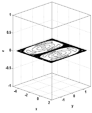
Figure 4: Poincaré section for the two-dimensional chaotic case with $\epsilon_{0}=0.10$, $\epsilon_{1}=0$ and $\omega=2.00$.

III.3 Three-dimensional chaotic case

The addition of even a small perturbation in the third dimension can make the structure of the flow much more complex. The number of slow variables and equivalently the number of time scales is crucial for the transport characteristics. When $0<\epsilon_{0,1}\ll 1$ one has an action-action-angle perturbed system, i.e. a system described by two slow variables and one fast variable:

$$\dot{\psi} = \epsilon_{0}\sin\omega t~{}G_{0}\left(\psi,\chi\right)-2\epsilon_{1}\sin z~{}\psi~{}G_{1}\left(\psi,\chi\right),$$

$$\dot{z} = 2\epsilon_{1}\cos z~{}H\left(\psi,\chi\right),$$

$$\dot{\chi} = \Omega(\psi)+\epsilon_{0}I_{0}\left(\psi,\chi\right)+\epsilon_{1}I_{1}\left(\psi,z,\chi\right),$$

where $H\left(\psi,\chi\right)=\cos 2y+\cos 2y$, $G_{1}\left(\psi,\chi\right)=\sin^{2}x+\sin^{2}y$ and $I_{1}$ is $2\pi$ periodic in $\chi$.

In such cases, behavior such as diffusion Cartwright et al. (1996); Feingold et al. (1988); Piro and Feingold (1988); Cartwright et al. (1995); Mezić (2001); Vainchtein et al. (2006, 2007, 2008) are present and may generate complete chaotic mixing at very long times, unlike action-angle-angle perturbed flows in which surviving KAM-like regular tori act as barrier to transport. In oceanography, understanding how the effect of a component in the third dimension, which is small and present only during a relatively short time, can influence the transport is of crucial importance. Consequently, we focus on the difference between short- and long-time transport structures in the weakly three-dimensional perturbed case, i.e. $0<\epsilon_{0}\ll\epsilon_{1}\ll 1$.

IV Long-time transport structures

IV.1 Qualitative observations

The classical approach in dynamical systems theory consists of studying the long time qualitative behavior of all possible trajectories. We do this first by using one of the most common tools, Poincaré sections. Figures 5 displays the double Poincaré sections (or Liouvillian sections, i.e. two-dimensional projections, using a combination of a stroboscopic map and a plane section) of the unsteady three dimensional flow (see Eqs. 1-3). Specifically, the Liouvillian sections considered here are the intersections of the trajectories at every period $2\pi/\omega$ with the planes $z=n\pi/6$, where $n=-2,-1,0,1,2$.
Each generic cell consists of a chaotic mixing region covering practically the whole space. At this long time (more than $1000$ periods have been computed) the trajectories seem to wander chaotically everywhere throughout the space without any apparent structure.

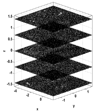
Figure 5: Horizontal double Poincaré sections (or Liouvillian sections) along the vertical axis for a single trajectory with parameter values $\epsilon_{0}=0.100$, $\epsilon_{1}=0.008$ and $\omega=2.000$.

IV.2 Quantitative observations

In order to gain further insight into the long-time transport structures within the channel, we compute the Lyapunov exponents map. The technique consists of associating a Lyapunov exponent $\lambda$ with an initial condition ${\bm{X}}_{0}=(x_{0},y_{0},t=0)$.
First, we consider the time evolution of the Jacobian $J^{t}\left(x,y\right)$ given by the tangent flow and the matrix of variations ${\bm{\nabla}}\bm{V}_{{\bm{\lambda}}}$ as

$$\frac{dJ^{t}}{dt}={\bm{\nabla}}{\bm{V}_{{\bm{\lambda}}}}\left(x,y,t\right)J^{t},\\$$ (4)

where $J^{0}=I$ is the two-dimensional identity matrix. The Lyapunov map is then defined as

$$\lambda\left({\bm{X}}_{0}\right)=\lim_{\tau\to+\infty}\,\frac{1}{\tau}\ln\left|\gamma_{max}\left({\bm{X}}_{0}\right)\right|,$$ (5)

where $\gamma_{max}$ is the largest eigenvalue (in norm) of the Jacobian $J^{\tau}$.

The Lyapunov map ${\bm{X}}_{0}\rightarrow\lambda\left({\bm{X}}_{0}\right)$ allows us to distinguish between the initial conditions leading to the presence of regular (non-mixing) islands, i.e. regions associated with zero Lyapunov exponent values, and the initial conditions leading to chaotic mixing characterized by positive Lyapunov exponent value. The structures in phase space are then easily identified and the relative sizes of the regular (non-mixing) islands determined. This tool can be used to determine not only the phase space structures, but also quantify the degree of the mixing produced. A large Lyapunov exponent indicates strong stretching and folding, which is the archetypal mechanism of chaotic mixing. Due to the symmetry of the system, the domain of the Lyapunov exponent map reported below has been chosen as a periodic cell of the channel, i.e. $\left\{-3\pi/2<x<\pi/2,-\pi/2<y<\pi/2,-\pi/2<z<\pi/2\right\}$.

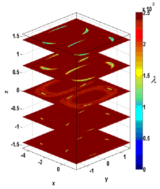
Figure 6: Lyapunov exponent field on the planes $z=n\pi/6$, with $n=-2,-1,0,1,2$.

Figure 6 shows horizontal sections of the Lyapunov field at long time for parameter values $\epsilon_{0}=0.10$, $\epsilon_{1}=0.08$ and $\omega=2.00$. It is clear that in Fig. 6, the chaotic transport is extremely well spread throughout the all cell space with a near-uniform distribution of the chaos intensity.

V Short-time transport structures

V.1 Short-time transport structure effects

V.1.1 Qualitative observations

First, we look at the transport behavior at short time by simply computing the time evolution of advected particles carried by the velocity field (see Eqs. 1-3). Figure 7 shows how two sets of advected particles, each initially concentrated at the center of the two half-cells, are transported during few hundreds of the forcing period $\omega$. It is clear that depending on the location inside the cell, particles seem to be transported either regularly or chaotically, in contrast with the widespread chaotic transport present at long time. The particles stay confined around the vertical axis and are regularly spread out near the top wall without displaying any sign of sensitivity to initial condition. However, near and along the vertical walls of the half-cell, the particles are heavily deformed by a mechanism of successive stretching and folding.

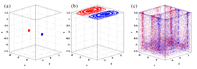
Figure 7: Dynamics of two sets of $100,000$ advected particles at time $t=0,150\pi/\omega,400\pi/\omega$ (a-c), for oscillation amplitude $\epsilon_{0}=0.100$, vertical flow strength $\epsilon_{1}=0.008$ and frequency $\omega=2.00$.

V.1.2 Quantitative observations

The results from Sec. IV seem in contradiction with those presented here, depicting Poincaré sections and Lyapunov field implying a well spread-out chaotic transport throughout the fluid domain (see Figs. 5-6). In order to gain more insight into this apparent contradiction, we have decided to quantify both the vertical and horizontal chaotic transport.

A good way to quantify the degree of mixing or chaotic transport as a function of spatial location is by determining the mixing index $M$ through the box counting method (see Ref. Stremler (2008)). This technique offers the advantage of being relatively easy to implement, fast and rather cheap in computing power. For this, we follow $N_{p}$ advected particles and divide the domain into $N_{x}\times N_{y}\times N_{z}$ boxes or cells. At each time, the number of particles $n_{i}$ is computed in each box, and from this the fraction of the total number of particles, or particle rate $r_{i}$. Given the number of particles $n_{i}$ inside each box $i$, the computation is performed as follows.

$$r_{i} = \frac{n_{i}}{n_{p}}~{}~{}\mbox{ if }n_{i}<n_{p},$$ (6)

$$r_{i} = 1~{}~{}~{}~{}~{}\mbox{ if }n_{i}\geq n_{p},$$

where $n_{p}$ is the average number of advected particles, i.e. $n_{p}=N_{p}/(N_{x}N_{y}N_{z})$. After computing the fraction of particles in each box and at each time $t$, the time evolution of the mixing index $M(t)$ is calculated by taking the average over all the boxes, i.e.

$$M(t)=\frac{1}{N_{x}N_{y}N_{z}}\sum_{i=1}^{N_{x}N_{y}N_{z}}r_{i}(t).$$

A mixing index converging towards zero ($\lim_{t\to+\infty}M(t)=0$) indicates an extremely weak mixing process, while a mixing index converging towards one ($\lim_{t\to+\infty}M(t)=1$) corresponds to a perfect mixing process.

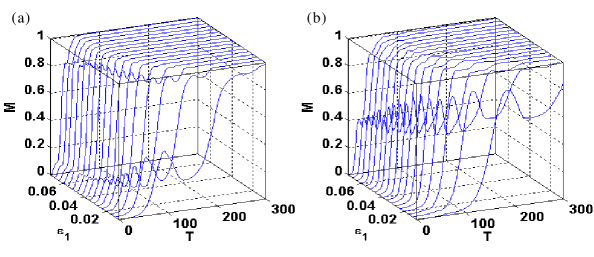
Figure 8: a) Horizontal ($N_{x}\times N_{y}\times N_{z}=3200\times 3200\times 1$) and b) vertical ($N_{x}\times N_{y}\times N_{z}=3200\times 1\times 3200$) mixing index as a function of the number of period $T=2\pi/\omega$ and vertical flow strength $\epsilon_{1}$ for $N_{p}=200,000$ advected particles.

Figures 8 illustrates the mixing index $M$ in the horizontal (i.e. $N_{x}\times N_{y}\times N_{z}=3200\times 3200\times 1$) and vertical (i.e. $N_{x}\times N_{y}\times N_{z}=3200\times 1\times 3200$) direction versus the time $t$ expressed in terms of the number of periods $T=2\pi/\omega$ and versus the vertical flow strength $\epsilon_{1}$.

The time evolution of $M$ both for the horizontal and vertical transport shows a very interesting behavior. $M$ starts from a very small value then increases in an oscillatory fashion (instead of increasing monotonously) to reach, at longer time, a plateau at $M=1$ indicating complete mixing. Such a behavior is in perfect accordance with the results seen up to here. The fact that the mixing index of both the vertical and horizontal mixing reaches at long time (i.e. $t>600\pi/\omega$) the limit $M=1$ corroborates the qualitative (Poincaré sections in Fig. 5) and quantitative (Lyapunov exponent field in Fig. 6) results showing that the long-time chaotic transport is complete. More importantly, the mixing index oscillations present at short times (representing alternations between horizontal and vertical chaotic transport) clearly reveal specific structures at short times. The effects of these short-time structure is qualitatively observed through the time evolution of dense sets of advected particles that are transported regularly near the horizontal walls and chaotically near the vertical walls.

Figure 8 shows also that as $\epsilon_{1}$ (i.e. the vertical flow strength) is increased, the amplitude of these oscillations diminish and vanish around $\epsilon_{1}\approx 0.1=\epsilon_{0}$. Such results, clearly indicate that this specific short-time structure is present only when the vertical flow is weak, i.e. $\epsilon_{1}<\epsilon_{0}$ and appears as some kind of remnant of the two-dimensional time dependent system $\epsilon_{1}=0$ (see Fig. 4).

Now that we have seen that the presence of a short time structure characterized by the combination of regular transport (around the vertical axis and near the horizontal walls) and chaotic transport (near the vertical walls of the half-cell), the next task is to reveal and identify these structures.

V.2 Identification of the short time transport structures

V.2.1 Short time Lyapunov exponent field

As stated in Sec. IV.2, the long time structures in phase space can easily be identified with the Lyapunov exponent field at infinite time. Using the same approach, the short time structure can be revealed with the Finite Time Lyapunov Exponent (FTLE) field.

Figure 9 shows FTLE map ${\bm{X}}_{0}\rightarrow\lambda\left({\bm{X}}_{0},\tau\right)$ on horizontal sections for time $\tau=\pm 20\pi/\omega$. FTLE maps for both positive and negative time have been computing to provide information about the forward and backward dynamics. In Fig. 9, we distinguish two regions: a region of weak chaotic transport (cold color) located around the vertical axis joining the two horizontal walls and a region of strong chaotic transport (hot color) near the vertical walls. Once again these results corroborate the existence of a short time structure transporting regularly from bottom to top walls via the vertical axis and chaotically near the vertical walls.

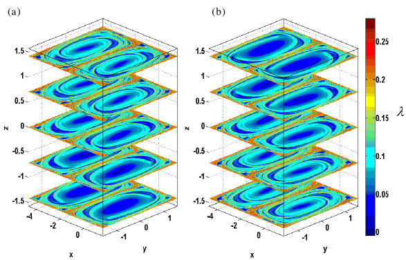
Figure 9: a) Forward and b) backward finite time Lyapunov exponent map on horizontal sections at $\tau=\pm 20\pi/\omega$ with parameter values $\epsilon_{0}=0.100$, $\epsilon_{1}=.008$ and $\omega=2.00$.

V.2.2 Lagrangian coherent structure

Recently, dynamically active barriers to transport labeled as Lagrangian Coherent Structures (LCS) have been revealed and studied in fluid flows Haller (2000); Haller and Yuan (2000); Haller (2001a, b). These structures are now seen to be crucial in understanding transport phenomena notably in time-dependent systems including oceanicLekien et al. (2005); Rypina et al. (2010), atmosphericTang et al. (2010) and physiological flowsShadden et al. (2010). These structures divide the fluid into dynamically distinct regions, revealing geometry hidden in the velocity field or trajectories of the system. These attractive and repulsive Lagrangian coherent structures can be defined as the ridges of the finite time Lyapunov exponent map calculated backward and forward in time.

Figure 10 presents these LCS that have been computed from the ridges of the forward and backward FTLE map (see Figs. 9). From these LCS that play the role of generalized attractive and repulsive manifolds (i.e. barriers to transport attracting or repulsing neighboring particles), the short time transport structures can be unambiguously revealed. From Fig. 10 we can see how the attractive (blue curve) and repulsive (red curve) LCS wind and tangle together. The attractive and repulsive LCS smoothly join together and wind around a surface starting from the bottom wall, passing around the vertical axis and finishing near the top wall. The fact that the attractive and repulsing LCS are smoothly joined and formed one curve ensures the presence of regular transport on this region and at this short time. Near the top wall and close to the vertical wall three hyperbolic structures separate the attractive and repulsive LCS (see Fig. 10). The attractive (or repulsive) LCS coming from the top (or bottom) wall begin to wander and tangle along the neighboring of the vertical walls, intersecting transversely the repulsive (attractive), thus indicating the presence of chaotic transport.

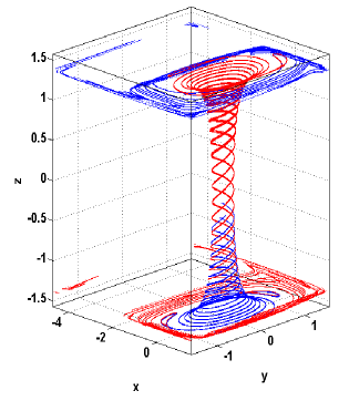
Figure 10: Attractive (blue) and repulsive (red) Lagrangian coherent structures inside a generic half-cell. Only a part of the attractive and repulsive LCS extension have been represented for clarity.

VI Conclusion

In this paper, we have exposed how the short-time differs from the long-time Lagrangian transport behavior for a three-dimensional time-dependent fluid model. More precisely, the model features are characteristic of oceanic flows and can be completely described by a set of three variables, one extremely slow, one slow and one fast. Contrary to most approaches that focus only on transport behavior at infinite time or averaged over time, we have turned our attention to the transport structures at short time. We have shown both qualitatively (using snapshots of the time evolution of advected particles) and quantitatively (using horizontal and vertical mixing index) the presence of specific short-time transport structures. In addition, using Lagrangian Coherent Structures we were able to identify and characterize these short-time transport structures. These short-time structures show strong and fast chaotic transport along vertical half-cell boundaries as well as seemingly regular transport around the half-cell vertical axis and near the top and bottom half-cell boundaries. These short-time structures contrast with the long-time behavior showing a spread-out chaotic transport throughout the cell. This knowledge of short-time transport structures is of great interest in numerous concrete applications, particularly for oceanic flows where simulations or observations are available only over a short time.

References

- Aharon et al. (2012) Aharon, R., V. Rom-Kedar, and H. Gildor (2012), Phys. Fluids 24 (5), 056603.
- Aref (2002) Aref, H. (2002), Phys. Fluids 14, 1315.
- Arnold (1963) Arnold, V. I. (1963), Russian Math. Survey 18, 13.
- Bajer and Moffatt (1990) Bajer, K., and H. Moffatt (1990), J. Fluid Mech. 212, 337.
- Cartwright et al. (1995) Cartwright, J. H. E., M. Feingold, and O. Piro (1995), Phys. Rev. Lett. 75, 3669.
- Cartwright et al. (1996) Cartwright, J. H. E., M. Feingold, and O. Piro (1996), J. Fluid Mech. 316, 259.
- Feingold et al. (1988) Feingold, M., L. P. Kadanoff, and O. Piro (1988), J. Stat. Phys. 50, 529.
- Haller (2000) Haller, G. (2000), Chaos 10, 99.
- Haller (2001a) Haller, G. (2001a), Physica D 149, 248.
- Haller (2001b) Haller, G. (2001b), Phys. Fluids 13, 3365.
- Haller and Yuan (2000) Haller, G., and G. Yuan (2000), Physica D 147, 352.
- Kolmogorov (1954) Kolmogorov, A. N. (1954), Dokl. Akad. Nauk. SSR 98, 527.
- Kroujiline and Stone (1999) Kroujiline, D., and H. A. Stone (1999), Physica D 130, 105.
- Lekien and Coulliette (2007) Lekien, F., and C. Coulliette (2007), Philos. Trans. R. Soc. A 365, 3061.
- Lekien et al. (2005) Lekien, F., et al. (2005), Physica D 210, 1.
- Liu and Yang (1994) Liu, Z., and H. Yang (1994), J. Phys. Oceanogr. 24, 1768.
- Mahadevan and Tandon (2006) Mahadevan, A., and A. Tandon (2006), Ocean Modelling 14 (3 4), 241 .
- Mancho et al. (2006) Mancho, A., D. Small, and S. Wiggins (2006), Phys. Rep. 437, 55.
- Mezić (2001) Mezić, I. (2001), Physica D 154, 51.
- Moser (1962) Moser, J. K. (1962), Nach. Akad. Wiss. G ttingen, Math. Phys. Kl. II, 1.
- Neishtadt (2005) Neishtadt, A. I. (2005), Tr. Mat. Inst. Steklova 250, 198.
- Paoletti et al. (2006) Paoletti, M., C. Nugent, and T. Solomon (2006), Phys. Rev. Lett. 96, 124101.
- Piro and Feingold (1988) Piro, O., and M. Feingold (1988), Phys. Rev. Lett. 61, 1799.
- Rypina et al. (2010) Rypina, I., et al. (2010), J. Phys. Oceanogr. 40, 1988.
- Samelson (1992) Samelson, R. (1992), J. Phys. Oceanogr. 22, 431 .
- Samelson and Wiggins (2010) Samelson, R., and S. Wiggins (2010), Lagrangian Transport in Geophysical Jets and Waves (Springer).
- Shadden et al. (2010) Shadden, S., M. Astorino, and J.-F. Gerbeau (2010), Chaos 20, 017512.
- Solomon and Gollub (1988a) Solomon, T. H., and J. P. Gollub (1988a), Phys. Rev. A 38, 6280.
- Solomon and Gollub (1988b) Solomon, T. H., and J. P. Gollub (1988b), Phys. Fluids 31, 1372.
- Stremler (2008) Stremler, M. A. (2008), in Encyclopedia of microfluidics and nanofluidics (Springer-Verlag, Germany).
- Tang et al. (2010) Tang, W., P. Chan, and G. Haller (2010), Chaos 20, 017502.
- Vainchtein et al. (2006) Vainchtein, D., A. Neishtadt, and I. Mezić (2006), Chaos 16, 043123.
- Vainchtein et al. (2007) Vainchtein, D. L., J. Widloski, and R. Grigoriev (2007), Phys. Rev. Lett. 99, 094501.
- Vainchtein et al. (2008) Vainchtein, D. L., J. Widloski, and R. O. Grigoriev (2008), Phys. Rev. E 78, 026302.
- Yan and Liu (1994) Yan, H., and Z. Liu (1994), Geophys. Res. Lett. 21, 545.