Generalized Slow Roll for Tensors

Abstract

The recent BICEP2 detection of degree scale CMB B-mode polarization, coupled with a deficit of observed power in large angle temperature anisotropy, suggest that the slow-roll parameter $\epsilon_{H}$, the fractional variation in the Hubble rate per efold, is both relatively large and may evolve from an even larger value on scales greater than the horizon at recombination. The relatively large tensor contribution implied also requires finite matching features in the tensor power spectrum for any scalar power spectrum feature proposed to explain anomalies in the temperature data. We extend the generalized slow-roll approach for computing power spectra, appropriate for such models where the slow-roll parameters vary, to tensor features where scalar features are large. This approach also generalizes the tensor-scalar consistency relation to be between the ratio of tensor and scalar sources and features in the two power spectra. Features in the tensor spectrum are generically suppressed by $\epsilon_{H}$ relative those in the scalar spectrum and by the smoothness of the Hubble rate, which must obey covariant conservation of energy, versus its derivatives. Their detection in near future CMB data would indicate a fast roll period of inflation where $\epsilon_{H}$ approaches order unity, allowed but not required by inflationary explanations of temperature anomalies.

I Introduction

The recent detection of inflationary tensor modes from $B$-mode polarization of the cosmic microwave background (CMB) by the BICEP2 experiment imply a large scalar to tensor ratio $r=0.2^{+0.07}_{-0.05}$ Ade et al. (2014) while also hinting at a violation of ordinary slow-roll prediction of a nearly scale-free curvature power spectrum. The latter is associated with the deficit rather than increment in the large angle Planck temperature power spectrum (e.g. Contaldi et al. (2014); Miranda et al. (2014); Abazajian et al. (2014); Hazra et al. (2014); Bousso et al. (2014)) which would imply $r<0.11$ (95% CL) in the standard cosmological constant, cold dark matter $\Lambda$CDM model Ade et al. (2013). Other hints of transient violations include glitches in the low multipole temperature spectrum Peiris et al. (2003) and high frequency oscillations in the high multipole temperature spectrum Flauger et al. (2010); Adshead et al. (2012); Ade et al. (2013).

Such violations also leave imprints on the tensor power spectrum. Generically tensor features require changes in the Hubble rate $H$ during inflation while scalar features only require changes in its derivatives or the inflaton sound speed. Order unity features would require order unity changes in $H$ and hence typically an interruption of inflation. Just like the tensor-scalar ratio itself, tensor features are suppressed relative to scalar features by a factor of the slow-roll parameter $\epsilon_{H}$, the fractional evolution of the Hubble parameter per efold (e.g. Hamann et al. (2007); Hazra et al. (2010)). On the other hand the relatively large $r$ implied by BICEP2 now requires a finite rather than infinitesimal $\epsilon_{H}$. It is therefore timely to develop general tools for the prediction of tensor features and study their consistency relation to scalar features.

The generalized slow-roll (GSR) approach was introduced in Ref. Stewart (2002); Choe et al. (2004); Gong (2004) to compute power spectra for models where the ordinary slow-roll parameters vary strongly with time but the background remains close to de Sitter. It was subsequently extended for order unity scalar power spectrum features Dvorkin and Hu (2010), for general single-field inflation Hu (2011) and for the curvature bispectrum Adshead et al. (2011, 2013).

Here we further develop these techniques for tensor power spectrum features and explore their relation to scalar power spectrum features in the limit that the latter are large. In §II, we extract the common mathematical structure of the GSR approach that is applicable to both scalars and tensors. In §III, we highlight the consistency relation, similarities and differences between scalar and tensor features. We provide examples in §IV motivated by anomalies in the temperature power spectrum and discuss these results in §V.

II Generalized Slow Roll

We begin by extracting the mathematical content of the GSR technique which is common to both scalar and tensor modes. As we shall see in §III, scalar curvature fluctuations and tensor gravitational waves satisfy a common evolution equation for their modefunctions $y$

$${d^{2}y\over dx^{2}}+\left(1-{2\over x^{2}}\right)y=\left(f^{\prime\prime}-3\frac{f^{\prime}}{f}\right)\frac{y}{x^{2}},$$ (1)

from Bunch-Davies initial conditions

$$\lim_{x\rightarrow\infty}y=e^{ix}.$$ (2)

Here ${}^{\prime}=d/d\ln x$ where $x$ is the time variable which for scalars will be associated with the sound horizon and for tensors the horizon; for both $x$ runs from infinity to zero as inflation progresses. Likewise scalars and tensors will have a different source of excitations from pure de Sitter conditions characterized by the time evolution of the function $f$. We shall see that $f$ in each case is related to the slow-roll parameters.

The GSR technique assumes that the excitations in the modefunctions are small rather the derivatives of $f$ itself, thus allowing the latter to evolve strongly due to inflationary features. Under this assumption, the modefunction equation can be solved iteratively by first setting the rhs of Eq. (1) to zero to obtain the de Sitter mode functions

$$y_{0}=\left(1+{i\over x}\right)e^{ix},$$ (3)

then replacing $y\rightarrow y_{0}$ in the rhs to solve for the first order correction $y_{1}$. This process may be repeated to arbitrary order. Iteration to second order yields for the superhorizon power

$$\Delta^{2} \equiv\lim_{x\rightarrow 0}\left|{\frac{xy}{f}}\right|^{2}$$

$$\approx e^{I_{0}}\left[\left(1+\frac{1}{4}I_{1}^{2}+\frac{1}{2}I_{2}\right)^{2}+\frac{1}{2}I_{1}^{2}\right].$$ (4)

Here the leading order term is

$$I_{0}=G(\ln x_{\rm min})+\int_{x_{\rm min}}^{\infty}{dx\over x}W(x)G^{\prime}(\ln x),$$ (5)

where $x_{\rm min}\ll 1$ and

$$G=-2\ln f+{2\over 3}(\ln f)^{\prime}$$ (6)

with ${}^{\prime}=d/d\ln x$. The window function

$$W(x)={3\sin(2x)\over 2x^{3}}-{3\cos(2x)\over x^{2}}-{3\sin(2x)\over 2x}$$ (7)

determines how the deviations from de Sitter freeze out. Note that this construction introduces $G^{\prime}$ in place of $f^{\prime\prime}-3f^{\prime}/f$ for these deviations so as to preserve the constancy of $|xy/f|$ above the horizon order by order, regardless of the size of $G^{\prime}$. Furthermore, in the ordinary slow-roll approximation, where $G$ is taken to be nearly constant $|xy/f|^{2}\rightarrow e^{G}\approx 1/f^{2}$, consistent with de Sitter modefunctions where $y_{0}\rightarrow i/x$. Thus we shall see that $1/f^{2}$ is associated with the scalar and tensor power spectra $\Delta^{2}$ in the ordinary slow-roll approximation.

The second order corrections are

$$I_{1} = {1\over\sqrt{2}}\int_{0}^{\infty}{dx\over x}G^{\prime}(\ln x)X(x),$$

$$I_{2} = -4\int_{0}^{\infty}{dx\over x}[X+{1\over 3}X^{\prime}]{f^{\prime}\over f}F_{2}(x),$$ (8)

with

$$X(x)={3\over x^{3}}(\sin x-x\cos x)^{2},$$ (9)

and

$$F_{2}(x)=\int_{x}^{\infty}{du\over u^{2}}{f^{\prime}\over f}.$$ (10)

The validity of the GSR expansion can be checked by calculating these corrections and ensuring that they are small compared with the leading order term.

III Tensors vs. Scalars

Now let us review the application of the GSR technique to scalar or comoving curvature fluctuations ${\cal R}$ and then apply it to tensors. The curvature modefunctions obey the evolution equation

$$\frac{d}{d\eta}\left(\frac{a^{2}\epsilon_{H}}{c_{s}^{2}}\frac{d{\cal R}}{d\eta}\right)+a^{2}\epsilon_{H}k^{2}{\cal R}=0,$$ (11)

where $c_{s}$ is the propagation or sound speed of the scalar fluctuations and can differ from unity if there are non-canonical kinetic terms in the inflaton Lagrangian. Deviations from a pure de Sitter expansion $H=$ const. are characterized by the slow-roll parameter

$$\epsilon_{H}=-\frac{d\ln H}{dN}.$$ (12)

The curvature modefunction equation (11) can be mapped onto the GSR modefunction equation (1) with the association Hu (2011)

$${\cal R}\equiv\sqrt{\frac{2\pi^{2}}{k^{3}}}\frac{x_{\cal R}y_{\cal R}}{f_{\cal R}}.$$ (13)

To distinguish scalar and tensor quantities, we append a subscript ${\cal R}$ to GSR variables involving scalars. Here $x_{\cal R}=ks$ where

$$s(N)=\int_{N}^{0}d\tilde{N}\frac{c_{s}}{aH}$$ (14)

is the sound horizon at an efold $N=\ln(a/a_{\rm end})$ from the end of inflation and

$$f_{\cal R}^{2} =\frac{8\pi^{2}\epsilon_{H}c_{s}}{H^{2}}\left(\frac{aHs}{c_{s}}\right)^{2}.$$ (15)

The GSR source for Eq. (5), $G_{\cal R}^{\prime}$, is a function of $\ln s$ independent of the wavenumber and ${}^{\prime}=d/d\ln x_{\cal R}=d/d\ln s$. The curvature power spectrum is defined as

$$\Delta_{\cal R}^{2}=\lim_{ks\rightarrow 0}\frac{k^{3}}{2\pi^{2}}|{\cal R}|^{2}=\lim_{x_{\cal R}\rightarrow 0}\left|\frac{x_{\cal R}y_{\cal R}}{f_{\cal R}}\right|^{2},$$ (16)

and so Eq. (4) says that to leading order

$$\ln\Delta_{\cal R}^{2}(k)\approx G_{\cal R}(\ln s_{\rm min})+\int_{s_{\rm min}}^{\infty}{ds\over s}W(ks)G_{\cal R}^{\prime}(\ln s).$$ (17)

Note that in the ordinary slow-roll approximation

$$G^{\prime}_{\cal R}\approx{\rm const.}\equiv 1-n_{S}\qquad{\rm(SR)},$$ (18)

and

$$\ln\Delta_{\cal R}^{2}(k)\approx G_{\cal R}(\ln s_{\rm min})+(n_{S}-1)[\ln(ks_{\rm min})-C]$$ (19)

consistent with a tilt of $n_{S}-1=d\ln\Delta_{\cal R}^{2}/d\ln k$ where $C=7/3-\gamma_{E}-\ln 2$ with $\gamma_{E}$ as the Euler-Mascheroni constant.

Next consider the tensor fluctuations which represent gravitational wave amplitudes $h_{+,\times}$. Their modefunction equation, for either polarization and wavenumbers much smaller than the curvature scale, is

$$\frac{d^{2}h}{d\eta^{2}}+\frac{2}{a}\frac{da}{d\eta}\frac{dh}{d\eta}+k^{2}h=0,$$ (20)

where

$$\eta(N)=\int_{N}^{0}d\tilde{N}\frac{1}{aH}$$ (21)

is the horizon measured from the end of inflation. The gravitational wave modefunction is related to $y_{h}$ through canonical normalization

$$h\equiv\sqrt{\frac{2\pi^{2}}{k^{3}}}\frac{x_{h}y_{h}}{f_{h}},$$ (22)

with Gong (2004)

$$f_{h}^{2} =\frac{2\pi^{2}}{H^{2}}\left({aH\eta}\right)^{2}\propto(a\eta)^{2},$$ (23)

which transforms Eq. (20) into the modefunction equation Eq. (1) with the association

$$f_{h}^{\prime\prime}-3\frac{f_{h}^{\prime}}{f_{h}}=\frac{\eta^{2}}{a}\frac{d^{2}a}{d\eta^{2}}-2.$$ (24)

Thus the tensor power spectrum in each polarization state is

$$\Delta_{+,\times}^{2}=\lim_{k\eta\rightarrow 0}\frac{k^{3}}{2\pi^{2}}|h|^{2}=\lim_{x\rightarrow 0}\left|\frac{x_{h}y_{h}}{f_{h}}\right|^{2}$$ (25)

and Eq. (4) determines how deviations in the source function $G^{\prime}_{h}$ freeze out. Explicitly, to leading order

$$\ln\Delta_{+,\times}^{2}(k)\approx G_{h}(\ln\eta_{\rm min})+\int_{\eta_{\rm min}}^{\infty}{d\eta\over\eta}W(k\eta)G_{h}^{\prime}(\ln\eta),$$ (26)

where in distinction to scalars ${}^{\prime}=d/d\ln x_{h}=d/d\ln\eta$ and

$$G^{\prime}_{h}=-2(1-aH\eta)-\frac{2}{3}aH\eta\left(1-aH\eta+aH\eta\,\epsilon_{H}\right).$$ (27)

In the ordinary slow-roll approximation $aH\eta\approx 1+\epsilon_{H}$ and hence

$$G^{\prime}_{h}\approx 2\epsilon_{H}=-n_{T}\qquad{\rm(SR)},$$ (28)

which yields

$$\ln\Delta_{+,\times}^{2}(k)\approx G_{h}(\ln\eta_{\rm min})+n_{T}[\ln(k\eta_{\rm min})-C]$$ (29)

consistent with $n_{T}=d\ln\Delta^{2}_{+,\times}/d\ln k$ as the tensor tilt. Note that even beyond the constant $\epsilon_{H}$ approximation

$$(1-aH\eta)={\cal O}(\epsilon_{H}),$$ (30)

and hence $G^{\prime}_{h}={\cal O}(\epsilon_{H})$.

There are several similarities and difference between scalars and tensors in the context of inflationary features that are worth highlighting. In place of the direct consistency relation between the tensor-scalar ratio and the tilt of the tensor power spectrum is a relationship between the GSR source functions

$$r_{f}\equiv 4\frac{f_{{\cal R}}^{2}}{f_{h}^{2}}=16{\epsilon_{H}c_{s}}\left(\frac{s}{c_{s}\eta}\right)^{2}.$$ (31)

Recall that in the slow-roll approximation $1/f^{2}$ is directly related to the corresponding power spectrum and $s\approx c_{s}\eta$ so that

$$r_{f}\approx\frac{4\Delta^{2}_{+,\times}}{\Delta^{2}_{\cal R}}\equiv r\approx 16\epsilon_{H}c_{s}\qquad{\rm(SR)},$$ (32)

which in turn is related to the tilt of the tensor spectrum in slow roll through Eq. (28). Beyond the ordinary slow-roll limit of constant $G^{\prime}$, the consistency relation (31) still implies that the GSR $f$ sources, and hence power spectrum features, are related. However their appearance in the respective power spectra goes through the freezeout integrals over $G^{\prime}$ rather than simply the tensor tilt.

Freezeout occurs at different epochs for tensors than scalars. For example a feature at some common efold $N_{s}$ induces changes to the ${\cal R}$ and $h$ modefunctions if $k\gtrsim 1/\eta(N_{s})$ for tensors but only if $k\gtrsim 1/s(N_{s})$ for scalars. Hence for $c_{s}\ll 1$, there is a range of wavenumbers where a feature can impact tensors while not affecting scalars which have already passed through the sound horizon.

Next only features in the evolution of $H$ or equivalently $\epsilon_{H}$ affect tensors whereas features in $c_{s}$ also affect scalars. Moreover, features in $\epsilon_{H}$ impact scalars more than they do tensors as long as $\epsilon_{H}\ll 1$, the requirement of a near de Sitter expansion which is at the heart of both the ordinary and generalized slow-roll approximations. Energy conservation guarantees that $H$ evolves continuously and energy loss to the expansion can only occur on the efold time scale.

The tensor GSR sources therefore yield $O(\Delta\epsilon_{H})$ fractional effects on top of the slow-roll power spectrum through $G^{\prime}_{h}$, whereas the scalar GSR sources produce $O(\Delta\epsilon_{H}/\epsilon_{H})$ fractional effects. Thus we generically expect tensor power spectrum features to be suppressed relative to scalar power spectrum features by at least a factor of $\epsilon_{H}$.

The BICEP2 result suggests that tensor to scalar ratio $r\approx 0.2$ and so $\epsilon_{H}\sim 0.2/16c_{s}$ during the slow-roll period. For canonical sound speed models $c_{s}=1$ and we generically expect features in the tensor sector to be percent level for order unity scalar features. For low sound speed models, the effect can be larger but only at the expense of making $\epsilon_{H}$ larger which in turn limits the number of efolds that slow-roll inflation can proceed. Thus tensor features that are comparable to scalar features typically require a short duration fast roll period of inflation where $\epsilon_{H}$ itself reaches order unity. While a truly fast roll period would also suppress scalar fluctuations on large scales and assist in reconciling the BICEP2 result with upper limits on $r$ from Planck, we shall show in the next section it is not required to resolve this tension.

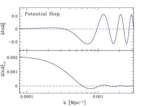
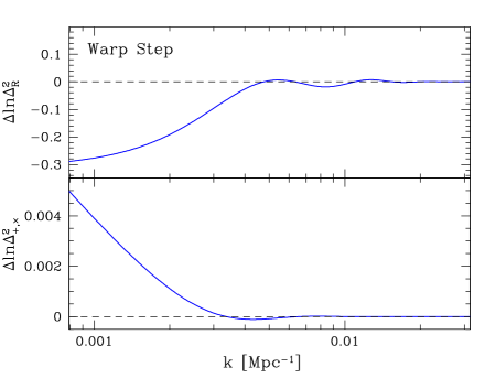
Figure 1: Examples of scalar and tensor features. Left: extremely sharp potential step that fits high frequency oscillations in the Planck temperature anisotropy data. Right: warp step that fits the scalar suppression implied by the BICEP2 $B$-mode detection and the Planck large angle temperature power spectrum. In both cases, tensor features are suppressed by a factor of $\epsilon_{H}\ll 1$ and oscillations are further suppressed by the relative smoothness of the tensor source due to energy conservation.

IV Examples

Features in the scalar and tensor power spectra arise from the evolution of $\epsilon_{H}$ and $c_{s}$ which excite the scalar and tensor modefunctions from their de Sitter forms. We have seen in the previous section that tensor features are generically small so long as the background is nearly de-Sitter or $\epsilon_{H}\ll 1$, even if the evolution of $\epsilon_{H}$ is strong enough to induce large scalar features $\Delta\epsilon_{H}/\epsilon_{H}={\cal O}(1)$. In this section we quantify this expectation with concrete models that are motivated by features in the observed CMB temperature power spectrum Miranda and Hu (2014); Miranda et al. (2014).

These models involve sharp steps in for example the potential or warp factor of DBI inflation, including its $c_{s}\rightarrow 1$ limit of a canonical scalar field inflaton. Following Miranda et al. (2012); Miranda and Hu (2014), the evolution of $\epsilon_{H}$ and $c_{s}$ is generically quantified by the change in their values from before (“$b$”) to immediately following the step (“$i$”), as determined by energy conservation, and then their decay back to their inflationary attractor values (“$a$”) several efolds after the step. It is convenient to normalize the former quantities to the values $\epsilon_{Ha}$ and $c_{sa}$ after the step leaving the free parameters

$$e_{b} = \frac{\epsilon_{Hb}}{\epsilon_{Ha}},\qquad e_{i}=\frac{\epsilon_{Hi}}{\epsilon_{Ha}},$$

$$c_{b} = \frac{c_{sb}}{c_{sa}},\qquad\ c_{i}=\frac{c_{si}}{c_{sa}}.$$ (33)

Let us represent the step itself with the function $F$, which takes on the value $-2$ before the step $N<N_{s}$ and $0$ after the step $N>N_{s}$. Then the evolution across the step becomes

$$\frac{c_{s}}{c_{sa}}(N)= 1+\frac{1-c_{b}}{2}F+\frac{c_{i}-1}{2}(F+2)e^{3(N_{s}-N)},$$ (34)

$$\frac{\epsilon_{H}}{\epsilon_{Ha}}(N)= 1+\frac{1-e_{b}}{2}F+\frac{e_{i}-1}{2}(F+2)e^{3(N_{s}-N)}.$$

$G_{{\cal R}}^{\prime}$ and $G_{h}^{\prime}$ can then be computed by taking derivatives and integrals of these fundamental quantities. By defining $H$ through the integral of $\epsilon_{H}$ we guarantee energy conservation which is crucial in establishing its continuous evolution in the presence of the step.

To leading order, the change in the scalar power spectrum due to the step is Miranda et al. (2012)

$$\Delta\ln\Delta_{\mathcal{R}}^{2}= C_{1}W(ks_{s})+C_{2}W^{\prime}(ks_{s})+C_{3}Y(ks_{s}),$$ (35)

where

$$Y(x) =\frac{6x\cos(2x)+(4x^{2}-3)\sin(2x)}{x^{3}},$$ (36)

and Miranda and Hu (2014)

$$C_{1} =-\ln c_{b}e_{b},$$

$$C_{2} =-\frac{2}{3}\frac{c_{i}-c_{b}}{c_{i}+c_{b}}+\frac{2}{3}\frac{e_{i}-e_{b}}{e_{i}+e_{b}},$$

$$C_{3} =2\frac{(1-c_{b})+(c_{i}-1)/4}{c_{i}+c_{b}},$$ (37)

and we have assumed $\epsilon_{Ha}\ll 1$. The $W$ term represents a step in the scalar power spectrum due to change in $\epsilon_{H}c_{s}$. The $W^{\prime}$ term produces constant amplitude ringing in the power spectrum as the transfer of an infinitely sharp step. The $Y$ term alters the spectrum around $ks_{s}=1$ by enhancing the sharpness of the step.

For the tensor spectrum, a similar series of calculations yields

$$\Delta\ln\Delta_{+,\times}^{2}= B_{1}W(k\eta_{s})+B_{2}V(k\eta_{s})+B_{3}Y(k\eta_{s}),$$ (38)

where

$$V(x) =\int_{x}^{\infty}\frac{d\tilde{x}}{\tilde{x}}W(\tilde{x})$$

$$=\frac{(1+x^{2})\sin(2x)-2x\cos(2x)}{2x^{3}}-{\rm Ci}(2x),$$ (39)

with Ci as the cosine integral and

$$B_{1} =\frac{8}{3}\left[(1-e_{b})+\frac{1}{4}(e_{i}-1)\right]\epsilon_{Ha},$$

$$B_{2} =2(e_{b}-1)\epsilon_{Ha},$$

$$B_{3} =\left[(1-e_{b})+\frac{1}{4}(e_{i}-1)\right]\epsilon_{Ha}.$$ (40)

Note that in comparison with the $C_{i}$ scalar amplitudes, the $B_{i}$ tensor amplitudes are all suppressed by a factor of $\epsilon_{Ha}$ as discussed in the previous section.

The new $V$ term here has the limit

$$\lim_{x\rightarrow 0}V(x)=C-\ln x,$$ (41)

where $C$ was defined in Eq. (19) and induces an effect similar to a change in the tensor tilt since $dV/d\ln k=dV/d\ln x$. Indeed the difference between $\epsilon_{Hb}$ and $\epsilon_{Ha}$ represented by a finite $e_{b}-1$ changes the tensor tilt according to Eq. (28) in the slow-roll attractors away from step. While it induces a similar effect on the scalar spectrum, the other $C_{i}$ effects are zeroth order effects in $\epsilon_{Ha}$ whereas all tensor $B_{i}$ effects begin at first order.

Finally for a finite width step, the oscillatory features in both spectra are damped at high wavenumbers due to the fact that the $W$ window function oscillates many times while the step is being traversed. In the sharp step limit where this duration is still much less than an efold $x_{d}\approx 1/\delta N\gg 1$, the $\Delta\ln\Delta^{2}$ power spectrum deviations of Eq. (35) and (38) are multiplied by a damping envelope ${\cal D}(x/x_{d})$ which for a Tanh step is Adshead et al. (2012)

$${\cal D}(y)=\frac{y}{\sinh y}.$$ (42)

For explicit examples, we first take the sharp step in the potential at $s_{s}=\eta_{s}=3696.9$Mpc with $x_{d}\gg 1$ that fits high frequency oscillations in the Planck temperature power spectrum at high multipole from Ref. Miranda and Hu (2014). For simplicity we take the limit of a canonical scalar field $c_{s}=c_{sa}=1$ and a tensor-scalar ratio $r=0.2$ after the step as consistent with BICEP2. Hence

$$\epsilon_{Ha} =\frac{0.2}{16}=0.0125,$$ (43)

and for the best fit amplitude

$$e_{i} =1.254,$$

$$c_{b} =c_{i}=e_{b}=1.$$ (44)

Note that for a potential step, $\epsilon_{H}$ returns to the same value to leading order well after the step $(e_{b}=1)$.

The scalar and tensor power spectrum features for this model are shown in Fig. 1 (left). Since $c_{s}=1$, $\eta_{s}=s_{s}$ and the location of the features align but the maximum amplitude of the tensor relative to the scalar features scales as $\epsilon_{Ha}$. Moreover, the tensor features lack the high $k$ constant oscillations from $W^{\prime}$ that make the scalars observable given the decrease in the associated cosmic variance. Despite the sharp step in the potential, energy conservation forbids a sharp step in $H$ and hence unlike the scalars there is no ringing out to high $k$.

In fact, oscillatory features at high $k$ in tensors are even further suppressed in the observable CMB B-mode polarization due to the much broader projection of power from $k$ to multipole $\ell$ associated with B-mode tensor polarization as compared with temperature or E-mode scalar perturbations Hu and White (1997). Combined these facts imply that the tensor features associated with this model are too small to be observed.

Next consider a step in the DBI warp that causes a similar step in the quantity $\epsilon_{H}c_{s}$ and consequently the scalar power spectrum. The implied reduction of large scale scalar power fits the Planck temperature anisotropy data while allowing a large $r=0.2$ tensor contribution to explain the BICEP2 result Miranda et al. (2014). For simplicity, we again take $c_{sb}=c_{b}c_{sa}=1$ and choose parameters to fit the amplitude and shape of the required reduction

$$c_{sa} =1/c_{b}=0.856,$$

$$\epsilon_{Ha} =\frac{0.2}{16c_{sa}}=0.0146,$$

$$x_{d} =1.43.$$ (45)

Note that this small an $x_{d}$ does not represent a step that is traversed in much less than an efold making the sharp step assumption in evaluating GSR integrals only approximate; however comparisons with the exact scalar calculation show that this approximation suffices for the description here since even without damping, tensor oscillatory features are suppressed relative to scalars as we have seen in the previous example. This model determines the evolution of $c_{s}$ and $\epsilon_{H}$ by setting

$$c_{b} =e_{b}\approx 1/c_{sa}=1.168,$$

$$c_{i} =0.988,$$

$$e_{i} =1.078.$$ (46)

Fig. 1 (right) shows the associated scalar and tensor features. Again the overall scale of tensor feature is reduced by $\epsilon_{H}$ compared with the scalar feature. In this case, $\epsilon_{H}$ itself undergoes a step-like change across the feature and hence the logarithmic rise at small $k$ in the tensor spectrum is due to the change in tensor tilt in the slow-roll regime before the feature. However the cosmic variance of low $k$ modes and the finite size of the current horizon prevents this effect from being measurable. In this case the large width of the step, represented by $x_{d}$, damps oscillatory features in both scalars and tensors. Note that the location of oscillatory features are at slightly smaller $k$ since $\eta_{s}>s_{s}$. Again the combination of these facts imply that tensor features associated with this model are too small to be observable.

The common feature of these two examples is that while the ordinary slow-roll approximation ($\epsilon_{H}\approx$ const.) is strongly violated, slow roll itself is never violated ($\epsilon_{H}\ll 1$). Thus they illustrate the fact that large and potentially observable tensor features requires a fast roll period of inflation.

V Discussion

In this work, we have developed the generalized slow-roll formalism for tensor power spectrum features from transient violations of the ordinary slow-roll approximation. Here the slow-roll parameters are not assumed to be constant and only the background expansion is assumed to be nearly de Sitter or time translation invariant. Generally, features in the scalar power spectrum imply a corresponding set of features in the tensor power spectrum governed by a generalized consistency relation between their sources. However, the amplitude of tensor features is suppressed by the slow-roll factor $\epsilon_{H}$ relative to scalar features and also do not generate as large oscillatory features at high wavenumber since the evolution of $H$ is governed by energy conservation and smoother than its derivatives.

As an illustration of this behavior, we considered inflationary features that are motivated by anomalies the CMB temperature data, namely high frequency variations at high multipole moment in the Planck data and a step suppression of power at low multipoles. Preference for the latter is substantially strengthened by the BICEP2 detection of tensor contributions to $B$-mode polarization. While explanations of either anomaly imply a matching set of tensor features, neither require a fast roll period where $\epsilon_{H}={\cal O}(1)$ and in the absence of such a period, tensor features are greatly suppressed compared with scalar features.

A fast roll period is nonetheless possible if confined to efolds just prior to when the current horizon exited the horizon during inflation. For example, these efolds could represent the end of a prior period of kinetic energy domination Contaldi et al. (2003); Lello and Boyanovsky (2013). Hence the observation of tensor features could provide support for such models and distinguish them from slow-roll alternatives that similarly suppress large scale temperature power.

More generally, model independent reconstruction of the scalar and tensor source functions $G^{\prime}_{{\cal R}}$ and $G^{\prime}_{h}$ could test the consistency of slow-roll inflation more generally than the ordinary slow-roll consistency relation Dvorkin and Hu (2011). Observable deviations from constant $G^{\prime}_{h}$ require substantial evolution in the Hubble rate, a violation of time-translation invariance, from a relatively fast roll period. The GSR approach should be useful for calculating the tensor spectrum of such models out to scales approaching the beginning of the main inflationary period where order unity variations are possible.

Acknowledgments: WH thanks Peter Adshead for useful conversations and CosKASI where this work was initiated. This work was supported by the Kavli Institute for Cosmological Physics at the University of Chicago through grants NSF PHY-1125897 and an endowment from the Kavli Foundation and its founder Fred Kavli and by U.S. Dept. of Energy contract DE-FG02-13ER41958.

References

- Ade et al. (2014) P. Ade et al. (BICEP2 Collaboration), (2014), arXiv:1403.3985 [astro-ph.CO] .
- Contaldi et al. (2014) C. R. Contaldi, M. Peloso, and L. Sorbo, (2014), arXiv:1403.4596 [astro-ph.CO] .
- Miranda et al. (2014) V. Miranda, W. Hu, and P. Adshead, (2014), arXiv:1403.5231 [astro-ph.CO] .
- Abazajian et al. (2014) K. N. Abazajian, G. Aslanyan, R. Easther, and L. C. Price, (2014), arXiv:1403.5922 [astro-ph.CO] .
- Hazra et al. (2014) D. K. Hazra, A. Shafieloo, G. F. Smoot, and A. A. Starobinsky, (2014), arXiv:1404.0360 [astro-ph.CO] .
- Bousso et al. (2014) R. Bousso, D. Harlow, and L. Senatore, (2014), arXiv:1404.2278 [astro-ph.CO] .
- Ade et al. (2013) P. Ade et al. (Planck Collaboration), (2013), arXiv:1303.5082 [astro-ph.CO] .
- Peiris et al. (2003) H. Peiris et al. (WMAP Collaboration), Astrophys.J.Suppl., 148, 213 (2003), arXiv:astro-ph/0302225 [astro-ph] .
- Flauger et al. (2010) R. Flauger, L. McAllister, E. Pajer, A. Westphal, and G. Xu, JCAP, 1006, 009 (2010), arXiv:0907.2916 [hep-th] .
- Adshead et al. (2012) P. Adshead, C. Dvorkin, W. Hu, and E. A. Lim, Phys.Rev., D85, 023531 (2012), arXiv:1110.3050 [astro-ph.CO] .
- Hamann et al. (2007) J. Hamann, L. Covi, A. Melchiorri, and A. Slosar, Phys. Rev., D76, 023503 (2007), arXiv:astro-ph/0701380 .
- Hazra et al. (2010) D. K. Hazra, M. Aich, R. K. Jain, L. Sriramkumar, and T. Souradeep, JCAP, 1010, 008 (2010), arXiv:1005.2175 [astro-ph.CO] .
- Stewart (2002) E. D. Stewart, Phys.Rev., D65, 103508 (2002), arXiv:astro-ph/0110322 [astro-ph] .
- Choe et al. (2004) J. Choe, J.-O. Gong, and E. D. Stewart, JCAP, 0407, 012 (2004), arXiv:hep-ph/0405155 .
- Gong (2004) J.-O. Gong, Class.Quant.Grav., 21, 5555 (2004), arXiv:gr-qc/0408039 [gr-qc] .
- Dvorkin and Hu (2010) C. Dvorkin and W. Hu, Phys. Rev., D81, 023518 (2010), arXiv:0910.2237 [astro-ph.CO] .
- Hu (2011) W. Hu, Phys.Rev., D84, 027303 (2011), arXiv:1104.4500 [astro-ph.CO] .
- Adshead et al. (2011) P. Adshead, W. Hu, C. Dvorkin, and H. V. Peiris, Phys.Rev., D84, 043519 (2011), arXiv:1102.3435 [astro-ph.CO] .
- Adshead et al. (2013) P. Adshead, W. Hu, and V. Miranda, Phys.Rev., D88, 023507 (2013), arXiv:1303.7004 [astro-ph.CO] .
- Miranda and Hu (2014) V. Miranda and W. Hu, Phys.Rev., D89, 083529 (2014), arXiv:1312.0946 [astro-ph.CO] .
- Miranda et al. (2012) V. Miranda, W. Hu, and P. Adshead, Phys.Rev., D86, 063529 (2012), arXiv:1207.2186 [astro-ph.CO] .
- Hu and White (1997) W. Hu and M. J. White, Phys.Rev., D56, 596 (1997), arXiv:astro-ph/9702170 [astro-ph] .
- Contaldi et al. (2003) C. R. Contaldi, M. Peloso, L. Kofman, and A. D. Linde, JCAP, 0307, 002 (2003), arXiv:astro-ph/0303636 [astro-ph] .
- Lello and Boyanovsky (2013) L. Lello and D. Boyanovsky, (2013), arXiv:1312.4251 [astro-ph.CO] .
- Dvorkin and Hu (2011) C. Dvorkin and W. Hu, Phys.Rev., D84, 063515 (2011), arXiv:1106.4016 [astro-ph.CO] .