Improved Distributed Steiner Forest Construction

We present new distributed algorithms for constructing a Steiner Forest in the congest model. Our deterministic algorithm finds, for any given constant $\varepsilon>0$, a $(2+\varepsilon)$-approximation in $\tilde{\mathcal{O}}(sk+\sqrt{\min\left\{st,n\right\}})$ rounds, where $s$ is the “shortest path diameter,” $t$ is the number of terminals, and $k$ is the number of terminal components in the input. Our randomized algorithm finds, with high probability, an $\mathcal{O}(\log n)$-approximation in time $\tilde{\mathcal{O}}(k+\min\left\{s,\sqrt{n}\right\}+D)$, where $D$ is the unweighted diameter of the network. We prove a matching lower bound of $\tilde{\Omega}(k+\min\left\{s,\sqrt{n}\right\}+D)$on the running time of any distributed approximation algorithm for the Steiner Forest problem. The best previous algorithms were randomized and obtained either an $\mathcal{O}(\log n)$-approximation in $\tilde{\mathcal{O}}(sk)$ time, or an $\mathcal{O}(1/\varepsilon)$-approximation in $\tilde{\mathcal{O}}((\sqrt{n}+t)^{1+\varepsilon}+D)$ time.

1 Introduction

Ever since the celebrated paper of Gallager, Humblet, and Spira [10], the task of constructing a minimum-weight spanning tree (MST) continues to be a rich source of difficulties and ideas that drive network algorithmics (see, e.g., [9, 11, 18, 20]). The Steiner Forest (SF) problem is a strict generalization of MST: We are given a network with edge weights and some disjoint node subsets called input components; the task is to find a minimum-weight edge set which makes each component connected. MST is a special case of SF, and so are the Steiner Tree and shortest $s$-$t$ path problems. The general SF problem is well motivated by many practical situations involving the design of networks, be it physical (it was famously posed as a problem of railroad design), or virtual (e.g., VPNs or streaming multicast). The problem has attracted much attention in the classical algorithms community, as detailed on the dedicated website [12].

The first network algorithm for SF in the congest model (where a link can deliver $\mathcal{O}(\log n)$ bits in a time unit—details in Section 2) was presented by Khan et al. [14]. It provides $\mathcal{O}(\log n)$-approximate solutions in time $\tilde{\mathcal{O}}(sk)$, where $n$ is the number of nodes, $k$ is the number of components, and $s$ the shortest path diameter of the network, which is (roughly—see Section 2) the maximal number of edges in a weighted shortest path. Subsequently, in [17], it was shown that for any given $0<\varepsilon\leq 1/2$, an $\mathcal{O}(\varepsilon^{-1})$-approximate solution to SF can be found in time $\tilde{\mathcal{O}}((\sqrt{n}+t)^{1+\varepsilon}+D)$, where $D$ is the diameter of the unweighted version of the network, and $t$ is the number of terminals, i.e., the total number of nodes in all input components. The algorithms in [14, 17] are both randomized.

Our Results.

In this paper we improve the results for SF in the congest model in two ways. First, we show that for any given constant $\varepsilon>0$, a $(2+\varepsilon)$-approximate solution to SF can be computed by a deterministic network algorithm in time $\tilde{\mathcal{O}}(sk+\sqrt{\min\left\{st,n\right\}})$. Second, we show that an $\mathcal{O}(\log n)$-approximation can be attained by a randomized algorithm in time $\tilde{\mathcal{O}}(k+\min\left\{s,\sqrt{n}\right\}+D)\subseteq\tilde{\mathcal{O}}(s+k)$. On the other hand, we show that any algorithm in the congest model that computes a solution to SF with non-trivial approximation ratio has running time in $\tilde{\Omega}(k+\min\left\{s,\sqrt{n}\right\}+D)$. If the input is not given by indicating to each terminal its input component, but rather by connection requests between terminals, i.e., informing each terminal which terminals it must be connected to, an $\tilde{\Omega}(t+\min\left\{s,\sqrt{n}\right\}+D)$ lower bound holds. (It is easy to transform connection requests into equivalent input components in $\mathcal{O}(t+D)$ rounds.)

Related work.

The Steiner Tree problem (the special case of SF where there is one input component) has a remarkable history, starting with Fermat, who posed the geometric 3-point on a plane problem circa 1643, including Gauss (1836), and culminating with a popularization in 1941 by Courant and Robbins in their book “What is Mathematics” [7]. An interesting account of these early developments is given in [2]. The contribution of Computer Science to the history of the problem apparently started with the inclusion of Steiner Tree as one of the original 21 problems proved NP-complete by Karp [13]. There are quite a few variants of the SF problem which are algorithmically interesting, such as Directed Steiner Tree, Prize-Collecting Steiner Tree, Group Steiner Tree, and more. The site [12] gives a continuously updated state of the art results for many variants. Let us mention results for just the most common variants: For the Steiner Tree problem, the best (polynomial-time) approximation ratio known is $\ln 4+\varepsilon\approx 1.386+\varepsilon$ for any constant $\varepsilon>0$ [3]. For Steiner Forest, the best approximation ratio known is $2-1/(t-k)$ [1]. It is also known that the approximation ratio of the Steiner Tree (or Forest) problem is at least $96/95$, unless P=NP [5].

Regarding distributed algorithms, there are a few relevant results. First, the special case of minimum-weight spanning tree (MST) is known to have time complexity of $\tilde{\Theta}(D+\sqrt{n})$ in the congest model [8, 9, 11, 16, 20]. In [4], a 2-approximation for the special case of Steiner Tree is presented, with time complexity $\tilde{\mathcal{O}}(n)$. The first distributed solution to the Steiner Forest problem was presented by Khan et al. [14], where a randomized algorithm is used to embed the instance in a virtual tree with $\mathcal{O}(\log n)$ distortion, then finding the optimal solution on the tree (which is just the minimal subforest connecting each input component), and finally mapping the selected tree edges back to corresponding paths in the original graph. The result is an $\mathcal{O}(\log n)$-approximation in time $\tilde{\mathcal{O}}(sk)$. Intuitively, $s$ is the time required by the Bellman-Ford algorithm to compute distributed single-source shortest paths, and the virtual tree of [14] is computed in $\tilde{\mathcal{O}}(s)$ rounds. A second distributed algorithm for Steiner Forest is presented in [17]. Here, a sparse spanner for the metric induced on the set of terminals and a random sample of $\tilde{\Theta}(\sqrt{n})$ nodes is computed, on which the instance then is solved centrally. To get an $\mathcal{O}(\varepsilon^{-1})$-approximation, the algorithm runs for $\tilde{\mathcal{O}}(D+(\sqrt{n}+t)^{1+\varepsilon})$ rounds. For approximation ratio $\mathcal{O}(\log n)$, the running time is $\tilde{\mathcal{O}}(D+\sqrt{n}+t)$.

Main Techniques.

Our lower bounds are derived by the standard technique of reduction from results on $2$-party communication complexity. Our deterministic algorithm is an adaptation of the “moat growing” algorithm of Agrawal, Klein, and Ravi [1] to the congest model. It involves determining the times in which “significant events” occur (e.g., all terminals in an input component becoming connected by the currently selected edges) and extensive usage of pipelining. The algorithm generalizes the MST algorithm from [16]: for the special case of a Steiner Tree (i.e., $k=1$), one can interpret the output as the edge set induced by an MST of the complete graph on the terminals with edge weights given by the terminal-terminal distances, yielding a factor-$2$ approximation; specializing further to the MST problem, the result is an exact MST and the running time becomes $\tilde{\mathcal{O}}(\sqrt{n}+D)$.

Our randomized algorithm is based on the embedding of the graph into a tree metric from [14], but we improve the complexity of finding a Steiner Forest. A key insight is that while the least-weight paths in the original graph corresponding to virtual tree edges might intersect, no node participates in more than $\mathcal{O}(\log n)$ distinct paths. Since the union of all least-weight paths ending at a specific node induces a tree, letting each node serve routing requests corresponding to different destinations in a round-robin fashion achieves a pipelining effect reducing the complexity to $\tilde{\mathcal{O}}(s+k)$. If $s>\sqrt{n}$, the virtual tree and the corresponding solution are constructed only partially, in time $\tilde{\mathcal{O}}(\sqrt{n}+k+D)$, and the partial result is used to create another instance with $\mathcal{O}(\sqrt{n})$ terminals that captures the remaining connectivity demands; we solve it using the algorithm from [17], obtaining an $\mathcal{O}(\log n)$-approximation.

Organization.

In Section 2 we define the model, problem and basic concepts. Section 3 contains our lower bounds. In Section 4 and Section 5 we present our deterministic and randomized algorithms, respectively. We only give a high-level overview in this extended abstract. Proofs are deferred to the appendix.

2 Model and Notation

System Model.

We consider the $\textsc{congest}(\log n)$ or simply the congest model as specified in [19], briefly described as follows. The distributed system is represented by a weighted graph $G=(V,E,W)$ of $n:=|V|$ nodes. The weights $W:E\to\mathbb{N}$ are polynomially bounded in $n$ (and therefore polynomial sums of weights can be encoded with $\mathcal{O}(\log n)$ bits). Each node initially knows its unique identifier of $\mathcal{O}(\log n)$ bits, the identifiers of its neighbors, the weight of its incident edges, and the local problem-specific input specified below. Algorithms proceed in synchronous rounds, where in each round, (i) nodes perform arbitrary, finite local computations, (ii) may send, to each neighbor, a possibly distinct message of $\mathcal{O}(\log n)$ bits, and (iii) receive the messages sent by their neighbors. For randomized algorithms, each node has access to an unlimited supply of unbiased, independent random bits. Time complexity is measured by the number of rounds until all nodes (explicitly) terminate.

Notation.

We use the following conventions and graph-theoretic notions.

• The length or number of hops of a path $p=(v_{0},\ldots,v_{\ell(p)})$ in $G$ is $\ell(p)$.

• The weight of such a path is $W(p):=\sum_{i=1}^{\ell(p)}W(v_{i},v_{i-1})$. For notational convenience, we assume w.l.o.g. that different paths have different weight (ties broken lexicographically).

• By $\operatorname{{\cal P}}(v,w)$ we denote the set of all paths between $v,w\in V$ in $G$, i.e., $v_{0}=v$ and $v_{\ell(p)}=w$.

• The (unweighted) diameter of $G$ is
  $D:=\max_{v,w\in V}\{\min_{p\in\operatorname{{\cal P}}(v,w)}\{\ell(p)\}\}$.

• The (weighted) distance of $v$ and $w$ in $G$ is $\operatorname{wd}(v,w):=\min_{p\in\operatorname{{\cal P}}(v,w)}\{W(p)\}$.

• The weighted diameter of $G$ is $\operatorname{WD}:=\max_{v,w\in V}\{\operatorname{wd}(v,w)\}$.

• Its shortest-path-diameter is $s:=\max_{v,w\in V}\{\min\{\ell(p)\,|\,p\in\operatorname{{\cal P}}(v,w)\wedge W(p)=\operatorname{wd}(v,w)\}\}$.

• For $v\in V$ and $r\in\mathbb{R}^{+}_{0}$, we use $B_{G}(v,r)$ to denote the ball of radius $r$ around $v$ in $G$, which includes all nodes and edges at weighted distance at most $r$ from $v$. The ball may contain edge fractions: for an edge $\{w,u\}$ for which $w$ is in $B_{G}(v,r)$, the $(r-\operatorname{wd}(v,w))/\operatorname{wd}(v,w)$ fraction of the edge closer to $w$ is considered to be within $B_{G}(v,r)$, and the remainder is considered outside $B_{G}(v,r)$.

We use “soft” asymptotic notation. Formally, given functions $f$ and $g$, define (i) $f\in\tilde{\mathcal{O}}(g)$ iff there is some $h\in\operatorname{polylog}n$ so that $f\in\mathcal{O}(gh)$, (ii) $f\in\tilde{\Omega}(g)$ iff $g\in\tilde{\mathcal{O}}(f)$, and (iii) $f\in\tilde{\Theta}(g)$ iff $f\in\tilde{\mathcal{O}}(g)\cap\tilde{\Omega}(g)$. By “w.h.p.,” we abbreviate “with probability $1-n^{-\Omega(1)}$” for a sufficiently large constant in the $\Omega(1)$ term.

The Distributed Steiner Forest Problem.

In the Steiner Forest problem, the output is a set of edges. We require that the output edge set $F$ is represented distributively, i.e., each node can locally answer which of its adjacent edges are in the output. The input may be represented by two alternative methods, both are justified and are common in the literature. We give the two definitions.

Definition 2.1 (Distributed Steiner Forest with Connection Requests (dsf-cr)).

• At each node $v$, a set of connection requests $R_{v}\subseteq V$.

• An edge set $F\subseteq E$ such that for each connection request $w\in R_{v}$, $v$ and $w$ are connected by $F$.

• Minimize $W(F)=\sum_{e\in F}W(e)$.

The set of terminal nodes is defined to be $T=\left\{w\mid w\in R_{v}\mbox{ for some }v\in V\right\}\cup\left\{v\mid R_{v}\neq\emptyset\right\}$, i.e., the set of nodes $v$ for which there is some connection request $\{v,w\}$.

Definition 2.2 (Distributed Steiner Forest with Input Components (dsf-ic)).

• At each node $v$, $\lambda(v)\in\Lambda\cup\{\bot\}$, where $\Lambda$ is the set of component identifiers. The set of terminals is $T:=\{v\in V\mid\lambda(v)\neq\bot\}$. An input component $C_{\lambda}$ for $\lambda\neq\bot$ is the set of terminals with label $\lambda$.

• An edge set $F\subseteq E$ such that all terminals in each input component are connected by $F$.

• Minimize $W(F)=\sum_{e\in F}W(e)$.

An instance of dsf-ic is minimal, if $|C_{\lambda}|\neq 1$ for all $\lambda\in\Lambda$. We assume that the labels $\lambda\in\Lambda$ are encoded using $\mathcal{O}(\log n)$ bits. We define $t:=|T|$ and $k:=|\Lambda|\leq t$, i.e., the number of terminals and input components, respectively.

We say that any two instances of the above problems on the same weighted graph, regardless of the way the input is given, are equivalent if the set of feasible outputs for the two instances is identical.

Lemma 2.3.

Any instance of dsf-cr can be transformed into an equivalent instance of dsf-ic in $\mathcal{O}(D+t)$ rounds.

Lemma 2.4.

Any instance of dsf-ic can be transformed into an equivalent minimal instance of dsf-ic in $\mathcal{O}(D+k)$ rounds.

3 Lower Bounds

In this section we state our lower bounds (for proofs and more discussion, see Appendix B.) As our first result, we show that applying Lemma 2.3 to instances of dsf-cr comes at no penalty in asymptotic running time (a lower bound of $\Omega(D)$ is trivial).

Lemma 3.1.

Any distributed algorithm for dsf-cr with finite approximation ratio has time complexity $\Omega(t/\log n)$. This is true even in graphs with diameter at most $4$ and no more than two input components.

The main result of this section is the following theorem.

Theorem 3.2.

Any algorithm for the distributed Steiner Forest problem with non-trivial approximation ratio has worst-case time complexity in $\tilde{\Omega}(\min\{s,\sqrt{n}\}+k+D)$ in expectation.

The proof of Theorem 3.2 in fact consists of proving the following two separate lower bounds.

Lemma 3.3.

Any distributed algorithm for dsf-ic with finite approximation ratio has time complexity $\Omega(k/\log n)$. This is true even for unweighted graphs of diameter 3.

Lemma 3.4.

Any distributed algorithm for dsf-ic or dsf-cr with finite approximation ratio has running time $\Omega(s/\log n)$ for $s\in\mathcal{O}(\sqrt{n})$. This holds even for instances with $t=2$, $k=1$, and $D\in\mathcal{O}(\log n)$.

We remark that the proofs of Lemmas 3.1 and 3.3, are by reductions from Set Disjointness [15]. In Lemmas 3.1 and 3.3, it is trivial to increase the other parameters, i.e., $D$, $s$, $t$, or $n$, so we may apply Lemmas 2.3 and 2.4 to obtain a minimal instance of dsf-ic without affecting the asymptotic time complexity.

4 Deterministic Algorithm

In this section we describe our deterministic algorithm. We start by reviewing the moat growing algorithm of [1], and then adapt it to the congest model.

Basic Moat Growing Algorithm

(pseudocode in Algorithm 1). The algorithm proceeds by “moat growing” and “moat merging.” A moat of radius $r$ around a terminal $v$ is a set that contains all nodes and edges within distance $r$ from $v$, where edges may be included fractionally: for example, if the only edge incident with $v$ has weight $3$, then the moat of radius $2$ around $v$ contains $v$ and the $2/3$ of the edge closest to $v$. Moat growing is a process in which multiple moats increase their radii at the same rate.

The algorithm proceeds as follows. All terminals, in parallel, grow moats around them until two moats intersect. When this happens, (1) moat growth is temporarily suspended, (2) the edges of a shortest path connecting two terminals in the meeting moats are output (discarding edges that close cycles), and (3) the meeting moats are contracted into a single node. This is called a merge step or simply merge. Then moat growing resumes, where the newly formed node is considered an active terminal if some input component is contained partially (not wholly) in the contracted region, and otherwise the new node is treated like a regular (non-terminal) node. If the new node is an active terminal, it resumes the moat-growing with initial radius $0$. The algorithm terminates when no active terminals remain.

Formal details and analysis are provided in Appendix C. The bottom line is as follows.

Theorem 4.1.

Algorithm 1 outputs a $2$-approximate Steiner forest.

Rounded Moat Radii.

To reduce the number of times the moat growing is suspended due to moats meeting, we defer moat merging to the next integer power of $1+\varepsilon/2$, where $\varepsilon$ is a given parameter. Pseudo-code is given in Algorithm 2 in the Appendix. Obviously, the number of distinct radii in which merges may occur in this algorithm is now bounded by $\mathcal{O}(\log_{1+\varepsilon/2}\operatorname{WD})\subseteq\mathcal{O}(\log n/\varepsilon)$ by our assumption that all edge weights, and hence the weighted diameter, are bounded by a polynomial in $n$. Furthermore, approximation deteriorates only a little, as the following result states (proof in Appendix D).

Theorem 4.2.

Algorithm 2 outputs a $(2+\varepsilon)$-approximate Steiner forest.

4.1 Distributed Moat-Growing Algorithm

Our goal in this section is to derive a distributed implementation of the centralized Algorithm 1. To do this, it is sufficient to follow the order in which moats merge in the sequential algorithm. The first main challenge we tackle is to achieve pipelining for the merges that do not change the activity status of terminals; since all active moats grow at the same rate, we can compute the merge order simply by finding the distances between moats and ordering them in increasing order. When the active status of some terminal changes, we recompute the distances.

We start by defining merge phases. Intuitively, a merge phase is a maximal subsequence of merges in which no active terminal turns inactive and no inactive terminal is merged with an active one.

Definition 4.3.

Consider a run of Algorithm 1, and let $i_{1},\ldots,i_{j_{\max}}$ be the values of $i$ in which $\operatorname{act}_{i_{j}+1}(v)\neq\operatorname{act}_{i_{j}}(v)$ for some $v\in T$, where $i_{0}=0$. Steps $i_{j-1}+1,\ldots,i_{j}$ are called merge phase $j$, and we denote $\operatorname{act}^{(j)}(v):=\operatorname{act}_{i_{j-1}+1}(v)$, i.e., node $v$’s activity status throughout merge phase $j$. We use $j(i):=\min\{j\in\{1,\ldots,j_{\max}\}\mid i_{j}\geq i\}$ to denote the phase of merge $i$.

Lemma 4.4.

The number of merge phases is at most $2k$.

Next, we define reduced weights, formalizing moat contraction. We use the following notation.

Notation. For a terminal $v$ and merge step $i$, $B_{i}(v)=B_{G}(v,\operatorname{rad}_{i}(v))$.

Definition 4.5.

Given merge phase $j$ of Algorithm 1, define the reduced weight of an edge $e$ by $\hat{W}_{j}(e)=W(e)-W(e\cap\bigcup_{v\in T}B_{i_{j-1}}(v))$, where fractionally contained edges lose weight accordingly.

Note that $\hat{W}_{j}$ is determined by the state of the moats just before phase $j$ starts. We now define the Voronoi decomposition for phase $j$.

Definition 4.6.

Let $G=(V,E,W)$ be a graph with non-negative edge weights, and let $C=\left\{c_{1},\ldots,c_{k}\right\}$ be a set of nodes called centers, with positive distances between any two centers. The Voronoi decomposition of $G$ w.r.t. $C$ is a partition of the nodes and edges into $k$ subsets called Voronoi regions, where region $i$ contains all nodes and all edge parts whose closest center is $c_{i}$ (ties broken lexicographically).

In each phase $j$, we consider the Voronoi decomposition using reduced weights $\hat{W}_{j}$ and active terminals as centers. Let $\operatorname{Vor}_{j}(v)$ denote the Voronoi region of a node $v$ under this decomposition. Since we need to consider inactive moats too, the concept we actually use is the following.

Definition 4.7.

The region of a terminal $v$ in phase $j$, denoted $\operatorname{Reg}_{j}(v)$, is defined as follows. $\operatorname{Reg}_{0}(v):=B_{0}(v)=\{v\}$, and for $j>0$,

$$\operatorname{Reg}_{j}(v):=\operatorname{Reg}_{j-1}(v)\cup\begin{cases}\emptyset~{},&\text{if }\neg\operatorname{act}^{(j)}(v)\\ B_{i_{j}}(v)\cap\left(\operatorname{Vor}_{j}(v)\setminus\bigcup_{u\in T}B_{i_{j-1}}(u)\right)~{},&\text{if }\operatorname{act}^{(j)}(v)\end{cases}$$

The $j^{th}$ terminal decomposition is given by a collection of shortest-path-trees spanning, for each $v\in T$, $\operatorname{Reg}_{j}(v)$. We require that the tree of $\operatorname{Reg}_{j}(v)$ extends the tree of $\operatorname{Reg}_{j-1}(v)$.

In other words, $\operatorname{Reg}_{j}(v)$ is obtained from $\operatorname{Reg}_{j-1}(v)$ by growing all active moats at the same rate, but only into uncovered parts of the graph; this growth stops at the end of a merge phase. Given the $(j-1)^{st}$ terminal decomposition, it is straightforward to compute $\operatorname{Vor}_{j}$ and the required spanning trees using the Bellman-Ford algorithm, as the following lemma states.

Lemma 4.8.

Suppose that each node $u\in V$ knows the following about the $(j-1)^{th}$ terminal decomposition:

• the node $v\in T$ for which $u\in\operatorname{Reg}_{j-1}(v)$;

• $\operatorname{act}^{(j)}(v)$;

• the parent in the shortest-path-tree spanning $\operatorname{Reg}_{j-1}(v)$ (unless $u=v$ is the root);

• $\operatorname{wd}(v,u)-\operatorname{rad}_{i_{j-1}}(v)$.

Then, in $\mathcal{O}(s)$ rounds we can compute shortest-path-trees rooted at nodes $v\in T$, that extend the given trees and span $\operatorname{Reg}_{j-1}(v)\cup\left(\operatorname{Vor}_{j}(v)\setminus\bigcup_{w\in T}B_{i_{j-1}}(w)\right)$ for active $v$ (trees of inactive terminals remain unchanged). By the end of the computation, each node knows:

• the node $v\in T$ in whose tree $u$ participates;

• the parent in the shortest-path-tree rooted at $v$ (unless $u=v$ is the root);

• for each edge incident to $u$, the fraction of it contained in the tree rooted at $v$;

• $\operatorname{wd}(v,u)-\operatorname{rad}_{i_{j-1}}(v)$.

Note that Lemma 4.8 says that we can “almost” compute the $j^{th}$ terminal decomposition (the $B_{i_{j}}(v)$ remain unknown). What justifies the trouble of computing decompositions is the following key observation.

Lemma 4.9.

For $i=1,\ldots,i_{\max}$, let $v_{i}$ and $w_{i}$ be the terminals whose moats are joined in the $i^{th}$ merge of Algorithm 1. Let $p$ be a shortest path connecting them. Then $p\subseteq\operatorname{Reg}_{j(i)}(v_{i})\cup\operatorname{Reg}_{j(i)}(w_{i})$.

Lemma 4.9 implies that each merging path is “witnessed” by the nodes of the respective edge crossing the boundary between the regions. By the construction from Lemma 4.8, these nodes will be able to correctly determine the reduced weight of the path. This motivates the following definition.

Definition 4.10.

For each $v\in T$, fix a shortest-paths tree on $\operatorname{Reg}_{j_{\max}}(v)$. Suppose that $e=\{x,y\}$ is an edge so that $x\in\operatorname{Reg}_{j_{\max}}(v)$ and $y\in\operatorname{Reg}_{j_{\max}}(w)$ for some terminals $v\neq w$. Then $e$ induces the unique path $p_{vew}$ that is the concatenation of the shortest path from $v$ to $x$ given by the terminal decomposition with $(x,y)$ and the path from $y$ to $w$ given by the terminal decomposition.

Since the witnessing nodes cannot determine locally whether “their” path is the next merging path, they need to encapsulate and communicate the salient information about the witnessed path.

Definition 4.11.

Suppose that $e=\{x,y\}$ is an edge satisfying $x\in\operatorname{Reg}_{j}(v)$ and $y\in\operatorname{Reg}_{j}(w)$ with $v\neq w$, $e\subseteq\operatorname{Reg}_{j}(v)\cup\operatorname{Reg}_{j}(w)$, $e\not\subseteq\operatorname{Reg}_{j-1}(v)\cup\operatorname{Reg}_{j-1}(w)$, and $\operatorname{act}^{(j)}(x)=\mathbf{true}$. Then $e$ is said to induce a candidate merge $\left(\{v,w\},j,\hat{W}(p_{vew}\cap\operatorname{Reg}_{j}(v)),e\right)$ in phase $j$ with associated path $p_{vew}$.

$\hat{W}(p_{vew}\cap\operatorname{Reg}_{j}(v))$ specifies the increment of the moat radius of the (active) terminal $v$ before the respective balls intersect. To order candidate merges we need the following additional concept.

Definition 4.12.

The candidate multigraph is defined as $G_{c}:=(T,E_{c})$, where for each candidate merge $\left(\{v,w\},j,\hat{W}(p_{vew}\cap\operatorname{Reg}_{j}(v)),e\right)$ there is an edge $\{v,w\}\in E_{c}$.

We can now relate the paths selected by Algorithm 1 to the candidate merges.

Lemma 4.13.

Consider the sequence of candidate merges ordered in ascending lexicographical order: first by phase index, then by reduced weight, and finally break ties by identifiers. Discard each merge that closes a cycle (including parallel edges) in $G_{c}$. Let $F_{c}\subseteq E_{c}$ be the resulting forest in $G_{c}$. Then union of the paths corresponding to $F_{c}$ is exactly the set $F_{i_{\max}}$ computed by Algorithm 1 (with the same tie-breaking rules).

Lemma 4.13 implies that, similarly to Kruskal’s algorithm, it suffices to scan the candidate merges in ascending order and filter out cycle-closing edges. Using the technique introduced for MST [11, 16], the filtering procedure can be done concurrently with collecting the merges, achieving full pipelining effect. For later development, we show a general statement that allows for multiple merge phases to be handled concurrently and out-of-order execution of a subset of the merges.

Lemma 4.14.

Denote by $E_{c}^{(j)}$ the subset of candidate merges in phase $j$ and set $F_{c}^{(j)}:=E_{c}^{(j)}\cap F_{c}$. For a set $F_{c}^{\prime}\subseteq\bigcup_{j^{\prime}=1}^{j}F_{c}^{(j^{\prime})}$, assume that each node $u\in V$ is given a set $E_{c}(u)$ of candidate merges such that $\bigcup_{j^{\prime}=1}^{j}F^{(j^{\prime})}\setminus F_{c}^{\prime}\subseteq\bigcup_{u\in V}E_{c}(u)\subseteq\bigcup_{j^{\prime}=1}^{j}E_{c}^{(j^{\prime})}$. Finally, assume that for each $u\in V$, each candidate merge in $E_{c}(u)$ is tagged by the connectivity components of its terminals in the subgraph $(T,F_{c}^{\prime})$ of $G_{c}$. Then $\bigcup_{j^{\prime}=1}^{j}F_{c}^{(j^{\prime})}\setminus F_{c}^{\prime}$ can be made known to all nodes in $\mathcal{O}(D+|\bigcup_{j^{\prime}=1}^{j}F_{c}^{(j^{\prime})}\setminus F_{c}^{\prime}|)$ rounds.

When emulating Algorithm 1 distributively, we may overrun the end of the phase if the causing event occurs remotely. This may lead to spurious merges, which should be invalidated later.

Definition 4.15.

A false candidate is a tuple $(\{v,w\},j,\hat{W},e)$ with $v,w\in T$, $j\in\mathbb{N}$, $2\hat{W}\in\mathbb{N}_{0}$, and $e\in E$ that is not a candidate merge. Candidate merges’ order is extended to false candidates in the natural way.

Fortunately, false candidates originating from the $j^{th}$ Voronoi decomposition given by Lemma 4.8 will always have larger weights than candidate merges in phase $j$, since they are induced by edges outside $\bigcup_{v\in T}\operatorname{Reg}_{j}(v)=\bigcup_{v\in T}B_{i_{j}}(v)$ (see Lemma E.1). This motivates the following corollary.

Corollary 4.16.

Let $E_{c}^{(j)}$ denote the set of candidate merges in phase $j$ and set $F_{c}^{(j)}:=E_{c}^{(j)}\cap F_{c}$. Suppose $\bigcup_{j^{\prime}=1}^{j-1}F_{c}^{(j^{\prime})}$ is globally known, as well $\lambda(v)$, for all $v\in T$. If each node $u\in V$ is given a set $E_{c}(u)$ of candidate merges and false candidates so that $E_{c}^{(j)}\subseteq\bigcup_{u\in V}E_{c}(u)$ and each false candidate has larger weight than all candidate merges in $E_{c}^{(j)}$, then $F_{c}^{(j)}$ can be made globally known in $\mathcal{O}(D+|F_{c}^{(j)}|)$ rounds.

We can now describe the algorithm (see pseudocode in Appendix E.1). The algorithm proceeds in merge phases. In each phase, it constructs the $j^{th}$ terminal decomposition except for knowing the $B_{i_{j}}(v)$ values (Lemma 4.8). Using this decomposition, nodes propose candidate merges, of which some are false candidates. The filtering procedure from Corollary 4.16 is applied to determine $|F_{c}^{(j)}|$. The weight of the last merge is the increase in moat radii during phase $j$, setting $B_{i_{j}}(v)$ and thus $\operatorname{Reg}_{j}(v)$ for each $v\in T$, which allows us to proceed to the next phase. Finally, the algorithm computes the minimal subforest of the computed forest, as in Algorithm 1. We summarize the analysis with the following statement.

Theorem 4.17.

dsf-ic can be solved deterministically with approximation factor $2$ in $\mathcal{O}(ks+t)$ rounds.

4.2 Achieving a Running Time that is Sublinear in $t$

The additive $t$ term in Theorem 4.17 can be avoided. We do this by generalizing a technique first used for MST construction [11, 16]. Roughly, the idea is to allow moats to grow locally until they are “large,” and then use centralized filtering. A new threshold that distinguishes “large” from “small” in this case is $\sqrt{st}$.

Definition 4.18.

Define $\sigma=\sqrt{\min\{st,n\}}$. A moat is called small if when formed, its connected component using edges that were selected to the output up to that point contains fewer than $\sigma$ nodes. A moat which is not small is called large.

To reduce the time complexity, we implement Algorithm 2, where moats change their “active” status only between growth phases. In each growth phase, the maximal moat radius grows by a factor of $1+{\varepsilon/2}$. The key insight here is that all we need is to determine at which moat size the first inactive moat gets merged, because all active terminals keep growing their moats throughout the entire growth phase.

We first slightly adapt the definition of merge phases.

Definition 4.19.

For an execution of Algorithm 2, denote by $i_{j}$, $j=1,\ldots,j_{\max}$, the merges for which either the if-statement in Line 2 is executed or one of the moats participating in the merge is inactive. Then the merges $i_{j}+1,\ldots,i_{j+1}$ constitute the $j^{th}$ merge phase. For $g\in 1,\ldots,g_{\max}$, denote by $j_{g}$ the index so that $i_{j_{g}}$ is the $g^{th}$ merge for which the if-statement in Line 2 is executed. Then the merges $i_{j_{g}+1},\ldots,i_{j_{g+1}}$ constitute the $g^{th}$ growth phase and we define that $k_{g}:=j_{g+1}-j_{g}$. For convenience, $i_{0}:=0$ and $j_{0}:=0$.

For constant $\varepsilon$, the number of growth phases is in $\mathcal{O}(\log n)$ (see Lemma F.1).

Algorithm overview.

The algorithm is specified in Appendix F.1, except for the final pruning step, which is discussed below. The main loop runs over growth phases: first, regions and terminal decompositions are computed. Then, each small moat proposes its least-weight candidate merge. To avoid long chains of merges, we run a matching algorithm with small moats as nodes and proposed merges as edges, and then add the candidate merges proposed by the unmatched small moats. After a logarithmic number of iterations of this procedure, at most $\sigma$ moats remain that may participate in further merges in the growth phase; the filtering procedure from Lemma 4.14 then selects the remaining merges in $\mathcal{O}(\sigma+D)$ rounds. Finally, the activity status for the next growth phase is computed; small moats are handled by communicating over the edges connecting them, and large moats rely on pipelining communication over a BFS tree.

Analysis overview.

The analysis is given in Appendix F.2. We only review the main points here. First, Lemma F.2 shows that small moats have strong diameter at most $\sigma$, and that the number of large moats is bounded by $\sigma$. We show, in Lemma F.4, that the set $F_{g}$ the algorithm selected by the end of growth phase $g$ is identical to that selected by an execution of Algorithm 2 on the same instance of dsf-ic. To this end, Lemma F.3 first shows that the terminal decompositions are computed correctly in $\mathcal{O}(sk_{g})$ rounds. Finally, we prove in Lemma F.5 that the growth phase is completed in $\tilde{\mathcal{O}}(k_{g}s+\sigma)$ rounds and, if it was not the last phase, it provides the necessary information to perform the next one. We summarize the results of this subsection as follows.

Corollary 4.20.

For any instance of dsf-ic, a distributed algorithm can compute a solving forest $F$ in $\tilde{\mathcal{O}}(sk+\sigma)$ rounds that satisfies that its minimal subforest solving the instance is optimal up to factor $2+\varepsilon$.

Fast Pruning Algorithm.

After computing $F$, it remains to select the minimal subforest solving the given instance of problem dsf-ic: we may have included merges with non-active moats that need to be pruned. Simply collecting $F_{c}$ and $\lambda$ at a single node takes $\Omega(t)$ rounds, and the depth of (the largest tree in) $F$ can be $\Omega(st)$ in the worst case. Thus, we employ some of the strategies for computing $F$ again. First, we grow clusters to size $\sigma$ locally, just like we did for moats, and then solve a derived instance on the clusters to decide which of the inter-cluster edges to select. Subsequently, the subtrees inside clusters have sufficiently small depth to resolve the remaining demands by a simple pipelining approach. Details are provided in Appendix F.3. We summarize as follows.

Corollary 4.21.

For any constant $\varepsilon>0$, a deterministic distributed algorithm can compute a solution for problem dsf-ic that is optimal up to factor $(2+\varepsilon)$ in $\tilde{\mathcal{O}}(s\min\{k_{0},\operatorname{WD}\}+\sqrt{\min\{st,n\}}+k+D)$ rounds, where $k_{0}$ is the number of input components with at least two terminals.

5 Randomized Algorithm

In [14], Khan et al. propose a randomized algorithm for dsf-ic that constructs an expected $\mathcal{O}(\log n)$-approximate solution in $\tilde{\mathcal{O}}(sk)$ time w.h.p. In this section we show how to modify it so as to reduce the running time to $\tilde{\mathcal{O}}(k+\min(s,\sqrt{n}))$ while keeping the approximation ratio in $\mathcal{O}(\log n)$.

Overview of the algorithm in [14].

The algorithm consists of two main steps. First, a virtual tree is constructed and embedded in the network, where each physical node is a virtual leaf. Then the algorithm selects, for each input component $\lambda$, the minimal subtree containing all terminals labeled $\lambda$, and adds, for each virtual edge in these subtrees, the physical edges of the corresponding path in $G$. Since the selected set of virtual edges corresponds to an optimal solution in the tree topology, and since it can be shown that the expected stretch factor of the embedding is in $\mathcal{O}(\log n)$, the result follows.

In more detail, the virtual tree is constructed as follows. Nodes pick IDs independently at random. Each node of the graph is a leaf in the tree, with ancestors $v_{0},\ldots,v_{L}$, where $L$ the base-2 logarithm of the weighted diameter (rounded up). The $i^{th}$ ancestor $v_{i}$ is the node with the largest ID within distance $\beta 2^{i}$ from $v$, for a global parameter $\beta$ picked uniformly at random from $[1,2]$. The weight of the virtual edge $(v_{i-1},v_{i})$ is defined to be $\beta 2^{i}$. We note that the embedding in $G$ is via a shortest path from each node $v$ to each of its $L+1$ ancestors (and not from $v_{i-1}$ to $v_{i}$), implemented by “next hop” pointers along the paths. It is shown that w.h.p., at most $\mathcal{O}(\log n)$ such distinct paths pass through any physical node.

Now, consider the second phase. Let $T_{\lambda}$, for an input component $\lambda$, denote the minimal subtree that contains all terminals of $\lambda$ as leaves. Clearly, $\bigcup_{\lambda\in\Lambda}T_{\lambda}$ is the optimal solution to dsf-ic on the virtual tree. Thus, all that needs to be done is to select for each virtual edge in this solution a path in $G$ (of weight smaller or equal to the virtual tree edge) so that the nodes in $G$ corresponding to the edge’s endpoints get connected. However, since the embedding of the tree may have paths of $\mathcal{O}(s)$ hops, and since there are $k$ labels to worry about, the straightforward implementation from [14] requires $\tilde{\mathcal{O}}(sk)$ rounds to select the output edges due to possible congestion.

Overview of our algorithm.

Our first idea is to improve the second phase from [14] as follows. Each internal node $v_{i}$ is the root of a shortest paths tree of weighted diameter $\beta 2^{i}$. For any virtual tree edge $\{v_{i},v_{i-1}\}\in T_{\lambda}$, we make sure that exactly one node $v$ in the virtual subtree rooted at $v_{i-1}$ includes the edges of a shortest physical path (in $G$) connecting $v$ and $v_{i}$ in the edge set $F$ output of the algorithm. This is done by $v$ by sending a message $(\lambda,v_{i})$ to $v_{i}$ up the shortest paths tree rooted at $v_{i}$, and these messages are filtered along the way so that only the first $(\lambda,v_{i})$ message is forwarded for each $\lambda\in\Lambda$. This ensures that the only $\mathcal{O}(s+k)$ steps are needed per destination. Since there are $\mathcal{O}(\log n)$ such destinations for each node, by time-multiplexing we get running time of $\tilde{\mathcal{O}}(s+k)$ (w.h.p.).

When $s>\sqrt{n}$, the running time can be improved further to $\tilde{\mathcal{O}}(\sqrt{n}+k+D)$. The idea is as follows. Let ${\cal S}$ be the set of the $\sqrt{n}$ nodes of highest rank. We truncate each leaf-root path in the virtual tree at the first occurrence of a node from $\cal S$: instead of connecting to that ancestor, the node $v$ connects to the closest node from ${\cal S}$. This construction can be performed in time $\tilde{\mathcal{O}}(\sqrt{n}+k+D)$ w.h.p. (see Appendix G.1). Consider now the edge set $F$ returned by the procedure above: for each input component $\lambda\in\Lambda$, the terminals labeled $\lambda$ will be partitioned into connected components, each containing a node from $\cal S$ (if there is a single connected component it is possible that it does not include any node from $\cal S$). We view each such connected component as a “super-terminal” and solve the problem by applying an algorithm from [17]. The output is obtained by the set $F$ from the first virtual tree and the additional edges selected by this algorithm. We show that the overall approximation ratio remains $\mathcal{O}(\log n)$ and that the total running time is $\mathcal{O}(k+\min\left\{\sqrt{n},s\right\})$.

Detailed description.

We present the construction for $s\leq\sqrt{n}$ and $s>\sqrt{n}$ in a unified way. Detailed proofs for the claimed properties are given in Appendix G.2. The first stage consists of the following steps.

1. If $s\leq\sqrt{n}$, set ${\cal S}:=\emptyset$. Otherwise, let ${\cal S}$ be the set of $\sqrt{n}$ nodes of highest rank. Delete from the virtual tree internal nodes mapped to nodes of $\cal S$. Compute the remaining part of the virtual tree and, if ${\cal S}\neq\emptyset$, let each node learn about its closest node from ${\cal S}$. In other words, each node $v\notin{\cal S}$ learns the identity of and the shortest paths to $v_{0},\ldots,v_{i_{v}-1},\tilde{v}_{i_{v}}$, where $\tilde{v}_{i_{v}}$ is the node closets to $v$ from $\cal S$. If $v\in{\cal S}$, $i_{v}=0$ and $\tilde{v}_{i_{v}}=v$.

2. For each terminal $v\in T$, set $l(v):=\{\lambda(v)\}$. For all other terminals, $l(v):=\emptyset$.

3. For $i\in\{0,\ldots,L\}$ phases:

   1. Make for each $\lambda\in\Lambda$ known to all nodes whether it satisfies that there is only one terminal $v\in T$ with $\lambda\in\{l(v)\}$. If this is the case, delete $\lambda$ from $l(v)$.

   2. Each node $v\in V$ sets $\operatorname{list}:=\{(\lambda,v_{i})\,|\,\lambda\in l(v)\}$ if $i<i_{v}$ and $\operatorname{list}:=\{(\lambda,\tilde{v}_{i_{v}})\,|\,\lambda\in l(v)\}$ otherwise. Then all nodes set $\operatorname{sent}:=\emptyset$, $l(v):=\emptyset$, and $\hat{l}(v):=\emptyset$.

   3. Repeat until no more messages are sent:

      • For each node $w$, do the following. Each node $v\in V$ for which $\operatorname{list}\setminus\operatorname{sent}\neq\emptyset$ picks some $(\lambda,w)\in\operatorname{sent}\setminus\operatorname{list}$ and sets $\operatorname{sent}:=\operatorname{sent}\cup\{(\lambda,w)\}$. If $v\neq w$, it sends $(\lambda,w)$ to the next node on the least-weight path to $w$ known from the tree construction, otherwise it sets $\hat{l}(v):=\hat{l}(v)\cup\{\lambda\}$. Each traversed edge is added to $F$.

      • Each node $v$ that receives a message $(\lambda,w)$ sets $\operatorname{list}:=\operatorname{list}\cup\{(\lambda,w)\}$.

   4. Each node $w$ with $\hat{l}(w)\neq\emptyset$ selects a node $v$ that added, for some $\lambda$, $(\lambda,w)$ to its $\operatorname{list}$ variable in Step 3b. It sends all entries in its $\hat{l}(w)$ variable to $v$. The node $v$ and the routing path to $v$ are determined by backtracing a sequence of messages $(\lambda,w)$ from Step 3c. The receiving node $v$ sets $l(v):=\hat{l}(w)$.

4. Return $F$.

The Second Stage. If $s\leq\sqrt{n}$, $F$ is the solution. Otherwise, we construct a new instance and solve it. To define the new instance, define, for each $v\in{\cal S}$, the node set

$$T_{v}:=\left\{w\in T\mid\mbox{in $(V,F)$, $v$ is closest to $w$ among nodes from ${\cal S}$ and within $\tilde{\mathcal{O}}(\sqrt{n})$ hops}\right\},$$

ties broken lexicographically. Let $V_{r}:=V\setminus\bigcup_{v\in\cal S}T_{v}$. The new instance is defined over the following graph.

Definition 5.1.

The $F$-reduced graph $\hat{G}=(\hat{V},\hat{E},\hat{W})$ is defined as follows.

• $\hat{V}:=\left\{T_{v}\mid v\in{\cal S}\right\}\cup V_{r}$

• $\hat{E}:=\left\{\{T_{u},T_{v}\}\mid u\in T_{u},v\in T_{v},\{u,v\}\in E\right\}~{}\cup~{}\left\{u,T_{v}\mid u\in V_{r},\{u,v\}\in E\text{ for some }v\in T_{v}\right\}~{}\cup\\ ~{}~{}~{}~{}~{}~{}~{}~{}~{}~{}\left\{\{u,v\}\mid u,v\in V_{r}\right\}$

• $\hat{W}(\hat{u},\hat{v}):=\begin{cases}\min\left\{W(u,v)\mid u\in T_{u},v\in T_{v},\{u,v\}\in E\right\}&\text{if }\hat{u}=T_{u},\hat{v}=T_{v}\\ \min\left\{W(u,v)\mid u\in T_{u},\{u,v\}\in E\right\}&\text{if }\hat{u}=T_{u},\hat{v}\in V_{r}\\ W(u,v)&\text{if }\hat{u},\hat{v}\in V_{r}\end{cases}$

To complete the description of the new instance, we specify the new terminals and labels. Given an instance of dsf-ic and the edge set $F$ computed in the first stage, the $F$-reduced instance is defined over the $F$-reduced graph $\hat{G}$ as follows. The set of terminals is $\hat{T}:=\{T_{v}\,|\,v\in{\cal S}\wedge T_{v}\cap T\neq\emptyset\}$. To construct the labels, define the helper graph $(\Lambda,E_{\Lambda})$, where

$$E_{\Lambda}:=\left\{\left\{\lambda,\lambda^{\prime}\right\}\mid\lambda(v)=\lambda,\lambda(u)=\lambda^{\prime}\text{ for some }v,u\in T_{w}\text{ for some }w\in{\cal S}\right\}~{}.$$

Now, let $\hat{\Lambda}$ be the set of connected components of $(\Lambda,E_{\Lambda})$, identified by $\mathcal{O}(\log n)$ bits each. Finally, the label $\hat{\lambda}(T_{v})$ of a node $T_{v}$ in $\hat{G}$ is the identifier of the connected component in $(\Lambda,E_{\Lambda})$ of any label $\lambda\in\Lambda$ which belongs to any node in $T_{v}$ ($\hat{\lambda}(\cdot)$ is well defined, because all these labels belong to the same connected component of $(\Lambda,E_{\Lambda})$).

Since the reduced instance imposes fewer constraints, its optimum is at most that of the original instance. We show that the reduced instance can be constructed efficiently, within $\tilde{\mathcal{O}}(\sqrt{n}+k+D)$ rounds, and then apply the algorithm from [17] to solve it with approximation factor $\mathcal{O}(\log n)$. For this approximation guarantee, the algorithm has time complexity $\tilde{\mathcal{O}}(\sqrt{n}+\hat{t}+D)$; since we made sure that the reduced instance has $\hat{t}=\sqrt{n}$ terminals only, this becomes $\tilde{\mathcal{O}}(\sqrt{n}+D)$. The union of the returned edge set with $F$ then yields a solution of the original instance that is optimal up to factor $\mathcal{O}(\log n)$. Detailed proofs of these properties and the following main theorem can be found in Appendix G.3.

Theorem 5.2.

There is an algorithm that solves dsf-ic in $\tilde{\mathcal{O}}(\min\{s,\sqrt{n}\}+k+D)$ rounds within factor $\mathcal{O}(\log n)$ of the optimum w.h.p.

APPENDIX

Appendix A Preliminaries

Proof of Lemma 2.3.

We construct an (unweighted) breadth-first-search (BFS) tree rooted at an arbitrary node, say the one with the largest identifier. Clearly, this results in a tree of depth $\mathcal{O}(D)$ this can be done in $\mathcal{O}(D)$ rounds. For the first transformation, each node sends all connection requests it initially knows or receives from its children and that do not close cycles in $T$ to the root. Since any forest on $T$ has at most $t-1$ edges, this takes at most $\mathcal{O}(t+D)$ rounds using messages of size $\mathcal{O}(\log n)$. Subsequently, the remaining set of requests at the root is broadcasted over the BFS tree to all nodes, also in time $\mathcal{O}(t+D)$. By transitivity of connectivity, a set $F$ is feasible in the original instance iff it is feasible w.r.t. the remaining set of connectivity requests. Since these are now global knowledge, the nodes can locally compute the induced connectivity components (on the set of terminals) and and unique labels for them: say, the smallest ID in the component. Setting the label of terminal $v$ to the label of its connectivity component, the resulting instance with input components is equivalent as well. ∎

Proof of Lemma 2.4.

As for the previous lemma, we construct a BFS tree rooted at some node. Each terminal sends the message $(v,\lambda(v))$ to its parent in the BFS tree. For each label $\lambda$, if a node ever learns about two different messages $(v,\lambda)$, $(w,\lambda)$, it sends $(\mathbf{true},\lambda)$ to its parent and ignores all future messages with label $\lambda$. All other messages are forwarded to the parent. Since for each label $\lambda$, no node sends more than $2$ messages, this step completes in $\mathcal{O}(D+k)$ rounds. Afterwards, for each $\lambda$ with $|C_{\lambda}|>1$, the root has either received a message $(\mathbf{true},\lambda)$, or it has received two messages $(v,\lambda)$, $(w,\lambda)$, or it has received one message $(v,\lambda)$ and is in input component $C_{\lambda}$ itself. On the other hand, if $|C_{\lambda}|=1$, clearly none of these cases applies. Therfore, the root can determine the subset of labels $\{\lambda\in\Lambda\,|\,|C_{\lambda}|>1\}$ and broadcast it over the BFS tree, taking another $\mathcal{O}(D+k)$ rounds. The minimal instance is then obtained by all terminals in singleton input components deleting their label. ∎

Appendix B Lower Bounds

Proof of Lemma 3.1.

Let $\mathcal{A}$ be a distributed algorithm for dsf-cr with approximation ratio $\rho<\infty$. We reduce Set Disjointness (SD) to $\rho$-approximate dsf-cr as follows. Let $A,B\subseteq[n]$ be an instance of SD. Alice, who knows $A$, constructs the following graph: the nodes are the set $\left\{a_{i}\right\}_{i=1}^{n}$ and two additional nodes denoted $a_{0}$ and $a_{-1}$. All nodes corresponding to elements in $A$ are connected to $a_{0}$ and all nodes corresponding to $[n]\setminus A$ are connected to $a_{-1}$. Formally, define $E_{A}=\left\{(a_{0},a_{i})\mid i\in A\right\}\cup\left\{(a_{-1},a_{i})\mid i\notin A\right\}$. Similarly, Bob constructs nodes $\left\{b_{i}\right\}_{i=-1}^{n}$ and edges $E_{B}=\left\{(b_{0},b_{i})\mid i\in B\right\}\cup\left\{(b_{-1},b_{i})\mid i\notin B\right\}$. In addition to the edges $E_{A}$ and $E_{B}$, the graph contains the edges $E_{AB}=\left\{(a_{0},b_{0}),(a_{-1},b_{-1}),(a_{0},b_{-1}),(a_{-1},b_{0})\right\}$. All edges, except $\left\{(a_{0},b_{0}),(a_{-1},b_{-1})\right\}$ have unit cost, and the edges $\left\{(a_{0},b_{0}),(a_{-1},b_{-1})\right\}$ have cost $W:=\rho(2n+2)+1$. This concludes the description of the graph (see Figure 1 left). Finally, we define the connection requests as follows: for each $i\in A$ we introduce the connection request $b_{i}\in R_{a_{i}}$, and similarly for each $i\in B$ we introduce the request $a_{i}\in R_{b_{i}}$. Note that we have $t\leq n$ and $k\leq 2$.

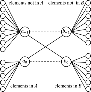
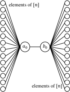
Figure 1: Reductions of Set Disjointness to Distributed Steiner Forest. Left: reduction to dsf-cr (solid edges are light, dashed edges are heavy). Right: reduction to dsf-ic (all edges have unit weight).

This completes the description of the dsf-cr instance. We now claim that if $\mathcal{A}$ computes a $\rho$-approximation to dsf-cr, then we can output the answer “YES” to the original SD instance iff $\mathcal{A}$ produces an output that does not include neither of the heavy edges $\left\{(a_{0},b_{-1}),(a_{-1},b_{0})\right\}$. To see this, consider the optimal solutions. If $A\cap B=\emptyset$, then all connection requests can be satisfied using edges from $E_{A}\cup E_{B}\cup\left\{(a_{0},b_{-1}),(a_{-1},b_{0})\right\}$. Hence the optimal cost is at most $2n+2$, which means that any $\rho$-approximate solution cannot include a heavy edge; and if $A\cap B\neq\emptyset$, then any solution must include at least one of the heavy edges, and hence its weight is larger than $\rho(2n+2)$.

It follows that if $\mathcal{A}$ is a $\rho$-approximate solution to dsf-cr, then the following algorithm solves SD: Alice and Bob construct the graph based on their local input without any communication. Then Alice simulates $\mathcal{A}$ on the $\left\{a_{i}\right\}$ nodes and Bob simulates $\mathcal{A}$ on the $\left\{b_{i}\right\}$ nodes. The only communication required between Alice and Bob to run the simulation is the messages that cross the edges in $E_{AB}$. Now, solving SD requires exchanging $\Omega(n)$ bits in the worst case (see, e.g., [15]). In the $\textsc{congest}(\ell)$ model, at most $\mathcal{O}(\ell)$ bits can cross $E_{AB}$ in a round, and hence it must be the case that the running time of $\mathcal{A}$ is in $\Omega(n/\ell)\subseteq\Omega(t/\ell)$. ∎

Remarks.
$\bullet$ In the lower bound, $n$ is a parameter describing the universe size of the input to SD. Let $n^{\prime}$ denote the number of nodes in the corresponding instance of dsf-cr. Note that we can set $n^{\prime}$ to any number larger than $2n+2$ just by adding isolated nodes. Similarly we can extend the diameter to any number larger than $3$ so long as it’s smaller than $n^{\prime}-2n+1$ by attaching a chain of $n^{\prime}-(2n+2)$ nodes to $a_{1}$. Finally, we can also extend $k$ to any number larger than $2$ by adding pairs of nodes $\left\{(c_{i},c_{i}^{\prime})\right\}$, each pair connected by an edge, and have $R_{c_{i}}=\left\{c_{i}^{\prime}\right\}$.
$\bullet$ Since $D$ is a trivial lower bound, we may apply Lemma 2.3 to convert any dsf-cr instance with $k\geq 2$ into an dsf-ic instance without losing worst-case performance w.r.t. the set of the considered parameters. (If we are guaranteed that $k=1$, the transformation is trivial, as all terminals are to be connected.)
$\bullet$ We note that in the hard instances of SD, $|A|,|B|\in\Theta(n)$ and $|A\cap B|\leq 1$.
$\bullet$ The hardness result applies to dsf-cr algorithms that do not require symmetric requests. More specifically, if the dsf-cr algorithm works only for inputs satisfying $\forall u,v(u\in R_{v}\iff v\in R_{u})$, then the reduction from SD fails.
$\bullet$ The special case of MST ($t=n$ and $k=1$) can be solved in time $\tilde{\mathcal{O}}(\sqrt{n}+D)$ [16].

Proof of Lemma 3.3.

As in Lemma 3.1, we reduce Set Disjointness (SD) to dsf-ic. Specifically, the reduction is as follows. Let $A,B$ be the input sets to Alice and Bob, respectively, where $|A|,|B|\subseteq[n]$. Alice constructs a star whose leaves are the nodes $\left\{a_{i}\right\}_{i=1}^{n}$, all connected to a center node $a_{0}$ (see Figure 1 right). For each node $a_{i}$ Alice sets $\lambda(a_{i})=i$ if $i\in A$ and $\lambda(a_{i})=\bot$ otherwise. Similarly Bob constructs another star whose leaves are $\left\{b_{i}\right\}_{i=1}^{n}$, all connected to the center node $b_{0}$, and sets $\lambda(b_{i})=i$ if $i\in B$ and $\lambda(b_{i})=\bot$ otherwise. In addition the instance to dsf-ic contains the edge $(a_{0},b_{0})$. All edges have unit weight. Note that using dsf-ic terminology, we have that the number of input components satisfies $k\leq n$.

We now claim that given any $\rho$-approximation algorithm $\mathcal{A}$ for dsf-ic, the following algorithm solves SD: Alice and Bob construct the graph (without any communication), and then they simulate $\mathcal{A}$, where Alice simulates all the $\left\{a_{i}\right\}$ nodes and Bob simulates all the $\left\{b_{i}\right\}$ nodes. The answer to SD is YES iff the edge $(a_{0},b_{0})$ is not in the output of $\mathcal{A}$. To show the algorithm correct, consider two cases. If the SD instance is a NO instance, then there exists some $i\in A\cap B$, which implies, by construction, that $a_{i}$ and $b_{i}$ must be connected by the output edges, and, in particular, the edge $(a_{0},b_{0})$ must be in the output of $\cal A$ (otherwise $\cal A$ did not produce a valid output); and if the SD instance was a NO instance, then the optimal solution to the constructed dsf-ic instance contains no edges, i.e., its weight is $0$, and therefore no finite-approximation algorithm may include any edge, and in particular the edge $(a_{0},b_{0})$, in its output. This establishes the correctness of the reduction.

Finally, we note that the simulation of $\mathcal{A}$ requires communicating only the messages that are sent over the edge $(a,b)$. Since, as mentioned above, any algorithm for SD requires communicating $\Omega(n)$ bits between Alice and Bob, we conclude that if $\mathcal{A}$ guarantees finite approximation ratio, the number of bits it must communicate over $(a_{i},b_{i})$ is in $\Omega(n)\subseteq\Omega(k)$, and since in the $\textsc{congest}(\ell)$ model only $\mathcal{O}(\ell)$ bits can be communicated over a single edge in each round, it must be the case that the running time of $\mathcal{A}$ is in $\Omega(k/\ell)$. ∎

Proof of Lemma 3.4.

Follows from the observation that the shortest $s$-$t$ path is a special case of the Steiner Forest problem where $s$ and $t$ are the only two terminals, belonging to the same component. Therefore the lower bound of [8] on distributed algorithms solving the shortest $s$-$t$ path problem applies. ∎

Appendix C Basic Moat Growing Algorithm

input : $\forall v\in V:\lambda(v)\in\Lambda\cup\{\bot\}$ // input components

output : feasible forest $F\subseteq E$ // $2$-approximation

1 $\mathcal{M}_{1}:=\{\{v\}\,|\,v\in T\}$ // moats partition $T$; for $v\in T$, let $M_{i}(v)\in\mathcal{M}_{i}$ s.t. $v\in M_{i}(v)$

2 for each $v\in T$ do

3       $\operatorname{rad}_{0}(v):=0$ // by how much moats grew while $v$’s moat was active

4       $\lambda_{1}(\{v\}):=\lambda(v)$ // input components are merged when moats merge

5       $\operatorname{act}_{1}(\{v\}):=\mathbf{true}$ // satisfied components’ moats become inactive

6$F_{0}:=\emptyset$ // set of selected edges

7 $i:=0$

8 while $\exists M\in\mathcal{M}_{i+1}:\operatorname{act}_{i+1}(M)=\mathbf{true}$ do

9       $i:=i+1$

10       $\mu^{\prime}:=\min_{\mu\in\mathbb{R}^{+}_{0}}\exists v,w\in T:$

11       $~{}~{}\operatorname{act}_{i}(M_{i}(v))=\operatorname{act}_{i}(M_{i}(w))=\mathbf{true}\wedge\operatorname{wd}(v,w)=\operatorname{rad}_{i-1}(v)+\operatorname{rad}_{i-1}(w)+2\mu$

12       $\mu^{\prime\prime}:=\min_{\mu\in\mathbb{R}^{+}_{0}}\exists v,w\in T:$

13       $~{}~{}\operatorname{act}_{i}(M_{i}(v))\neq\operatorname{act}_{i}(M_{i}(w))=\mathbf{false}\wedge\operatorname{wd}(v,w)=\operatorname{rad}_{i-1}(v)+\operatorname{rad}_{i-1}(w)+\mu$

14       $\mu_{i}:=\min\{\mu^{\prime},\mu^{\prime\prime}\}$ // minimal moat growth so that two moats touch

15       for each $u\in T$ with $\operatorname{act}_{i}(M_{i}(u))=\mathbf{true}$ do

16             $\operatorname{rad}_{i}(u):=\operatorname{rad}_{i-1}(u)+\mu_{i}$ // grow moats

17      Denote by $v_{i},w_{i}\in T$ a pair of terminals giving rise to $\mu_{i}$

18       Let $E_{p}$ be the edge set of a least-weight path from $v_{i}$ to $w_{i}$ (drop edges in cycles with $F_{i}$)

19       $F_{i}:=F_{i-1}\cup E_{p}$ // connect $M_{i}(v)$ and $M_{i}(w)$

20       $\mathcal{M}_{i+1}:=\mathcal{M}_{i}\cup\{M_{i}(v_{i})\cup M_{i}(w_{i})\}\setminus\{M_{i}(v_{i}),M_{i}(w_{i})$} // merge moats

21       for each $M\in\mathcal{M}_{i+1}$ do

22             if $M=M_{i}(v_{i})\cup M_{i}(w_{i})$ then

23                   $\lambda_{i+1}(M):=\lambda_{i}(M_{i}(v_{i}))$

24            else if $\lambda_{i}(M)=\lambda(M_{i}(w_{i}))$ then

25                   $\lambda_{i+1}(M):=\lambda_{i}(M_{i}(v_{i}))$ // merge input components (if different)

26            else

27                   $\lambda_{i+1}(M):=\lambda_{i}(M)$

28            

29      if $\{M\in\mathcal{M}_{i+1}\,|\,\lambda_{i+1}(M)=\lambda_{i}(M_{i}(v_{i}))\}=\{M_{i}(v_{i})\cup M_{i}(w_{i})\}$ then

30             $\operatorname{act}_{i+1}(M_{i}(v_{i})\cup M_{i}(w_{i})):=\mathbf{false}$ // new moat’s component connected by $F_{i}$

31      else

32             $\operatorname{act}_{i+1}(M_{i}(v_{i})\cup M_{i}(w_{i})):=\mathbf{true}$

33      for $M\in\mathcal{M}_{i+1}\setminus\{M_{i}(v_{i})\cup M_{i}(w_{i})\}$ do

34             $\operatorname{act}_{i+1}(M):=\operatorname{act}_{i}(M)$

35      

return minimal feasible subset of $F_{i}$ // may have selected useless paths

Algorithm 1 Centralized Moat-Growing.

Definition C.1 (Merges).

Each iteration of the while-loop of Algorithm 1 is called a merge step, or simply a merge. The total number of merges is denoted $i_{\max}$. The number of active moats during the $i^{th}$ merge is denoted $\operatorname{act}_{i}$, i.e., $\operatorname{act}_{i}:=|\{M\in\mathcal{M}_{i}\,|\,\operatorname{act}_{i}(M_{i})=\mathbf{true}\}|$.

Lemma C.2.

For $i\in\{0,\ldots,i_{\max}\}$, the set $F_{i}$ computed by Algorithm 1 is an inclusion-minimal forest such that each $M\in\mathcal{M}_{i+1}$ is the cut of $T$ with a component of $(V,F_{i})$.

Proof.

We show the claim by induction on $i$. We have that $\mathcal{M}_{1}=\{\{v\}\,|\,v\in T\}$ and $F_{0}=\emptyset$, i.e., the claim holds for $i=0$. Now assume that it holds for $i\in\{0,\ldots,i_{\max}\}$ and consider index $i+1$. The choice of $F_{i+1}\setminus F_{i}$ guarantees that the joint moat $M_{i+1}(v_{i+1})\cup M_{i+1}(w_{i+1})$ is subset of the same connectivity component of $(V,F_{i+1})$. To see that no terminal from $T\setminus(M_{i+1}(v_{i+1})\cup M_{i+1}(w_{i+1}))$ is connected to this component by $F_{i+1}$, observe that a least-weight path from $v_{i+1}$ to $w_{i+1}$ contains no terminal from $T\setminus M_{i+1}(v_{i+1})\cup M_{i+1}(w_{i+1})$ (otherwise it is not of least weight or $\mu_{i+1}$ would not have been minimal). By the induction hypothesis, this implies that $M_{i+1}(v_{i+1})\cup M_{i+1}(w_{i+1})$ is a maximal subset of $T$ that is in the same component $(V,F_{i+1})$.

It remains to show that $F_{i+1}$ is an inclusion-minimal forest with this property. Since $F_{i+1}\setminus F_{i}$ closes no cycles, it follows from the induction hypothesis that $F_{i+1}$ is a forest. From this and the inclusion-minimality of $F_{i}$ it follows that deleting any edge from $F_{i}$ will disconnect a pair of terminals in the same moat. Similarly, removing an edge from $F_{i+1}\setminus F_{i}$ will disconnect the new moat $M_{i+1}(v_{i+1})\cup M_{i+1}(w_{i+1})$. ∎

Lemma C.3.

The output $F$ of Algorithm 1 is a feasible forest.

Proof.

By Lemma C.2 and the fact that the algorithm terminates once all moats are inactive, it is sufficient to show that an inactive moat contains only complete input components.

Note that if the algorithm changes component identifiers, it does so by changing them for all moats $M\in\mathcal{M}_{i}$ with $\lambda_{i}(M)=\lambda$ into some $\lambda_{i+1}(M)=\lambda^{\prime}$. Hence all terminals $v\in T$ which initially shared the same value $\lambda(v)$ are always in moats with identical component identifiers. Since initially for each $\lambda\in\Lambda$ there are at least two distinct terminals $v,w\in T$ with $\lambda(v)=\lambda(w)$, for each $\lambda$ initially there are at least two moats $M\in\mathcal{M}_{1}$ with $\lambda_{1}(M)=\lambda$. A merge between moats $M,M^{\prime}\in\mathcal{M}_{i}$ assigns component identifier $\lambda_{i}(M)$ to all moats with identifier $\lambda_{i}(M)$ or $\lambda_{i}(M^{\prime})$. The merged moat (which is a connectivity component of $(T,E_{i})$) becomes inactive if and only if it is the only remaining moat with label $\lambda_{i}(M)$. The statement of the lemma follows. ∎

Lemma C.4.

For any feasible output $F$, Algorithm 1 satisfies that

$$W(F)\geq\sum_{i=1}^{i_{\max}}\operatorname{act}_{i}\mu_{i}.$$

Proof.

We show the statement by induction on $i_{\max}$. The statement is trivial for $i_{\max}=0$ (i.e., no input components), so suppose it holds for $i_{\max}\in\mathbb{N}_{0}$ and consider $i_{\max}+1$. We split up the weight function $W$ into $W_{1}+W_{2}$ so that $W_{1}(F)\geq\operatorname{act}_{1}\mu_{1}$ and define a modified instance to which we can apply the induction hypothesis, proving that $W_{2}(F)\geq\sum_{i=2}^{i_{\max}+1}\operatorname{act}_{i}\mu_{i}$.

For each $e\in E$, define $W_{1}$ to be $W$ within $\bigcup_{v\in T}B_{G}(v,\mu_{1})$ and $0$ outside (boundary edges have the appropriate fraction of their weight) and $W_{2}:=W-W_{1}$. Consider the edge set $F_{C}$ of a connectivity component $C\subseteq T$ induced by $F$. We claim that if it contains $n_{C}\geq 2$ nodes, it must hold that $W_{1}(F_{C})\geq n_{C}\mu_{1}$. To see this, note that the choice of $\mu_{1}$ guarantees that the $B_{\mu_{1}}(v)$ are disjoint for all $v\in T$. Moreover, by definition, any path connecting $v\in T$ to a node outside $B_{\mu_{1}}(v)$ must contain edges of weight at least $\mu_{1}$ within $B_{\mu_{1}}(v)$. The claim follows. Summing over all connectivity components $C\subseteq T$ induced by $F$ (which satisfy $n_{C}\geq 2$ since by the problem definition each terminal must be connected to at least one other terminal), we infer that $W_{1}(F)\geq|T|\mu_{1}=\operatorname{act}_{1}\mu_{1}$.

Recall that $\mathcal{M}_{1}=\{\{v\}\,|\,v\in T\}$. We take the following steps:

• The algorithm replaces the moats $\{v_{1}\}$ and $\{w_{1}\}$ by the joint moat $\{v_{1},w_{1}\}$. For the purpose of our induction, we simply interpret this as setting $T^{\prime}:=T\setminus\{w_{1}\}$ if the resulting moat is active.

• If the merge connected the only two terminals $v_{1}$ and $w_{1}$ sharing the same component identifier, the respective moat becomes inactive. In this case, we also remove $v_{1}$ from $T$, i.e., $T^{\prime}:=T\setminus\{v_{1},w_{1}\}$.

• The algorithm assigns to all moats $M\in\mathcal{M}_{1}$ with $\lambda_{1}(M)=\lambda_{1}(M_{1}(w_{1}))$ the component identifier $\lambda(v_{1})$, i.e., $\lambda_{2}(M):=\lambda_{1}(M_{1}(v_{1}))$. Analogously, we set $\lambda^{\prime}(v):=\lambda(v)$ for all $v\in T^{\prime}\setminus\{v\in T\,|\,\lambda(v)=\lambda(w_{1})\}$ and $\lambda^{\prime}(v):=\lambda(w_{1})$ for $v\in T^{\prime}\cap\{v\in T\,|\,\lambda(v)=\lambda(w_{1})\}$.

• Note that the previous steps guarantee that for each terminal $v\in T^{\prime}$, there is a terminal $v\neq w\in T^{\prime}$ so that $\lambda^{\prime}(v)=\lambda^{\prime}(w)$.

• The new instance of the problem is now given by the graph $G^{\prime}=(V,E,W_{2})$, the terminal set $T^{\prime}$, and the terminal component function $\lambda^{\prime}$.

Consider an execution of Algorithm 1 on the new instance. We make the following observations:

• For each $v\in T$ and any radius $r\in\mathbb{R}^{+}_{0}$, it holds that $B_{G^{\prime}}(v,r)=B_{G}(v,r+\mu_{1})$.

• Since $B_{G^{\prime}}(v_{1},r)=B_{G^{\prime}}(w_{1},r)$ (as their distance in $G^{\prime}$ is $0$), deleting $w_{1}$ from the set of terminals has the same effect as joining them into one moat.

• Hence, if the merged moat $\{v_{1},w_{1}\}$ remains active and thus $v_{1}$ is part of the set of terminals of the new instance, we get a one-to-one correspondence between merges of the two instances, i.e., it holds that $\operatorname{act}_{i+1}=\operatorname{act}_{i}^{\prime}$ and $\mu_{i+1}=\mu_{i}^{\prime}$ for all $i\in\{1,\ldots,i_{\max}\}$ (where ^′ indicates values for the new instance).

• By the induction hypothesis, this implies that

  $$W_{2}(F)\geq\sum_{i=1}^{i_{\max}}\operatorname{act}_{i}^{\prime}\mu_{i}^{\prime}=\sum_{i=2}^{i_{\max}+1}\operatorname{act}_{i}\mu_{i}.$$

• If $\{v_{1},w_{1}\}$ became inactive, but never participates in a merge, the same arguments apply.

Hence, suppose that $\{v_{1},w_{1}\}\in\mathcal{M}_{i_{0}}$ participates in a merge in step $i_{0}$. For all indices $i<i_{0}-1$, the above correspondence holds. Moreover, since $\{v_{1},w_{1}\}$ is inactive, (i) the moat $M\in\mathcal{M}_{i_{0}}$ with which it is merged must satisfy that $\operatorname{act}_{i_{0}}(M)=\mathbf{true}$ and (ii) we have that $\operatorname{act}_{i_{0}+1}(M\cup\{v_{1},w_{1}\})$, i.e., the resulting moat is active (as $\lambda_{i_{0}}(\{v_{1},w_{1}\})=\lambda_{i_{0}}(M^{\prime})$ for any $M^{\prime}\in\mathcal{M}_{i_{0}}$ would contradict the fact that $\{v_{1},w_{1}\}$ is inactive). Thus, the merge does not affect the number of active moats, i.e., $\operatorname{act}_{i_{0}+1}=\operatorname{act}_{i_{0}}$. Furthermore, it holds that $\operatorname{rad}_{i_{0}}(v_{1})=\operatorname{rad}_{i_{0}}(w_{1})=\mu_{1}$, since $\{v_{1},w_{1}\}$ has been active only during merge $1$. We conclude that, for any $r\in\mathbb{R}^{+}_{0}$,

$$\bigcup_{v\in M\cup\{v_{1},w_{1}\}}B_{G}(v,\operatorname{rad}_{i_{0}+1}(v)+r)=\bigcup_{v\in M}B_{G^{\prime}}(v,\operatorname{rad}_{i_{0}-1}^{\prime}(v)+r),$$

as the moats of size $\mu_{1}$ around $v_{1}$ and $w_{1}$ at the end of the $i^{th}$ merge exactly compensate for the fact that the edges inside the respective weighted balls in $G$ have no weight in $G^{\prime}$. By induction on $i\in\{i_{0}+1,\ldots,i_{\max}+1\}$, it follows that, for any $r\in\mathbb{R}^{+}_{0}$,

$$\bigcup_{v\in M\cup\{v_{1},w_{1}\}}B_{G}(v,\operatorname{rad}_{i}^{\prime}(v)+r)=\bigcup_{v\in M}B_{G^{\prime}}(v,\operatorname{rad}_{i-2}^{\prime}(v)+r),$$

and we can map the following merges of the two runs onto each other, i.e., $\mu_{i_{0}}+\mu_{i_{0}+1}=\mu_{i_{0}-1}^{\prime}$ and, for $i\in\{i_{0},\ldots,i_{\max}-1\}$, $\mu_{i+2}=\mu_{i}^{\prime}$ as well as $\operatorname{act}_{i+2}=\operatorname{act}_{i}$. In particular,

$$\operatorname{act}_{i_{0}}\mu_{i_{0}}+\operatorname{act}_{i_{0}+1}\mu_{i_{0}+1}=\operatorname{act}_{i_{0}}(\mu_{i_{0}}+\mu_{i_{0}+1})=\operatorname{act}_{i_{0}-1}^{\prime}\mu_{i_{0}-1}^{\prime},$$

and the induction hypothesis yields that

$$W_{2}(F)\geq\sum_{i=1}^{i_{\max}-1}\operatorname{act}_{i}^{\prime}\mu_{i}^{\prime}=\sum_{i=2}^{i_{\max}+1}\operatorname{act}_{i}\mu_{i}.$$

Hence, in both cases $W(F)=W_{1}(F)+W_{2}(F)\geq\sum_{i=1}^{i_{\max}+1}\operatorname{act}_{i}\mu_{i}$, and the proof is complete. ∎

Proof of Theorem 4.1.

By Lemma C.3, the output $F$ of the algorithm is a feasible forest. With each merge, the algorithm adds the edges of a path of cost $\operatorname{rad}_{i}(v_{i})+\operatorname{rad}_{i}(w_{i})$ to $F$. Hence

$$W(F)\leq\sum_{i=1}^{i_{\max}}\operatorname{rad}_{i}(v_{i})+\operatorname{rad}_{i}(w_{i})\\ =\sum_{i=1}^{i_{\max}}\left(\sum_{\begin{subarray}{c}j=1\\ \operatorname{act}^{(j)}(M_{j}(v_{j}))=\mathbf{true}\end{subarray}}^{i}\mu_{j}+\sum_{\begin{subarray}{c}j=1\\ \operatorname{act}^{(j)}(M_{j}(w_{j}))=\mathbf{true}\end{subarray}}^{i}\mu_{j}\right).$$

We construct $G^{\prime}$ and $F^{\prime}$ from $(V,F\cup F_{i-1})$ by contracting edges in $B_{G}(v,\sum_{j=1}^{i-1}\mu_{j})$ for all $v\in T$. If edges are “partially contracted” since they are only fractionally part of $B_{G}(v,\sum_{j=1}^{i-1}\mu_{j})$ for some $v\in T$, their weight simply is reduced accordingly; note that since $F$ is a forest, no edges are “merged”, i.e., the resulting weights are well-defined. By Lemma C.2, this process identifies for each moat $M\in\mathcal{M}_{i-1}$ its terminals. Note that the edges from $F_{i-1}$ are completely contained in these balls. We interpret the set of active moats $T^{\prime}=\{M\in\mathcal{M}_{i}\,|\,\operatorname{act}_{i}(M)=\mathbf{true}\}$ (which after contraction are singletons) as the set of terminals in $G^{\prime}$. Since $F$ is minimal w.r.t. satisfying all constraints, so is $F^{\prime}$ (where in $G^{\prime}$ two terminals need to be connected if the corresponding moats contain terminals that need to be connected). As only active moats contain terminals with unsatisfied constraints (cf. Lemma C.3), $F^{\prime}$ is the union of at most $|T^{\prime}|-1=\operatorname{act}_{i}-1$ shortest paths between terminal pairs from $T^{\prime}$ that contain no other terminals.

Now consider the balls $B_{G^{\prime}}(v,\mu_{i})$ around nodes $v\in T^{\prime}$. By the choice of $\mu_{i}$, they are disjoint. For each such ball $B_{G^{\prime}}(v,\mu_{i})$, by definition any least-weight path has edges of weight at most $\mu_{i}$ within the ball. We claim that any path in $F^{\prime}$ that connects nodes $v,w\in T^{\prime}$, but contains no third node $u\in T^{\prime}\setminus\{v,w\}$, does not pass through $B_{G^{\prime}}(u,\mu_{i})$ for any $u\in T^{\prime}$. Otherwise, consider the subpath from $v$ to a node in $B_{G^{\prime}}(u,\mu_{i})$ for some $u\in T^{\prime}\setminus\{v,w\}$ and concatenate a shortest path from its endpoint to $u$. The result is a path from $v$ to $u$ that smaller weight than the original path from $v$ to $w$. Symmetrically, there is a path shorter than the one from $v$ to $w$ connecting $w$ and $u$. However, together with the fact that the algorithm connects moats incrementally using least-weight paths of ascending weight implies that the pairs $\{v,u\}$ and $\{w,u\}$ must end up in the same moat before the path connecting $v$ and $w$ is added. By transitivity of connectivity this necessitates that $v$ and $w$ are in the same moat when a path connecting them is added, a contradiction. We conclude that indeed each of the considered paths passes through the balls around its endpoints only.

Overall, we obtain that in the above double summation, for each index $i$, there are at most $2(\operatorname{act}_{i}-1)$ summands of $\mu_{i}$: $2$ for each of the at most $\operatorname{act}_{i}-1$ paths connecting nodes in $T^{\prime}$ considered in the previous paragraph (note that the contraction did not change weights of edges covered by these summands). We conclude that

$$W(F)\leq\sum_{i=1}^{i_{\max}}\left(\sum_{\begin{subarray}{c}j=1\\ \operatorname{act}^{(j)}(M_{j}(v_{j}))=\mathbf{true}\end{subarray}}^{i}\mu_{j}+\sum_{\begin{subarray}{c}j=1\\ \operatorname{act}^{(j)}(M_{j}(w_{j}))=\mathbf{true}\end{subarray}}^{i}\mu_{j}\right)\\ \leq\sum_{i=1}^{i_{\max}}2(\operatorname{act}_{i}-1)\mu_{i}\\ <2\sum_{i=1}^{i_{\max}}\operatorname{act}_{i}\mu_{i}.$$

By Lemma C.4, this is at most twice the cost of any feasible solution. In particular, the cost of $F$ is smaller than twice that of an optimal solution. ∎

Appendix D Rounded Moat Radii

input : $\forall v\in V:\lambda(v)\in\Lambda\cup\{\bot\}$ // input components

output : feasible forest $F\subseteq E$ // $2$-approximation

1 $\mathcal{M}_{1}:=\{\{v\}\,|\,v\in T\}$ // moats partition $T$; for $v\in T$, let $M_{i}(v)\in\mathcal{M}_{i}$ s.t. $v\in M_{i}(v)$

2 for each $v\in T$ do

3       $\operatorname{rad}_{0}(v):=0$ // by how much moats grew while $v$’s moat was active

4       $\lambda_{1}(\{v\}):=\lambda(v)$ // input components are merged when moats merge

5       $\operatorname{act}_{1}(\{v\}):=\mathbf{true}$ // satisfied components’ moats become inactive

6$F_{0}:=\emptyset$ // set of selected edges

7 $i:=0$

8 $\hat{\mu}:=1$

9 while $\exists M\in\mathcal{M}_{i+1}:\operatorname{act}_{i+1}(M)=\mathbf{true}$ do

10       $i:=i+1$

11       $\mu^{\prime}:=\min_{\mu\in\mathbb{R}^{+}_{0}}\exists v,w\in T:$

12       $~{}~{}\operatorname{act}_{i}(M_{i}(v))=\operatorname{act}_{i}(M_{i}(w))=\mathbf{true}\wedge\operatorname{wd}(v,w)=\operatorname{rad}_{i-1}(v)+\operatorname{rad}_{i-1}(w)+2\mu$

13       $\mu^{\prime\prime}:=\min_{\mu\in\mathbb{R}^{+}_{0}}\exists v,w\in T:$

14       $~{}~{}\operatorname{act}_{i}(M_{i}(v))\neq\operatorname{act}_{i}(M_{i}(w))=\mathbf{false}\wedge\operatorname{wd}(v,w)=\operatorname{rad}_{i-1}(v)+\operatorname{rad}_{i-1}(w)+\mu$

15       $\mu_{i}:=\min\{\mu^{\prime},\mu^{\prime\prime}\}$ // minimal moat growth so that two moats touch

16       if $\sum_{j=1}^{i}\mu_{j}\geq\hat{\mu}$ then

17             $\mu_{i}:=\hat{\mu}-\sum_{j=1}^{i-1}\mu_{j}$ // stop moat growth at $\hat{\mu}$

18             $F_{i}:=F_{i-1}$ // no merge, just checking whether moats are active

19             $\mathcal{M}_{i+1}:=\mathcal{M}_{i}$

20             for each $M\in\mathcal{M}_{i}$ do

21                   $\lambda_{i+1}(M):=\lambda_{i}(M)$

22                   if $\{M^{\prime}\in\mathcal{M}_{i}\,|\,\lambda_{i}(M^{\prime})=\lambda_{i}(M)\}=\{M\}$ then

23                         $\operatorname{act}_{i+1}(M):=\mathbf{false}$ // moat’s terminals satisfied

24                  else

25                         $\operatorname{act}_{i+1}(M):=\mathbf{true}$

26                  

27            $\hat{\mu}:=(1+\varepsilon/2)\hat{\mu}$ // threshold for next check

28      else

29             Denote by $v_{i},w_{i}\in T$ a pair of terminals giving rise to $\mu_{i}$

30             Let $E_{p}$ be the edges of a least-weight path from $v_{i}$ to $w_{i}$ (drop edges in cycles with $F_{i}$)

31             $F_{i}:=F_{i-1}\cup E_{p}$ // connect $M_{i}(v)$ and $M_{i}(w)$

32             $\mathcal{M}_{i+1}:=\mathcal{M}_{i}\cup\{M_{i}(v_{i})\cup M_{i}(w_{i})\}\setminus\{M_{i}(v_{i}),M_{i}(w_{i})$} // merge moats

33             $\lambda_{i+1}(M_{i}(v_{i})\cup M_{i}(w_{i})):=\lambda_{i}(M_{i}(v_{i}))$

34             $\operatorname{act}_{i+1}(M_{i}(v_{i})\cup M_{i}(w_{i})):=\mathbf{true}$

35             for each $M\in\mathcal{M}_{i+1}\setminus\{M_{i}(v_{i})\cup M_{i}(w_{i})\}$ do

36                   if $\lambda_{i}(M)=\lambda(M_{i}(w_{i}))$ then

37                         $\lambda_{i+1}(M):=\lambda_{i}(M_{i}(v_{i}))$ // merge input components (if different)

38                  else

39                         $\lambda_{i+1}(M):=\lambda_{i}(M)$

40                  $\operatorname{act}_{i+1}(M):=\operatorname{act}_{i}(M)$

41            

42      for each $u\in T$ with $\operatorname{act}_{i}(M_{i}(u))=\mathbf{true}$ do

43             $\operatorname{rad}_{i}(u):=\operatorname{rad}_{i-1}(u)+\mu_{i}$ // grow moats

44      

return minimal feasible subset of $F_{i}$ // may have selected useless paths

Algorithm 2 Centralized Approximate Moat-Growing with approximation ratio $(2+\varepsilon)$.

Corollary D.1.

For any solution $F$, Algorithm 2 satisfies that

$$\left(1+\frac{\varepsilon}{2}\right)W(F)\geq\sum_{i=1}^{i_{\max}}\operatorname{act}_{i}\mu_{i},$$

where $i_{\max}$ is the final iteration of the while-loop of the algorithm.

Proof.

Denote by $u_{i}$ the number of unsatisfied moats in the $i^{th}$ iteration of the while-loop of Algorithm 2, i.e., the moats which can terminals that need to be connected to terminals in different moats. Analogously to Lemma C.4, we have that

$$W(F)\geq\sum_{i=1}^{i_{\max}}u_{i}\mu_{i}.$$

Now consider a satisfied moat $M_{i}\in\mathcal{M}_{i}$ that is formed in iteration $i-1$ out of two unsatisfied moats; we call such a moat bad. Denote by $j(M_{i})\geq i$ the first iteration in which a moat $\bar{M}\supseteq M$ is unsatisfied or inactive, whichever happens earlier. Since the minimal edge weight is $1$ and $\hat{\mu}$ is increased by factor $1+\varepsilon/2$ whenever the algorithm checks whether to inactivate moats, it holds that $\sum_{k=i}^{j(M_{i})-1}\mu_{k}\leq\varepsilon/2\cdot\sum_{k=1}^{i-1}\mu_{k}$. As an unsatisfied moat can only be created by merging an unsatisfied moat (with a satisfied or unsatisfied moat), there is a sequence of unsatisfied moats $M_{0}\subseteq M_{1}\subseteq\ldots\subseteq M_{i-1}$ such that $M_{i-1}\subset M_{i}$.

We observe that if we pick a different moat $M^{\prime}$ and merge $i^{\prime}$ as above and apply the same construction, the resulting sequence $M_{0}^{\prime}\subseteq\ldots\subseteq M_{i^{\prime}-1}^{\prime}$ must be disjoint from the sequence $M_{0}\subseteq\ldots\subseteq M_{i-1}$, since for each $j\in\{1,\ldots,i_{\max}\}$, the set of moats $\mathcal{M}_{j}$ forms a partition of $T$ and the sequences contain no unsatisfied moats. We conclude that

$$\sum_{i=1}^{i_{\max}}\operatorname{act}_{i}\mu_{i}\leq\sum_{i=1}^{i_{\max}}u_{i}\mu_{i}+\sum_{i=1}^{i_{\max}}\sum_{\begin{subarray}{c}M_{i}\in\mathcal{M}_{i}\\ M_{i}\mbox{ bad}\end{subarray}}\sum_{k=i}^{j(M_{i})-1}\mu_{k}\leq\left(1+\frac{\varepsilon}{2}\right)\sum_{i=1}^{i_{\max}}u_{i}\mu_{i}\leq\left(1+\frac{\varepsilon}{2}\right)W(F).$$

∎

Proof of Theorem 4.2.

Analogous to Theorem 4.1, except that the final bound on the approximation ratio follows from Corollary D.1. ∎

Appendix E Proofs for Section 4.1

Proof of Lemma 4.4.

Clearly, the total number of times moats become inactive is at most $k$, because every input component becomes completely contained in a moat exactly once throughout the execution. When an inactive moat merges, either all its terminals become active again or a new inactive moat is formed. Hence, the total number of merges for which the activity status of some terminals change is at most $2k$. ∎

Proof of Lemma 4.8.

To compute the Voronoi decomposition in phase $j$, we use the single-source Bellman-Ford algorithm, where active moats are sources. All nodes in active moats are initialized with distance $0$, and the edge weights are given by the reduced weight function $\hat{W}_{j}$ (which is known locally, because the moat size is locally known). Messages are tagged by the identifier of the closest source w.r.t. $\hat{W}_{j}$ (the “old” trees are not touched, but simply extended). In $\mathcal{O}(s)$ rounds, the Bellman-Ford algorithm terminates, and the result is that the shortest paths trees are extended to include all nodes in the respective Voronoi regions $\operatorname{Vor}_{j}$ that are not in $\operatorname{Reg}_{j-1}(v)$ for a terminal $v\in T$ with $\operatorname{act}^{(j)}=\mathbf{true}$, and each node knows its distance from the closest moat according to $\hat{W}_{j}$, i.e., $\operatorname{wd}(v,u)-\operatorname{rad}_{i_{j-1}}(v)$. Finally, observe that nodes in $\operatorname{Reg}_{j-1}(v)$ for some $v\in T$ with $\operatorname{act}^{(j)}(v)=\mathbf{false}$ simply can use the information from the previous phase $j-1$. ∎

Lemma E.1.

For each $j\in\{0,\ldots,j_{\max}\}$, it holds that $\bigcup_{v\in T}\operatorname{Reg}_{j}(v)=\bigcup_{v\in T}B_{i_{j}}(v)$.

Proof.

We prove the statement by induction on $j$; it trivially holds for $j=0$, so consider the induction step from $j-1$ to $j$. For any node (or part of an edge) in $\bigcup_{v\in T}\operatorname{Reg}_{j-1}(v)=\bigcup_{v\in T}B_{G}(v,\operatorname{rad}_{i_{j-1}}(v))$, the statement trivially holds by the induction hypothesis. Hence, suppose a node (or part of an edge) is outside $\bigcup_{v\in T}\operatorname{Reg}_{j-1}(v)$ and consider the least-weight path $p$ that leads to $\bigcup_{v\in T,\operatorname{act}^{(j)}(v)=\mathbf{true}}\operatorname{Reg}_{j-1}(v)$ (for simplicity, suppose it contains no fractional edges; the general case follows by subdividing edges into lines). Suppose $v\in T$ is the terminal in whose region $\operatorname{Reg}_{j-1}(v)$ the path ends. Then, by the definition of reduced weights and $\operatorname{Vor}_{j}(v)$, the path is contained in $\operatorname{Vor}_{j}(v)\setminus\bigcup_{v\in T,\operatorname{act}^{(j)}(v)=\mathbf{true}}\operatorname{Reg}_{j-1}(v)$. Hence, if $W(p)\leq\operatorname{rad}_{i_{j}}(v)-\operatorname{rad}_{i_{j-1}}(v)$, i.e., the node (or part of an edge) is contained in $B_{i_{j}}(v)$, it must be in $\bigcup_{v\in T}\operatorname{Reg}_{j}(v)$. The choice of $v$ implies that $p\subseteq B_{i_{j}}(v)$ is equivalent to $p\subseteq\bigcup_{v\in T,\operatorname{act}^{(j)}(v)=\mathbf{true}}B_{i_{j}}(v)$. Because the node (or part of an edge) is outside $\bigcup_{v\in T}\operatorname{Reg}_{j-1}(v)=\bigcup_{v\in T}\operatorname{Reg}_{j}(v)$, this is equivalent to the node (or part of an edge) being in $\bigcup_{v\in T}B_{i_{j}}(v)$. We conclude that $\bigcup_{v\in T}\operatorname{Reg}_{j}(v)=\bigcup_{v\in T}B_{i_{j}}(v)$, i.e., the induction step succeeds. ∎

Proof of Lemma 4.9.

Since $p$ is a least-weight path, $W(p)=\operatorname{wd}(v_{i},w_{i})$. By the definition of $\mu_{i}$, hence $W(p)=\operatorname{rad}_{i}(v_{i})+\operatorname{rad}_{i}(w_{i})$. By Lemma E.1, $\bigcup_{v\in T}\operatorname{Reg}_{j(i)}(v)=\bigcup_{v\in T}B_{i_{j(i)}}(v))$. Thus, any path $q$ between to terminals that enters the uncovered region in phase $j(i)$ must have weight $W(q)>W(p)$; in particular, $p$ cannot enter the uncovered region.

Hence, assume for contradiction that $p$ enters $\operatorname{Reg}_{j(i)}(u)$ for some $u\in T$. Denote by $p^{\prime}$ a minimal prefix of $p$ ending at node $x\in\operatorname{Reg}_{j(i)}(u)$ for some $u\in T$. We make a case distinction, where the first case is that $u\in M_{i}(v_{i})$. Consider the concatenation $q_{1}$ of the suffix of $p$ starting at $x$ to a least-weight path from $u$ to $x$. By the definition of regions, we have that

$$W(q_{1})-\operatorname{rad}_{i_{j(i)-1}}(w_{i})-\operatorname{rad}_{i_{j(i)-1}}(u) = W_{j(i)}(q_{1})$$

$$< W_{j(i)}(p)$$

$$= W(p)-\operatorname{rad}_{i_{j(i)-1}}(w_{i})-\operatorname{rad}_{i_{j(i)-1}}(v_{i}).$$

By assumption $u$ and $v_{i}$ are in the same moat after merge $i-1$, which must have been active. By the definition of merge phases, $u$ and $v_{i}$ thus were both in active moats during all merges $i_{j(i)-1}+1,\ldots,i$. This entails that their $\operatorname{rad}$ variables have been increased by the same value in each of these merges, yielding that

$$W(q_{1})-\operatorname{rad}_{i-1}(w_{i})-\operatorname{rad}_{i-1}(u)<W(p)-\operatorname{rad}_{i-1}(w_{i})-\operatorname{rad}_{i-1}(v_{i}).$$

As $p$ is a least-weight path from $v_{i}$ to $w_{i}$, we conclude that

$$\operatorname{wd}(u,w_{i})-\operatorname{rad}_{i-1}(w_{i})-\operatorname{rad}_{i-1}(u)<\operatorname{wd}(v_{i},w_{i})-\operatorname{rad}_{i-1}(w_{i})-\operatorname{rad}_{i-1}(v_{i}).$$

This contradicts the minimality of $\mu_{i}$, since $u$ is in an active moat in merge $i$.

Hence it must hold $u\notin M_{i}(v_{i})$, which is the second case. Consider the path $q_{2}$ which is the concatenation of a least-weight path between $x$ and $u$ to $p^{\prime}$. Similarly to the first case, we have that

$$W(q_{2})-\operatorname{rad}_{i_{j(i)-1}}(v_{i})-\operatorname{rad}_{i_{j(i)-1}}(u)<W(p)-\operatorname{rad}_{i_{j(i)-1}}(v_{i})-\operatorname{rad}_{i_{j(i)-1}}(w_{i}).$$

If $M_{i}(u)$ is active, $u$ is in active moats during merges $i\in\{i_{j(i)-1}+1,\ldots,i\}$, and similarly to the first case we can infer that

$$\operatorname{wd}(v_{i},u)-\operatorname{rad}_{i-1}(v_{i})-\operatorname{rad}_{i-1}(u)<\operatorname{wd}(v_{i},w_{i})-\operatorname{rad}_{i-1}(v_{i})-\operatorname{rad}_{i-1}(w_{i});$$

the same applies if $\operatorname{act}_{i}(M_{i}(w_{i}))=\mathbf{false}$. Again this contradicts the minimality of $\mu_{i}$, as $M_{i}(v_{i})$ is active.

It remains to consider the possibility that $\operatorname{act}_{i}(M_{i}(u))=\mathbf{false}$ and $\operatorname{act}_{i}(M_{i}(w_{i}))=\mathbf{true}$. Symmetrically to the first case, we can exclude that $u\in M_{i}(w_{i})$. Since $u$ is in inactive moats during phase $j(i)$, it holds that $\operatorname{rad}_{i-1}(u)=\operatorname{rad}_{i_{j(i)-1}}(u)$. By definition of $q_{1}$ and $q_{2}$, we thus have that

$$\operatorname{wd}(v_{i},u)+\operatorname{wd}(w_{i},u)-2\operatorname{rad}_{i-1}(u)\leq W(q_{1})+W(q_{2})-2\operatorname{rad}_{i_{j(i)-1}}(u)<W(p)=\operatorname{wd}(v_{i},w_{i}).$$

As $W(p)=\operatorname{rad}_{i}(v_{i})+\operatorname{rad}_{i}(w_{i})\geq\operatorname{rad}_{i-1}(v_{i})+\operatorname{rad}_{i-1}(w_{i})$, this yields

$$\operatorname{wd}(v_{i},u)+\operatorname{wd}(w_{i},u)-2\operatorname{rad}_{i-1}(u)<2\operatorname{wd}(v_{i},w_{i})-\operatorname{rad}_{i-1}(v_{i})-\operatorname{rad}_{i-1}(w_{i}).$$

By the pidgeon hole principle, we obtain that

$$\operatorname{wd}(v_{i},u)-\operatorname{rad}_{i-1}(u)-\operatorname{rad}_{i-1}(v_{i})<\operatorname{wd}(v_{i},w_{i})-\operatorname{rad}_{i-1}(v_{i})-\operatorname{rad}_{i-1}(w_{i})$$

or that

$$\operatorname{wd}(w_{i},u)-\operatorname{rad}_{i-1}(u)-\operatorname{rad}_{i-1}(w_{i})<\operatorname{wd}(v_{i},w_{i})-\operatorname{rad}_{i-1}(v_{i})-\operatorname{rad}_{i-1}(w_{i}).$$

As both $\operatorname{act}_{i}(M_{i}(v_{i}))=\operatorname{act}_{i}(M_{i}(w_{i}))=\mathbf{true}$ and $u\notin M_{i}(v_{i})\cup M_{i}(w_{i})$, this contradicts the minimality of $\mu_{i}$. We conclude that all cases lead to contradiction and therefore the claim of the lemma is true. ∎

Proof of Lemma 4.14.

To specify the execution of Algorithm 1, the following symmetry breaking rule is introduced: Among all feasible combinations of choices for $v_{i}$ and $w_{i}$ in Line 1, and paths $p$ in Line 2, the algorithm selects the path $p_{v_{i}ew_{i}}$ such that $\{v_{i},w_{i}\}\cup e$ is minimal w.r.t. the order used in point (iii) of Definition 4.12.

For the respective execution, we show the claim by induction on the merges $i$. We anchor the induction at $i=0$, for which $F_{0}=\emptyset$, which equals the union of edges in the paths associated with $\emptyset$. Hence, consider merge $i\in\{1,\ldots,i_{\max}\}$, assuming that the claim holds for the first $i-1$ merges/candidate merges in $F_{c}$. Lemma 4.9 shows that the least-weight path $p_{v_{i}ew_{i}}$ from $v_{i}$ to $w_{i}$ selected by Algorithm 1 in merge $i$ satisfies that $p_{v_{i}ew_{i}}\in\operatorname{Reg}_{j(i)}(v_{i})\cup\operatorname{Reg}_{j(i)}(w_{i})$. Since $\operatorname{act}^{(j(i))}(v_{i})=\mathbf{true}$ and $M_{i_{j(i)}+1}(v_{i})\subseteq M_{i}(v_{i})\neq M_{i}(w_{i})\supseteq M_{i_{j(i)}+1}(w_{i})$, $e$ induces candidate merge $(\{v_{i},w_{i}\},j(i),\hat{W}_{j(i)}(p_{v_{i}ew_{i}}\cap\operatorname{Reg}_{j(i)}(v_{i})),e)$.

We claim that this candidate merge is the next element of $F_{c}$ (according to the order). Assuming otherwise for contradiction, the symmetry breaking rules specified above imply that there is a candidate merge $(\{v,w\},j,\hat{W}_{j}(p_{ve^{\prime}w}\cap\operatorname{Reg}_{j}(v)),e^{\prime})$ which (i) satisfies that $(j,\hat{W}_{j}(p_{ve^{\prime}w}\cap\operatorname{Reg}_{j}(v))<j,\hat{W}_{j}(p_{v_{i}ew_{i}}\cap\operatorname{Reg}_{j}(v))$ (lexicographically), (ii) closes no cycle with the first $i-1$ selected merges, and (iii) satisfies that $\operatorname{act}^{(j)}(v)=\mathbf{true}$. By property (ii) and the induction hypothesis, $M_{i}(v)\neq M_{i}(v)$. If $j^{\prime}<j(i)$, the candidate merge must have been selected as element $i^{\prime}<j(i)\leq i$ into $F_{c}$, contradicting the fact that no w.r.t. $G_{c}$ duplicate edges are selected into $F_{c}$. Therefore, by (i), $j=j(i)$ and $\hat{W}_{j}(p_{ve^{\prime}w}\cap\operatorname{Reg}_{j}(v))<\hat{W}(p_{v_{i}ew_{i}}\cap\operatorname{Reg}_{j}(v_{i}))$. By the definition of regions, this implies that $\operatorname{rad}_{i}(v)+\operatorname{rad}_{i}(w)>\operatorname{wd}(v,w)$. It follows that $v$ and $w$ must satisfy that $M_{i}(v)=M_{i}(w)$, since otherwise Algorithm 1 would merge these moats instead in merge $i$. However, the induction hypothesis and the facts that $F_{c}$ closes no cycles and contains no duplicate edges entail that $M_{i}(v)\neq M_{i}(w)$, a contradiction; the claim follows.

Because the path associated with candidate merge $(\{v_{i},w_{i}\},j(i),\hat{W}_{j(i)}(p_{v_{i}ew_{i}}\cap\operatorname{Reg}_{j(i)}(v_{i})),e)$ is $p_{v_{i}ew_{i}}$, the induction hypothesis yields that the edge set of the union of paths associated with the first $i$ elements of $F_{c}$ is a superset of $F_{i}$. Since $p_{v_{i}ew_{i}}\setminus\{e\}$ is contained in the shortest-path-trees at $v_{i}$ and $w_{i}$, the respective edges close no cycles with the cut of $F_{i-1}$ with the trees rooted at $v_{i}$ and $w_{i}$, respectively. Since $M_{i}(v_{i})\neq M_{i}(w_{i})$, $e$ does not close a cycle in $F_{i}$ either. We conclude that Algorithm 1 adds all edges in $p_{v_{i}ew_{i}}$ to $F_{i-1}$ when $p_{v_{i}ew_{i}}$ does not close a cycle with $F_{i-1}$, implying that constructing $F_{i}$. Hence, the the edge set of the union of paths associated with the first $i$ elements of $F_{c}$ equals $F_{i}$, the induction step succeeds, and the proof is complete. ∎

Sketch of Proof of Lemma 4.14.

We use the edge elimination procedure introduced for MST [11, 16], which works as follows. We use an (unweighted) BFS tree rooted at some node $R\in V$, which can be constructed in $\mathcal{O}(D)$ rounds. For round $r\in\mathbb{N}$, let $F_{u}(r)$ denote the set of candidate merges node $u\in V$ holds at the end of round $r$, where $F_{u}(0):=E_{c}(u)$. In each round each node executes the following convergecast procedure.

1. ${F}_{u}(r-1)$ is scanned in ascending weight order, and a merge that closes a cycle in $G_{c}$ with the union of $F_{c}^{\prime}$ and previous merges is deleted. (This is possible because the merges are tagged by the connectivity components of the terminals they join in $(T,F_{c}^{\prime})$.)

2. The least-weight unannounced merge in $F_{u}(r-1)$ is announced by $u$ to its parent ($R$ skips this step).

3. ${F}_{u}(r)$ is assigned the union of $F_{u}(r-1)$ with all merges received from children.

Once all sets stabilize (which can be detected at an overhead of $\mathcal{O}(D)$ rounds), the set $F_{R}(r)$ equals $\bigcup_{j^{\prime}=1}^{j}F_{c}^{(j^{\prime})}\setminus F_{c}^{\prime}$. Perfect pipelining is achieved, leading to the stated running time bound. ∎

Proof of Lemma 4.16.

Set $F_{c}^{\prime}:=\bigcup_{j^{\prime}=1}^{j-1}F_{c}^{(j^{\prime})}$. Each node $u\in V$ locally computes the connectivity components of $(T,F_{c}^{\prime})$ and tags the elements of $E_{c}(u)$ accordingly. We apply the same procedure as for Lemma 4.14, except that we need to detect termination differently, as we would like to stop the routine once the root knows $F_{c}^{(j)}$. The pipelining guarantees that after $D+i$ rounds of the routine, the first $i$ elements of the ascending list of merges (whose sublist up to element $|F_{c}^{(j)}|$ equals $F_{c}^{(j)}$) are known to the root. Since the root knows $F_{c}^{\prime}$ and, for each $v\in T$, $\lambda(v)$, it can locally compute the variables $\operatorname{act}^{(j)}(v)$, $v\in V$, and will detect in round $D+|F_{c}^{(j)}|$ that some terminal changes its activity status. This enables to determine when to terminate the collection routine and which elements of $F_{R}(D+|F_{c}^{(j)}|)$ constitute $F_{c}^{(j)}$. ∎

We put the pieces of our analysis together to bound the time complexity of our algorithm.

Lemma E.2.

The above algorithm can be implemented such that it runs in $\mathcal{O}(sk+t)$ rounds.

Proof.

Clearly, Step 1 can be executed in $\mathcal{O}(D)$ rounds. Step 2 consists of local computations only. By Lemma 4.13, we have that $F_{c}=F_{c}^{(j_{\max})}$, since at the end of merge phase $j_{\max}$, no active terminals remain. We conclude that the loop in Step 3 of the above algorithm is executed for $j_{\max}$ iterations. By Lemma 4.4, $j_{\max}\leq 2k_{0}$.

We claim that iteration $j\in\{1,\ldots,j_{\max}\}$ of the loop can be executed in $\mathcal{O}(s+|F_{c}^{(j)}|)$ rounds, which we show by induction on $j$. The induction hypothesis is that, after $j-1$ iterations of the loop, the prerequisites of Lemma 4.8 are satisfied for index $j-1$, $\operatorname{rad}^{(j-1)}(v)=\operatorname{rad}_{i_{j-1}}(v)$ for all $v\in T$, and the value of the variable $\operatorname{act}^{(j)}(v)$ is correct for each $v\in T$. This is trivially satisfied for $j=1$ by initialization, hence suppose the hypothesis holds for $j\in\{1,\ldots,j_{\max}-1\}$. Under this assumption, Lemma 4.8 shows that Step 3a can be executed in $\mathcal{O}(s)$ rounds, in the sense that the trees become locally known as stated in the lemma. Clearly, this implies that Step 3b can be executed in one round, by each node $u$ sending $v_{u}$ to each neighbor.

Consider $(\{v_{u},v_{u^{\prime}}\},j,\hat{W},\{u,u^{\prime}\})\in E_{c}(u)$. We have that $\operatorname{act}^{(j)}(v_{u})=\mathbf{true}$. For each entry, we have that $v_{u}\neq v_{u^{\prime}}$ and $\{u,u^{\prime}\}\notin\operatorname{Reg}_{j-1}(v_{u})\cap\operatorname{Reg}_{j-1}(v_{u^{\prime}})$. Thus, if $\{u,u^{\prime}\}\in\operatorname{Reg}_{j}(v_{u})\cap\operatorname{Reg}_{j}(v_{u^{\prime}})$, the hypothesis that $\operatorname{rad}_{i_{j-1}}(v_{u})=\operatorname{rad}^{(j-1)}(v_{u})$ implies that

$$\hat{W}=\operatorname{wd}(v_{u},u)-\operatorname{rad}_{i_{j-1}}(v_{u})+W(\{u,u^{\prime}\}\cap T_{u})=W(p_{v_{u}\{u,u^{\prime}\}v_{u^{\prime}}})-\operatorname{rad}_{i_{j-1}}(v_{u})=\hat{W}_{j}(p_{v_{u}\{u,u^{\prime}\}v_{u^{\prime}}})$$

and $(\{v_{u},v_{u^{\prime}}\},j,\hat{W},\{u,u^{\prime}\})$. Hence, $E_{c}^{(j)}\subseteq\bigcup_{u\in V}E_{c}(u)$ and an entry $(\{v_{u},v_{u^{\prime}}\},j,\hat{W},\{u,u^{\prime}\})\in E_{c}(u)$ is a candidate merge if and only if $\{u,u^{\prime}\}\in\operatorname{Reg}_{j}(v_{u})\cap\operatorname{Reg}_{j}(v_{u^{\prime}})$.

As $\operatorname{act}^{(j)}(v_{u})=\mathbf{true}$, it holds that that $\operatorname{rad}_{i_{j}}(v_{u})-\operatorname{rad}_{i_{j-1}}(v_{u}):=\hat{W}_{\max}$ is identical for all $v_{u}\in T$. We have that

$$W(\{u,u^{\prime}\}\cap T_{u})\subseteq\operatorname{Reg}_{j}(v_{u})\Leftrightarrow\operatorname{wd}(v_{u},u)+W(\{u,u^{\prime}\}\cap T_{u})\leq\operatorname{rad}_{i_{j}}(v_{u})\Leftrightarrow\hat{W}\leq\hat{W}_{\max}.$$

Similarly, if $\operatorname{act}^{(j)}(v_{u^{\prime}})=\mathbf{true}$,

$$W(\{u,u^{\prime}\}\cap T_{u^{\prime}})\subseteq\operatorname{Reg}_{j}(v_{u^{\prime}})\Leftrightarrow\hat{W}\leq\hat{W}_{\max},$$

because $\operatorname{rad}_{i_{j-1}}(v_{u^{\prime}})=\operatorname{rad}^{(j-1)}(v_{u^{\prime}})$. It follows that

$$W(\{u,u^{\prime}\}\cap T_{u})\subseteq\operatorname{Reg}_{j}(v_{u})\Leftrightarrow W(\{u,u^{\prime}\}\cap T_{u^{\prime}})\subseteq\operatorname{Reg}_{j}(v_{u^{\prime}}).$$

On the other hand, if $\operatorname{act}^{(j)}(v_{u^{\prime}})=\mathbf{false}$, the statement $W(\{u,u^{\prime}\}\cap T_{u^{\prime}})\subseteq\operatorname{Reg}_{j}(v_{u^{\prime}})$ is trivially satisfied, because $T_{u^{\prime}}$ spans $\operatorname{Reg}_{j}(v_{u^{\prime}})$. We conclude that $(\{v_{u},v_{u^{\prime}}\},j,\hat{W},\{u,u^{\prime}\})\in E_{c}(u)$ is a candidate merge if and only if $\hat{W}\leq\hat{W}_{\max}$.

Therefore, each false candidate in $\bigcup_{u\in V}E_{c}(u)$ is of larger weight than all candidate merges in $E_{c}^{(j)}$. We conclude that the prerequisites of Corollary 4.16 are satisfied for merge phase $j$, yielding that Step 3c can be executed in $\mathcal{O}(D+|F_{c}^{(j)}|)$ rounds.

Step 3d requires local computation only. We observe that:

• For each $v\in T$, $\operatorname{rad}^{(j)}(v)=\operatorname{rad}_{i_{j}}(v)$, since we established that $\mu^{(j)}=\hat{W}_{\max}=\operatorname{rad}_{i_{j}}(v)-\operatorname{rad}_{i_{j-1}}(v)$ for each $v\in T$ with $\operatorname{act}^{(j)}(v)=\mathbf{true}$.

• By Lemma 4.8, the local information available to the nodes from Step 3a and the $\operatorname{rad}^{(j)}$ variables permit to determine, for each $u\in V$, whether $u\in\operatorname{Reg}_{j}(v_{u})$ and the fraction of its incident edges inside $\operatorname{Reg}_{j}(v_{u})$.

• By Lemma 4.13, $\mathcal{M}^{(j+1)}=\mathcal{M}_{i_{j}+1}$, i.e., the moats at the beginning of merge phase $j+1$.

• The computed variables $\operatorname{act}^{(j+1)}(v)$, $v\in T$, are thus correct.

This establishes the induction hypothesis for index $j+1$. The total time complexity of the $j^{th}$ iteration of the loop in Step 3 is $\mathcal{O}(D+s+|F_{c}^{(j)})|)\subseteq\mathcal{O}(s+|F_{c}^{(j)})|)$, yielding a total of

$$\mathcal{O}\left(\sum_{j=1}^{j_{\max}}s+|F_{c}^{(j)})|\right)=\mathcal{O}\left(j_{\max}s+|F_{c}|\right)\subseteq\mathcal{O}(ks+|T|-1)=\mathcal{O}(ks+t)$$

rounds to complete Step 3.

Step 4 requires local computations only. For Step 5, for an edge $\{x,y\}$ inducing a candidate merge from $F_{\min}$, $x$ and $y$ send a token to their respective parents. Each node receiving a token for the first time forwards it, other tokens will be ignored. Edge $\{x,y\}$ and all edges traversed by a token are selected into $F$. Since the goal is to select for each edge $\{x,y\}$ the edge and the paths from $x$ and $y$ to the roots in their respective trees, this rule ensures that $F$ is computed correctly. Because the shortest-path-trees have depth at most $s$ and there is no congestion, this implementation of Step 4 completes in $\mathcal{O}(s)$ rounds (where termination is detected in $\mathcal{O}(D)\subseteq\mathcal{O}(s)$ rounds over the BFS tree). Since Step 6 requires no communication, summing up the time complexities for Steps 1 to 6 yields a total running time bound of $\mathcal{O}(D+t+ks+t+s)=\mathcal{O}(ks+t)$. ∎

Proof of Theorem 4.17.

By Lemma E.2, the above algorithm can be executed within the stated running time bound. By Lemma 4.13, the edge set $F^{\prime}$ of the union of paths associated with $F_{c}$ equals the set $F_{i_{\max}}$ computed by some execution of Algorithm 1. Hence, if we can show that the set $F$ returned in Step 6 of the above algorithm is the minimal subset of $F^{\prime}$ that solves the instance, the theorem readily follows from Theorem 4.1.

Recall that because Algorithm 1 never closes a cycle, $F^{\prime}=F_{i_{\max}}$ is a forest, and so is $F$. By the minimality of $F_{\min}$, any two terminals connected by $F_{\min}$ (viewed as forest in $G_{c}$) must be connected by any subforest of $F^{\prime}$ that is a solution. For any edge $\{x,y\}\in F$, there is an element of $(\{v,w\},\cdot,\cdot,\cdot)\in F_{\min}$ such that $\{x,y\}$ is on the associated path connecting $v$ and $w$. Deleting $\{x,y\}$ from $F$ will disconnect $v$ and $w$ (because $F$ is a forest), implying that the resulting edge set does not solve the instance of dsf-ic. We conclude that $F$ is indeed the edge set returned by Algorithm 1, and therefore optimal up to factor $2$. ∎

E.1 The distributed algorithm

1. Construct a directed BFS tree, rooted at $R$. For each $v\in T$, broadcast $(v,\lambda(v))$ to all nodes (via the BFS tree).

2. Set $j:=1$ (index of the merge phase) and $M_{1}:=\{\{v\}\,|\,v\in T\}$. For each $v\in T$, set $\operatorname{rad}^{(0)}(v):=0$, $\operatorname{act}_{1}(v):=\mathbf{true}$, and $\operatorname{Reg}_{0}(v):=\{v\}$.

3. While $\exists v\in T$ with $\operatorname{act}^{(j)}(v)=\mathbf{true}$:

   1. Compute the collection of shortest-path-trees spanning for each $v\in T$ with $\operatorname{act}^{(j)}=\mathbf{false}$ $\operatorname{Reg}_{j}(v)$ and for each $v\in T$ with $\operatorname{act}^{(j)}=\mathbf{true}$ $\operatorname{Reg}_{j-1}(v)\cup(\operatorname{Vor}_{j}(v)\setminus\bigcup_{w\in T}B_{i_{j-1}}(w))$.

   2. For each $u\in V$, denote by $v_{u}$ the root of the tree ${\cal T}_{u}$ it participates in. For each $u\in V$ with $\operatorname{act}^{(j)}(v_{u})=\mathbf{true}$, locally construct $E_{c}(u)$ as follows. For each neighbor $u^{\prime}$ of $u$ so that $v_{u^{\prime}}\neq v_{u}$ and $\{u,u^{\prime}\}\notin\operatorname{Reg}_{j-1}(v_{u})\cup\operatorname{Reg}_{j-1}(v_{u^{\prime}})$, $u$ adds $(\{v_{u},v_{u^{\prime}}\},j,\operatorname{wd}(v_{u},u)-\operatorname{rad}^{(j-1)}(v_{u})+W(\{u,u^{\prime}\}\cap{\cal T}_{u}),\{u,u^{\prime}\})$ to $E_{c}(u)$. For all other nodes $u$, $E_{c}(u):=\emptyset$.

   3. Determine $F_{c}^{(j)}$ and make it known to all nodes.

   4. Suppose the maximal merge in $F_{c}^{(j)}$ is $(\cdot,\cdot,\mu^{(j)},\cdot)$. Each $u\in V$ locally computes:

      • for $v\in T$ with $\operatorname{act}^{(j)}(v)=\mathbf{true}$, $\operatorname{rad}^{(j)}(v):=\operatorname{rad}^{(j-1)}(v)+\mu^{(j)}$;

      • for $v\in T$ with $\operatorname{act}^{(j)}(v)=\mathbf{false}$, $\operatorname{rad}^{(j)}(v):=\operatorname{rad}^{(j-1)}(v)$;

      • whether $u\in\operatorname{Reg}_{j}(v_{u})$ or not, and the fraction of its incident edges inside $\operatorname{Reg}_{j}(v_{u})$;

      • the set $\mathcal{M}^{(j+1)}$ of connectivity components of the forest on $T$ induced by $\bigcup_{j^{\prime}=1}^{j}F_{c}^{(j)}$ (for $v\in T$, denote by $M_{v}\in\mathcal{M}^{(j+1)}$ the moat so that $v\in M_{v}$);

      • for $v\in T$ with $\exists w\in M_{v},w^{\prime}\in T\setminus M_{v}:\,\lambda(w)=\lambda(w^{\prime})$, $\operatorname{act}^{(j+1)}(v):=\mathbf{true}$;

      • for $v\in T$ with $\nexists w\in M_{v},w^{\prime}\in T\setminus M_{v}:\,\lambda(w)=\lambda(w^{\prime})$, $\operatorname{act}^{(j+1)}(v):=\mathbf{false}$.

   5. $j:=j+1$.

4. Set $F_{c}:=\bigcup_{j^{\prime}=1}^{j-1}F_{c}^{(j)}$. Each node locally computes the minimal subset $F_{\min}\subseteq F_{c}$ such that the induced forest on $T$ connects for each $\lambda\in\Lambda$ all terminals $v\in T$ with $\lambda(v)=\lambda$.

5. $F:=\emptyset$. For each element of $F_{\min}$, suppose $e=\{x,y\}$ is the inducing edge and $p_{vew}$ the associated path. Add $e$ to $F$ and also all edges on the paths from $x$ to $w$ and $y$ to $w$ that are given by the shortest-path-trees spanning $\operatorname{Reg}_{j-1}(v)$ and $\operatorname{Reg}_{j-1}(w)$, respectively.

6. Return $F$.

Appendix F Material for Section 4.2

F.1 Specification of the Algorithm

Specification of the algorithm.

1. Construct a directed BFS tree, rooted at $R$.

2. Set $j:=0$ (index of the merge phase), $F:=\emptyset$, and $\hat{\mu}:=1$. At each $v\in T$, set $\operatorname{rad}^{(0)}(v):=0$, $\operatorname{act}_{1}(v):=\mathbf{true}$, $\operatorname{Reg}_{0}(v):=\{v\}$, $M_{v}:=\{v\}$, and $L(M_{v}):=v$ (the leader of moat $M_{v}$).

3. While $\exists v\in T:\,\operatorname{act}^{(j+1)}(v)=\mathbf{true}$:

   1. While $\sum_{j^{\prime}=1}^{j-1}\mu^{(j^{\prime})}<\hat{\mu}$:

      1. $j:=j+1$.

      2. Compute the shortest-path-trees spanning for each $v\in T$ with $\operatorname{act}^{(j)}=\mathbf{false}$ $\operatorname{Reg}_{j}(v)$ and for other terminals $\operatorname{Reg}_{j-1}(v)\cup(\operatorname{Vor}_{j}(v)\setminus\bigcup_{w\in T}B_{i_{j-1}}(w))$.

      3. For each $u\in V$, denote by $v_{u}$ the root of the tree ${\cal T}_{u}$ it participates in. For each $u\in V$ with $\operatorname{act}^{(j)}(v_{u})=\mathbf{true}$, check whether there is a neighbor $u^{\prime}\in V$ with $\operatorname{act}^{(j)}(v_{u^{\prime}})=\mathbf{false}$. If so, set

         $$c_{u}:=\operatorname*{argmin}\limits_{\begin{subarray}{c}\{u,u^{\prime}\}\in E\\ \operatorname{act}^{(j)}(v_{u^{\prime}})=\mathbf{false}\end{subarray}}\{(\{v_{u},v_{u^{\prime}}\},j,\operatorname{wd}(v_{u},u)-\operatorname{rad}^{(j-1)}(v_{u})+W(\{u,u^{\prime}\}\cap{\cal T}_{u}),\{u,u^{\prime}\})\},$$

         i.e., $c_{u}$ is the least-weight candidate merge with an inactive terminal induced by an edge incident to $u$. For all other nodes $u$, $c_{u}:=\bot$.

      4. Over the BFS tree, determine $(\{v_{c},w_{c}\},j,\hat{W},\{u,u^{\prime}\}):=\operatorname*{argmin}_{u\in V}\{c_{u}\}$ and make it known to all nodes. If there is no such candidate merge or $\hat{W}+\sum_{j^{\prime}=1}^{j-1}\mu^{(j^{\prime})}>\hat{\mu}$, set $\mu^{(j)}:=\hat{\mu}-\sum_{j^{\prime}=1}^{j-1}\mu^{(j^{\prime})}$. Otherwise, $\mu^{(j)}:=\hat{W}$. All terminals $v\in T$ with $\operatorname{act}^{(j)}(v)=\mathbf{true}$ set $\operatorname{rad}^{(j)}(v):=\operatorname{rad}^{(j-1)}(v)+\mu^{(j)}$. Other terminals set $\operatorname{rad}^{(j)}(v):=\operatorname{rad}^{(j-1)}(v)$. Each terminal $v\in T$ broadcasts $\operatorname{rad}^{(j)}(v)-\operatorname{rad}^{(j-1)}(v)$ over its current shortest-path-tree. Each node $u\in V$ determines whether it is in $\operatorname{Reg}_{j}(u_{v})$ and the fraction of its incident edges in $\operatorname{Reg}_{j}(u_{v})$.

      5. If $\mu^{(j)}=\hat{W}$ (i.e., merge phase $j$ does not end the growth phase), terminal $w_{c}$ (i.e., the one with $\operatorname{act}^{(j)}(w_{c})=\mathbf{false}$) broadcasts $L(M_{w})$ over the BFS tree. All terminals $v$ with $L(M_{v})=L(M_{w_{c}})$ set $\operatorname{act}^{(j+1)}(v):=\mathbf{true}$. Each terminal $v\in T$ broadcasts $\operatorname{act}^{(j+1)}(v)$ over its current shortest-path-tree.

   2. For $\lceil\log\sqrt{\min\{t/s,n\}}\rceil$ iterations:

      1. Denote by $\mathcal{M}:=\{\{v\in T\,|\,L(M_{v})=L\}\,|\,\exists w\in T:\,L=L(M_{w})\}$ the set of current moats. Each small moat $M\in\mathcal{M}$ finds the smallest candidate merge $(\{v,w\},j^{\prime},\hat{W},e)$ satisfying that $j^{\prime}\leq j$, $v\in M$, and $w\notin M$ (if there is any). Denote the set of such candidate merges by $F_{C}$.

      2. Interpret $F_{C}$ as the edge set of a simple graph on the node set $\mathcal{M}$, by reading each candidate merge $(\{v,w\},j,\hat{W},e)\in F_{C}$ as an edge $\{M_{v},M_{w}\}$. Define $F_{C}^{\prime}:=\{(\{v,w\},j,\hat{W},e)\in F_{C}\,|\,\mbox{$M_{v}$ and $M_{w}$ are small}\}$. Determine an inclusion-maximal matching $M\subseteq F_{C}^{\prime}\subseteq F_{C}$. Each (small) moat that is not incident to an edge in $M$, but added an edge to $F_{C}$, adds the respective edge to $M$ again, resulting in a set of candidate merges $F_{+}\subseteq F_{C}$.

      3. For each $(\{v,w\},j,\hat{W},e)\in F_{+}$, add the edges of $p_{vew}$ to $F$.

      4. Denote by ${\cal C}$ the set of connectivity components of $(V,F)$. For each $v\in T$, set $M_{v}:=T\cap C_{v}$, where $C_{v}\in{\cal C}$ is the component such that $v\in C$. Each terminal $v\in T$ learns the identifier of $L(M_{v})$, the terminal with largest identifier among all terminals $w$ with $M_{w}=M_{v}$. Each terminal $v\in T$ learns whether $M_{v}$ is small.

      5. For each small $M_{v}$, make the complete set $M_{v}$ known to all its terminals.

   3. For each $v\in T$, broadcast $L(M_{v})$ to all nodes in $\operatorname{Reg}_{j}(v)$ (over its shortest-path-tree).

   4. For each $u\in V$, locally construct $E_{c}(u)$ as follows. Starting from $E_{c}(u):=\emptyset$, for each $j^{\prime}\in\{1,\ldots,j\}$ with $\operatorname{act}_{j^{\prime}}(v_{u})=\mathbf{true}$ and each neighbor $u^{\prime}$ of $u$ so that $v_{u^{\prime}}\neq v_{u}$ and $\{u,u^{\prime}\}\notin\operatorname{Reg}_{j^{\prime}-1}(v_{u})\cup\operatorname{Reg}_{j^{\prime}-1}(v_{u^{\prime}})$, $u$ adds $(\{v_{u},v_{u^{\prime}}\},j^{\prime},\operatorname{wd}(v_{u},u)-\operatorname{rad}^{(j^{\prime}-1)}(v_{u})+W(\{u,u^{\prime}\}\cap\operatorname{Reg}_{j^{\prime}}(v_{u})),\{u,u^{\prime}\})$ to $E_{c}(u)$. Each candidate merge is tagged by the identifiers of the moat leaders $L(M_{v_{u}})$ and $L(M_{v_{u^{\prime}}})$.

   5. Denote by $F_{c}^{\prime}$ the set of candidate merges whose associated paths’ edges have been added to $F$ so far. Determine $F_{+}:=\bigcup_{j^{\prime}=1}^{j}F_{c}^{(j^{\prime})}\setminus F_{c}^{\prime}$.

   6. For each $(\{v,w\},j,\hat{W},e)\in F_{+}$, add the edges of $p_{vew}$ to $F$.

   7. Denote by ${\cal C}$ the set of connectivity components of $(V,F)$. For each $v\in T$, set $M_{v}:=T\cap C_{v}$, where $C_{v}\in{\cal C}$ is the component such that $v\in C$. Each terminal $v\in T$ learns the identifier of $L(M_{v})$, the terminal with largest identifier among all terminals $w$ with $M_{w}=M_{v}$. Each terminal $v\in T$ learns whether $M_{v}$ is small.

   8. For each small $M_{v}$, make the complete set $M_{v}$ known to all its terminals.

   9. For each $v\in T$, determine whether there are $w\in M_{v}$ and $u\in T\setminus M_{v}$ so that $\lambda(w)=\lambda(u)$. If this is the case, set $\operatorname{act}^{(j+1)}(v):=\mathbf{true}$, otherwise set $\operatorname{act}^{(j+1)}(v):=\mathbf{false}$.

4. Return $F$.

F.2 Proofs

Lemma F.1.

For $\varepsilon\in\mathcal{O}(1)$ and any execution of Algorithm 2, there are at most $\mathcal{O}(\log n/\varepsilon)$ growth phases and $\sum_{g=1}^{g_{\max}}k_{g}\in k+\mathcal{O}(\log n/\varepsilon)$.

Proof.

We claim that $\sum_{i=1}^{i_{\max}}\mu_{i}\leq\operatorname{WD}/2$. Assuming the contrary, there must be some active moat $M\in\mathcal{M}_{i_{\max}-1}$. Since the moat is active, there are terminals $v\in M$ and $w\in T\setminus M$ so that $\lambda(v)=\lambda(w)$. Clearly, these terminals were not in the same moats after any merge $i<i_{\max}$ and therefore remain active throughout the entire execution of the algorithm. It follows that $\operatorname{rad}_{v}(i_{\max})=\operatorname{rad}_{w}(i_{\max})=\sum_{i=1}^{i_{\max}}\mu_{i}>\operatorname{WD}/2$. However, by definition $\operatorname{wd}(v,w)\leq\operatorname{WD}$, implying that

$$2\mu_{i_{\max}}\leq\operatorname{wd}(v,w)-\operatorname{rad}_{i_{\max}-1}(v)-\operatorname{rad}_{i_{\max}-1}(w)\leq\operatorname{WD}-\operatorname{rad}_{i_{\max}-1}(v)-\operatorname{rad}_{i_{\max}-1}(w).$$

Because $\mu_{i_{\max}}=\operatorname{rad}_{i_{\max}}(v)-\operatorname{rad}_{i_{\max}-1}(v)=\operatorname{rad}_{i_{\max}}(w)-\operatorname{rad}_{i_{\max}-1}(w)$, this yields the contradiction

$$0\leq\operatorname{WD}-\operatorname{rad}_{i_{\max}}(v)-\operatorname{rad}_{i_{\max}}(w)<0.$$

We conclude that indeed $\sum_{i=1}^{i_{\max}}\mu_{i}\leq\operatorname{WD}/2$. Since $\hat{\mu}$ is initialized to $1$ and grows by factor $1+\varepsilon/2$ with each growth phase, we obtain that the number of growth phases is bounded by

$$1+\left\lceil\log_{1+\varepsilon/2}\left(\frac{\operatorname{WD}}{2}\right)\right\rceil\leq 1+\left\lceil\frac{\log\operatorname{WD}}{\log(1+\varepsilon/2)}\right\rceil\in\mathcal{O}(\log n/\varepsilon),$$

where the last step exploits that for $\varepsilon\in\mathcal{O}(1)$, $\log(1+\varepsilon)\in\Omega(\varepsilon)$. The bound on the number of merge phases follows from this bound and the definition of the $k_{g}$, since there are at most $k$ merges which may result in inactive moats (i.e., input components become satisfied), each of which can be merged only once. ∎

Lemma F.2.

At any stage of the above algorithm, the number of large moats is bounded by $\sigma$ and the connectivity component of $(V,F)$ of a small moat has a hop diameter of at most $\sigma$.

Proof.

The bound on the hop diameter of small moats’ components trivially follows from the fact that they contain at most $\sigma$ nodes.

Suppose $st<n$. We claim that the connectivity component of a moat with $\tau$ terminals contains at most $1+(\tau-1)(s-1)$ nodes. This holds trivially for the initial moats. Now suppose moats $M$ and $M^{\prime}$ are merged. The merging path has at most $s$ hops, implying that at most $s-2$ nodes are added. Hence the new moat has at most $2+(|M\cap T|+|M^{\prime}\cap T|-2)(s-1)+(s-2)\leq 1+(|(M\cup M^{\prime})\cap T|-1)(s-1)$ nodes. The claim follows. This entails that the total number of nodes in moats’ components is bounded by $st$.

We conclude that there are at most $\sigma^{2}$ nodes in moats’ connectivity components w.r.t. $F$, and therefore at most $\sigma$ large moats. ∎

Lemma F.3.

Suppose that after $g-1\in\{0,\ldots,g_{\max}-1\}$ growth phases, the variables $\operatorname{act}^{(j_{g}+1)}(v)$, $\operatorname{rad}^{(j_{g})}(v)=\operatorname{rad}_{i_{j_{g}}}(v)$, the local representations of $\operatorname{Reg}_{j}(v)$, $j\in\{1,\ldots,j_{g}\}$, and the trees spanning them, membership of edges in $F=F_{i_{j_{g}}}$, and $M_{v}=M_{i_{j_{g}}+1}(v)$ are identical to the corresponding values for an execution of Algorithm 2. Then in growth phase $g$, Step 3a of the algorithm correctly computes the terminal decompositions $j\in\{j_{g}+1,\ldots,j_{g+1}\}$, as well as the variables $\operatorname{rad}^{(j)}(v)=\operatorname{rad}_{i_{j}}(v)$ and $\operatorname{act}^{(j+1)}(v)$. It can be completed in $\mathcal{O}(sk_{g})$ rounds.

Proof.

We prove the claim by induction on the iterations $j\in\{j_{g}+1,\ldots,j_{g+1}\}$ of the loop in Step 3a, anchored at $j=j_{g}$. The hypothesis is that all respective values for index $j$ are correct, which holds for $j=j_{g}$ by assumption. For the induction step from $j-1$ to $j$, observe that the hypothesis and Lemma 4.8 yield that Step 3aii can be performed in $\mathcal{O}(s)$ rounds. Clearly, Step 3aiii requires one round of communication only.

If $c_{\min}:=\operatorname*{argmin}_{u\in V}\{c_{u}\}\neq\bot$, suppose $c_{\min}=(\{v,w\},j,\hat{W},e)$. If $\hat{W}+\sum_{j^{\prime}=1}^{j-1}\mu^{(j^{\prime})}\leq\hat{\mu}$, we claim that $c_{\min}\in F^{(j)}$ is the candidate merge completing merge phase $j$. Otherwise (also if $c_{\min}=\bot$), $j=j_{g+1}$ and active moats grow by exactly $\hat{\mu}-\sum_{j^{\prime}=1}^{j-1}\mu^{(j^{\prime})}$ during the merge phase. To see this, recall that merge phase $j$ ends if (i) an active and an inactive moat merge or (ii) active moats have grown by $\hat{\mu}-\sum_{j^{\prime}=1}^{j-1}\mu^{(j^{\prime})}$. Note that, by Lemma 4.8 and the induction hypothesis,

$$\hat{W}_{j}(p_{v_{u}\{u,u^{\prime}\}v_{u^{\prime}}}\cap\operatorname{Reg}_{j}(v_{u}))=\operatorname{wd}(v_{u},u)-\operatorname{rad}^{(j-1)}(v_{u})+W(\cap\{u,u^{\prime}\}\cap T_{u})$$

for any $\{u,u^{\prime}\}\in\operatorname{Reg}_{j-1}(v_{u})\cup(\operatorname{Vor}_{j}(v_{u})\setminus\bigcup_{w\in T}B_{i_{j-1}}(w))\cup\operatorname{Reg}_{j}(v_{u^{\prime}})$ so that $\operatorname{act}^{(j)}(v_{u})=\mathbf{true}$ and $\operatorname{act}^{(j)}(v_{u^{\prime}})=\mathbf{false}$. Moreover, $\{u,u^{\prime}\}\notin\operatorname{Reg}_{j-1}(v_{u})\cup\operatorname{Reg}_{j-1}(v_{u^{\prime}})$, as otherwise $v_{u}$ and $v_{u^{\prime}}$ would have been connected in an earlier merge phase and cannot satisfy that $\operatorname{act}^{(j)}(v_{u})\neq\operatorname{act}^{(j)}(v_{u^{\prime}})$.

Suppose (i) applies, i.e., Algorithm 2 merges the moats of terminals $v_{i_{j}}$ and $w_{i_{j}}$ in step $i_{j}$, and suppose it does so by the path $p_{v_{i_{j}}ew_{i_{j}}}$ induced by $e=\{u,u^{\prime}\}$ with $u\in\operatorname{Reg}_{j}(v_{i_{j}})$ and $u^{\prime}\in\operatorname{Reg}_{j}(w_{i_{j}})$ (by Lemma 4.9, we know that such an edge exists). Since the merge phase ends due to this merge and terminals can become inactive only at the end of a growth phase, it must hold that $\mathbf{true}=\operatorname{act}_{i_{j}}(v_{i_{j}})\neq\operatorname{act}_{i_{j}}(w_{i_{j}})$. It follows that $c_{u}=c_{\min}$, as any $c_{u^{\prime\prime}}<c_{u}$ would imply that another pair of terminals from active and inactive moats would be merged earlier, ending the merge phase at an earlier point. The same argument yields that in case of (ii), no $c_{u}=(\cdot,j,\hat{W},\cdot)$ can exist with $\hat{W}+\sum_{j^{\prime}=1}^{j-1}\mu^{(j^{\prime})}\leq\hat{\mu}$, as otherwise an active and inactive terminal would get merged before the growth phase ends.

We conclude that the above claim holds. It follows that in Step 3aiv, which can be completed in $\mathcal{O}(D+s)=\mathcal{O}(s)$ rounds, the correct variables $\operatorname{rad}^{(j)}(v)$, $v\in T$, and therefore also regions $\operatorname{Reg}_{j}(v)$ are determined. If $j=j_{g+1}$, the induction halts. Otherwise, we know that the merge $i_{j}$ connects an active and inactive moat. Because the input labels of terminals in the inactive moat must be disjoint from those of other terminals (as by the hypothesis the variables $\operatorname{act}^{(j)}$ have correct values), the resulting moat must consist of active terminals; no terminals outside the new moat change their activity status. By the prerequisites of the lemma, the terminals in the inactive moat $M$ recognize their membership by the identifier of their leader $L(M)$. Since any merge with an inactive moat makes its terminals active and no terminals can become inactive except for the end of a growth phase, we conclude that Step 3av results in the correct values of the variables $\operatorname{act}^{(j+1)}(v)$, $v\in T$. Step 3av requires $\mathcal{O}(D+s)=\mathcal{O}(s)$ rounds, resulting in a total complexity of $\mathcal{O}(s)$ of the iteration of the while-loop in Step 3a.

The above establishes that, unless $j=j_{g+1}$, the induction hypothesis is established for index $j+1$. Hence, the induction succeeds. We conclude that there are $k_{g}=j_{g+1}-j_{g}$ iterations of the loop in Step 3a, for each of which we observed that it can be implemented with running time $\mathcal{O}(s)$. ∎

Lemma F.4.

Suppose that the prerequisites of Lemma F.3 are satisfied for growth phase $g$. Then, each candidate merge selected by the above algorithm in Step 3b of growth phase $g$ is in $F_{c}$ for a (specific, for all applications of the lemma to an instance fixed) execution of Algorithm 2. The step can be completed in $\tilde{\mathcal{O}}(\sigma+s)$ rounds.

Proof.

As in Lemma 4.13, we consider the execution of Algorithm 2 employing the same tie breaking mechanism as we use to order candidate merges.

We prove the claim by induction on the iterations of the loop in Step 3b. The hypothesis is that all merges performed by the algorithm up to the beginning of the current loop iteration correspond indeed to candidate merges from $F_{c}$ and the moats $\mathcal{M}$ defined in Step 3bi implicitly given by the variable $L(M_{v})$ known to each $v\in T$ are the moats induced by the union of edges of associated paths. The induction is anchored by the assumptions of the lemma; hence consider some iteration of the loop.

Suppose for a moat $M\in\mathcal{M}$, the smallest candidate merge is $(\{v,w\},j,\hat{W},e)$. By Lemma F.3, the nodes in $e$ can detect the existence of the candidate merge by communicating over $e$; performing this concurrently for all nodes, this takes one round, since each edge induces one candidate merge only. Since the moat is small, by Lemma F.2, the moat’s component in $(V,F)$ has diameter at most $\sigma$. Hence, a spanning tree rooted at the leader can be constructed and used to determine the least-weight candidate merge as specified in Step 2bi within $\mathcal{O}(\sigma+s)$ rounds (the additive $s$ accounts for the depth of the trees of the terminal decomposition).

In Step 2bii, only small moats $M\in\mathcal{M}$ need to participate in the computation. We interpret the subgraph of the graph specified in Step 2bii induced by $F_{C}$ as a directed graph, where each small moat has one outgoing edge. We $3$-color the graph by simulating the Cole-Vishkin algorithm [6] on this graph, where moat leaders take the role of the nodes and communication is routed through the spanning trees of the moats. Observe that since nodes need to receive messages only from their “parent” and send identical messages to their children, the congestion is constant. Hence, each round of the Cole-Vishkin algorithm can be simulated in $\mathcal{O}(\sigma+s)$ rounds in $G$, the depth bound for the trees constructed in Step 2bi. After $\mathcal{O}(\log^{*}|\mathcal{M}|)\in\tilde{\mathcal{O}}(1)$ rounds, a $3$-coloring is computed, which in $3$ additional simulated rounds can be used to determine a maximal matching. After another simulated round, each moat leader in a small moat knows its incident edges from $F_{C}$. Consequently, Step 2biii requires another $\mathcal{O}(\sigma+s)$ rounds.

Concerning Step 3biv, observe that the construction of $F_{+}$ ensures for each connectivity component of $(\mathcal{M},F_{+})$, either all moats in the component are small and it consists of two stars connected by a matching edge, or it is a star centered at a large moat, whose leaves are all small moats. If the former applies, Lemma F.2 shows that Step 3biv can be completed for small moats within $\mathcal{O}(\sigma+s)$ rounds using the edges from $F$ in the respective component of $(V,F)$ only. Moreover, in this time a spanning tree can be constructed and used to count the number of terminals or nodes, respectively, determining whether the new moat is small. For the case where a large moat is involved, the new leader will be the leader of the unique large moat in the respective connectivity component of $(V,F)$. Since this leader is already known to all terminals in the large moat, Lemma F.2 shows that its identifier can be distributed to all nodes in the “attached” small moats in $\mathcal{O}(\sigma+s)$ rounds. Trivially, the resulting moat is large.

With respect to Step 3bv, we again apply Lemma F.2, showing that for each small moat, in $\mathcal{O}(\sigma)$ rounds, a spanning tree with edges from $F$ can be constructed that spans its component in $(V,F)$. This tree is used to broadcast the terminal identifiers of its at most $\sqrt{\min\{st,n\}}$ terminals to all constituent nodes within $\mathcal{O}(\sigma)$ rounds.

To complete the induction step, it thus remains to show that $F_{+}\subseteq F_{c}$ and therefore indeed all edges selected into $F$ in Step 3biii are also selected by the execution of Algorithm 2 that selects the same merges and the associated paths, and also that the computed moats are indeed the cuts of $T$ with the connectivity components of $(V,F)$. Observe that for a candidate merge added to $F_{C}$ by moat $M$, any cycle it might close in $G_{c}$ must contain another candidate merge between terminals in $M$ and $T\setminus M$. Since any candidate merge selected into $F_{C}$ is minimal among all candidate merges for $M$, it follows that it will never be filtered out. Therefore, it must hold that $F_{+}\subseteq F_{C}\subseteq F_{c}$. As we already observed earlier, $(\mathcal{M},F_{+})$ is a forest at the end of Step 3bii. Since for each $(\{v,w\},\cdot,\cdot,\cdot)\in F_{+}$ the associated path is contained in $\operatorname{Reg}_{j}(v)\cup\operatorname{Reg}_{j}(w)$ for some $j$, it connects exactly the moats $M_{v},M_{w}\in\mathcal{M}$. We conclude that the new moats are exactly those computed in the iteration of the loop in Step 3b. We conclude that the induction hypothesis for the next loop iteration is established, i.e., the induction succeeds. Since there are $\mathcal{O}(\log n)$ iterations, the total time complexity is $\tilde{\mathcal{O}}(\sigma+s)$. ∎

Lemma F.5.

Suppose the prerequisites of Lemma F.3 are satisfied for a growth phase $g\in\{1,\ldots,g_{\max}\}$. Then the growth phase can be completed in $\tilde{\mathcal{O}}(k_{g}s+\sigma)$ rounds and the prerequisites of Lemma F.3 hold for index $g+1$.

Proof.

By Lemma F.3, the regions $\operatorname{Reg}_{j_{g+1}}(v)$, $v\in V$, have been determined in Step 3a, within $\mathcal{O}(k_{g}s)$ rounds. By Lemma F.4, the Step completes in $\tilde{\mathcal{O}}(s+\sigma)$ rounds and determines for $v\in T$ the variable $L(M_{v})$ in accordance with $F$, where $F$ is the edge set of paths associated with a set $F_{c}^{\prime}\subseteq F_{c}$. Step 3c can thus be correctly executed in $\mathcal{O}(s)$ rounds, and Step 3d, which requires local computations only, will determine sets $E_{c}(u)$, $u\in V$, so that $\bigcup_{j=1}^{j_{g+1}}E_{c}^{(j)}\subseteq\bigcup_{u\in V}E_{c}(u)$. Hence, the preconditions of Lemma 4.14 are satisfied, permitting to perform Step 3e in $\mathcal{O}(D+|\bigcup_{j=1}^{j_{g+1}}F_{c}^{(j)}\setminus F_{c}^{\prime}|)$ rounds.

We claim that $|\bigcup_{j=1}^{j_{g+1}}F_{c}^{(j)}\setminus F_{c}^{\prime}|\leq\sigma$. To see this, observe that in each iteration of the loop in Step 2b, each small moat that has an incident candidate merge will be merge with some other moat. Hence, the minimal number of terminals (if $st<n$) or nodes (if $st\geq n$) in a moat that can still participate in a merge in the growth phase doubles in each iteration of the loop. It follows that after Step 2b, any moat that can still participate in a merge in merge phase $g$ is large. By Lemma F.2, there are at most $\sigma$ large moats. Since $F_{c}$ (as edge set in $G_{c}$) contains neither cycles nor duplicate edges, the claim follows. In particular, Step 3d completes within $\mathcal{O}(D+\sigma)\subseteq\mathcal{O}(\sigma+s)$ rounds.

Since $F_{+}$ becomes known to all nodes, Step 3f can be performed in $\mathcal{O}(s)$ rounds. For Step 3g, we collect for each candidate merge in $F_{+}$ the identifiers of the merged moats’ leaders over the BFS tree, in $\mathcal{O}(D+\sigma)\subseteq\mathcal{O}(s+\sigma)$ rounds. The new leaders then can be computed locally by all nodes, since $F_{+}$ is known by all nodes. For each new moat, the number of terminals (or nodes) is then determined by pipelining the respective additions on the BFS tree and broadcasting the result to all nodes, again requiring $\mathcal{O}(s+\sigma)$ rounds. This enables each node to determine whether its moat is small or large. Step 3h is performed, for each small moat, within its connectivity component of $(V,F)$. Because Lemma F.2 states that the diameter of these components is at most $\mathcal{O}(\sigma)$ and small moats contain at most $\sigma$ terminals, this completes in $\mathcal{O}(\sigma)$ rounds.

To perform Step 3i, we identify all terminals in each moat with the moat leader and then apply the technique from Lemma 2.4. Since an input component $\lambda\in\Lambda$ is subset of a moat if and only if there will be only one tuple $(\lambda(v),L(M_{v}))$ with $\lambda(v)=\lambda$ present (possibly at several nodes), this will determine correctly which input components are satisfied, after $\mathcal{O}(D+k)\subseteq\mathcal{O}(s+k)$ rounds. A moat is active in growth phase $g+1$ if and only if there is a terminal whose input component is not subset of some moat. By Lemma F.2, small moats have diameter at most $\sigma$ w.r.t. $(V,F)$, enabling to complete the step within another $\mathcal{O}(\sigma)$ rounds for small moats. For large moats, we perform the respective convergecasts and broadcasts on the BFS tree, tagging the messages with the moat leader’s identifier. Because, by Lemma F.2, there are at most $\mathcal{O}(\sigma)$ large moats, the congestion at each node is bounded by $\mathcal{O}(\sigma)$ and the step can be completed in $\mathcal{O}(D+\sigma)\subseteq\mathcal{O}(s+\sigma)$ rounds for large moats.

Summing up the time complexities of all steps, a total of $\tilde{\mathcal{O}}(sk_{g}+\sigma)$ rounds suffices to complete the growth phase. The variables $\operatorname{act}_{j_{g+1}+1}(v)$, $v\in V$, have been determined in Step 3i. The variables $\operatorname{rad}^{(j_{g+1})}$ are, by Lemma F.3, known by the end of Step 3a of growth phase $g$, alongside $\operatorname{Reg}_{j_{g+1}}(v)$ and the corresponding spanning trees, for $j\in\{1,\ldots,j_{g+1}\}$. By Lemma F.4, the moat leader variables reflected the moats corresponding to the respective set of selected edges $F$ after Step 3b, which in turn matched a set $F_{c}^{\prime}\subseteq\bigcup_{j=1}^{j_{g+1}}F^{(j)}$ (since there were never any candidate merges for phases $j>j_{g+1}$). By Lemma 4.14 and Steps 3e to 3g, we conclude that $F$ is the edge set of the paths associated with $\bigcup_{j=1}^{j_{g+1}}F^{(j)}$, i.e., $F=F_{i_{j_{g+1}}}$ for the considered execution of Algorithm 2, and leader variables $L(M_{v})$, $v\in T$, have the correct values for these moats. In summary, all claims of the lemma hold and the proof concludes. ∎

Proof of Corollary 4.20.

Constructing a BFS tree requires $\mathcal{O}(D)$ rounds. Lemma F.1 and inductive application of Lemma F.5 shows that Steps 2, 3, and 4 of the algorithm can be executed in $\tilde{\mathcal{O}}((\sum_{g=1}^{g_{\max}}k_{g})s+\sigma)=\tilde{\mathcal{O}}(ks+\sigma)$ rounds. Moreover, the returned set $F$ equals the set $F_{i_{j_{g_{\max}}}}$ computed by Algorithm 2. Therefore, it is a forest, and its minimal subforest solving the instance is, by Theorem 4.2, optimal up to factor $2+\varepsilon$. ∎

F.3 Fast Pruning Algorithm

The following routine assumes that for an instance of dsf-ic, a forest $F$ on at most $\sigma^{2}:=\min\{st,n\}$ nodes solving the instance is given, where each node knows which of its incident edges are in $F$. At the heart of the routine are Steps 4 to 6, which heavily exploit that $F$ is a tree to ensure optimal pipe-lining for the edge selection process.

1. Set $F_{0}:=\emptyset$ (this will be the pruned edge set). Construct an (unweighted) BFS tree on $G$, rooted at $R$ and make the set of labels $\Lambda$ known to all nodes.

2. For each connectivity component of $(V,F)$ of diameter at most $\sigma$, optimally solve the respective (sub)instance of dsf-ic. Add the respective edges to $F_{0}$ and delete these components from $(V,F)$. W.l.o.g., assume that all components of $(V,F)$ have diameter larger than $\sigma$ in the following.

3. Construct a partition of $(V,F)$ into clusters ${\cal C}$, so that (i) $|{\cal C}|\leq\sigma$, (ii) for each $C\in{\cal C}$, the depth of the minimal subtree of $F$ spanning $C$ is $\tilde{\mathcal{O}}(\sigma)$, and (iii) for each $C\in{\cal C}$, the spanning subtree induced by $F$ is directed to a root $R_{C}\in C$ (in the sense that each node knows its parent and the identifier of $R_{C}$).

4. Denote by $({\cal C},F_{\cal C})$ the forest on ${\cal C}$ resulting from contracting each $C\in{\cal C}$ in $(V,F)$. Make $({\cal C},F_{\cal C})$ known to all nodes.

5. Each node $u\in V$ initializes for each $e\in F_{\cal C}$ $l_{e}(u):=\emptyset$ and for each $C\in{\cal C}$ $l_{C}(u):=\emptyset$. Terminals $v\in T$ set $l_{C}(v):=\{\lambda(v)\}$ (where $C$ is uniquely identified by the identifier of $R_{C}$).

6. Perform the following on the BFS tree until no more messages are sent

   • Each node $u\in V$ sends a non-redundant node label $(C,\lambda)$ for $\lambda\in l_{C}(u)$ to its parent (if there is one). A label is redundant if the following holds. Start from variables $\hat{l}_{e}(u):=\emptyset$ and $\hat{l}_{C}(u):=\emptyset$ and simulate the operations below for all messages sent to the parent in previous rounds. If the label in question would not alter the state of the variables further, it is redundant.

   • If $w\in V$ receives “$(C,\lambda)$”, it sets $l_{C}(w):=l_{C}(w)\cup\{\lambda\}$. If there is some other $C^{\prime}\in{\cal C}$ with $\lambda\in l_{C^{\prime}}(w)$, it sets $l_{e}(w):=l_{e}(w)\cup\{\lambda\}$ and $l_{C^{\prime\prime}}(w):=l_{C^{\prime\prime}}(w)\cup\{\lambda\}$ for all edges $e$ and nodes $C^{\prime\prime}$ on the path connecting $C$ and $C^{\prime}$.

   • Whenever there is for any node $u\in V$ an edge $e$ with $\lambda,\lambda^{\prime}\in l_{e}(u)$, for each $e\in F_{\cal C}$ with $l_{e}(u)\cap\{\lambda,\lambda^{\prime}\}\neq\emptyset$ set $l_{e}(u):=l_{e}(u)\cup\{\lambda,\lambda^{\prime}\}$ and for each $C\in{\cal C}$ with $l_{C}(u)\cap\{\lambda,\lambda^{\prime}\}\neq\emptyset$ set $l_{C}(u):=l_{C}(u)\cup\{\lambda,\lambda^{\prime}\}$.

7. Once this is done, the root $R$ of the BFS tree broadcasts the result (using the same encoding).

8. For each edge in $e\in F_{\cal C}$ with $l_{e}(R)\neq\emptyset$, add $e$ to $F_{0}$.

9. For each terminal $v\in T$, set $l(v):=\{\lambda(v)\}$. Nodes $u\in V\setminus T$ set $l(v):=\emptyset$. If node $u\in V$ is the endpoint of an edge $e\in F_{\cal C}$, $u$ sets $l(u):=l(u)\cup l_{e}(R)$.

10. For each tree spanning a cluster $C\in{\cal C}$, select for each $\lambda\in\Lambda$ the edges of the minimal subtree spanning all terminals $v\in C$ with $\lambda\in l(v)$ into $F_{0}$.

11. Return $F_{0}$.

We start by analyzing the time complexity of the routine. The first lemma covers the selection procedure for trees of depth at most $\sigma$ used in Steps 2 and 10.

Lemma F.6.

Steps 2 and 10 of the above routine can be completed in $\mathcal{O}(\sigma+k)$ rounds.

Proof.

Consider a tree of depth at most $\sigma$, where each node $u$ in the tree is given a set $l(u)\subseteq\Lambda$ and the requirement is to mark all edges that are on a path connecting some nodes $u$ and $u^{\prime}$ in the tree with $l(u)\cap l(u^{\prime})\neq\emptyset$, communicating over tree edges only. This is the requirement of Step 10, and by setting $l(u)=\{\lambda(u)\}$ for terminals $u$ and $l(u)=\emptyset$ otherwise, we see that Step 2 can be seen as a special case.

We root the tree in $\mathcal{O}(\sigma)$ rounds. Consider a fixed label $\lambda\in\Lambda$. Each node $u$ with $\lambda\in l(u)$ a message $\lambda$ to its parent, which is forwarded to the root; each node sends only one such message $\lambda$. All edges traversed by a message are tentatively marked. Once this is complete, the root $R$ checks whether it received at least two messages $\lambda$ or satisfies that $\lambda\in l(R)$. If this is not the case, it sends an “unmark” message to the child sending a $\lambda$ message (if there is one). The receiving child performs the same check w.r.t. its subtree, possible sending another “unmark” message, and so on. Clearly, removing the edges traversed by an “unmark” message from the set of tentatively marked edges is the minimal set of edges connecting the nodes with $\lambda\in l(u)$. We perform this process concurrently for all $\lambda\in\Lambda$ (tagging the unmark messages by the respective component label), using pipelining to avoid congestion. Each of the two phases can be completed in $\mathcal{O}(\sigma+k)$ rounds, since there are at most $k$ distinct labels and each node sends at most two messages per label. ∎

The next lemma discusses the growing of clusters. The employed technique is the same as for Step 3b of the subroutine from Section G.2, analyzed in detail in Lemma F.4.

Lemma F.7.

Step 3 of the above routine can be completed in $\tilde{\mathcal{O}}(\sigma)$ rounds.

Proof.

Initialize the clusters to singletons. We consider a cluster small, if it contains fewer than $\sigma$ nodes. Otherwise it is large. For $\lceil\log\sigma\rceil$ iterations, perform the following.

1. Each small cluster selects an arbitrary outgoing edge from $F$ (this is feasible, since after Step 2 each connectivity component contains at least $\sigma$ nodes). Denote the set of selected edges by $F_{C}$.

2. Suppose $F_{C}^{\prime}$ is the subset of edges between small clusters. Find a maximal matching $M\subseteq F_{C}^{\prime}$.

3. Each small cluster without an incident edge from $M$ adds the previously selected edge to $M$, resulting in set $F_{+}$.

4. Merge clusters according to $F_{+}$ (constructing rooted spanning trees). The new clusters select a leader and determine whether they are small or not.

Since for each small cluster in each iteration at least one edge is selected, the minimal number of nodes in a cluster grows by at least factor $2$ in each iteration, implying that no small clusters remain in the end. Since there can be at most $\sigma^{2}/\sigma=\sigma$ large clusters, the bound on $|{\cal C}|$ holds. Due to the construction of $F_{+}$, in each iteration the longest path in the graph on the current clusters that is selected into $F_{+}$ has $3$ hops. Moreover, at most one large cluster is present in each connectivity component of the subgraph induced by $F_{+}$, implying that the maximal diameter of clusters remains in $\tilde{\mathcal{O}}(\sigma)$.

Concerning the running time, observe that the matching can be selected by simulating the Cole-Vishkin algorithm [6] on the cluster graph. Due to the bound on the diameter of clusters, the routine can be completed in $\tilde{\mathcal{O}}(\sigma)$ rounds. ∎

Step 6 of our subroutine pipelines several related pieces of information, namely (i) the inter-cluster edges to select, (ii) input components “responsible” for this edge to be selected, and (iii) input components which can be identified, because the minimal subtrees of $F$ spanning them are not disjoint (and any subforest of $F$ solving the instance connects the terminals in the respective different input components, too).

Lemma F.8.

Steps 6 and 7 of the above routine can be completed in $\tilde{\mathcal{O}}(\sigma+k+D)$ rounds.

Proof.

For each $\lambda\in\Lambda$, any non-redundant (received) message $(C,\lambda)$ after the first implies that some edge receives a new label. Initially, the number of different possible labels for edges is at most $k$. Whenever an already labeled edge receives an additional label, the number of possible different edge labels is decreased by one. The number of times an unlabeled edge can become labeled is at most $|{\cal C}|\leq\sigma$. We conclude that no node sends more than $k+|F_{\cal C}|<k+\sigma$ messages.

Denote by $m_{u}$ the number of non-redundant messages non-root node $u$ will send and by $d_{u}$ the depth of the subtree rooted at $u$. We claim that after $r$ rounds, $u$ has sent $\min\{r-d_{u},m_{u}\}$ non-redundant messages, which we show by induction on $d_{u}$. The statement is trivial for $d_{u}=0$, i.e., leaves. For $d_{u}>0$, by the induction hypothesis at the end of round $r-1$, either $u$ has received all non-redundant messages from its children or at least one child sent at least $r-1-(d_{u}-1)$ non-redundant messages. Hence, if $u$ has not yet sent $\min\{r-d_{u},m_{u}\}$ non-redundant messages, it will send another message in round $r$. By the induction hypothesis, it thus has sent $\min\{r-d_{u},m_{u}\}$ messages by the end of round $r$, and the induction step succeeds.

We conclude that Step 6 completes within $\mathcal{O}(\sigma+k+D)$ rounds. By broadcasting $\mathcal{O}(\sigma+k)$ non-redundant messages over the BFS tree, it can make the result known to all nodes, also in $\mathcal{O}(\sigma+k+D)$ rounds. ∎

It remains to show that the algorithm chooses the correct set of inter-cluster edges and the demands derived from the respective selection process in Step 9 ensures that the intra-cluster edges selected into $F_{0}$ in Step 10 complete the minimal solution.

Lemma F.9.

The set $F_{0}\subseteq F$ returned is minimal with the property that it solves the instance of dsf-ic solved by $F$.

Proof.

Clearly, Step 2 does not affect the correctness of the solution. Hence, w.l.o.g. assume that $(V,F)$ contains only components of diameter larger than $\sigma$, i.e., no deletions happen in Step 2.

Observe that the minimal subforest solving the instance is the union over all $\lambda\in\Lambda$ of the minimal trees $T_{\lambda}\subseteq F$ spanning all terminals $v\in T$ with $\lambda(v)=\lambda$. Note that by the initialization and due to the rules of Step 6, $T_{\lambda}\cap F_{\cal C}$ will be labeled by $\lambda$, i.e., $l_{e}(R)\supseteq\{\lambda\in\Lambda\,|\,e\in T_{\lambda}\}$. On the other hand, if $e\notin\bigcup_{\lambda\in\Lambda}T_{\lambda}$, the set of input labels on each side of the edge must be disjoint. Since Step 6 will maintain this invariant, the edge will satisfy that $l_{e}(R)=\emptyset$. We conclude that the edges selected into $F_{0}$ in Step 8 are exactly the edges from $F_{\cal C}$ in a minimal solution.

Denote for each node $e\in F$ in the minimal solution by $T_{e}\subseteq F$ its component in the minimal solution; for $u\in T_{e}$ for some such $e$, denote $T_{u}=T_{e}$ ($T_{u}:=\emptyset$ otherwise). We claim that $l_{e}(R)\subseteq\{\lambda\,|\,\exists v\in T_{e}:\,\lambda(v)=\lambda\}$ at the end of Step 6. To see this, we claim that the algorithm maintains for all $u\in V$ the invariants that $l_{e}(u)\subseteq\{\lambda\,|\,\exists v\in T_{e}:\,\lambda(v)=\lambda\}$ and $l_{C}(u)\subseteq\{\lambda\,|\,\exists v\in C,w\in T_{v}:\,\lambda(w)=\lambda\}$. This holds trivially after the initialization in Step 5. According to the first rule of Step 6 and the invariants, an sent message $(C,\lambda)$ satisfies that $\lambda\subseteq\{\lambda\,|\,\exists v\in C,w\in T_{v}:\,\lambda(w)=\lambda\}$. Hence, a node $w$ receiving “$(C,\lambda)$” will not violate the invariant due to its change of $l_{C}(w)$. If there is some $C^{\prime}\in{\cal C}$ with $\lambda\in l_{C^{\prime}}(w)$, the invariant implies that $C$ and $C^{\prime}$ both contain nodes that are connected by the minimal solution to terminals $u,u^{\prime}\in T$ with $\lambda(u)=\lambda(u^{\prime})=\lambda$. Since these terminals must be connected, too, the path connecting $C$ and $C^{\prime}$ is part of a single connectivity component of the minimal solution, which contains terminals labeled $\lambda$. We conclude that the invariants cannot be violated (first) due to the second rule of Step 6. Because if $T_{\lambda}\cap T_{\lambda^{\prime}}\neq\emptyset$, they must be part of the same connectivity component of the minimal solution, the invariants cannot be violated (first) due to the third rule of Step 6. In summary, the invariants are upheld, yielding in particular that $l_{e}(R)\subseteq\{\lambda\,|\,\exists v\in T_{e}:\,\lambda(v)=\lambda\}$ for each $e$ with $l_{e}(R)\neq\emptyset$.

From this result, it follows that replacing the labels $\lambda(v)$, $v\in T$, by the sets $l(u)$, $u\in V$, defined in Step 9, does not change the minimal subset of $F$ that satisfies all constraints: if endpoint $u\in V$ of edge $e\in F_{\cal C}$ sets $l(u):=l(u)\cup\{\lambda\}$ for $\lambda\in l_{e}(R)$, it follows that $T_{\lambda}\subseteq T_{e}$ and therefore $u$ is connected to all terminals $v\in T$ with $\lambda(v)=\lambda$ by the minimal solution.

Trivially, Step 10 cannot violate the minimality of the computed solution; it thus remains to show that after Step 10, $F_{0}$ solves the instance. Suppose $v,w\in T$ with $\lambda(v)=\lambda(w)$. If $v,w\in C$ for some $C$, Step 10 ensures that $v$ and $w$ are connected by $F_{0}$, since $\lambda\in l(v)\cap l(w)$. Hence, suppose that $v\in C\neq C^{\prime}\ni w$. Denote by $p_{vw}$ the unique path connecting $v$ and $w$ in $F$. We already observed that $p\cap F_{\cal C}\subseteq F_{0}$ and each edge $e\in p\cap F_{\cal C}$ satisfies that $\lambda\in l_{e}(R)$. Due to Steps 9 and 10, it follows that $F_{0}$ connects $v$ and $w$. ∎

We summarize the results of our analysis of the pruning routine as follows.

Corollary F.10.

Given an instance of dsf-ic and a forest $F$ on $\sigma^{2}$ nodes that solves it, the above routine computes the minimal $F_{0}\subseteq F$ solving the instance. It can be implemented with running time $\tilde{\mathcal{O}}(\sigma+k+D)$.

Proof.

Correctness is shown in Lemma F.9. Step 1 requires $\mathcal{O}(k+D)$ rounds. Step 4 can be completed in $\tilde{\mathcal{O}}(\sigma+D)$ rounds, since due to Step 3 $|{\cal C}|\leq\sigma$ and the nodes incident to the edges in $F_{\cal C}$ know that these edges are in $F_{\cal C}$. Steps 5, 8, 9, and 11 require local computations only. The remaining steps can be completed within $\tilde{\mathcal{O}}(\sigma+k+D)$ rounds by Lemmas F.6, F.7, and F.8. ∎

We conclude that executing the pruning routine on the input $F$ determined by the algorithm from Section 4.2 yields a fast factor $(2+\varepsilon)$-approximation.

Theorem F.11.

For any constant $\varepsilon>0$, a deterministic distributed algorithm can compute a solution for problem dsf-ic that is optimal up to factor $(2+\varepsilon)$ in $\tilde{\mathcal{O}}(sk+\sqrt{\min\{st,n\}})$ rounds.

Proof.

By Corollary 4.20, a forest solving the problem whose minimal subforest is optimal up to factor $2+\varepsilon$ can be computed in $\tilde{\mathcal{O}}(sk+\sqrt{\min\{st,n\}})$. Note that the forest is the union of at most $t-1$ paths of hop length at most $s$, and trivially contains at most $n$ nodes. Hence, we can apply Corollary F.10 with $\sigma=\sqrt{\min\{st,n\}}$ to show the claim of the theorem. ∎

Since any instance can be transformed to one with minimal inputs efficiently and the number of different terminal decompositions that needs to be computed is trivially bounded by $\operatorname{WD}$, we obtain the following stronger bound as a corollary.

Proof of Corollary 4.21.

By Lemma 2.4, we can transform the instance to a minimal instance in $\mathcal{O}(k+D)$ rounds; the minimal instance has $k_{0}$ input components. The number of different possible moat sizes at which merges may happen is bounded by $\operatorname{WD}$ (since edge weights are assumed to be integer and moats grow to size at most $\operatorname{WD}/2$). If multiple merge phases end for the same such value, we can complete all of them without having to recompute the terminal decomposition. The result thus follows from Theorem F.11. ∎

Appendix G Proofs for Section 5

G.1 Partial Construction of the Virtual Tree

We start out with some basic observations on the virtual tree that is constructed by the algorithm from [14].

Lemma G.1.

The following holds for the virtual tree described above.

1. The tree nodes corresponding to the set ${\cal S}$ of the $\sqrt{n}$ nodes of highest rank induce a subtree.

2. For each leaf $v$, denote by $i_{v}\in\{0,\ldots,L\}$ the minimal index so that $B_{G}(v,2^{i_{v}}\beta)\cap{\cal S}\neq\emptyset$. Then, for $i\in\{0,\ldots,i_{v}-1\}$, there is a least-weight path from $v$ to $v_{i}$ of $\tilde{\mathcal{O}}(\sqrt{n})$ hops w.h.p.

3. For each leaf $v$, w.h.p. there is a node $\tilde{v}_{i_{v}}\in{\cal S}$ for which $\operatorname{wd}(v,\tilde{v}_{i_{v}})=\min_{w\in{\cal S}}\{\operatorname{wd}(v,w)\}$ and there is a least-weight path from $v$ to $\tilde{v}_{i_{v}}$ of $\tilde{\mathcal{O}}(\sqrt{n})$ hops.

Proof.

The first statement follows from the fact that for each $i\in\{0,\ldots,L-1\}$, the index of $v_{i+1}$ w.r.t. the random order must be larger than that of $v_{i}$, since $v_{i+1}$ attains the maximum index over $B_{G}(v,2^{i+1}\beta)\supseteq B_{G}(v,2^{i}\beta)$.

For the second statement, consider for any pair of nodes $v$ and $w$ a least-hop shortest path from $v$ to $w$. If this path contains at least $(c+3)\sqrt{n}\ln n$ hops (for a given constant $c$), it contains also at least $(c+3)\sqrt{n}\ln n$ nodes (since least-weight paths cannot revisit nodes). Observe that ${\cal S}$ is a uniformly random subset of the nodes. Hence, the probability that no node from ${\cal S}$ is on the path is bounded from above by

$$\binom{n-|{\cal S}|}{(c+3)\sqrt{n}\ln n}\cdot\binom{n}{(c+3)\sqrt{n}\ln n}^{-1} = \frac{(n-\sqrt{n})!}{n!}\cdot\frac{(n-(c+3)\sqrt{n}\ln n)!}{(n-(c+3)\sqrt{n}\ln n-\sqrt{n})!}$$

$$< \frac{(n-(c+3)\sqrt{n}\ln n)^{\sqrt{n}}}{(n-\sqrt{n})^{\sqrt{n}}}$$

$$< \left(1-\frac{(c+2)\ln n}{\sqrt{n}}\right)^{\sqrt{n}}$$

$$< e^{-(c+2)\ln n}$$

$$= n^{-c-2}.$$

By the union bound applied to all pairs of nodes $v,w\in V$, we conclude that the probability that any of these paths contains no node from ${\cal S}$ is at most $n^{-c}$. In other words, w.h.p., for each pair of nodes $v,w\in V$, either a least-weight path from $v$ to $w$ with $\tilde{\mathcal{O}}(\sqrt{n})$ hops exists, or there is a node from ${\cal S}$ on a least-weight path from $v$ to $w$, which therefore is closer to $v$ w.r.t. weighted distance than $w$. The second claim of the lemma follows. Regarding the third claim, observe that the same reasoning applies if we condition on $w\in{\cal S}$, showing that w.h.p. the least-weight path from $v$ the nodes $w\in{\cal S}$ minimizing $\operatorname{wd}(v,w)$ must have $\tilde{\mathcal{O}}(\sqrt{n})$ hops. ∎

We leverage these insights to compute the virtual tree partially.

Lemma G.2.

Delete the internal nodes corresponding to the set ${\cal S}$ of the $\sqrt{n}$ nodes of highest rank from the virtual tree. W.h.p., the resulting forest can be computed within $\tilde{\mathcal{O}}(\sqrt{n}+D)$ rounds. Moreover, within this number of rounds, each node $v\in V\setminus{\cal S}$ can learn about $\tilde{v}_{i_{v}}$ and all nodes on the corresponding least-weight path can learn the next hop on this path w.h.p. All detected least-weight paths have $\tilde{\mathcal{O}}(\sqrt{n})$ hops w.h.p.

Proof.

We compute a Voronoi decomposition of $G$ w.r.t. to ${\cal S}$. This can be done by, essentially, the single-source Bellmann-Ford algorithm in time $\tilde{\mathcal{O}}(\sqrt{n})$ w.h.p., since by Statement (iii) of Lemma G.1, for each $v\notin{\cal S}$, there is a least-weight path from $v$ to $\tilde{v}_{i_{v}}\in{\cal S}$ of $\tilde{\mathcal{O}}(\sqrt{n})$ hops w.h.p. Termination can be detected over a BFS tree, requiring additional $\mathcal{O}(D)$ rounds. This shows the second claim of the lemma. As a byproduct, each node $v\notin{\cal S}$ learns $i_{v}$, and the nodes on the corresponding least-weight path from $v$ to $\tilde{v}_{i_{v}}$ learn the next routing hop on the path.

Now we execute the algorithm from [14], however, constructing only the forest resulting from deleting the internal nodes corresponding to nodes from ${\cal S}$. By Statement (i) of Lemma G.1, this can be done by determining, for each $v\in V\setminus{\cal S}$, the nodes $v_{i}$, $i\in\{0,\ldots,i_{v}-1\}$, and the corresponding least-weight paths in $G$ connecting $v$ to the $v_{i}$. The algorithm from [14] requires time $\tilde{\mathcal{O}}(\tilde{s}+D)$ to do so, where $\tilde{s}$ is the maximal length of any of the detected paths; by Statement (ii) of Lemma G.1, $\tilde{s}\in\tilde{\mathcal{O}}(\sqrt{n})$ w.h.p. ∎

G.2 Tree Construction and Edge Selection Stage

Time Complexity

To prove that the first stage can be completed sufficiently fast, we show helper lemmas concerning Steps 3a, 3c, and 3d of each phase of the stage.

Lemma G.3.

Fix a phase $i\in\{0,\ldots,L\}$ of the first stage. Step 3a of the phase can be completed in $\mathcal{O}(k+D)$ rounds.

Proof.

The following is performed on a BFS tree.

• If the third rule does not prohibit this, each node sends for each $\lambda\in l(v)$ a message $(\lambda,v)$ to its parent.

• Each node receiving a message forwards it to its parent, unless prohibited by the third rule.

• If a node ever receives a second message containing label $\lambda$, it sends $(\lambda,\bot)$ to its parent and ignores all other messages concerning $\lambda$.

• Once this completes, the root of the tree can determine for which labels $\lambda\in\Lambda$ there is only a single active terminal $v\in T$ with $l(v)=\lambda$.

This operation completes within $\mathcal{O}(D+k)$ rounds, since no node sends more than two messages for each label. The root broadcasts the result over the BFS tree to all nodes, which also takes time $\mathcal{O}(D+k)$. ∎

Lemma G.4.

Fix a phase $i\in\{0,\ldots,L\}$ of the first stage. Steps 3c and 3d of the phase can be implemented such that they complete within $\tilde{\mathcal{O}}(\min\{s,\sqrt{n}\}+k+D)$ rounds w.h.p.

Proof.

Observe that if $s\leq\sqrt{n}$, for each $v\in T$ and each $i\in\{0,\ldots,L\}$, the least-weight path from $v$ to $v_{i}$ determined by the tree construction has at most $s$ hops. If $s>\sqrt{n}$ and the partial construction was executed, by Lemma G.2 no detected path has more than $\tilde{s}\in\tilde{\mathcal{O}}(\sqrt{n})$ hops w.h.p. Therefore, all least-weight paths in $G$ used in Step 3c have at most $\tilde{s}$ hops w.h.p.

In Step 3c, in each iteration of the sending rule, each node sends at most one message for each node $w$ such that it is on a least-weight path from some leaf of the virtual tree to $w$ determined by the tree construction. By the properties of the tree, each node $v\in V$ participates in at most $\mathcal{O}(\log n)$ different such paths w.h.p. Hence each iteration requires $\mathcal{O}(\log n)$ rounds w.h.p.

Consider all messages $(\cdot,w)$ that are sent in phase $i$. These messages are sent along least-weight paths, i.e., they induce a tree rooted at $w$ in $G$. For each $\lambda\in\Lambda$, each node in the tree sends at most one message. In each iteration of the sending rule, a node will send some message $(\lambda,w)$ if it currently stores any message $(\lambda^{\prime},w)\in\operatorname{list}\setminus\operatorname{sent}$. Hence, the total number of iterations until all messages $(\lambda,w)$ are delivered is bounded by the sum of the depth of the tree, which is bounded by $\hat{s}$ w.h.p., and $|\Lambda|=k$. Termination of Step 3c can be detected at an additive overhead of $\mathcal{O}(D)$ rounds over a BFS tree. We conclude that Step 3c can be performed in $\tilde{\mathcal{O}}(\tilde{s}+k+D)$ rounds w.h.p.

Concerning Step 3d, the same arguments apply: on each tree rooted at some $w$, at most $|\hat{l}(w)|\leq|\Lambda|=k$ messages need to be sent to some node $v$ in the tree. Using the same approach as for Step 3c, this requires $\tilde{\mathcal{O}}(\tilde{s}+k+D)$ rounds. ∎

Corollary G.5.

The first stage can be completed in $\tilde{\mathcal{O}}(\min\{s,\sqrt{n}\}+k+D)$ rounds w.h.p.

Proof.

In [14], the authors show that the virtual tree can be constructed in $\tilde{\mathcal{O}}(s)$ rounds w.h.p. In Lemma G.2, we show that the partial tree can be constructed in $\tilde{\mathcal{O}}(\sqrt{n}+D)$ rounds w.h.p. Therefore, Step 1 of the algorithm completes in $\tilde{\mathcal{O}}(\min\{s,\sqrt{n}\}+D)$ rounds w.h.p. As Steps 2 and 4 are local and $L=\mathcal{O}(\log\operatorname{WD})=\mathcal{O}(\log n)$, it is sufficient to show that each phase can be implemented in time $\tilde{\mathcal{O}}(\min\{s,\sqrt{n}\}+k+D)$ w.h.p. By Lemma G.3, Step 3a of each phase can be completed in $\mathcal{O}(D+k)$ rounds. Step 3b requires local computations only. Lemma G.4 shows that Steps 3c and 3d can be executed in $\tilde{\mathcal{O}}(\min\{s,\sqrt{n}\}+k+D)$ rounds w.h.p. ∎

Approximation Ratio

We now prove that the weight of the edge set $F$ selected in the first stage is bounded by the cost of the optimal solution on the virtual tree, which is optimal up to factor $\mathcal{O}(\log n)$ in expectation. This is facilitated by the following definition.

Definition G.6 ($\lambda$-subtrees).

For $\lambda\in\Lambda$, denote by $T_{\lambda}$ the minimal subtree of the virtual tree such that all terminals $v\in T$ with $\lambda(v)=\lambda$ are leaves in the subtree.

We now show that the edges selected into $F$ correspond to edges in the optimal solution on the virtual tree, which is the edge set of the union $\bigcup_{\lambda\in\Lambda}T_{\lambda}$. We first prove that the entries made into the $\operatorname{list}$ variables in Step 3b can be mapped to virtual tree edges in $\bigcup_{\lambda\in\Lambda}T_{\lambda}$.

Lemma G.7.

Suppose in phase $i\in\{0,\ldots,i_{v}\}$ of the first stage, node $v\in V$ adds $(l(v),v_{i})$ or $(l(v),\tilde{v}_{i_{v}})$ to its $\operatorname{list}$ variable in Step 3b. Then $\{v_{i},v_{i-1}\}\in T_{\lambda^{\prime}}$ for some $\lambda^{\prime}\in\Lambda$.

Proof.

Assume for contradiction that the statement is wrong and $i\in\{0,\ldots,i_{v}\}$ is the minimal phase in which some node $v$ violates it. Hence, $\{v_{i},v_{i-1}\}\notin T_{\lambda^{\prime}}$ for any $\lambda^{\prime}\in\Lambda$. For the subtree $T_{v_{i-1}}$ of the virtual tree rooted at $v_{i-1}$, this implies that $\Lambda$ is partitioned into the sets of labels $\{\lambda\in\Lambda\,|\,\exists w\in T_{v_{i-1}}:\lambda(w)=\lambda\}$ and $\{\lambda\in\Lambda\,|\,\exists w\in T\setminus T_{v_{i-1}}:\lambda(w)=\lambda\}$. By induction on phases $j\in\{0,\ldots,i\}$, we see that at the beginning of each such phase $j$, $\Lambda$ is partitioned into the subsets $\{\lambda\in\Lambda\,|\,\exists w\in T_{v_{i-1}}:\lambda\in l(w)\}$ and $\{\lambda\in\Lambda\,|\,\exists w\in T\setminus T_{v_{i-1}}:\lambda\in l(w)\}$: for $0<j\leq i$, by the induction hypothesis and Steps 3b to 3d of phase $j-1$ this would imply that there is a node $w$ on level $j-1$ of the virtual tree that has at least one descendant from $T_{v_{i-1}}$ and one descendant outside $T_{v_{i-1}}$; this is impossible for $j-1\leq i-1$, as the root of $T_{v_{i-1}}$ is on level $i-1$.

Due to Steps 3b and 3d in phase $i-1$, there is at most one node $w\in T_{v_{i-1}}$ that has $l(w)\neq\emptyset$ at the end of phase $i-1$; by Step 3b for phase $i$, it must hold that $w=v$. However, we just showed that each node $w\notin T_{v_{i-1}}$ satisfies that $l(w^{\prime})\cap l(w)=\emptyset$. Thus, $v$ sets $l(v):=\emptyset$ in Step 3a of phase $i$, contradicting the assumption that it adds an entry to its $\operatorname{list}$ variable in Step 3b of the phase. Therefore, our assumption that the statement of the lemma is wrong must be false, concluding the proof. ∎

With this lemma in place, we are ready to prove that the total weight of the selected edge set does not exceed the weight of the optimal solution on the virtual tree. This is done by charging the weight of a selected least-weight path (or prefix of such a path) to the corresponding virtual tree edge given by Lemma G.7.

Lemma G.8.

The weight of the set $F$ returned by the first stage is bounded from above by the weight of an optimal solution on the virtual tree.

Proof.

Suppose edge $e$ is added to $F$ in phase $i\in\{0,\ldots,L\}$. This must have happened because in Step 3c of the phase, it was traversed by some message $(\cdot,v_{i})$ or $(\cdot,\tilde{v}_{i_{v}})$, where some node $v$ made the respective entry to its $\operatorname{list}$ variable in Step 3b of the phase. In the latter case, we claim that $i_{v}=i$. Assuming the contrary, clearly $i_{v}>i$ and Steps 3b to 3d of phase $i-1$ would entail that $v$ was selected in Step 3d of phase $i-1$ by some node $w$ for which it added an entry $(\cdot,w)$ to its $\operatorname{list}$ variable in Step 3b of the phase. It follows that $w=\tilde{v}_{i_{v}}$, and each edge on the respective least-weight path from $v$ to $\tilde{v}_{i_{v}}$ has been traversed by a message in Step 3c of phase $i-1$. In particular, $e$ was added to $F$ already in an earlier phase. Thus, indeed it must hold that $i=i_{v}$.

Hence, $e$ is traversed by a message $(\cdot,v_{i})$ or $(\cdot,\tilde{v}_{i})$ in phase $i$. From Lemma G.7, we have that $\{v_{i},v_{i-1}\}\in T_{\lambda}$ for some $\lambda\in\Lambda$. Moreover, by Steps 3b and 3d of phase $i-1$, the node $v$ that made the respective entry in Step 3b of phase $i$ is unique; there can be only one node $v$ in the subtree rooted at $v_{i-1}$ that satisfies $l(v)\neq\emptyset$ at the beginning of phase $i$. We “charge” the weight of $e$ to the edge $\{v_{i},v_{i-1}\}\in\bigcup_{\lambda\in\Lambda}T_{\lambda}$. Because node $v$ is unique with the property that the cost of edges traversed by messages $(\cdot,v_{i})$ or $(\cdot,\tilde{v}_{i})$ that are charged to $\{v_{i},v_{i-1}\}$ can be backtraced to an entry it made in Step 3b of phase $i$, virtual tree edge $\{v_{i},v_{i-1}\}$ is in total charged at most weight $\operatorname{wd}(v,v_{i})$ (if $i<i_{v}$) or $\operatorname{wd}(v,\tilde{v}_{i})$ (if $i=i_{v}$), the weight of the respective least-weight paths in $G$ from $v$ to $v_{i}$ or $\tilde{v}_{i_{v}}$, respectively. Because $\operatorname{wd}(v,\tilde{v}_{i_{v}})\leq\operatorname{wd}(v,v_{i_{v}})$ and $\operatorname{wd}(v,v_{i})\leq\beta 2^{i}$, $\{v_{i},v_{i-1}\}$ is in total charged at most its own weight of $\beta 2^{i}$. We conclude that $W(F)=\sum_{e\in F}W(e)$ is indeed at most the weight of the optimal solution on the virtual tree, i.e., of the edge set of $\bigcup_{\lambda\in\Lambda}T_{\lambda}$. ∎

Feasibility

It remains to examine what we have gained from selecting the edge set $F$ in the first stage.

Lemma G.9.

For each terminal $v\in T\setminus{\cal S}$, at least one of the following holds for the graph $(V,F)$, where $F$ is the output of the first stage: (i) all terminals $w\in T$ with $\lambda(v)=\lambda(w)$ are in the same connectivity component or (ii) $v$ is at most $\tilde{\mathcal{O}}(\sqrt{n})$ hops from a node in ${\cal S}$ w.h.p.

Proof.

We claim that, for each phase $i\in\{0,\ldots,L\}$ and $\lambda\in\Lambda$, the following holds w.h.p.: If at the beginning of the phase there are two or more terminals $v$ with $\lambda\in l(v)$, at the end of the phase each such $v$ will be connected to a terminal $w$ with $\lambda\in l(w)$ by a path of $\tilde{\mathcal{O}}(\sqrt{n})$ hops in $(V,F)$.

To see this, observe first that if there are two or more terminals $v$ with $\lambda\in l(v)$ at the beginning of phase $i$, $\lambda$ will not be deleted from the $l(v)$ variables of these nodes in Step 3a of the phase. Hence, each such $v$ will add an entry $(\lambda,u)$, where either $u=v_{i}$ or $u=\tilde{v}_{i_{v}}$, to its $\operatorname{list}$ variable in Step 3b of the phase. In Step 3c, all edges on the least-weight path from $v$ to $u$ will be added to $F$. Each of the respective paths has by Step 1 of the algorithm and Lemma G.2 $\tilde{\mathcal{O}}(\sqrt{n})$ hops w.h.p.

Due to Step 3c, $u$ will add $\lambda$ to $\hat{l}(u)$. In Step 3d, it will select some node $w$ that added $(\cdot,u)$ to its $\operatorname{list}$ variable in Step 3b and sent $\hat{l}(u)\ni\lambda$ to it; $w$ will hence set $l(w):=\hat{l}(u)\ni\lambda$. Again, $w$ is connected to $u$ by a path of at most $\tilde{\mathcal{O}}(\sqrt{n})$ hops whose edges have been added to $F$, since in Step 3d a sequence of messages from Step 3c is backtraced. This shows the claim.

By induction on the phases, for each $\lambda\in\Lambda$, (i) each terminal $v\in T$ with $\lambda(v)=\lambda$ is connected in $(V,F)$ to some node $w$ with $\lambda\in l(w)$ via $\tilde{\mathcal{O}}(\sqrt{n})$ hops w.h.p. at the end of the first stage, or (ii) there is a unique node so that all terminals $v\in T$ with $\lambda(v)=\lambda$ are connected by $F$ to this node. If (i) applies and ${\cal S}\neq\emptyset$, note that in phase $L$ all entries made to $\operatorname{list}$ variables in Step 3b were of the form $(\cdot,v_{L})$, where $v_{L}$ is the root of the virtual tree. Hence, all terminals $v\in T$ with $\lambda(v)=\lambda$ are connected to the root of the virtual tree by edges in $F$. If ${\cal S}\neq\emptyset$, the root of the virtual tree, i.e., the node of highest rank, must be in ${\cal S}$. Hence, all entries made to $\operatorname{list}$ variables in Step 3b of phase $L$ were of the form $(\cdot,\tilde{v}_{i_{v}})$, and all terminals $v\in T$ with $\lambda(v)=\lambda$ are connected to a node in ${\cal S}$. ∎

Corollary G.10.

If $s\leq\sqrt{n}$, the first stage solves problem dsf-ic.

Proof.

Because ${\cal S}=\emptyset$ if $s\leq\sqrt{n}$, Statement (i) of Lemma G.9 applies to all terminals. ∎

G.3 Spanner Construction and Completion Stage

Running Time of the Transformation

Corollary G.11.

Within $\tilde{\mathcal{O}}(\sqrt{n})$ rounds, each $w\in\bigcup_{v\in{\cal S}}T_{v}$ can learn the identifier of the node $v\in{\cal S}$ such that $w\in T_{v}$. W.h.p., terminals $w\notin\bigcup_{v\in{\cal S}}T_{v}$ satisfy that all terminals $u$ with $\lambda(u)=\lambda(w)$ are connected in $(V,F)$.

Proof.

Membership in $T_{v}$, $v\in{\cal S}$, can be concurrently determined for all terminals $w\in T$ by running (essentially) the single-source Bellmann-Ford algorithm for $\tilde{\mathcal{O}}(\sqrt{n})$ rounds on the (unweighted) graph $(V,F)$, with a virtual source connected by $0$-weight edges to nodes in ${\cal S}$ and piggy-backing the identifiers of nodes in ${\cal S}$ on messages referring to paths to them. This can be simulated on $G$ at no overhead, since for each $\{v,w\}\in F$, $v$ and $w$ know that $\{v,w\}\in F$. The second statement of the lemma directly follows from Lemma G.9. ∎

As we will see, it is not necessary to construct $\hat{G}$ explicitly. However, obviously we must determine $\hat{\lambda}$.

Lemma G.12.

For an $F$-reduced instance, $\hat{T}$ and $\hat{\lambda}$ can be computed and made known to all nodes in $\tilde{\mathcal{O}}(\sqrt{n}+k+D)$ rounds.

Proof.

By Corollary G.11, for each $v\in{\cal S}$ and each terminal $w\in T_{v}$, $w$ can learn $v$ in $\tilde{\mathcal{O}}(\sqrt{n})$ rounds. We also make the set ${\cal S}$ global knowledge, by broadcasting it over the BFS tree; this takes $\mathcal{O}(|{\cal S}|+D)=\mathcal{O}(\sqrt{n}+D)$ rounds. Next, each node $v$ locally initializes $F(v):=\emptyset$ and $\lambda_{u}(v):=\bot$ for each $u\in{\cal S}$ if $v\notin T\cap T_{u}$ and $\lambda_{u}(v):=\lambda(v)$ otherwise. Subsequently, the following is executed on a BFS tree until no node sends any further messages.

• If node $v$ has stored an edge $e\in F(v)$ or some $\lambda_{u}(v)\neq\bot$ that it has not yet sent, it sends a message with this information to its parent.

• If node $w$ receives a message “$\lambda_{u}(v)$” and it currently stores $\lambda_{u}(w)=\bot$, it sets $\lambda_{u}(w):=\lambda_{u}(v)$.

• If node $w$ receives a message “$\lambda_{u}(v)$” and it currently stores $\lambda_{u}(w)=\lambda$, it adds edge $\{\lambda_{u}(v),\lambda\}$ to its set $F(w)$ unless the edge would close a cycle in $(\Lambda,F(w))$.

• If node $w$ receives a message “$\{\lambda,\lambda^{\prime}\}$”, it adds $\{\lambda,\lambda^{\prime}\}$ to its set $F(w)$ unless the edge would close a cycle in $(\Lambda,F(w))$.

Since there are $|{\cal S}|=\sqrt{n}$ variables $\lambda_{u}(v)$ at each node $v$ and $F(v)$ remains a forest, each node sends at most $\sqrt{n}+k-1$ messages. Since forests are matroids, we have optimal pipelining and no messages are sent any more after $\mathcal{O}(\sqrt{n}+k+D)$ rounds; this can be detected in additional $\mathcal{O}(D)$ rounds.

We claim that once the above subroutine terminated, at the root $v_{R}$ of the BFS tree the connectivity components of $(\Lambda,E(v_{R}))$ are the same as the connectivity components of $(\Lambda,F_{\Lambda})$. To see this, observe first that $F(v_{R})\subseteq E_{\Lambda}$, since a node $v$ adds an edge $\{\lambda,\lambda^{\prime}\}$ to its set $F(v_{R})$ only if it either receives a message “$\{\lambda,\lambda^{\prime}\}$” or it receives a message “$\lambda$” and stores $\lambda_{u}(v)=\lambda^{\prime}$ (or vice versa); this implies that some nodes $v^{\prime}$ and $w^{\prime}$ must have had $\lambda_{u}(v^{\prime})=\lambda$ and $\lambda_{u}(w^{\prime})=\lambda^{\prime}$ initially, which by the initialization values of the variables implies that indeed $\{\lambda,\lambda^{\prime}\}\in E_{\Lambda}$. Hence, for any node $v$, any connectivity component of $(\Lambda,F(v))$ is a subset of a connectivity component of $(\Lambda,E_{\Lambda})$.

Now suppose that $\{\lambda,\lambda^{\prime}\}\in E_{\Lambda}$. Thus, there are $u\in{\cal S}$ and $v,w\in T_{u}\cap T$ so that $\lambda(v)=\lambda$ and $\lambda(w)=\lambda^{\prime}$. Consider the sequence of ancestors $v_{0}=v,v_{1},\ldots,v_{r}=v_{R}$ of $v$ in the BFS tree, and consider their variables $\lambda_{u}(v_{i})$ and $F(v_{i})$, $i\in\{0,\ldots,r\}$, at the end of the computation. We will prove by induction on $i$ that for each such $v_{i}$, $F(v_{i})$ connects $\lambda$ to $\lambda_{u}(v_{i})\neq\bot$. Trivially, this holds for $v=v_{0}$, so assume that it holds for some $i\in\{0,\ldots,r-1\}$ and consider $v_{i+1}$. Since $v_{i}$ sends $\lambda_{u}(v_{i})$ at some point, $\lambda_{u}(v_{i+1})\neq\bot$. At the latest upon reception of this message, $\lambda_{u}(v_{i+1})$ and $\lambda_{u}(v_{i})$ become connected by $F(v_{i+1})$; since $\lambda_{u}(v_{i+1})$ is modified only once and $u_{i+1}$ can only add edges to $F(v_{i+1})$, but not remove them, $\lambda_{u}(v_{i+1})$ and $\lambda_{u}(v_{i})$ are connected by $F(v_{i+1})$ when the subroutine terminates. By the induction hypothesis, $\lambda_{u}(v_{i})$ and $\lambda$ are connected by $F(v_{i})$. Due to the rules of the algorithm, $v_{i}$ will announce all edges in $F(v_{i})$ at some point to $v_{i+1}$. Whenever such a message is received, $v_{i+1}$ either adds the edge to $F(v_{i+1})$ or its endpoints are already connected by $F(v_{i+1})$. This shows that $\lambda_{u}(v_{i+1})$ eventually gets connected to $\lambda$, i.e., the induction hypothesis holds for index $i+1$. In particular, $F(v_{R})$ connects $\lambda$ and $\lambda_{u}(v_{R})$. Reasoning analogously for $\lambda^{\prime}$, $F(v_{R})$ connects $\lambda^{\prime}$ and $\lambda_{u}(v_{R})$, and therefore also $\lambda$ and $\lambda^{\prime}$. Hence, any connectivity component of $(\Lambda,F(v_{R}))$ is a superset of a connectivity component of $(\Lambda,E_{\Lambda})$.

We conclude that the connectivity components of $(\Lambda,F(v_{R}))$ are the same as those of $(\Lambda,E_{\Lambda})$, as claimed. Since $F(v_{R})$ is a forest, the root can broadcast $(\Lambda,F(v_{R}))$ over the BFS tree in $\mathcal{O}(|\Lambda|+D)\subseteq\mathcal{O}(k+D)$ rounds. From this, each node can determine the connectivity components of $(\Lambda,E_{\Lambda})$ locally. Now, each node can compute $\hat{T}$ (for $u\in{\cal S}$, $T_{u}\in\hat{T}$ iff it is not isolated in $(\Lambda,E_{\Lambda})$) and $\hat{\lambda}$ locally, as ${\cal S}$ is already known to all nodes. ∎

Feasibility

Lemma G.13.

Suppose $\hat{F}$ is a solution of an $F$-reduced instance, where $F$ is the set returned by the first stage. Define $F^{\prime}\subseteq E$ by selecting for each $\hat{e}\in\hat{F}$ an edge $e\in E$ inducing it into $F^{\prime}$. Then $F\cup F^{\prime}$ is a solution of the original instance w.h.p.

Proof.

Suppose for $u,u^{\prime}\in T$ we have that $\lambda(u)=\lambda(u^{\prime})$. If $u$ or $u^{\prime}$ are not in $\bigcup_{v\in{\cal S}}T_{v}$, Corollary G.11 shows that $F$ connects $u$ and $u^{\prime}$ w.h.p. Hence, suppose that $u\in T_{v}$ and $u^{\prime}\in T_{w}$ for some $v,w\in{\cal S}$. This implies that $\hat{\lambda}(T_{v})=\hat{\lambda}(T_{w})$. Because $\hat{F}$ solves the $F$-reduced instance, there is a path in $(\hat{V},\hat{F})$ connecting $T_{v}$ and $T_{w}$. By definition of $\hat{E}$ and induced edges together with the fact $F$ connects each of the sets $T_{x}$, $x\in{\cal S}$, $F^{\prime}\cup F$ connects $u$ and $u^{\prime}$. Since $u,u^{\prime}\in T$ where arbitrary with the property that $\lambda(u)=\lambda(u^{\prime})$, applying the union bound over all pairs of terminals shows that $F\cup F^{\prime}$ is a solution of the original instance w.h.p. ∎

Approximation Ratio

Lemma G.14.

An optimal solution to an $F$-reduced instance has at most the weight of an optimal solution of the original instance.

Proof.

Denote by $F_{o}$ an optimal solution of the original instance. For each $u\in{\cal S}$, drop all edges between nodes $v,w\in T_{u}$. The remaining edge set induces an edge set $\hat{F}\subseteq\hat{E}$ of at most weight $W(F_{o})$ in $\hat{G}$, which we claim to be a solution to the reduced instance; from this the statement of the lemma follows immediately.

Consider terminals $T_{u},T_{u^{\prime}}\in\hat{T}$ of the new instance with $\hat{\lambda}(T_{u})=\hat{\lambda}(T_{u^{\prime}})$. By definition of $\hat{\lambda}$, this entails that there are nodes $v\in T_{u}$ and $w\in T_{u^{\prime}}$ and a path $(\lambda_{0}=\lambda(v),\lambda_{1},\ldots,\lambda_{\ell}=\lambda(w))$ in $(\Lambda,E_{\Lambda})$. For each edge $\{\lambda_{i-1},\lambda_{i}\}$ on the path, $i\in\{1,\ldots,\ell\}$, there is a node $u_{i}\in{\cal S}$ and terminals $v_{i},w_{i}\in T_{u_{i}}\cap T$ so that $\lambda(v_{i})=\lambda_{i-1}$ and $\lambda(w_{i})=\lambda_{i}$. Because $F_{o}$ is a solution of the original instance and $\lambda(v_{i})=\lambda(w_{i-1})$ for each $i\in\{2,\ldots,\ell\}$, there is a path in $F_{o}$ connecting $w_{i}\in T_{u_{i-1}}$ and $v_{i}\in T_{u_{i}}$. Hence, $\hat{F}$ connects $T_{u_{i-1}}$ and $T_{u_{i}}$. It follows that it also connects $T_{u_{1}}$ and $T_{u_{\ell}}$. As $\lambda_{0}=\lambda(v)$ and $\lambda_{\ell}=\lambda(w)$, there are paths in $F_{o}$ that connect $v$ to $v_{1}$ and $w$ to $w_{\ell}$, respectively. Therefore, $\hat{F}$ connects $T_{u}$ to $T_{u_{1}}$ and $T_{u^{\prime}}$ to $T_{u_{\ell}}$, respectively. Overall, $\hat{F}$ connets $T_{u}$ and $T_{u^{\prime}}$. Since $T_{u},T_{u^{\prime}}\in\hat{T}$ were arbitrary with the property that $\hat{\lambda}(T_{u})=\hat{\lambda}(T_{u^{\prime}})$, we conclude that $\hat{F}$ is indeed a solution of the $F$-reduced instance. ∎

Solving the New Instance

Lemma G.15.

A solution $\hat{F}$ of the $F$-reduced instance determined by the output of the first stage of weight $\mathcal{O}(\log n)$ times the optimum can be found in $\tilde{\mathcal{O}}(\sqrt{n}+D)$ rounds w.h.p., in the sense that an inducing edge set $F^{\prime}\subseteq E$ is marked in $G$ that satisfies $W(F^{\prime})=\hat{W}(\hat{F})$.

Proof.

We use our algorithm from [17] with a minor tweak. The (unmodified) algorithm proceeds in the following main steps.

• Sample a uniformly random set ${\cal S}$ of $|{\cal S}|\in\tilde{\Theta}(\sqrt{n})$ nodes.

• Construct and make known to all nodes a spanner of the complete graph on the node set $T\cup{\cal S}$, where the edge weights are the weighted distances in $G$.

• For each $v\in T$, make $\lambda(v)$ known to all nodes and locally solve the instance on the spanner by a deterministic $\alpha$-approximation algorithm.

• For each edge in the computed solution, select the edges from a corresponding least-weight path in $G$ into the returned edge set.

Adding the set ${\cal S}$ ensures that any least-weight path between pairs of nodes in $T\cup{\cal S}$ that has no inner nodes from $T\cup{\cal S}$ has $\tilde{\mathcal{O}}(\sqrt{n})$ hops. This property is already guaranteed in $G$ and thus also $\hat{G}$ due to the uniformly random set ${\cal S}$ of the $\sqrt{n}$ nodes of highest rank; therefore, it can be skipped.

To simulate the algorithm on $\hat{G}$, it suffices to slightly modify the second step of the algorithm. The spanner construction iteratively grows clusters of nodes that are connected by spanner edges, where usually the clusters are initialized to the singletons given by the node set of the spanner. In our setting, for each $v\in{\cal S}$, the nodes in $T_{v}$ are already connected after the first stage and identified to a single node in $\hat{G}$. To reflect this in the spanner construction, we simply initialize the clusters to be the sets $T_{v}$, $v\in{\cal S}$; the algorithm then constructs a spanner on the complete graph on $\{T_{v}\,|\,v\in{\cal S}\}$ with edge weights given by distances in $\hat{G}$. The paths the algorithm detects and whose edges will be returned in the last step of the algorithm have weight equal to the edge weights in $\hat{G}$.

Because the third step operates on the spanner only, it does not have to be modified. Using the (deterministic) moat-growing algorithm, which guarantees $\alpha=2$, and parameter $k=\log n$ in the spanner construction, Theorem 5.2 from [17] shows that the returned edge set $F^{\prime}$ has weight at most $\mathcal{O}(\log n)$ times the optimum of the $F$-reduced instance. The above modifications to the algorithm do not affect the running time apart from ensuring that the number of nodes in the spanner (and the instance of dsf-ic on the spanner solved in the third step) becomes $|\hat{T}|$, so the analysis from [17] yields a running time of $\tilde{\mathcal{O}}(|\hat{T}|^{1+1/k}+D)\subseteq\tilde{\mathcal{O}}(\sqrt{n}+D)$. ∎

G.4 Completing the Algorithm

Finally, we can state the complete algorithm as follows.

1. For a sufficiently large constant $c$, run the first stage $c\log n$ times.

2. Among the computed edge sets, determine a set $F$ of minimal weight.

3. If $s\leq\sqrt{n}$, return $F$. Otherwise,

   1. Compute the $F$-reduced instance.

   2. Solve the $F$-reduced instance, resulting in edge set $F^{\prime}$.

   3. Return $F\cup F^{\prime}$.

Proof of Theorem 5.2.

The time complexity follows from the observation that checking the weight of an edge set returned by the first stage can be done in $\mathcal{O}(D)$ rounds using a BFS tree, Lemmas G.12 and G.15, and Corollaries G.5 and G.11.

In [14], it is shown that the weight of the optimal solution on the virtual tree is within factor $\mathcal{O}(\log n)$ of the optimum in expectation. By Markov’s inequality, with probability at least $1/2$, this expectation is exceeded by factor at most $2$. Hence, with probability at least $1-1/2^{c\log n}=1-n^{c}$, i.e., w.h.p., at least one of the computed virtual trees exhibits an optimal solution that is within factor $\mathcal{O}(\log n)$ of the optimum for the instance on $G$. By Lemma G.8, the weight of the set $F$ is at most that of the optimal solution on the corresponding virtual tree, implying that the set $F$ determined in the second step of the algorithm has weight within factor $\mathcal{O}(\log n)$ of the optimum w.h.p.

For $s\leq\sqrt{n}$, by Corollary G.10 $F$ is a solution, i.e., the claim of the theorem holds. For $s>\sqrt{n}$, the algorithm proceeds to compute $F^{\prime}$. By Lemma G.15, $F^{\prime}$ induces a solution of the $F$-reduced instance, yielding by Lemma G.13 that $F\cup F^{\prime}$ solves the original instance w.h.p. Lemma G.15 also guarantees that $F^{\prime}$ has weight within factor $\mathcal{O}(\log n)$ of the optimum of the $F$-reduced instance, which by Lemma G.14 implies that $W(F^{\prime})$ weighs also at most $\mathcal{O}(\log n)$ times optimum of the original instance. We conclude that $W(F\cup F^{\prime})$ is optimal up to factor $\mathcal{O}(\log n)$ w.h.p. Applying the union bound over the various statements that hold w.h.p., the statement of the theorem follows for $s>\sqrt{n}$. ∎

References

- [1] A. Agrawal, P. Klein, and R. Ravi. When trees collide: An approximation algorithm for the generalized Steiner tree problem on networks. SIAM J. Computing, 24:440–456, 1995.
- [2] M. Brazil, R. Graham, D. Thomas, and M. Zachariasen. On the history of the Euclidean Steiner tree problem. Archive for History of Exact Sciences, pages 1–28, 2013.
- [3] J. Byrka, F. Grandoni, T. Rothvoß, and L. Sanità. An improved LP-based Approximation for Steiner Tree. In Proc. 42nd ACM Symp. on Theory of Computing, pages 583–592, 2010.
- [4] P. Chalermsook and J. Fakcharoenphol. Simple Distributed Algorithms for Approximating Minimum Steiner Trees. In Proc. 11th Conf. on Computing and Combinatorics, pages 380–389, 2005.
- [5] M. Chlebík and J. Chlebíková. The Steiner tree problem on graphs: Inapproximability results. Theoretical Computer Science, 406(3):207–214, 2008.
- [6] R. Cole and U. Vishkin. Deterministic Coin Tossing and Accelerating Cascades: Micro and Macro Techniques for Designing Parallel Algorithms. In Proc. 18th ACM Symp. on Theory of Computing, pages 206–219, 1986.
- [7] R. Courant and H. Robbins. What is Mathematics? An Elementary Approach to Ideas and Methods. London. Oxford University Press, 1941.
- [8] A. Das Sarma, S. Holzer, L. Kor, A. Korman, D. Nanongkai, G. Pandurangan, D. Peleg, and R. Wattenhofer. Distributed Verification and Hardness of Distributed Approximation. In Proc. 43th ACM Symp. on Theory of Computing, pages 363–372, 2011.
- [9] M. Elkin. An Unconditional Lower Bound on the Time-Approximation Tradeoff for the Minimum Spanning Tree Problem. SIAM J. Computing, 36(2):463–501, 2006.
- [10] R. G. Gallager, P. A. Humblet, and P. M. Spira. A Distributed Algorithm for Minimum-Weight Spanning Trees. ACM Trans. on Comp. Syst., 5(1):66–77, 1983.
- [11] J. Garay, S. Kutten, and D. Peleg. A sub-linear time distributed algorithm for minimum-weight spanning trees. SIAM J. Computing, 27:302–316, 1998.
- [12] M. Hauptmann and M. Karpinski. A Compendium on Steiner Tree Problems. http://theory.cs.uni-bonn.de/info5/steinerkompendium/netcompendium.html. Retreived January 2014.
- [13] R. M. Karp. Reducibility among combinatorial problems. In Complexity of Computer Computations, pages 85–103. Plenum, New York, 1972.
- [14] M. Khan, F. Kuhn, D. Malkhi, G. Pandurangan, and K. Talwar. Efficient Distributed Approximation Algorithms via Probabilistic Tree Embeddings. Distributed Computing, 25:189–205, 2012.
- [15] E. Kushilevitz and N. Nisan. Communication Complexity. Cambridge University Press, 1997.
- [16] S. Kutten and D. Peleg. Fast Distributed Construction of Small k-Dominating Sets and Applications. J. Algorithms, 28(1):40–66, 1998.
- [17] C. Lenzen and B. Patt-Shamir. Fast Routing Table Construction Using Small Messages: Extended Abstract. In Proc. 45th Ann. ACM Symp. on Theory of Computing, pages 381–390, 2013.
- [18] Z. Lotker, B. Patt-Shamir, and D. Peleg. Distributed MST for constant diameter graphs. Distributed Computing, 18(6):453–460, 2006.
- [19] D. Peleg. Distributed Computing: A Locality-Sensitive Approach. SIAM, Philadelphia, PA, 2000.
- [20] D. Peleg and V. Rubinovich. Near-tight Lower Bound on the Time Complexity of Distributed MST Construction. SIAM J. Computing, 30:1427–1442, 2000.