Model-Driven Applications of Fractional Derivatives and Integrals

Abstract

Fractional order derivatives and integrals (differintegrals) are viewed from a frequency-domain perspective using the formalism of Riesz, providing a computational tool as well as a way to interpret the operations in the frequency domain. Differintegrals provide a logical extension of current techniques, generalizing the notion of integral and differential operators and acting as kind of frequency-domain filtering that has many of the advantages of a nonlocal linear operator. Several important properties of differintegrals are presented, and sample applications are given to one- and two-dimensional signals. Computer code to carry out the computations is made available on the author’s website.

I Introduction

Fractional calculus is a convenient way of introducing memory and nonlocal effects into models of physical systems where integer-valued derivatives and integrals (for example, the first derivative, the double integral) are replaced by fractionally-valued derivatives and integrals (the half-derivative or the 1.5th integral). One advantage is that these extend local nonlinear models to incorporate nonlocal effects OS74 ; RH2000 . As far back as 1695, L’Hôpital asked Leibnitz das what happens if the order $n$ is allowed to assume fractional values such as $\frac{1}{2}$, and this began a longstanding quest to define and make use of derivatives and integrals with fractional orders. Over the years, a number of different definitions have been proposed by Riemann, Caputo, Liouville, Weyl, Riesz, Feller, and Grünwald, herrmann . Fractional generalizations of some of the basic differential equations of physics have led to new understandings of the dynamics underlying macroscopic phenomena in a wide range of areas including anomalous diffusion IP99 ; SKB2002 ; KST06 and quantum mechanics bayin2 ; bayin3 ; NL2000 .

Many modern applications are data driven, and so there is a need to be able to calculate differintegrals numerically; we call this the “signal processing approach.” Some of the most common and useful signal and image processing techniques involve linear operations such as derivatives $\frac{df}{dt}$, $\frac{d^{2}f}{dt^{2}}$, $...$, $\frac{d^{n}f}{dt^{n}}$ and integrals $F=\int\!f(t)dt$, $F^{2}$, $...$, $F^{n}$ and there have been recent efforts to apply fractional generalizations in a variety of fields such as system identification hartley , control maione , simulations krishna , and image processing mathieu ; ortigueira . A number of these are reviewed in the next paragraph.

Using the Grünwald-Letnikov definition of fractional derivatives and the Mach effect, Tseng and Lee TsengLee introduced an image sharpening algorithm and demonstrated the effectiveness of their method. Khanna and Chandrasekaran KhannaChandra , using the Grünwald-Letnikov definition proposed a multi-dimensional mask that enhances the image in several directions in one pass. Ye et. al. YeEtAl concentrated on identifying the blur parameters of motion blurred images and obtained better results with fractional derivatives as opposed to the methods based on integer-order derivatives. They showed that fractional derivatives offer better immunity to noise and can improve ability to determine motion-blurred direction and extent. The authors of BaiFeng ; CuestaEtAl ; JanevEtAl discussed partial differential equations and diffusion-based image processing techniques for filtering, denoising, and restoration via fractional calculus. Jun and Zhihui JunZhihui discussed a class of multi-scale variational models for image denoising. They showed that such models can improve peak signal to noise ratio of the image and also help preserve textures and help eliminate the staircase effect. Using Grünwald-Letnikov and the R-L definitions, Pu et. al. PuEtAl gave six differential masks towards texture enhancement. Using fractional differentiation and integration, Yang et. al. YangEtAl discussed edge detection and obtained promising results compared to conventional methods based on integer-order differential operators in regard to detection accuracy and noise immunity. In NakibEtAl1 ; NakibEtAl2 , authors discussed image tresholding based on fractional differentiators. In regard to document image analysis, GhamisiEtAl introduced two new methods of image segmentation via fractional calculus with better performances over conventianl methods. Signal detection in fractional Gaussian noise is considered in BartonPoor and Prasad et. al. PrasadEtAl gave a new method for color image encoding using fractional Fourier transformation.

Several factors may have limited the adoption of such fractional operators (also called differintegrals): the profusion of (somewhat) incompatible definitions, the difficulty of carrying out the required fractional-order filter designs, and the lack of a clear intuitive framework. This paper addresses these issues by transforming into the frequency domain where Riesz’s definition can be applied directly. Instead of attempting to derive the time (or spatial) analogs of the filters, the calculations can be carried out directly in the frequency domain. We make the argument that this approach provides both a conceptual simplification and that it typically leads to lower computational complexity.

Indeed, frequency domain intuition can show clearly what kinds of signal processing effects may be expected from fractional-order filters. For example, applying a fractional integration with order $q\approx 1$ to a signal should be a smoothing operation, a kind of low-pass filter. When applied in two dimensions to an image, the operation of a $q\approx 1$ fractional integration should be a blurring operation. Similarly, applying a fractional derivative with order $q\approx 1$ to a signal should be a high-pass, high-gain style operation. When applied in two dimensions to an image, the operation of a $q\approx 1$ fractional derivative should be a sharpening operation such as those common in edge detectors. Moreover, one should expect that as the order $q$ changes smoothly, the effect of the differintegral operation will change smoothly. To demonstrate, Figures 1 and 2 show various $q$th derivatives and integrals applied to the same image. The operations of the filters accord reasonably well with the intuition: the limits as $q$ approaches integer values make sense.

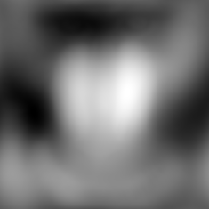
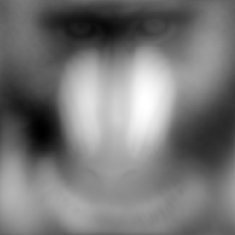
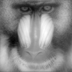
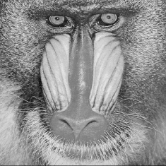
Figure 1: Fractional integration applied to the Mandrill image wolfram appears to blur the image somewhat analogous to the blurring of integer-valued integrations. This shows $q=-1.8$ (upper-left), $q=-1.3$ (upper right), $q=-0.6$ (lower left), and $q=0$ (the original image on the lower right).

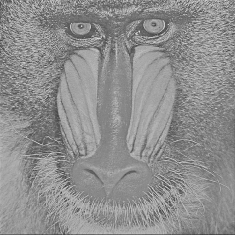
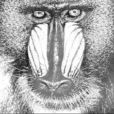
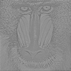
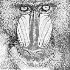
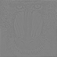
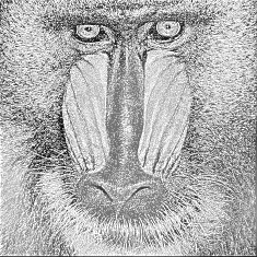
Figure 2: Fractional differentiation applied to the Mandrill image wolfram operates analogously to integer-valued derivatives. The left column shows the fractional derivatives while the right column shows an edge-detection-like thresholding of the fractional derivative added to the image (a common way to visualize derivative-like actions on images gonzales ). Shown are $q=1$ (the normal derivative, bottom), $q=0.55$ (middle), and $q=0.25$ (top). Different $q$ values show different levels of detail.

Section II presents the key idea of the Riesz differintegrals as a variation on standard Fourier methods. Section III shows how the frequency domain definitions can be used to form the basis of data processing algorithms, and Section IV interprets the intuition behind the method. Section V discusses some interesting and useful properties of the differintegrals, Section VI describes a series of simple applications, and Section VII concludes. Computer code to carry out the required computations are available in both Mathematica and Matlab at the author’s website differintegralSite .

II Defining Differintegrals via the Fourier Transform

The Fourier transform of an absolutely integrable function $f(t)$ on the interval $(-\infty,\infty)$ is a complex-valued function $F(\omega)$ of frequency $\omega$ defined by

$$F(\omega)=\mathcal{F}\{f(t)\}=\int_{-\infty}^{\infty}f(t)e^{-j\omega t}dt.$$ (1)

The inverse Fourier transform can be similarly written as $\mathcal{F}^{-1}\{F(\omega)\}=f(t)$. A fundamental result relates the time-derivative of the function to the transform

$$\mathcal{F}\{\frac{df(t)}{dt}\}=j\omega F(\omega).$$ (2)

Assuming that all the derivatives, $f^{\prime}(t),\ldots,f^{(n-1)}(t),$ vanish as $t\rightarrow\pm\infty,$ this can be iterated $n$ times to express the $n$th derivative in terms of the Fourier transform

$$\mathcal{F}\{\frac{d^{n}f(t)}{dt^{n}}\}=(j\omega)^{n}F(\omega).$$ (3)

Similarly, it is possible to express the time-integral of a function in terms of its Fourier transform. Let $g(t)=\frac{df(t)}{dt}$, substitute into (2), and rearrange to find

$$\mathcal{F}\{\int_{-\infty}^{t}g(\tau)d\tau\}=\frac{1}{j\omega}\mathcal{F}\{g(t)\}=\frac{1}{j\omega}G(\omega).$$ (4)

Observe that (4) is correct only up to a constant since taking the derivative of $f$ removes any “DC” value.

The key idea of the Riesz fractional definition is to rewrite (3) as

$$\mathbf{D}^{q}(f)=\frac{d^{q}f(t)}{dt^{q}}=\mathcal{F}^{-1}\{|\omega|^{q}F(\omega)\}$$ (5)

and to consider this to be a definition: the $q$th derivative of the function $f(t)$ with respect to $t$ is defined to be the inverse Fourier transform of $|\omega|^{q}$ times the Fourier transform of $f(t)$. The usefulness of this approach is that $q$ need not be an integer. Moreover, $q$ need not be positive. When $q=-1$, for instance, this recaptures the relationship in (4); when $q=1$, (5) recaptures (3) (but for the absolute value signs). Hence (5) suffices to define both fractional derivatives (when $q$ is positive) and fractional integrals (when $q$ is negative).

Some care is needed to make the above argument precise. First, the formal definition (details can be found in Appendix A) divides the Fourier transform into two parts (one from $-\infty$ to $t$ and the other from $t$ to $\infty$) and it is necessary to replace $(j\omega)$ by $|\omega|$ to ensure that both integrals converge. Second, the raising of a number to a fractional power does not have a unique answer, but can result in multiple possible answers (for example, $n^{1/2}$ can assume two possible values, one positive and one negative). This can cause sign ambiguities in the value of the fractional derivatives or integrals. Third, it may be advantageous in some situations to weight the two halves of the Fourier transform, as suggested by Feller. In this generalization, (5) is replaced by

$$\mathbf{D}^{q}f=\mathcal{F}^{-1}\{\left[c_{1}(\theta,q)(j\omega)^{q}+c_{2}(\theta,q)(-j\omega)^{q}\right]F(\omega)\}.$$ (6)

For details, see Appendix A.4.

III Computing Differintegrals

The defining equation (5) is not only a theoretical definition, it can also be used as a basis for computation by replacing the Fourier transform with the Discrete Fourier Transform (DFT). Given a data sequence $f$ of length $n$, let $w$ be a length-$n$ frequency vector spanning normalized frequency $[-1,1]$. The $q$th fractional differintegral is straightforwardly implemented in pseudocode as

$$\mbox{IFFT( Abs(w)}^{\wedge}\mbox{q}\mbox{ FFT(f) )}$$ (7)

where the power is an element-by-element operation and where FFT and IFFT represent the DFT and its inverse. This is shown in block diagram form in Figure 3.

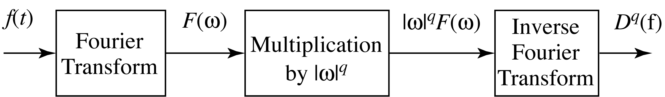
Figure 3: The fractional derivative (or integral) of a function $f(t)$ can be calculated straightforwardly in the frequency domain using (7).

Perhaps the simplest case is $q=1$, using (7) to calculate the (regular) derivative. Normally, this would be a waste of computational effort since there are efficient algorithms for calculating derivatives (finite differences, differential quadrature, etc.) and (7) requires two DFTs. But it is worth considering an example that shows how (7) assumes periodicity. Figure 4 shows two examples of derivatives calculated via this method; in the top, the function is periodic and the derivative appears plausible. For example, it is positive when the slope of the sampled function is increasing and goes to zero when the sampled function flattens out. In the bottom example, the derivative is not (as might be expected) closely related to the derivative of the implied sampled function (a parabola), but rather is the derivative of one period of the periodic extension. This same factor occurs in all differintegrals calculated via the method (5)-(7). It can be ameliorated by windowing (which tapers both ends of the function to zero).

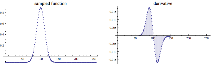
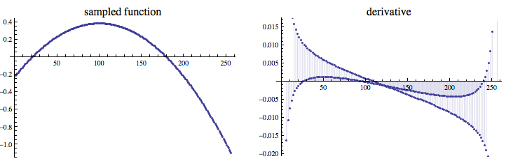
Figure 4: Calculating a derivative using the DFT method (5)-(7) may give unexpected results (bottom curves) when the function is not periodic.

Figure 5 shows various fractional integrals and fractional derivatives of the sampled function from the top row of Figure 4. These also incorporate the Feller “skew” parameters $c_{1}(\theta,q)$ and $c_{2}(\theta,q)$ which weight the contributions from the two halves of the Fourier transform, replacing (5) with (6) and (7) with

$$\mbox{IFFT( c1*(j w)}^{\wedge}\mbox{q}\mbox{+ c2*(-j w)}^{\wedge}\mbox{q}\mbox{ FFT(f) )}$$ (8)

where c1 and c2 are given by (29)-(30) as in Appendix A.4.

In one dimension, w (of (7)) is a vector that represents normalized frequency. In two dimensions, w is a matrix that represents two dimensions $(\omega_{1},\omega_{2})$ of normalized frequency, the Abs function is the norm $\mbox{Abs}(\sqrt{\omega_{1}^{2}+\omega_{2}^{2}})$, and FFT and IFFT represent the two-dimensional Discrete Fourier transform and its inverse. Examples in two dimensions are shown in Figures 1 and 2, demonstrating that the methods apply equally well to images as to one dimensional signals.

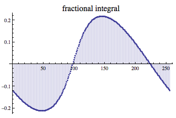
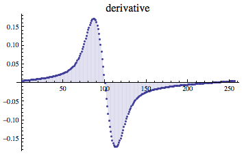
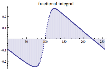
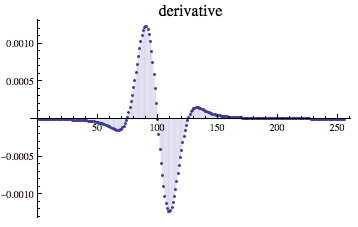
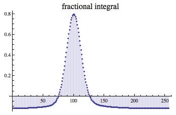
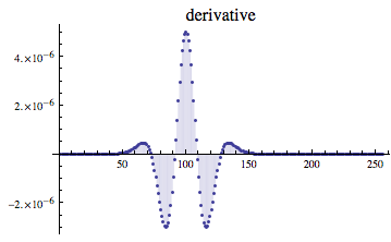
Figure 5: Using the sampled function from the top-left of Figure 4, several differintegrals are calculated using the DFT method (5)-(7). The left column (from top to bottom) has integrals with $q=-2.3,-1.05,-0.1$ and skew parameters $\theta=1,1,0$, while the right column has $q=0.3,1.8,3.6$ and skew parameters $\theta=1,1,0$.

Integer-valued derivatives are local, in the sense that the derivative of a function at a point depends only on the values of the function near that point. In contrast, differintegrals are nonlocal; the value of the differintegral at a point depends on all values of the function. This means that there is no simple time-domain formula (like the discrete difference operator or the Euler integration formula) that can calculate numerical differintegrals. Rather, calculation in the time domain requires convolution with an operator that has the same length as the signal. To calculate the derivative at every point is thus an $O(n^{2})$ operation. In contrast, the two FFTs that dominate the calculation of (7) are $O(n\log(n))$. Thus the calculation in the Fourier domain is more straightforward to carry out when compared to the time-domain convolution, and it is also computationally advantageous.

IV Interpreting Differintegrals

The defining equation (5) can also be used to gain insight into the meaning of the fractional-order filters defined by applying the differintegral operations to a signal. The right hand side contains a product of two frequency domain terms

$$F(\omega)=\mathcal{F}\{f(t)\}\mbox{ and }|\omega|^{q}.$$

The first is the Fourier transform (1) of the signal that is being operated on. The second is frequency, raised to a fractional power. Figure 6 plots this function for a range of $q$. The plot is divided into two parts, $q>0$ on the left and $q<0$ on the right. The frequency axis is normalized to $(-1,1)$.

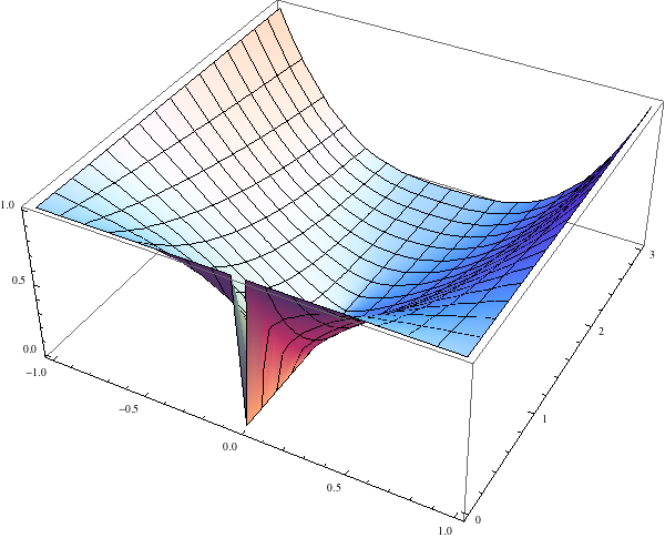
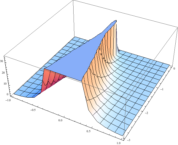
Figure 6: Plot of $H(\omega)=|\omega|^{q}$ is divided into two parts. On the left is $3>q>0$, which shows the frequency scaling accomplished by the fractional derivatives. On the right, $-3<q<0$, showing the frequency scaling accomplished by the fractional integrals. These can be interpreted as the frequency response of the “system” defined by the Riesz differintegral (5).

The convolution property of Fourier transforms relates the convolution (denoted $\ast$) of two functions to the product of their transforms. Thus

$$\mathcal{F}\{g(t)\ast h(t)\}=\mathcal{F}\{g(t)\}\mathcal{F}\{h(t)\}=G(\omega)H(\omega).$$ (9)

In the filtering application, $g(t)$ may be interpreted as a signal and $h(t)$ may be interpreted as the impulse response of a system. The output of the system can be calculated either by convolving in the time domain or by multiplying in the frequency domain. The frequency content of the output is interpreted as the product of the transform of the input and the frequency response of the system. In the differintegral setting, $g(t)$ may be interpreted as the signal to be processed and $h(t)$ is the impulse response of the system. Since $H(\omega)=|\omega|^{q}$, the impulse response is $h(t)=\mathcal{F}^{-1}\{H(\omega)\}=\mathcal{F}^{-1}\{|\omega|^{q}\}$.

For example, consider the fractional order derivative of a function $f(t)$ which has Fourier transform $F(\omega)$. According to (5), the transform of this derivative is the product of $F(\omega)$ and $H(\omega)=|\omega|^{q}$. A typical contour of such a function is shown in the left hand side of Figure 6. It is $1$ at high frequencies and descends smoothly (at least as long as $q>0$) to zero at $\omega=0$. In words, this is a kind of highpass filter which passes high frequencies and attenuates low frequencies. Thus the fractional derivative can be interpreted as highpass operation.

Analogously, consider the fractional order integral of a function $f(t)$ which has Fourier transform $F(\omega)$. According to (5), the transform of this integral is the product of $F(\omega)$ and $H(\omega)=|\omega|^{q}$, where now $q<0$. A typical contour of such a function is shown in the right hand side of Figure 6. It is $1$ at high frequencies and ascends continuously towards infinity as $\omega$ approaches zero. In words, this is a kind of lowpass filter which emphasizes low frequencies in comparison to high frequencies. Thus the fractional integral can be interpreted as lowpass operation.

By the convolution property (9), these differintegrals can be calculated in the frequency domain (as in Section III) or by calculating $h(t)$ and then convolving in the time domain. Indeed, a significant amount of effort is required to write $h(t)$ explicitly, and the formulas in herrmann and mathieu are complicated, involving $\Gamma$ functions and collections of factorials. Moreover, the branch cut problems in these inversions can be formidable, limiting the validity of the formulas to small ranges of values of $q$.

V Properties of Differintegrals

Fractional-order derivatives and integrals are closely related to integer-order derivatives and integrals, in the sense that they share a common origin (in the Riesz definition (5) at least) and a common interpretation as lowpass and/or highpass filters as given by the frequency response $H(\omega)$ of Figure 6. It should come as no surprise that they also share many properties, and this section details some of these properties.

1. Linearity: Differintegrals are linear in the sense that

   $$\mathbf{D}^{q}(a_{1}f_{1}+a_{2}f_{2})=a_{1}\mathbf{D}^{q}f_{1}+a_{2}\mathbf{D}^{q}f_{2},$$ (10)

   where $a_{1}$ and $a_{2}$ are constants and $f_{1}(t)$ and $f_{2}(t)$ are Fourier integrable functions. This follows immediately from the linearity of the integrals.

2. Composition: The differintegrals $\mathbf{D}^{q_{1}}$ and $\mathbf{D}^{q_{2}}$ can be composed so that

   $$\mathbf{D}^{q_{1}}\left(\mathbf{D}^{q_{2}}f\right)=\mathbf{D}^{q_{2}}\left(\mathbf{D}^{q_{1}}f\right)=\mathbf{D}^{q_{1}+q_{2}}f.$$ (11)

   The composition rule can be demonstrated by applying the definition (5) to $\mathbf{D}^{q_{2}}f$, then to $\mathbf{D}^{q_{1}}f$, and then simplifying

   $$\mathbf{D}^{q_{1}}\left(\mathbf{D}^{q_{2}}f\right) =\mathbf{D}^{q_{1}}\left(\mathcal{F}^{-1}\left\{\left|\omega\right|^{q_{2}}F(\omega)\right\}\right)$$

   $$=\mathcal{F}^{-1}\left\{\left|\omega\right|^{q_{1}}\mathcal{F}\left\{\mathcal{F}^{-1}\{\left|\omega\right|^{q_{2}}F(\omega)\}\right\}\right\}$$

   $$=\mathcal{F}^{-1}\left\{\left|\omega\right|^{q_{1}}\left|\omega\right|^{q_{2}}F(\omega)\right\}$$

   $$=\mathcal{F}^{-1}\left\{\left|\omega\right|^{q_{1}+q_{2}}F(\omega)\right\}=\mathbf{D}^{q_{1}+q_{2}}f.$$

   In general, RL differintegrals only commute under special circumstances bayin (having to do with the boundary conditions of the RL Laplace transform, as discussed in Appendix A.2). In the present case the required boundary conditions are fulfilled because of the assumption of the existence of the Fourier transform of the function $f$.

3. Identity: A special case of (11) is when $q_{1}=-q_{2}$

   $$\mathbf{D}^{q}\left(\mathbf{D}^{-q}f\right)=\mathbf{D}^{-q}\left(\mathbf{D}^{q}f\right)=\mathbf{D}^{0}f=f.$$

   For a given $f$, the differintegrals form a commutative group with identity $\mathbf{D}^{0}$ and where the inverse of element $\mathbf{D}^{q}$ is $\mathbf{D}^{-q}$. This can be interpreted from a “block diagram” perspective as saying that differintegral operators act like linear elements where differintegral blocks may be combined and rearranged in many of the same ways that linear time-invariant transfer functions can be combined and rearranged.

4. Leibniz’s Rule: The differintegral of the $q$th order of the multiplication of two functions $f$ and $g$ is given by the formula

   $$\mathbf{D}^{q}(fg)=\sum_{k=0}^{\infty}\binom{q}{k}\mathbf{D}^{q-k}(f)\ \mathbf{D}^{k}(g),$$ (12)

   where the binomial coefficients are calculated by replacing the factorials with the corresponding gamma functions.

In terms of Fourier analysis, differintegrals are a special case of multiplier operators duoandikoetxea , translation-invariant operators that reshape the frequencies in a function. Many of the computational results of Section III hold for general multiplier operators and much of the frequency-domain intuition of Section IV still apply in this more general setting, though the details will change to reflect the specifics of the multiplier under consideration.

VI Applications

This paper began with a series of motivating images processed by the differintegral operator: Figure (1) showed the smoothing operations performed by fractional integrations and Figure (2) showed some simple edge detectors based on fractional derivatives. This section presents a small number of other applications that might benefit from the use of differintegral filters and illustrates the use of some of the parameters.

VI.1 Application of Skew Parameter to Embossing

This example fixes the fractional derivative at $q=0.5$ and examines the effect of several different skew parameters (see (6) and (30)) as shown in Figure 7. The appearance is analogous to an embossing effect, which is often accomplished using a collection of directional derivatives. Here the effect is accomplished by changing the skew parameter, which weights the contributions of the positive and negative frequency powers. Changing the skew parameter can make the embossing effect appear to project either inwards or outwards.

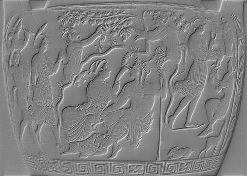
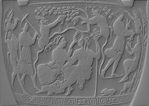
Figure 7: The original image of the vase is in the upper left. The fractional derivative with $q=0.5$ is shown with three different skew values, $\theta=0$ (negative, upper right), $\theta=0.3$ (positive, lower left) and $\theta=0.6$ (negative, lower right). The results are like variations on an embossing effect.

VI.2 Application to Eclipse Detection

An exoplanet transiting a distant star appears as a periodic dip in the brightness of the star kepler . Assuming that the radius $R_{s}$ of the star is much larger than the radius $R_{p}$ of the planet, the change in the brightness is approximately proportional to the area

$$A(t) =\frac{R^{2}}{2}(\theta(t)-\sin\theta(t))$$ (13)

$$\theta(t) =2\arccos(1-vt/R),\text{ }t\in(0,2r/v)$$

where $R$ is radius of the image of the planet cast on the star, $t$ is the time, $v$ is the velocity of the planet, and $\theta$ is the angle shown in Figure 8.

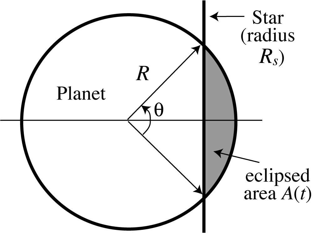
Figure 8: The shaded area $A(t)$ of (13) is the region eclipsed by the planet as it traverses the star.

For simplicity, assume that the transit occurs on the equatorial plane of the star. The radius of the image of the planet on the star is $R=R_{p}\frac{d_{s}}{d_{p}}$, where $d_{s}$ and $d_{p}$ are the distances of the star and the planet from the point of observation. After the planet moves completely within the field of the star, the brightness remains constant at its minimum level until the planet begins its exit on the other side. The brightness of a star can be written

$$b=\frac{\pi R_{s}^{2}I_{s}}{d_{s}^{2}},$$

where $I_{s}$ is the intensity. The fractional change in brightness is

$$\frac{\Delta b}{b} =\frac{\left(\pi R_{s}^{2}-A(t)\right)I_{s}/d_{s}^{2}}{b}$$

$$=1-\frac{A(t)}{\pi R_{s}^{2}}.$$ (14)

This is plotted in the top left portion of Figure 9 and a modest amount of noise is added in the top right. The first derivative (middle left) shows the location of the points of inflection because these are the points where the rate of change is largest. In the noisy version, however, the locations of the inflection points are overwhelmed by the noisiness of the derivative. The $q=0.5$ derivative (with a skewness of $1$) is shown in the bottom two parts. Without noise (bottom left), the location of the inflection points is clear; with noise (bottom right), the inflection points are still clear, though the precise locations may be difficult to pinpoint. In this case, the $q=0.5$ derivative would be preferred to the $q=1$ derivative for the purpose of locating the points of maximum change. This can be viewed as an application of the CRONE detector mathieu to the brightness function (14).

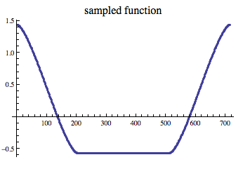
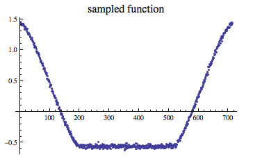
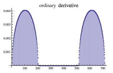
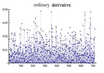
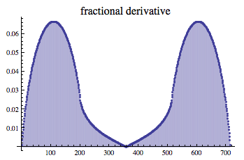
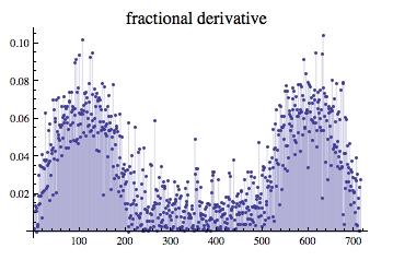
Figure 9: The fractional change in brightness (14) is plotted in the top left for some nominal values of the parameters. A modest amount of noise (compare to Figure 2 of kepler ) is added in the top right. The absolute value of the $q=1$ derivative of the brightness is shown in the middle left; this has two peaks which show the inflection points of the brightness curve. The absolute value of the $q=1$ derivative of the noisy brightness is shown in the middle right; the noise destroys information about the location of the inflection points. The absolute value of the $q=0.5$ derivative of the brightness is shown in the bottom left; this again has two peaks which show the inflection points. The absolute value of the $q=0.5$ derivative of the noisy brightness is shown in the bottom right. Even in the presence of the noise, the approximate location of the inflection points can still be determined.

VI.3 Processing Colored Images

One approach to the processing of colored images is to filter the red, green, and blue (RGB) channels separately. While this can sometimes be effective, the colors in the output may be different from the colors in the original. When this is undesirable, a common approach is to translate the RGB channels into the hue-saturation-brightness (HSB) colorspace, to process the brightness channel alone, and then convert back to RGB for display. This tends to preserve the hue and saturation (the “color”) while changing the brightness. As with (integer-valued) derivative and integral operators, this can be an effective means of applying differintegral operations to color images.

A series of such images (with different values of $q$ and different skew values) are shown at the website differintegralSite . These include a collection of differently smoothed $q<0$ and sharpened $q>0$ versions of the mandrill image from Figures 1 and 2. Visual effects include smooth blurs, edge-like extractions, and posterizations (when used in conjunction with binarization) depending on the particular parameters chosen. Also on the website are several interactive demonstrations, written in the Wolfram .cdf format (see differintegralSite for links). These can be used inside of Mathematica, or can be used by downloading the free .cdf player from the Wolfram website. The demonstrations allow the user to “play with” the differintegral operators in a straightforward way.

VII Conclusions

Fractional order derivatives and integrals are sensible tools that should be in the practitioner’s signal processing toolbox. While it is unreasonable to expect miraculous new kinds of processing effects from these tools, they do provide a logical extension to current techniques. Since derivatives and integrals are at the heart of many different classical signal processing algorithms, it is reasonable to ask, in each case, whether the use of fractional-order filters may enhance these applications. In order to test whether the methods are useful in a given application, the authors provide computer code in both Mathematica and in Matlab to easily carry out the required calculations differintegralSite .

Appendix A Basic Definitions

Appendix A.1 begins with the Riemann-Liouville (RL) definitions of fractional integrals and derivatives. Transforming into the frequency domain, as in Appendices A.2 and A.3, allows restatement of the definitions that hold under fairly general conditions. This formulation was first described by Riesz riesz . Finally, Appendix A.4 provides a useful extension to the case where the two parts of the differintegrals are weighted appropriately.

A.1 RL Definition of Differintegrals

The $q$th (right hand) fractional integral of a function is defined to be

$$_{a^{+}}\mathbf{D}_{t}^{-q}f(t)=\frac{1}{\Gamma(q)}\int_{a}^{t}(t-\tau)^{q-1}f(\tau)d\tau$$ (15)

where $\Gamma(q)$ is the gamma function, $a<t$, and $q>0$. At first it might seem odd to use the letter $\mathbf{D}^{-q}$ for an integral; doing so allows a unified notation where a positive exponent means “derivative” and a negative exponent means “integral.” When $q=1$, this corresponds to the “regular” integral from $a$ to $t$ of the function $f(\tau)$. The definition of the fractional derivative is less straightforward because the integral in (15) diverges for $q\leq 0$. This can be addressed as in bayin by taking the $n$th (integer) derivative composed with the $0<n-q<1$ fractional integral where $n=\lceil q\rceil$ is the smallest integer larger than $q$. Accordingly, the $q$th (right hand) fractional derivative is defined as

$$_{a^{+}}\mathbf{D}_{t}^{q}f(t)=\frac{d^{n}}{dt^{n}}\left({}_{a^{+}}\mathbf{D}_{t}^{q-n}f(t)\right).$$ (16)

Similarly, The RL (left handed) integral and derivative are

$$_{b^{-}}\mathbf{D}_{t}^{-q}f(t)=\frac{1}{\Gamma(q)}\int_{t}^{b}(\tau-t)^{q-1}f(\tau)d\tau$$ (17)

$$_{b^{-}}\mathbf{D}_{t}^{q}f(t)=(-1)^{n}\frac{d^{n}}{dt^{n}}\left({}_{b^{-}}\mathbf{D}_{t}^{q-n}f(t)\right),$$ (18)

where $t<b$, $n=\lceil q\rceil$, and $q>0$. The most common values $a=-\infty$ and $b=\infty$ are also called the Weyl differintegral.

A.2 Riesz Fractional Integral

The Riesz formula arises from the Fourier transform of the right-hand fractional RL integral (15) with $a=-\infty$

$$_{-\infty}\mathbf{D}_{t}^{-q}g(t)=\frac{1}{\Gamma(q)}\int_{-\infty}^{t}(t-\tau)^{q-1}g(\tau)d\tau,\text{ }q>0.$$ (19)

To calculate this integral, write the Laplace transform of the function $h(t)=\frac{t^{q-1}}{\Gamma(q)}$ for $q>0$ as

$$\pounds\{h(t)\}=\frac{1}{\Gamma(q)}\int_{0}^{\infty}t^{q-1}e^{-st}dt=s^{-q}.$$

Next, substitute $s=j\omega$ to obtain the Fourier transform of

$$h_{+}(t)=\left\{\begin{tabular}[]{ll}$\dfrac{t^{q-1}}{\Gamma(q)},$&$t>0,$\\ $0$&$t\leq 0$\end{tabular}\ \right.$$

which is

$$\mathcal{F}\{h_{+}(t)\}=(j\omega)^{-q},\text{ }q>0.$$

The convolution of $h_{+}(t)$ and $g(t)$ is

$$h_{+}(t)\ast g(t) =\int_{-\infty}^{\infty}h_{+}(t-\tau)g(\tau)d\tau$$

$$=\frac{1}{\Gamma(q)}\int_{-\infty}^{t}(t-\tau)^{q-1}g(\tau)d\tau$$

$$=_{-\infty}\mathbf{D}_{t}^{-q}g(t)$$

as in (19). Using the convolution property of the Fourier transform (9), this becomes

$$\mathcal{F}\{_{-\infty}\mathbf{D}_{t}^{-q}g(t)\}=(j\omega)^{-q}G(\omega),\mbox{ for }q>0$$ (20)

where $G(\omega)$ is the Fourier transform of $g(t)$. Similarly, the left-hand RL integral (17) with $b=\infty$ is

$${}_{\infty}\mathbf{D}_{t}^{-q}g(t)=\frac{1}{\Gamma(q)}\int_{t}^{\infty}(\tau-t)^{q-1}g(\tau)d\tau,\text{ }q>0.$$

After similar manipulations, this becomes

$$\mathcal{F}\{_{-\infty}\mathbf{D}_{t}^{-q}g(t)\}=(-j\omega)^{-q}G(\omega),\text{ }q>0.$$ (21)

Summing (20) and (21) gives gives

$$\mathcal{F}\{\left[{}_{-\infty}\mathbf{D}_{t}^{-q}+_{\infty}\mathbf{D}_{t}^{-q}\right]g(t)\} =\left[(j\omega)^{-q}+(-j\omega)^{-q}\right]G(\omega)$$

$$=\left|\omega\right|^{-q}\left[j^{-q}+(-j)^{-q}\right]G(\omega)$$

$$=\left(2\cos\frac{q\pi}{2}\right)\left|\omega\right|^{-q}G(\omega).$$ (22)

The combined expression elsayed , which is valid for positive $q$ with $q\neq 1,3,5,\ldots$ is

$$\mathbf{D}^{-q}(g) =\frac{1}{2\Gamma(q)\cos\left(\frac{q\pi}{2}\right)}\int_{-\infty}^{\infty}(t-\tau)^{q-1}g(\tau)d\tau$$

$$=\frac{\left[{}_{-\infty}\mathbf{D}_{t}^{-q}+_{\infty}\mathbf{D}_{t}^{-q}\right]g(t)}{2\cos\left(\frac{q\pi}{2}\right)}$$

$$=\mathcal{F}^{-1}\{\left|\omega\right|^{-q}G(\omega)\}.$$ (23)

This is the Riesz fractional integral. The final equality results from taking the inverse Fourier transform of both sides of (A.2), after dividing by the term $2\cos\left(\frac{q\pi}{2}\right)$.

A.3 Riesz Fractional Derivative

Substituting (15) into the RL derivative (16) with $a=-\infty$ and $q$ positive gives

$$_{-\infty}\mathbf{D}_{t}^{q}g(t) =\frac{1}{\Gamma(n-q)}\int_{-\infty}^{t}(t-\tau)^{-q-1+n}g^{(n)}(\tau)d\tau$$

$$=_{-\infty}\mathbf{D}_{t}^{q-n}g^{(n)}(t),\mbox{ for }n-1<q<n,$$ (24)

where $g(t)$ and its derivatives are assumed integrable. Since $q-n<0,$ (20) can be used to write the Fourier transform of (A.3) as

$$\mathcal{F}\{_{-\infty}\mathbf{D}_{t}^{q}g(t)\} =(j\omega)^{q-n}\mathcal{F}\{g^{(n)}(t)\},\text{ }q>0,$$

$$=(j\omega)^{q-n}(j\omega)^{n}G(\omega)$$

$$=(j\omega)^{q}G(\omega).$$ (25)

Similarly,

$$\mathcal{F}\{_{\infty}\mathbf{D}_{t}^{q}g(t)\}=(-j\omega)^{q}G(\omega).$$ (26)

Combining the results in (A.3) and (26) gives

$$\mathcal{F}\{\left[{}_{-\infty}\mathbf{D}_{t}^{q}+_{\infty}\mathbf{D}_{t}^{q}\right]g(t)\} =\left[(j\omega)^{q}+(-j\omega)^{q}\right]G(\omega)$$

$$=\left(2\cos\frac{q\pi}{2}\right)\left|\omega\right|^{q}G(\omega).$$ (27)

For $0<q\leq 2$, $q\neq 1,$ the Riesz fractional derivative is defined herrmann as

$$\mathbf{D}^{q}(g)=-\frac{\left[{}_{-\infty}\mathbf{D}_{t}^{q}+_{\infty}\mathbf{D}_{t}^{q}\right]g(t)}{2\cos\left(\frac{q\pi}{2}\right)}.$$ (28)

The minus sign in (28) is introduced to recover the $q=2$ case

$$\mathbf{D}^{2}(g) =-\frac{1}{2\pi}\int_{-\infty}^{\infty}\left|\omega\right|^{2}G(\omega)e^{j\omega t}d\omega$$

$$=\frac{1}{2\pi}\int_{-\infty}^{\infty}G(\omega)\left[\frac{d^{2}}{dt^{2}}e^{j\omega t}\right]d\omega$$

$$=\frac{d^{2}}{dt^{2}}\left[\frac{1}{2\pi}\int_{-\infty}^{\infty}G(\omega)e^{j\omega t}d\omega\right]$$

$$=\frac{d^{2}}{dt^{2}}g(t).$$

A.4 The Feller Derivative

The linear combination

$$\mathbf{D}_{\theta}^{q}f(t)=\left[c_{1}(\theta,q)_{-\infty}\mathbf{D}_{t}^{q}+c_{2}(\theta,q)_{\infty}\mathbf{D}_{t}^{q}\right]f(t)$$ (29)

where

$$c_{1}(\theta,q) = -\frac{\sin((q+\theta)\pi/2)}{\sin\pi\theta}$$

$$c_{2}(\theta,q) = -\frac{\sin((q-\theta)\pi/2)}{\sin\pi\theta}$$ (30)

has been introduced by Feller as a generalization of fractional derivatives. This weights the left and right-hand differintegrals according the $c$ parameters and allows extra flexibility in the calculations. The parameter $\theta$ is called the phase or the skew factor. Two special cases are of note:

1. For $\theta=0$, $c_{1}(0,q)=c_{2}(0,q)=-\frac{1}{2\cos(q\pi/2)}$, and the Feller derivative $\mathbf{D}_{\theta=0}^{q}(f)$ reduces to the Riesz derivative $\mathbf{D}^{q}(f)$.

2. For $\theta=1$, $c_{1}(1,q)=-c_{2}(1,q)=-\frac{1}{2\sin(q\pi/2)}$, and the Feller derivative combines the left and right-handed derivatives with opposite signs

   $$\mathbf{D}_{\theta=1}^{q}(f)=\frac{\left[{}_{-\infty}\mathbf{D}_{t}^{q}-_{\infty}\mathbf{D}_{t}^{q}\right]}{2\sin(q\pi/2)}f(t).$$

   Up to a constant, this case is the same as the “CRONE detector” derived in mathieu in the time domain.

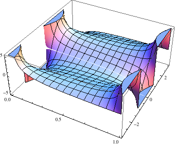
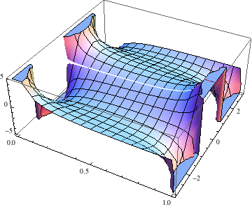
Figure 10: Plot of the weighting coefficients $c_{1}(\theta,q)$ and $c_{2}(\theta,q)$ for $-3<q<3$ and $0<\theta<1$.

References

- (1) R. Hilfer (ed.), Fractional Calculus: Applications in Physics, World Scientific ( 2000).
- (2) K. B. Oldham and J. Spanier, The Fractional Calculus, Dover (1974).
- (3) S. Das, Functional fractional calculus for system identification and controls, Springer, 2007.
- (4) R. Herrmann, http://arxiv.org/abs/0906.2185v2
- (5) A. A. Kilbas, H. M. Srivastava and J. J. Trujillo, Theory and Applications of Fractional Differential Equations, Elsevier (2006).
- (6) I. Podlubny, Fractional Differential Equations, Academic Press ( 1999).
- (7) Igor M. Sokolov, Joseph Klafter and Alexander Blumen, Physics Today, November (2002).
- (8) N. Laskin, Fractional quantum mechanics, Phys. Rev. E62 (2000) 3135.
- (9) S. S. Bayin, Time fractional Schrödinger equation:Fox’s H-functions and the effective potential, J. Math. Phys., 54, 012103, 2013.
- (10) S. S. Bayin, Consistency problem of the solutions of the space fractional Schrödinger equation, 54, 092101, 2013.
- (11) T. T. Hartley and C. F. Lorenzo, Fractional system identification: an approach using continuous order distributions, Technical report, National Aeronautics and Space Administration Glenn Research Center NASA TM, 1999..
- (12) G. Maione and P. Lino, New tuning rules for fractional controllers, Nonlinear Dynamics, 49, Springer, 2007.
- (13) B. T. Krishna and K. V. V. S. Reddy, Design of digital differentiators and integrators of order 1/2, World Journal of Modelling and Simulation, UK, 4:182-187, World Academic Press, 2008.
- (14) B. Mathieu, P. Melchior, A. Oustaloup, Ch. Ceyral, Fractional differentiation for edge detection, Signal Processing 83, pp. 2421Ğ2432, 2003.
- (15) M. D. Ortigueira, J. A. T. Machado, and J. S. da Costa, Which differintegration? [fractional calculus], Vision, Image and Signal Processing, IEE Proceedings, 152, no.6, pp. 846- 850, 9 Dec. 2005.
- (16) C. C. Tseng and S. L. Lee, Digital image sharpening using fractional derivative and Mach band effect, IEEE, International Symposium on Circuits and Systems, pp.1122-1127, Dec 2012.
- (17) S. Khanna and V. Chandrasekaran, Fractional derivative filter for image contrast enhancement with order prediction, IET International Conference on Image Processing, London, UK; 07/2012.
- (18) Y. Ye, X. Pan, J. Wang, Identification of blur parameters of motion blurred image using fractional order derivative, The 11th International Conference on Information Sciences, Signal Processing and their Applications:Main Tracks, 539, 2012.
- (19) J. Bai and X. C. Feng, Fractional-order anisotropic diffusion for image denoising, IEEE Transactions on Image Processing, 16, 2492-2502, 2007.
- (20) E. Cuesta, M. Kirane and S. A. Malik, Image structure denoising using generalized fractional time integrals, Signal Processing, 92, 553-563, 2012.
- (21) M. Janev, S. Pilipovic, T. Atanackovic and R. Obradovic, Fully fractional anisotropic diffusion for image denoising, Mathematical and Computer Modelling, 54, 729-741, 2011.
- (22) Z. Jun and W. Zhihui, A class of fractional-order mult-scale variational models and alternating projection algorithm for image denoising, Applied Mathematical Modelling, 35, 2516-2528, 2011.
- (23) Y. F. Pu, J.L. Zhou and X. Yuan, Fractional differential mask: A fractional differential-based approach for multiscale texture enhancement, EEE Transactions on Image Processing, 19, 491-511, 2010.
- (24) H. Yang, Y. Y. D. Wang and B. Jiang, A novel fractional-order signal processing based on edge detection method, 11th Int. Conf. Control, Automation, Robotics and Vision, Singapure, pp. 1122-1127, 7-10th Dec., 2010.
- (25) A. Nakib, H. Oulhadj, P. Siarry, A thresholding method based on two-dimensional fractional differentiation, Image and Vision Computing, 27, 1343-1357, 2009.
- (26) A. Nakib, H. Oulhadj and P. Siarry, Fractional differentiation and non-pareto multiobjective optimization for image threshholding, Engineering Applications of Artificial Intelligence, 22, 236-249, 2009.
- (27) P. Ghamisi, M. S. Couceiro, J. A. Benediktsson and N. M. F. Ferreira, An efficient method for segmentation of images based on fractional calculus and natural selection, Expert Systems with Applications, 39, 12407-12417, 2012.
- (28) R. J. Barton and H. V. Poor, Signal detection in Fractional Gaussian Noise, IEEE Transactions on Information Theory, 34, 943-959, 1988.
- (29) A. Prasad, M.Kumar, D. R. Choudhury, Color image encoding using fractional transformation associated with wavelet transformation, Optics Communications, 285, 1005-1009, 2012.
-
(30)
Website containing Mathematica and
Matlab code for calculating one and two dimensional differintegrals.
- (31) Wolfram curated image data “Mandrill,” http://reference.wolfram.com/ mathematica/ref/ExampleData.html
- (32) R. C. Gonzales and R. E. Woods, Digital image processing, 3rd Ed, Prentice Hall, 2008.
- (33) S. S. Bayin, Mathematical Models in Science and Engineering, Wiley, 2006.
- (34) J. Duoandikoetxea, Fourier analysis, American Mathematical Society, 2000.
- (35) “Kepler and the transit of Venus,” http://kepler.nasa.gov/files/mws/ Candidates_poster_back_28Dec11_print.pdf
- (36) M. Riesz, Acta Math. 81, 1949.
- (37) A. M. A. El-Sayed and M. Gaber, On the finite Caputo and finite Riesz derivatives, Electrical J. of Theoretical Physics, 3, No. 81, 2006.