Cyclones and attractive streaming generated by acoustical vortices

Abstract

Acoustical and optical vortices have attracted large interest due to their ability in capturing and manipulating particles with the use of the radiation pressure. Here we show that acoustical vortices can also induce axial vortical flow reminiscent of cyclones whose topology can be controlled by adjusting the properties of the acoustical beam. In confined geometry, the phase singularity enables generating ”attractive streaming” with a flow directed toward the sound source. This opens perspectives for contact-less vortical flow control.

I Introduction

Acoustic streaming, that is to say vortical flow generated by sound plays a fundamental role in a variety of industrial and medical applications such as sonochemical reactors Kumar et al. (2007), megasonic cleaning processes Gale and Busnaina (1999), ultrasonic processing Li et al. (2004), acoustophoresis Muller et al. (2012), or therapeutic ultrasound Baker et al. (2001); Crum (2006). More recently, acoustic streaming is the subject of a burst of interest with the development of microfluidic applications Wiklund (2012); Friend and Yeo (2011). For instance, it is at the core of the physics involved in droplets actuation with Surface Acoustic Waves (SAW) Yeo and Friend (2014) for lab-on-a-chip facilities, providing a versatile tool for droplet displacement Wixforth et al. (2004); Renaudin et al. (2006); Brunet et al. (2010), atomization Qi et al. (2008), jetting Shiokawa et al. (1990); Tan et al. (2009) or vibration Brunet et al. (2010); Baudoin et al. (2012); Blamey et al. (2013). Moreover, vorticity associated with acoustic streaming is the main envisioned phenomenon to ensure efficient mixing of liquids Sritharan et al. (2006); Frommelt et al. (2008).

Different forms of streaming are generally distinguished according to the underlying physical mechanism Beyer (1997); Riley (2001). Boundary layer-driven streaming Hamilton (2003) arises when an acoustic wave impinges a fluid/solid interface due to viscous stresses inside the viscous boundary layer. This form of streaming can be decomposed between inner streaming, also called Schlichting streaming Schlichting (1932), occurring inside the viscous boundary layer and counter rotating outer streaming outside it Rayleigh (1884). The former is not exclusive to acoustics since it does not require compressibility of the fluid but only the relative vibration of a fluid and a solid. The latter, first enlightened by Lord Rayleigh, can be either seen as the fluid entrainment outside the boundary layer induced by Schlichting streaming or as a consequence of the tangential velocity continuity requirement for an acoustic wave at a fluid/solid boundary. Finally bulk streaming, or so-called Eckart streaming Eckart (1948) is due to the thermo-viscous dissipation of acoustic waves and the resulting pseudo-momentum transfer to the fluid Piercy and Lamb (1954); Sato and Fujii (2001). Since the early work of Rayleigh Rayleigh (1884), many studies have been dedicated to acoustic streaming and the investigation of the influence of various phenomena on the resulting flow, such as unsteady excitation Rudenko and Soluyan (1971); Rudenko and Sukhorukov (1998); Sou et al. (2011), nonlinear acoustic wave propagation Romanenko (1960); Statnikov (1967) or high hydrodynamic Reynolds number Menguy and Gilbert (1999); I. et al. (2013). However, in all these studies, only plane of focalized acoustical waves Nyborg (1998) are considered.

In this paper, we report on bulk acoustic streaming generated by specific solutions of the Helmholtz equation called acoustical vortices. New acoustic streaming configurations are obtained with cyclone-like flows, whose topology mainly depends on the one of the acoustical vortex. Flow streamlines are not only poloidal as in classic bulk streaming Eckart (1948), but also toroidal due to the orbital momentum transfer. This special feature provides an acoustical control of the axial vorticity, while in all forms of acoustic streaming reported up to now, the topology of the induced hydrodynamical vortices is mainly determined by the boundary conditions. Finally, in confined geometries, the azimuthal vorticity can also be tailored by adjusting the properties of the acoustic beam. In this way, attractor and repeller hydrodynamic vortices, corresponding respectively to flow directed toward or away from the sound source, can be obtained.

II Theoretical analysis

Acoustical vortices (or Bessel beams) are helical waves possessing a pseudo orbital angular momentum and a phase singularity on their axis (for orders $\geq 1$). The pitch of the helix $l$ is called order or topological charge Thomas et al. (2010). These waves are separated variables general solutions of the Helmholtz equation in cylindrical coordinates and are therefore not exclusive to acoustics (see e.g. Allen et al. (1992) for their optical counterparts). Separated variables solutions means that their axial and radial behavior are independant, i.e. the diffraction is canceled for infinite aperture and remains weak in others cases Durnin et al. (1987). This enables their controlled synthesis even in confined geometries. Acoustical vortices can be generated by firing an array of piezo-electric transducers with a circular phase shift Hefner and Marston (1999) or using inverse filtering techniques Thomas and Marchiano (2003); Marchiano and Thomas (2008); Brunet et al. (2009). As little as four transducers are enough to develop a first order vortex Hefner and Marston (1999). Recently, it has been observed that their orbital momentum can be transferred to dissipative media which results in a measurable torque for solids He et al. (1995); Volke-Sepulveda et al. (2008) or azimuthal rotation for fluids Anhauser et al. (2012).

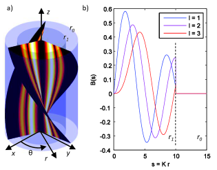
Figure 1: a: Acoustical vortex with topological charge $l=3$, $\tan{(\alpha)=1.21}$ and $Kr_{1}=10$ ($z$-axis was dilated 10 times). Surfaces correspond to the phase $l\theta+k_{z}z=\pi/2$ while colors indicate the magnitude of the radial function $B$. b: Corresponding radial function $B(Kr)$ for $l=1$ to $3$.

In the following, we derive the equations of the flow generated by an attenuated collimated Bessel beam of finite radial extension $r_{1}$ (Fig. 1.a), traveling along the $z$-axis of an unbounded cylindrical tube of radius $r_{0}$. This model constitutes an extension of Eckart’s perturbation theory Eckart (1948) initially limited to plane wave. In the case of Bessel beams Hefner and Marston (1999), the density variation $\rho_{1}$ induced by the acoustical wave takes the form:

$$\rho_{1}(r,\theta,z,t) = \hat{\rho}_{1}B(s)\sin(l\theta+k_{z}z-\omega t),$$ (1)

$$B(s) = A(s)J_{l}(s)$$ (2)

In these equations, $\hat{\rho}_{1}$, $l$, $\theta$, $k_{z}$, $\omega$, $t$ and $J_{l}$ denote respectively the amplitude of the acoustical wave, the topological charge of the Bessel beam, the angular coordinate, the projection of the wave vector on the $z$-axis, the wave angular frequency, the time and the cylindrical Bessel function of order $l$. The spatial window function, $A(s)$, is used to limit the infinite lateral extension of Bessel function. The phase of such vortex is given by $\phi=l\theta+k_{z}z-\omega t$, yielding to helicoidal equiphase surfaces as shown in figure 1.a. We introduce the shorthand notation $s=Kr$, and by analogy $s_{1}=Kr_{1}$, $s_{0}=Kr_{0}$, with $K$ the transversal component of the wave vector. It is defined by the dispersion relation of a Bessel beam: $K^{2}+k_{z}^{2}=\omega^{2}/c^{2}$, with $c$ the sound speed. We also introduce the variable $\alpha$ measuring the helicoidal nature of the flow and defined by $\tan{(\alpha)}=k_{z}/K$. The radial dependence in equation (1) is based on Bessel functions, which are plotted in figure (1.b). Provided that $l\geqslant 1$, these functions cancel at $s=0$, where destructive interference between the wavelets from opposite sides of the vortex occurs. Consequently, the core of the vortex is not solely a phase singularity, but also a shadow-area.

Following Eckart Eckart (1948), acoustic streaming can be calculated by decomposing the flow into a first order compressible and irrotational flow (corresponding to the propagating acoustical wave) and a second order incompressible vortical flow (describing the bulk acoustic streaming). The insertion of this decomposition into Navier-Stokes compressible equations yields Eckart’s diffusion equation for the second order vorticity field $\vec{\varOmega}_{2}=\vec{\nabla}\times\vec{u}_{2}$, with $\vec{u}_{2}$ the second order velocity field. This diffusion is forced by a nonlinear combination of first order terms and simplifies at steady-state into:

$$\Delta\vec{\varOmega_{2}}=-\frac{b}{\rho_{0}^{2}}\vec{\nabla}\rho_{1}\times\vec{\nabla}\frac{\partial\rho_{1}}{\partial t},$$ (3)

with $b=4/3+\mu^{\prime}/\mu$, $\mu^{\prime}$ the bulk viscosity, $\mu$ the shear viscosity, $\rho_{0}$ the density of the fluid at rest and $\rho_{1}$ the first order density variation. Since the streaming flow is incompressible, we can introduce the vector potential $\vec{\Psi}_{2}$ such that $\vec{u}_{2}=\vec{\nabla}\times\vec{\Psi}_{2}$, with Coulomb gauge fixing condition: $\vec{\nabla}.\vec{\Psi}_{2}=0$. The resolution of equation (3) thus amounts to the resolution of the inhomogeneous biharmonic equation: $\Delta^{2}\vec{\Psi}_{2}=-\frac{b}{\rho_{0}^{2}}\vec{\nabla}\rho_{1}\times\vec{\nabla}\frac{\partial\rho_{1}}{\partial t}$. Originally, this equation was integrated by Eckart for truncated plane waves. In the present work, we solve it in the case of Bessel beams, whose expression is given by equations (1) to (2). Owing to the linear nature of this partial differential equation, we consider only solutions verifying the symmetries imposed by the forcing term and the boundary conditions: no-slip condition on the walls, infinite cylinder in the z direction and no net flow along the channel. In this case, the problem reduces to a set of two linear ordinary differential equations, which were integrated with standard methods. The complete procedure is detailed in appendix.

Results are given by equations (II) to (11):

$$u_{2}^{z} = 2\frac{\varOmega^{\star}_{\theta}}{K}\left[\left(1-\frac{s^{2}}{s_{0}^{2}}\right)f(s_{0})\right.$$

$$+ \left.\frac{1}{2}\left(\frac{s^{2}}{{s_{0}}^{2}}\varLambda^{l}_{z}(s_{0})-\varLambda^{l}_{z}(s)\right)\right],$$

$$u_{2}^{\theta} = \frac{\varOmega^{\star}_{z}}{K}\left(\frac{s}{{s_{0}}^{2}}\varLambda^{l}_{\theta}(s_{0})-\frac{1}{s}\varLambda^{l}_{\theta}(s)\right),$$ (5)

with $$f(s)=-\frac{1}{2}\varLambda^{l}_{z}(s)+\frac{2}{s^{2}}\int_{0}^{s}x_{1}\varLambda^{l}_{z}(x_{1})dx_{1},$$ (11)

$$\varLambda^{l}_{\theta}(s)=\int_{0}^{s}x_{2}\int_{0}^{x_{2}}\frac{B^{2}(x_{1})}{x_{1}}dx_{1}dx_{2},$$

$$\varLambda^{l}_{z}(s)=\int_{0}^{s}\frac{1}{x_{2}}\int_{0}^{x_{2}}x_{1}B^{2}(x_{1})dx_{1}dx_{2},$$

$$\varOmega^{\star}_{\theta}=\frac{1}{2}\frac{\omega b\tan{(\alpha)}}{\rho_{0}c^{2}}E_{1},$$

$$\varOmega^{\star}_{z}=\frac{1}{2}\frac{\omega bl}{\rho_{0}c^{2}}E_{1},$$

$$E_{1}=c^{2}\frac{(\hat{\rho}_{1})^{2}}{\rho_{0}}.$$

In these expressions, we see that the ratio between the axial and azimuthal velocities $u_{2}^{z}/u_{2}^{\theta}$ is proportional to the ratio $\varOmega^{\star}_{\theta}/\varOmega^{\star}_{z}=\tan{(\alpha)}/l$, indicating that as $\alpha$ decays or $l$ grows up (increasing the gradients along $r$ and $\theta$ directions respectively), the azimuthal velocity tends to dominate over its axial counterpart. Both speeds are proportional to the acoustic energy rather than the amplitude, emphasizing the fundamental nonlinear nature of acoustic streaming. Furthermore, both terms are linearly proportional to $\omega$ such that its product with the elastic potential energy (11) refers to the power flux carried by the wave.

Equations (II) to (11) were integrated numerically to compute the velocity field. A square spatial window function for $A(s)$ (whose expression is given in appendix 49) is chosen to simplify the algebra. In the following, we investigate the case $l=1$, $\tan{(\alpha)=1.21}$ and $Kr_{1}=1.84$ to get an overview of the flow pattern when the geometric ratio $r_{0}/r_{1}$ is tuned. Resulting velocity profiles and the associated streamlines are presented in figure (2). They show a combination of axial and azimuthal vortical structures whose topology depends on the ratio $r_{0}/r_{1}$.

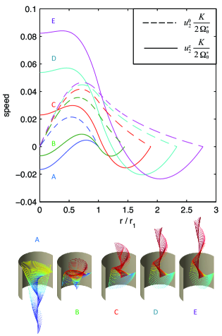
Figure 2: Top: Non-dimensional velocities for $l=1$, $\tan{(\alpha)=1.21}$ and $Kr_{1}=1.84$ for progressively increased cavity geometrical proportions $r_{0}/r_{1}=$ [1(A) 1.44(B) 1.89(C) 2.33(D) 2.78(E)]. Axial velocity is represented by solid lines and the azimuthal component by the dashed ones. Bottom: Flow streamlines. Colors are indicative of the speed magnitude along $u_{2}^{z}$: extrema are represented by the most intense colors, red for positive and blue for negative.

III Repeller and attractor vortices

It is commonly accepted that Eckart’s streaming is the result of pseudo-momentum transfer from the sound wave to the fluid Piercy and Lamb (1954). Consequently, the acoustic beam ($r<r_{1}$) should push the fluid away from the transducer. This is what actually occurs in weakly confined geometry, that is to say for the largest ratios $r_{0}/r_{1}$ (see Fig. 2 C to E). In these cases, confinement and mass conservation impose a back-flow at the periphery of the acoustic beam, resulting in azimuthal vorticity similar to the one observed by Eckart. But Bessel beams also carry an angular momentum, which is transmitted to the fluid and results in axial vorticity Anhauser et al. (2012). Since for $l>0$ the wave is rotating in the positive direction (when time increases, equiphase is obtained for growing $\theta$), the azimuthal velocity is also positive.

However, this analysis doesn’t hold when applied to very confined geometries such as A and B, where the beam covers almost all the cylindrical channel. Under these conditions, radial variations of the beam intensity must be considered. Indeed, in figure (1) we clearly see that the Bessel beam offers a shadow-area in the neighborhood of its axis, where the wave amplitude cancels. This holds for all non-zero orders vortices. The backflow generally appears where the wave forcing is weaker. Hence, the fluid recirculation can either occur near the walls or at the core of the beam, which becomes the only option as the free-space at the periphery of the vortex shrinks to 0, as in case A. Let’s call these vortices attractor vortices since they tend to drive fluid particles towards the sound source, and their opposite repeller vortices, since they push fluid particles away from the source. Although streaming pushing the fluid away from a transducer is common, (i) it is not usually associated with axial vorticity and (ii) the vorticity topology depends on the boundary conditions. Furthermore Bessel beams enable for the first time the synthesis of attractive vortices, offering original prospects for flow control and particle sorting in confined geometries.

Intrigued by this reverse-flow motion, we performed a systematic investigation on the conditions of its appearance. Looking at the expression of the velocity, we notice that the sign of $u_{2}^{z}(r=0)$ is independent of $\tan(\alpha)$, such that the set of parameters reduces to the topological charge $l$, the typical dimension $Kr_{1}$ and the geometrical ratio $r_{0}/r_{1}$. All these parameters were gathered in figure (3) to give an overview of the streaming induced by Bessel beams in confined space.

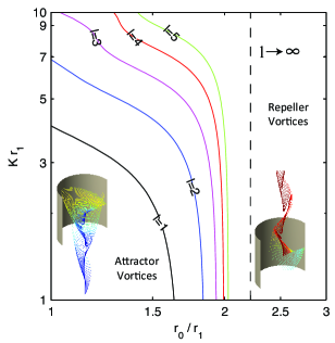
Figure 3: Contour plot of $u^{z}_{2}(r=0)=0$ at various topological charge $l$, typical dimension $Kr_{1}$ and geometrical ratio $r_{0}/r_{1}$. Parameters plane is partitioned into two areas, one close to the origin corresponding to attractor vortices with negative axial velocities at $r=0$ and the other one corresponding to repeller vortices. The dashed line at $r_{0}/r_{1}\sim 2.218$ indicates an asymptotic limit obtained for large $l$ values.

Looking at the flow map for $l=1$, we first notice that there is a bounded set of parameters leading to attractor vortices. Indeed, these vortices are squeezed by two restrictions: the beam must be confined enough (ratio $r_{0}/r_{1}$ close to one) as previously explained, and the value of $Kr_{1}$ has to be small. Looking back at figure (1.b), we notice that as $Kr_{1}$ increases, the Bessel function amplitude decreases on the periphery which facilitates the flow recirculation close to the channel walls. This trend is reinforced by the apparition of new nodes of the Bessel function for higher values of $Kr_{1}$ and the quadratic dependence of the streaming flow. In addition, as the beam gets wider, the envelope of the beam weakens for increasing $r$ and hence, the recirculation preferentially flows towards the periphery.

Introducing the topological order $l$ as a free parameter, we notice the progressive broadening of the attractor domain. Referring to figure (1.b), it appears that Bessel functions of higher order roughly translate towards increased $Kr_{1}$, or reciprocally need a higher $Kr_{1}$ to reach the analog extremum. This explains the $Kr_{1}$ part of the broadening, whereas the $r_{0}/r_{1}$ is due to the progressive flattening of Bessel functions, which nonetheless rapidly saturates. Using the asymptotic forms of Bessel development, we computed this limit in the appendix. The extreme value is given solving the equation $\ln(x)=1-1/x^{2},\quad\mbox{with}\quad x=r_{0}/r_{1}$. The existence of this upper bound highlights the essential condition of the confined nature of the channel.

To compute these last results, we use a window function, $A(s)$, with a sharp cut-off to ease the comparison with Eckart results. If we relax this condition, no change is expected in the case of weakly confined beams, $Kr_{1}>>1$. For such beam, the flow will recirculate preferentially at the periphery due to the radial decreasing of the Bessel function. The strictly confined case $r_{0}/r_{1}=1$ is possible since Bessel beams are the modes of cylindrical wave guides for discrete values of the radial wave number $K=s/r$, i.e no window A(s) is required. Hence flow reversal at the vortex core should be observable. The intermediate situation of strongly confined beam, $1<r_{0}/r_{1}=1<2$, is more challenging to carry out experimentally due to diffraction spreading. However, this problem is mitigated since truncated Bessel beam are weakly diffracting Durnin et al. (1987).

IV Conclusion

In this paper, we derive the streaming flow induced by Bessel beams (acoustical vortices). The resulting flow topology is reminiscent of cyclones with both axial and azimuthal vorticity. The axial component is solely controlled by the acoustic field. Regarding the azimuthal vorticity, two categories of flow pattern should be distinguished: repeller and attractor vortices. The first category exhibits a positive velocity at the center of the beam, and appears when the beam radius is small compared to the fluid cavity; whereas the latter needs a very confined geometry, and develops negative velocity in its core. To the best of our knowledge, streaming-based attractor beams have never been described before and are due to the specific radial dependence of the sound wave intensity in Bessel beams. This work opens prospects for vorticity control, which is an essential feature in many fluidic systems Ottino (1989); Chorin (1994); Gmelin and Rist (2001); Zhu et al. (2002). Moreover, the combination of attractive streaming and radiation pressure Baresh et al. (2013); Settnes and Bruus (2012); Zhang and Marston (2011) induced by acoustical vortices could provide an efficient method for particles sorting. Indeed, large particles are known to be more sensitive to radiation pressure and small particles to the streaming Hagsäter et al. (2007). Large particles would therefore be pushed away from the sound source by the radiation pressure while small particles would be attracted by the flow toward it. Compared to existing techniques relying on radiation pressure generated by standing waves Petersson et al. (2005); Wood et al. (2008), the advantage would be that a resonant cavity is not mandatory to sort particles with acoustical vortices since progressive waves can be used.

Appendix A Resolution of Eckart equation for acoustical vortices

Eckart acoustic streaming Eckart (1948) is adequately described by a set of non-linear partial differential equations. Although exact analytical solutions have not been found in the general case, the problem can be solved with a perturbation analysis, as long as the acoustic wave propagation is weakly nonlinear (weak acoustical Mach Number) and the flow remains laminar (weak Reynolds number). Following Eckart, the flow generated by a transducer can be decomposed into a first order compressible and irrotational flow (corresponding to the propagating acoustic wave) and a second order incompressible vortical flow (corresponding to the acoustic streaming) :

$$\rho = \rho_{0}+\rho_{1}+\rho_{2}+...$$ (12)

$$\vec{u} = \vec{u}_{1}+\vec{u}_{2}+...$$ (13)

with $\rho_{2}\ll\rho_{1}\ll\rho_{0}$ and $\|\vec{u_{2}}\|\ll\|\vec{u_{1}}\|$. Basically the order of magnitude of the ratio between first order and second order fields is given by the acoustical Mach number. In this development, we have considered a homogeneous fluid at rest in the absence of the acoustic field. Thus the density $\rho_{0}$ is constant in space and time, and the velocity $\vec{u_{0}}=\vec{0}$.

By replacing this decomposition into Navier-Stokes compressible equations, Eckart showed that the first order field is solution of D’Alembert (wave) equation. Acoustical vortices are solution of this equation in cylindrical coordinates D. and Dholakia (2005) and their expression calculated by Hefner and Marston Hefner and Marston (1999) takes the following form for weakly attenuated waves :

$$\rho_{1}(r,\theta,z,t)=\hat{\rho}_{1}A(Kr)J_{l}(Kr)\sin(l\theta+k_{z}z-\omega t)$$ (14)

In this equation, $\phi=l\theta+k_{z}z-\omega t$ is the phase of the acoustical vortex, $l$ the topological charge of the vortex, $\theta$ the angular coordinate, $k_{z}$ the projection of the wave vector on $z$-axis, $z$ the height, $\omega$ the wave frequency, $t$ the time. Finally, $\hat{\rho_{1}}$ is the amplitude of the first order density fluctuation, which is related to its pressure counterpart $\hat{P}_{1}$ according to $\hat{\rho_{1}}=\hat{P_{1}}/c^{2}$ and $K$ the transversal component of the wave vector. It is defined by the dispersion relation of an acoustical vortex: $K^{2}+k_{z}^{2}=\omega^{2}/c^{2}$, with $c$ the sound speed.

Eckart obtained in his paper a diffusion equation for the second order vorticity field $\vec{\varOmega}_{2}=\vec{\nabla}\times\vec{u}_{2}$, which can be used to compute the acoustic streaming. In the following, we consider steady streaming generated by a monochromatic acoustic wave with constant amplitude and therefore Eckart equations reduces to:

$$\Delta\vec{\varOmega_{2}} = -\frac{b}{\rho_{0}^{2}}\vec{\nabla}\rho_{1}\times\vec{\nabla}\frac{\partial\rho_{1}}{\partial t}$$ (15)

$$b = 4/3+\mu^{\prime}/\mu$$ (16)

with $\mu$ the shear viscosity and $\mu^{\prime}$ the bulk viscosity. From now on, we will use the shorthand notation $s=Kr$, and $s_{1}=Kr_{1}$, $s_{0}=Kr_{0}$. Besides, we introduce $B$ to gather the radial dependence of the beam:

$$B(s)=A(s)J_{l}(s)\\$$ (17)

where the function, $A(s)$, is introduced to limit the infinite lateral extension of Bessel function.The derivation of $\rho_{1}$ in equation (14) in cylindrical coordinates, and the replacement of the result into equation (15) gives a inhomogeneous Poisson equation with the first order field playing the role of the streaming source term:

$$\frac{1}{K^{2}}\Delta\vec{\varOmega}_{2}(r,\theta,z)=\varOmega_{\theta}^{\star}\frac{dB^{2}(s)}{ds}\vec{e_{\theta}}-\frac{\varOmega_{z}^{\star}}{s}\frac{dB^{2}(s)}{ds}\vec{e_{z}}$$ (18)

$$\varOmega_{\theta}^{\star}=\frac{1}{2}\frac{k_{z}\omega b}{K\rho_{0}c^{2}}E_{1}$$ (19)

$$\varOmega_{z}^{\star}=\frac{1}{2}\frac{\omega bl}{\rho_{0}c^{2}}E_{1}$$ (20)

$$E_{1}=c^{2}\frac{{\hat{\rho}_{1}}^{2}}{\rho_{0}}$$ (21)

The beam is assumed to be of infinite extent along $z$ and invariant by rotation $\theta$ around this axis, therefore $\vec{\varOmega}_{2}$ has only a radial dependence. Besides, the conservative nature of vorticity allows us to drop-off the $\vec{e_{r}}$ component. The resulting solution candidate for $\vec{\varOmega}_{2}$ is:

$$\vec{\varOmega}_{2}=\varOmega_{2}^{\theta}(s)\vec{e_{\theta}}+\varOmega_{2}^{z}(s)\vec{e_{z}}$$ (22)

Plugging it into equation (18) gives two linear ODEs:

$$s^{2}\frac{d^{2}}{ds^{2}}\varOmega_{2}^{\theta}+s\frac{d}{ds}\varOmega_{2}^{\theta}-\varOmega_{2}^{\theta}=s^{2}\varOmega_{\theta}^{\star}\frac{dB^{2}(s)}{ds}$$ (23)

$$s\frac{d^{2}}{ds^{2}}\varOmega_{2}^{z}+\frac{d}{ds}\varOmega_{2}^{z}=-\varOmega_{z}^{\star}\frac{dB^{2}(s)}{ds}$$ (24)

Using standard methods, the homogeneous ($H$) and particular ($P$) solutions are determined:

$${\varOmega_{2}^{\theta}}|_{H}=M_{1}^{\theta}s+\frac{N_{1}^{\theta}}{s}$$ (25)

$${\varOmega_{2}^{\theta}}|_{P}=\frac{1}{s}\varOmega_{\theta}^{\star}\int_{0}^{s}x_{1}B^{2}(x_{1})dx_{1}$$ (26)

The equation along $z$ is treated by introducing $g=\frac{d}{ds}\varOmega_{2}^{z}$

$$g|_{H} = \frac{M_{z}^{1}}{s}$$ (28)

$$g|_{P} = -\varOmega_{z}^{\star}\frac{B^{2}(s)}{s}$$ (29)

$$\varOmega_{2}^{z} = N_{1}^{z}+M_{z}^{1}\ln(s)-\varOmega_{z}^{\star}\int_{0}^{s}\frac{B^{2}(x_{1})}{x_{1}}dx_{1}$$ (30)

Removing the terms diverging at $s=0$, we have:

$$\vec{\varOmega}_{2} = \left[M_{1}^{\theta}s+\frac{1}{s}\varOmega_{\theta}^{\star}\int_{0}^{s}x_{1}B^{2}(x_{1})dx_{1}\right]\vec{e_{\theta}}$$ (32)

$$+\left[N_{1}^{z}-\varOmega_{z}^{\star}\int_{0}^{s}\frac{B^{2}(x_{1})}{x_{1}}dx_{1}\right]\vec{e_{z}}$$

Since the second order flow (streaming) is incompressible, we can introduce the vector potential $\vec{\Psi}_{2}$ verifying $\vec{u}_{2}=\vec{\nabla}\times\vec{\Psi}_{2}$ with the gauge $\vec{\nabla}.\vec{\Psi}_{2}=0$ to compute the velocity field from the vorticity field:

$$\Delta\vec{\Psi}_{2}=-\vec{\varOmega_{2}}$$ (33)

For symmetry reasons, the flow is assumed to be invariant by rotation $\theta$ around $z$ and translation along the propagation axis $z$, and due to the conservative nature of $\vec{u}_{2}$, the radial component is dropped off. Consequently, the velocity field is of the form: $\vec{u}_{2}=u_{2}^{\theta}(s)\vec{e_{\theta}}+u_{2}^{z}(s)\vec{e_{z}}$. Computing the curl of $\vec{\Psi}$ in order to get $\vec{u}_{2}$, we notice that $\vec{\Psi}_{2}=\Psi_{\theta}(s)\vec{e_{\theta}}+\Psi_{z}(s)\vec{e_{z}}$. Equation (33) is very similar to (15), except the source term:

$$s^{2}\Psi_{\theta}^{\prime\prime}+s\Psi_{\theta}^{\prime}-\Psi_{\theta}=-\frac{1}{K^{2}}\left(M_{1}^{\theta}s^{3}+s\varOmega_{\theta}^{\star}\int_{0}^{s}x_{1}B^{2}(x_{1})dx_{1}\right)$$

$$s\Psi_{z}^{\prime\prime}+\Psi_{z}^{\prime}=\frac{s}{K^{2}}\left(-N_{1}^{z}+\varOmega_{z}^{\star}\int_{0}^{s}\frac{B^{2}(x_{1})}{x_{1}}dx_{1}\right)$$

Using the same procedure as for $\vec{\varOmega}_{2}$ we get the general solution:

$$\Psi_{\theta} = M_{\theta}^{2}s-\frac{1}{K^{2}}\left(\frac{M_{1}^{\theta}}{8}s^{3}+\frac{\varOmega_{\theta}^{\star}I_{\theta}(s)}{s}\right)$$ (34)

$$\Psi_{z} = N_{z}^{2}+\frac{1}{K^{2}}\left(-N_{1}^{z}\frac{s^{2}}{4}+\varOmega_{z}^{\star}I_{z}(s)\right)$$ (35)

$$I_{\theta} = \int_{0}^{s}x_{3}\int_{0}^{x_{3}}\frac{1}{x_{2}}\int_{0}^{x_{2}}x_{1}B^{2}(x_{1})dx_{1}dx_{2}dx_{3}$$ (36)

$$I_{z} = \int_{0}^{s}\frac{1}{x_{3}}\int_{0}^{x_{3}}x_{2}\int_{0}^{x_{2}}\frac{B^{2}(x_{1})}{x_{1}}dx_{1}dx_{2}dx_{3}$$ (37)

The resulting velocity field can now be simply obtained by taking the curl of $\vec{\Psi_{2}}$:

$$u_{2}^{\theta} = \frac{1}{K}\left(\frac{1}{2}N_{1}^{z}s-\frac{1}{s}\varOmega_{z}^{\star}\varLambda^{l}_{\theta}(s)\right)$$ (38)

$$u_{z}^{(2)} = 2M_{\theta}^{2}K-\frac{1}{K}\left(\frac{M_{1}^{\theta}}{2}s^{2}+\varOmega_{\theta}^{\star}\varLambda^{l}_{z}(s)\right)$$ (39)

$$\varLambda^{l}_{\theta}(s) = \int_{0}^{s}x_{2}\int_{0}^{x_{2}}\frac{B^{2}(x_{1})}{x_{1}}dx_{1}dx_{2}$$ (40)

$$\varLambda^{l}_{z}(s) = \int_{0}^{s}\frac{1}{x_{2}}\int_{0}^{x_{2}}x_{1}B^{2}(x_{1})dx_{1}dx_{2}$$ (41)

This velocity field must satisfy the adherence boundary condition at the wall of the channel $s=s_{0}$:

$$u_{2}^{\theta}(s_{0}) = 0$$ (42)

$$u_{2}^{z}(s_{0}) = 0$$ (43)

Besides, the steady and incompressible nature of the flow must not violate mass conservation, such that a closure condition is enforced:

$$\begin{array}[]{llcr}&\int_{0}^{2\pi}\int_{0}^{r_{0}}\rho_{0}u_{2}^{z}(r)rdrd\theta&=&0\\ \Leftrightarrow&\int_{0}^{s_{0}}x_{1}u_{z}(x_{1})dx_{1}&=&0\end{array}$$ (44)

The determinant of the system is equal to $\frac{s_{0}^{4}}{8K}$, such that it always admits a unique solution. Solving this linear system of equations, we get:

$$N_{1}^{z} = \frac{2\varOmega_{z}^{\star}}{{s_{0}}^{2}}\varLambda^{l}_{\theta}(s_{0})$$ (45)

$$M_{\theta}^{1} = \frac{4\varOmega_{\theta}^{\star}}{{s_{0}}^{2}}\left(f(s_{0})-\frac{1}{2}\varLambda^{l}_{z}(s_{0})\right)$$ (46)

$$M_{\theta}^{2} = \frac{\varOmega_{\theta}^{\star}}{K^{2}}f(s_{0})$$ (47)

$$f(s) = -\frac{1}{2}\varLambda^{l}_{z}(s)+\frac{2}{s^{2}}\int_{0}^{s}x_{1}\varLambda^{l}_{z}(x_{1})dx_{1}$$ (48)

Including these boundary conditions in the expressions of the velocity field, we finally obtain:

$$u_{2}^{\theta}=\frac{\varOmega_{z}^{\star}}{K}\left(\frac{s}{{s_{0}}^{2}}\varLambda^{l}_{\theta}(s_{0})-\frac{1}{s}\varLambda^{l}_{\theta}(s)\right)$$

$$u_{z}^{(2)}=2\frac{\varOmega_{\theta}^{\star}}{K}\left(\left(1-\frac{s^{2}}{{s_{0}}^{2}}\right)f(s_{0})+\frac{1}{2}\left(\frac{s^{2}}{{s_{0}}^{2}}\varLambda^{l}_{z}(s_{0})-\varLambda^{l}_{z}(s)\right)\right)$$

Appendix B Asymptotic development when $Kr_{0}<<2\sqrt{l+1}$

In this section, we compute an asymptotic development of our final expression when $Kr_{0}<<2\sqrt{l+1}$. We show that Eckart’s result obtained for plane wave can be recovered as an asymptotic limit of our more general expression. Recovering, the Eckart result dictates the choice of the function $A(s)$:

$$A(s)=\begin{cases}1,\mbox{if }s<s_{1}\\ 0,\mbox{if }s\geqslant s_{1}\end{cases}$$ (49)

B.1 Asymptotic development

For all $s<s_{0}=Kr_{0}$, we have:

$$J_{l}(s)\sim\frac{1}{l!}\,{\left(\frac{s}{2}\right)}^{l}$$ (50)

$$\Lambda^{l}_{z}(s)\sim\begin{cases}\frac{{s}^{2\,l+2}}{{\left(2\,l+2\right)}^{2}\,{2}^{2\,l}\,{l!}^{2}},&\mbox{if }s<s_{1}\\ {s_{1}}^{2\,l+2}\,\frac{1+(2l+2)\mathrm{ln}\left(s\right/s_{1})}{\left(2\,l+2\right)^{2}\,{2}^{2\,l}\,{l!}^{2}},&\mbox{if }s\geqslant s_{1}\end{cases}$$ (51)

$$f\sim\begin{cases}\frac{{s}^{2\,l+2}}{{\left(2\,l+2\right)}^{2}\,\left(2\,l+4\right)\,{2}^{2\,l}\,{l!}^{2}}(2-\frac{2l+4}{2}),&\mbox{if }s<s_{1}\\ \\ C_{l}\left[\begin{array}[]{l}(s_{1}/s)^{2}\left(l\,(1-(s/s_{1})^{2}\,)+\frac{1}{l+2}\right)\\ +\left((l+1)\mathrm{ln}\left(s\right/s_{1})-(1/2)\right)\end{array}\right],&\mbox{if }s\geqslant s_{1}\end{cases}$$ (52)

$$\mbox{with}C_{l}=\frac{{s_{1}}^{2\,l+2}\,}{\left(2\,l+2\right)^{2}\,{2}^{2\,l}\,{l!}^{2}}$$ (53)

B.2 Recovering Eckart’s streaming with $l=0$ and $Kr_{0}<<1$

The case of plane wave can be recovered from our expression by considering a topological charge equal to zero and a radius $r_{0}\ll 1/K$:

$$\Lambda^{l}_{z}(s)\sim\begin{cases}s^{2}/4,&\mbox{if }s<s_{1}\\ (s_{1}^{2}/4)(1+2\mathrm{ln}\left(s\right/s_{1})),&\mbox{if }s\geqslant s_{1}\end{cases}$$ (54)

$$f\sim\begin{cases}0,&\mbox{if }s<s_{1}\\ \\ (s_{1}^{2}/8)\left[(s_{1}/s)^{2}+2\mathrm{ln}\left(s\right/s_{1})-1\right],&\mbox{if }s\geqslant s_{1}\end{cases}$$ (55)

In the original paper Eckart (1948), Eckart introduces the notation $x=s/s_{0}$ and $y=s_{1}/s_{0}$

$$u_{2}^{z}\sim 2\frac{\varOmega^{\star}_{\theta}}{K}\begin{cases}s_{1}^{2}/4\left[(1/2)(1-(x/y)^{2})-(1-y^{2}/2)(1-x^{2})-\ln(y)\right],&\mbox{if }s<s_{1}\\ \\ -s_{1}^{2}/4\left[(1-y^{2}/2)(1-x^{2})+\ln(x)\right],&\mbox{if }s\geqslant s_{1}\end{cases}$$ (56)

Equation (56) is exactly the expression of the acoustic streaming obtained by Eckart Eckart (1948) for plane waves.

B.3 Asymptotic limit for large values of $l$ and $Kr_{0}<<2\sqrt{l+1}$

$$\Lambda^{l}_{z}(s)\sim\begin{cases}\frac{{s}^{2\,l+2}}{{\left(2\,l\right)}^{2}\,{2}^{2\,l}\,{l!}^{2}},&\mbox{if }s<s_{1}\\ {s_{1}}^{2\,l+2}\,\frac{\mathrm{ln}\left(s\right/s_{1})}{\left(2\,l\right)\,{2}^{2\,l}\,{l!}^{2}},&\mbox{if }s\geqslant s_{1}\end{cases}$$ (57)

$$f\sim\begin{cases}-\frac{{s}^{2\,l+2}}{2{\left(2\,l\right)}^{2}\,{2}^{2\,l}\,{l!}^{2}},&\mbox{if }s<s_{1}\\ C_{l}\left[\begin{array}[]{l}(s_{1}/s)^{2}(1-(s/s_{1})^{2})\\ +\mathrm{ln}\left(s\right/s_{1})\end{array}\right],&\mbox{if }s\geqslant s_{1}\end{cases}$$ (58)

$$C_{l}=\frac{{s_{1}}^{2\,l+2}\,}{4l\,{2}^{2\,l}\,{l!}^{2}}$$ (59)

$$u_{2}^{z}(s=0)=2\frac{\varOmega^{\star}_{\theta}}{K}f(s_{0})$$ (60)

Using Eckart Eckart (1948) notation $y=s_{1}/s_{0}$:

$$u_{2}^{z}(s=0)=2\frac{\varOmega^{\star}_{\theta}C_{l}}{K}\left(y^{2}-1-\ln(y)\right)$$ (62)

We highlight here that in equation (62) $C_{l}$ is decreasing extremely fast such that increasing $l$ dramatically decreases the magnitude of $u_{2}^{z}(0)$.

References

- Kumar et al. (2007) A. Kumar, P. Gogate, and A. Pandit, Ind. Eng. Chem. Res. 46, 4368 (2007).
- Gale and Busnaina (1999) G. Gale and A. Busnaina, Part. Sci. and Techn.: An Int. J. 17, 229 (1999).
- Li et al. (2004) X. Li, Y. Yang, and W. Cheng, J. Mat. Sci. 39, 3211 (2004).
- Muller et al. (2012) P. Muller, R. Barnkob, M. Jensen, and H. Bruus, Lab Chip 22, 4617 (2012).
- Baker et al. (2001) K. Baker, V. Robertson, and F. Duck, Phys. Ther. 81, 1351 (2001).
- Crum (2006) L. Crum, J. Acoust. Soc. Am. 117, 2350 (2006).
- Wiklund (2012) M. Wiklund, Lab Chip 12, 2438 (2012).
- Friend and Yeo (2011) J. Friend and L. Yeo, Review of Modern Physics 83, 647 (2011).
- Yeo and Friend (2014) L. Yeo and J. Friend, Ann. Rev. Fluid Mech. 46, 379 (2014).
- Wixforth et al. (2004) A. Wixforth, C. Strobl, C. Gauer, A. Toegl, J. Scriba, and Z. Guttenberg, Anal. Bioanal. Chem. 379, 982 (2004).
- Renaudin et al. (2006) A. Renaudin, P. Tabourier, V. Zang, J. Camart, and C. Druon, Sensors and Actuators B 113, 389 (2006).
- Brunet et al. (2010) P. Brunet, M. Baudoin, O. Matar, and F. Zoueshtiagh, Phys. Rev. E 81, 036315 (2010).
- Qi et al. (2008) A. Qi, L. Yeo, and J. Friend, Phys. Fluids 20, 074103 (2008).
- Shiokawa et al. (1990) S. Shiokawa, Y. Matsui, and T. Ueda, Jpn. J. Appl. Phys. 29, 137 (1990).
- Tan et al. (2009) M. Tan, J. Friend, and L. Yeo, Phys. Rev. Lett. 103, 024501 (2009).
- Baudoin et al. (2012) M. Baudoin, P. Brunet, O. Matar, and E. Herth, Appl. Phys. Lett. 100, 154102 (2012).
- Blamey et al. (2013) J. Blamey, L. Yeo, and J. Friend, Langmuir 29, 3835 (2013).
- Sritharan et al. (2006) K. Sritharan, C. Strobl, M. Schneider, and A. Wixforth, Appl. Phys. Lett. 88, 054102 (2006).
- Frommelt et al. (2008) T. Frommelt, M. Kostur, M. Wenzel-Schäfer, P. Talkner, P. Hänggi, and A. Wixforth, Phys. Rev. Lett. 100, 034502 (2008).
- Beyer (1997) R. Beyer, Nonlinear Acoustics (Acoust. Soc. Am., 1997).
- Riley (2001) N. Riley, Ann. Rev. Fluid Mech. 33, 43 (2001).
- Hamilton (2003) M. Hamilton, J. Acoust. Soc. Am. 113, 153 (2003).
- Schlichting (1932) H. Schlichting, Phys. Zeitung 33, 327 (1932).
- Rayleigh (1884) L. Rayleigh, Ph. Trans. Roy Soc. London 175, 1 (1884).
- Eckart (1948) C. Eckart, Phys. Rev. 73, 68 (1948).
- Piercy and Lamb (1954) J. Piercy and J. Lamb, Proc. Roy. Soc. London. A 226, 43 (1954).
- Sato and Fujii (2001) M. Sato and T. Fujii, Phys. Rev. E 64, 026311 (2001).
- Rudenko and Soluyan (1971) O. Rudenko and S. Soluyan, Akust. Zh. 17, 122 (1971).
- Rudenko and Sukhorukov (1998) O. Rudenko and A. Sukhorukov, Acoustical Physics 44, 565 (1998).
- Sou et al. (2011) I. Sou, J. Allen, C. Layman, and C. Ray, Exp. Fluids 51, 1201 (2011).
- Romanenko (1960) E. Romanenko, Sov. Phys. Acoustics (1960).
- Statnikov (1967) Y. Statnikov, Sov. Phys. Acoustics 13, 122 (1967).
- Menguy and Gilbert (1999) L. Menguy and J. Gilbert, J. Acoust. Soc. Am. 105, 958 (1999).
- I. et al. (2013) R. I., V. Daru, H. Baillet, S. Moreau, J. Valiere, D. Baltean-Carles, and C. Weisman, J. Acoust. Soc. Am. 134, 1791 (2013).
- Nyborg (1998) W. Nyborg, “Nonlinear acoustics,” (Academic Press, 1998) Chap. 7.
- Thomas et al. (2010) J.-L. Thomas, T. Brunet, and F. Coulouvrat, Phys. Rev. E 81, 016601 (2010).
- Allen et al. (1992) L. Allen, M. Beijersbergen, R. Spreeuw, and J. Woerdman, Phys. Rev. A 45, 8185 (1992).
- Durnin et al. (1987) J. Durnin, M. J.J., and J. Eberly, Phys. Rev. Lett. 58, 1499 (1987).
- Hefner and Marston (1999) B. Hefner and P. Marston, J. Acoust. Soc. Am. 106, 3313 (1999).
- Thomas and Marchiano (2003) J.-L. Thomas and R. Marchiano, Phys. Rev. Lett. 91, 244302 (2003).
- Marchiano and Thomas (2008) R. Marchiano and J.-L. Thomas, Phys. Rev. Lett. 101, 064301 (2008).
- Brunet et al. (2009) T. Brunet, J.-L. Thomas, R. Marchiano, and F. Coulouvrat, New J. Phys. , 013002 (2009).
- He et al. (1995) H. He, M. Friese, N. Heckenberg, and H. Rubinsztein-Dunlop, Phys. Rev. Lett. 75, 826 (1995).
- Volke-Sepulveda et al. (2008) J. Volke-Sepulveda, A. Santillan, and R. R. Boullosa, Phys. Rev. Lett. 100, 024302 (2008).
- Anhauser et al. (2012) A. Anhauser, R. Wunenburger, and E. Brasselet, Phys. Rev. Lett. 109, 034301 (2012).
- Ottino (1989) J. Ottino, The kinematics of mixing: stretching, chaos, and transport (Cambridge Texts in Applied Mathematics, 1989).
- Chorin (1994) A. Chorin, Vorticity and turbulence, Vol. 103 (Springer, 1994).
- Gmelin and Rist (2001) C. Gmelin and U. Rist, Phys. Fluids 13 (2001).
- Zhu et al. (2002) Q. Zhu, M. Wolfgang, D. Yue, and M. Triantafyllou, J. Fluid Mech. 468, 1 (2002).
- Baresh et al. (2013) D. Baresh, J.-L. Thomas, and R. Marchiano, J. Acoust. Soc. Am. 133, 25 (2013).
- Settnes and Bruus (2012) M. Settnes and H. Bruus, Phys. Rev. E 85, 016327 (2012).
- Zhang and Marston (2011) L. Zhang and P. Marston, Phys. Rev. E 84, 035601(R) (2011).
- Hagsäter et al. (2007) S. Hagsäter, T. Jensen, H. Bruus, and J. Kutter, Lab Chip 7, 1336 (2007).
- Petersson et al. (2005) F. Petersson, A. Nilsson, C. Holm, H. Jönsson, and T. Laurell, Lab on a Chip 5, 20 (2005).
- Wood et al. (2008) C. Wood, S. Evans, J. Wunningham, and R. O’Rorke, Appl. Phys. Lett. 92, 044104 (2008).
- Note (1) NB: In his seminal paper, Eckart also computed the irrotational part of the second order flow corresponding to the effect of nonlinearities on the acoustic wave propagation. Then, using Helmoltz decomposition, he focused on the incompressible part, corresponding to the acoustic streaming. Here we do not consider the effect of nonlinearities on the acoustic wave propagation.
- D. and Dholakia (2005) M. D. and K. Dholakia, Contemporary Physics 46, 15 (2005).