Fully coherent follow-up of continuous gravitational-wave candidates: an application to Einstein@Home results

Abstract

We characterize and present the details of the follow-up method used on the most significant outliers of the Hough Einstein@Home all-sky search for continuous gravitational waves Aasi et al. (2013a). This follow-up method is based on the two-stage approach introduced in Shaltev and Prix (2013), consisting of a semicoherent refinement followed by a fully coherent zoom. We quantify the efficiency of the follow-up pipeline using simulated signals in Gaussian noise. This pipeline does not search beyond first-order frequency spindown, and therefore we also evaluate its robustness against second-order spindown. We present the details of the Hough Einstein@Home follow-up Aasi et al. (2013a) on three hardware-injected signals and on the 8 most significant search outliers of unknown origin.

I Introduction

The search for unknown sources of continuous gravitational waves (CWs) is computationally bound due to the enormous parameter space that needs to be covered Brady and Creighton (2000). Advanced semicoherent search techniques, such as Cutler et al. (2005); Pletsch and Allen (2009), are typically used to identify interesting regions of the parameter space, which then require fully coherent follow-up studies in order to confirm or discard potential CW candidates. The parameter space associated with these candidates is substantially smaller than the original search space. However, it is still large enough to lead to a prohibitive computing cost, when data of order of months or years is analyzed fully coherently with a classical grid-based method Brady et al. (1998). Therefore, an alternative follow-up method was developed, which combines the $\mathcal{F}$-statistic Jaranowski et al. (1998)Cutler and Schutz (2005) with a Mesh Adaptive Direct Search (MADS) Audet and E (2004) algorithm. This allows us to fully coherently examine long data sets at a feasible computational cost Shaltev and Prix (2013).

In the present work we describe how the two-stage algorithm proposed in Shaltev and Prix (2013) was adapted to follow up the most significant outliers in the Hough S5 Einstein@Home search Aasi et al. (2013a). We first validate the follow-up pipeline by performing Monte-Carlo studies. We inject and search for simulated CW signals added into simulated Gaussian noise data. Then we show how the search method was applied to 35 outliers identified in the Einstein@Home search, 27 of which are associated with 3 simulated signals (hardware injections, discussed in Sec.V.1).

The paper is organized as follows. In Sec. II we briefly recap the Einstein@Home all-sky search for periodic gravitational waves in data from the fifth LIGO science run (S5). In Sec. III we summarize the two-stage follow-up method and introduce the search pipeline. The efficiency of the follow-up algorithm is tested with Monte-Carlo studies presented in Sec. IV. In Sec. V.1 we present the follow-up results for the 27 outliers associated with 3 hardware injections. In Sec. V.2 we show the results of the follow-up for the remaining CW outliers. Section VI presents a discussion of the results and concluding remarks.

Notation and conventions

When referring to a quantity $Q$ of the original Hough search, we denote it as $Q_{\mathrm{HS}}$. A quantity measured after the pre-refinement stage is denoted as $Q_{\mathrm{PR}}$, after the refinement as $Q_{\mathrm{R}}$, and as $\widetilde{Q}_{\mathrm{Z}}$ after the fully coherent zoom stage using all the data (consistent with the notation of Shaltev and Prix (2013)). We use an overbar ($\overline{Q}$) to denote an average over segments.

II The Hough S5 Einstein@Home all-sky search

The Einstein@Home all-sky search Aasi et al. (2013a) uses the semicoherent Hough-transform method Krishnan et al. (2004), which consists of dividing the entire data span into $N$ shorter segments of duration $\Delta T$. In a first step, a coherent $\mathcal{F}$-statistic search is performed on a coarse grid for each of the data segments. Then the Hough number-count statistic, defined in Eq. (6), is computed on a finer grid, using the $\mathcal{F}$-statistic values from the individual segments.

In this paper we focus on the S5R5 search of Aasi et al. (2013a), which spans approximately $264$ days of data from the Hanford (H1) and Livingston (L1) LIGO detectors. This dataset was divided into $N=121$ segments of duration $\Delta T=25$ hours each. The parameter space covered by this search spans the entire sky, a frequency range $f\in[50,1190]\ \mathrm{Hz}$, and a spindown range $\dot{f}\in[-20,1.1]\times 10^{-10}\ \mathrm{Hz}\ \mathrm{s}^{-1}$.

The phase evolution of the expected signal at the detector can be written as Jaranowski et al. (1998)

$$\Phi(t) \approx \Phi_{0}+2\pi\sum_{k=0}^{s}\frac{f^{(k)}(t_{0})(t-t_{0})^{k+1}}{(k+1)!}$$

$$+ 2\pi\frac{\mathbf{r}(t)}{c}\mathbf{n}\sum_{k=0}^{s}\frac{f^{(k)}(t_{0})(t-t_{0})^{k}}{k!}\ ,$$

where $\Phi_{0}$ is the initial phase, $f^{(k)}\equiv\frac{d^{k}f}{dt^{k}}$ represent the time derivatives of the signal frequency $f$ at the solar system barycenter (SSB) at reference time $t_{0}$, $s$ is the maximal considered spindown order, $c$ is the speed of light, and $\mathbf{r}(t)$ is the vector pointing from the SSB to the detector. The unit vector $\mathbf{n}\equiv(\cos\alpha\cos\delta,\sin\alpha\cos\delta,\sin\delta)$ points from the SSB to the CW source, where $\alpha,\,\delta$ are the standard equatorial coordinates referring to right-ascension and declination, respectively.

The $\mathcal{F}$-statistic is one of the standard coherent techniques used to extract the CW signals from the noisy detector data. This statistic is the result of matched-filtering the data with a signal template characterized by the phase-evolution parameters $\lambda\equiv\{\alpha,\delta,f,\dot{f}\}$. The amplitude parameters, namely, the intrinsic amplitude $h_{0}$, the inclination angle $\iota$, the polarization angle $\psi$ and the initial phase $\phi_{0}$ have been analytically maximized over Jaranowski et al. (1998). In a coherent grid-based $\mathcal{F}$-statistic search the number of templates increases with a high power of the observation time Prix (2007). Hence these searches are not suitable for wide parameter-space all-sky surveys. However, the reduction of the coherent baseline in a semicoherent search Brady and Creighton (2000); Cutler et al. (2005) makes these techniques computationally feasible in a distributed computing environment such as Einstein@Home, and (usually) more sensitive at fixed computing cost Prix and Shaltev (2012).

The template bank used to cover the parameter space is constructed using the notion of mismatch Balasubramanian et al. (1996); Owen (1996). This is defined as the fractional loss of squared signal-to-noise ratio (SNR) between a template $\lambda$ and the signal location $\lambda_{\mathrm{s}}$. We use the definition of SNR given in Jaranowski et al. (1998), and denote it as $\rho$.

To quadratic order in parameter-space offsets $\Delta\lambda^{i}\equiv\lambda^{i}-\lambda_{\mathrm{s}}^{i}$, the mismatch can be approximated by

$$\mu^{*}\equiv g_{ij}(\lambda_{\mathrm{s}})\Delta\lambda^{i}\Delta\lambda^{j}\,,$$ (2)

where $g_{ij}$ is a symmetric positive-definite matrix referred to as the parameter-space metric. The indices $i,j$ label the phase-evolution parameters, and we use summation convention over repeated indices. This metric mismatch $\mu^{*}$ can be interpreted as a distance measure in parameter space.

In the S5R5 analysis the templates at frequency $f$ were placed on a coarse grid constructed using the following spacings Aasi et al. (2013a):

$$d\theta_{\mathcal{F}}=\frac{\sqrt{3}\,c}{v_{d}f\Delta T},\quad df=\frac{\sqrt{12\,m}}{\pi\Delta T},\quad d\dot{f}=\frac{\sqrt{3.3\,m}}{\Delta T^{2}}\,,$$ (3)

where $d\theta_{\mathcal{F}}$ is the angular resolution of the coarse sky grid, $df,\,d\dot{f}$ are the frequency and spindown resolutions, respectively; $m$ is the nominal single-dimension mismatch, taken equal to $0.3$ in Aasi et al. (2013a), and $v_{d}$ is the Earth’s rotation speed at the equator. Due to limitations of the Einstein@Home environment on the memory footprint of the application, the spindown resolution was not increased for the fine grid. Instead the $d\dot{f}$-resolution of Eq. (3) was determined in a Monte-Carlo study so as to not significantly lose detection efficiency.

The resolution of the fine sky grid at frequency $f$ is given by Aasi et al. (2013a)

$$d\theta_{H}=\frac{c\,df}{\wp fv_{y}}\ ,$$ (4)

where $\wp$ is the pixel factor and $v_{y}$ is the Earth’s orbital velocity. With $\wp=0.5$, $m=0.3$ the sky refinement used in the S5R5 search yields $\mathcal{N}_{\mathrm{sky}}^{\mathrm{ref}}=(d\theta_{\mathcal{F}}/d\theta_{H})^{2}\approx 8444$ Aasi et al. (2013a).

Every parameter-space point of the search is assigned a significance, or critical ratio $(\mathrm{CR})$, value Aasi et al. (2013a):

$$\mathrm{CR}=\frac{n_{\mathrm{c}}-\bar{n}_{\mathrm{c}}}{\sigma}\ ,$$ (5)

with

$$n_{\mathrm{c}}=\sum_{\ell=1}^{N}w_{\ell}\,n_{\ell}$$ (6)

the Hough number count, where $w_{\ell}$ is the weight for segment $\ell$ at a frequency $f$ and a sky position $(\alpha,\delta)$; $n_{\ell}=1$ if the $\mathcal{F}$-statistic crosses a certain threshold value (namely $2\mathcal{F}>5.2$ in Aasi et al. (2013a)) otherwise $n_{\ell}=0$; $\bar{n}_{\mathrm{c}}$ and $\sigma$ are the expected value and the standard deviation of $n_{\mathrm{c}}$ in Gaussian noise. The candidates are ordered by their significance.

III Follow-up method

III.1 The modified two-stage follow-up

A slightly adapted version of the two-stage follow-up procedure Shaltev and Prix (2013) was used in Aasi et al. (2013a) and is presented here. As mentioned in Sec. II, the original Hough search did not use refinement in $\dot{f}$ and this led to a reduction in localization accuracy. To recover from this, we perform a pre-refinement by re-running the original Hough search with a finer grid around the outlier being followed up. Namely, we increase the resolution of the $\dot{f}$-grid by a factor $N=121$, and the sky-resolution by doubling the pixel factor $\wp$ in Eq. (4). The usefulness of this pre-refinement is illustrated in Fig. 1.

The loudest parameter-space point after pre-refinement provides the starting point for the subsequent MADS-based follow-up method described in Shaltev and Prix (2013): Namely, we first employ the semicoherent $\mathcal{F}$-statistic $\overline{2\mathcal{F}}$, defined as

$$\overline{2\mathcal{F}}(\lambda)\equiv\frac{1}{N}\sum_{\ell=1}^{N}2\mathcal{F}_{\ell}(\lambda)\,,$$ (7)

where $2\mathcal{F}_{\ell}(\lambda)$ is the coherent $\mathcal{F}$-statistic computed on segment $\ell$ at the parameter-space point $\lambda$. This is computed on the original Hough segments to further improve the localization of the maximum-likelihood parameter-space point, using the gridless MADS search method described in more detail in Shaltev and Prix (2013). This stage is called refinement, with detection statistic $\overline{2\mathcal{F}}_{\mathrm{R}}$ for the loudest resulting candidate.

Next we apply the so-called $\mathcal{F}$-statistic consistency veto of Aasi et al. (2013a); Keitel et al. (2014), namely

$$\text{veto if }\overline{2\mathcal{F}}_{\mathrm{R}}<\max\{\overline{2\mathcal{F}}^{\mathrm{H1}}_{\mathrm{R}},\,\overline{2\mathcal{F}}^{\mathrm{L1}}_{\mathrm{R}}\}\,,$$ (8)

where $\overline{2\mathcal{F}}_{\mathrm{R}}^{\mathrm{H1},\mathrm{L1}}$ denote the corresponding semicoherent $\mathcal{F}$-statistic values from the individual detectors H1 and L1, respectively.

Then, in the so-called zoom stage, we compute the fully-coherent $\widetilde{2\mathcal{F}}_{\mathrm{Z}}$ statistic using all the data. From this we determine whether the resulting candidate is consistent with the signal model or with Gaussian noise.

III.2 Classification of zoom outcomes

We distinguish three possible outcomes of the zoom stage:

• Consistency with Gaussian noise ($G$) - the fully coherent $\widetilde{2\mathcal{F}}_{\mathrm{Z}}$ value does not exceed a prescribed threshold, i.e.,

  $$\widetilde{2\mathcal{F}}_{\mathrm{Z}}<\widetilde{2\mathcal{F}}_{\mathrm{\mathrm{th}}}^{(G)}\,,$$ (9)

  where $\widetilde{2\mathcal{F}}_{\mathrm{\mathrm{th}}}^{(G)}$ is chosen to correspond to some (small) false-alarm probability $p_{\mathrm{fA}}$ in Gaussian noise. The single trial false-alarm probability for a given $\widetilde{2\mathcal{F}}_{\mathrm{\mathrm{th}}}^{(G)}$ threshold is $p_{\mathrm{fA}}^{1}=(1+\mathcal{F})e^{-\mathcal{F}}$ ( see, e.g., Shaltev and Prix (2013) for details). For example, we find that a threshold of $\widetilde{2\mathcal{F}}_{\mathrm{\mathrm{th}}}^{(G)}=90$ corresponds to a false-alarm probability $\sim\mathcal{O}(10^{-18})$ for a single template. Assuming $\mathcal{N}$ independent templates and $p_{\mathrm{fA}}\ll 1$, the false-alarm is $p_{\mathrm{fA}}\approx\mathcal{N}p_{\mathrm{fA}}^{1}$.

• Non-Gaussian origin ($\neg G$) - the candidate is loud enough to be inconsistent with Gaussian noise at the chosen $p_{\mathrm{fA}}$, i.e.,

  $$\widetilde{2\mathcal{F}}_{\mathrm{Z}}\geq\widetilde{2\mathcal{F}}_{\mathrm{\mathrm{th}}}^{(G)}\ .$$ (10)

• Signal recovery ($S$) - defined as a subclass of $\neg G$, namely a signal is considered recovered if for the final zoomed candidate the $\widetilde{2\mathcal{F}}_{\mathrm{Z}}$ value exceeds the Gaussian-noise threshold $\widetilde{2\mathcal{F}}_{\mathrm{\mathrm{th}}}^{(G)}$ and falls into a predicted signal interval:

  $$\widetilde{2\mathcal{F}}_{\mathrm{\mathrm{th}}}^{(S)}<\widetilde{2\mathcal{F}}_{\mathrm{Z}}<\widetilde{2\mathcal{F}}_{\mathrm{\max}}^{(S)}\ ,$$ (11)

  where $\widetilde{2\mathcal{F}}_{\mathrm{\mathrm{th}}}^{(S)}\equiv\max\{\widetilde{2\mathcal{F}}_{\mathrm{\mathrm{th}}}^{(G)},\,\widetilde{2\mathcal{F}}_{o}-n_{u}\,\sigma_{o}\}$, and $\widetilde{2\mathcal{F}}_{\mathrm{\max}}^{(S)}\equiv\widetilde{2\mathcal{F}}_{o}+n_{u}\,\sigma_{o}$, with expectation

  $$\widetilde{2\mathcal{F}}_{o}\approx 4+N\,\left(\overline{2\mathcal{F}}_{\mathrm{R}}-4\right)\,,$$ (12)

  and variance

  $$\sigma^{2}_{o}\approx 2\left(4+2N\,\left(\overline{2\mathcal{F}}_{\mathrm{R}}-4\right)\right)\,.$$ (13)

  The number $n_{u}$ determines the probability that a true signal candidate would fall into this interval. For example, $n_{u}=6$ corresponds roughly to a confidence of$~{}\sim 99.6\%$ (provided $G$ and $S$ are disjoint).

III.3 Choice of MADS parameters

In both stages the parameter space is explored on a dynamically created mesh by using a MADS-based algorithm Audet and E (2004). MADS itself is a general purpose algorithm for derivative-free optimization, which is typically applied to computationally expensive problems with unknown derivatives. The input to the MADS-based algorithm is a starting point $\lambda_{\mathrm{c}}$, a search bounding box $\Delta\lambda_{\mathrm{R}}$ around $\lambda_{\mathrm{c}}$ and a set of MADS parameters, which govern the choice of evaluation points, namely $\{d\lambda,u_{b},w^{+}_{\mathrm{min}},w^{+}_{\mathrm{max}},w^{-},p\}$, where $d\lambda$ is the initial step, $u_{b}$ is the mesh update basis, $w^{+}_{\mathrm{min}}$ and $w^{+}_{\mathrm{max}}$ are the mesh-coarsening exponents, $w^{-}$ denotes the mesh-refining exponent and $p$ is the maximum number of templates to search over; for details we refer the reader to Sec. IIIE in Shaltev and Prix (2013). The algorithm parameters for the MADS-based refinement and zoom stage are summarized in Table 1. These parameters have been found to yield good results in Monte-Carlo studies.

stage	$w^{-}$	$w^{+}_{\mathrm{min}}$	$w^{+}_{\mathrm{max}}$	$u_{b}$	$p$
R	-1	1	20	2	20000
Z	-1	1	50	1.2	20000

Table 1: Follow-up algorithm parameters for the refinement and zoom stage.

III.4 Follow-up parameter-space regions

We stress that the bounding box $\Delta\lambda_{\mathrm{R}}$ used for the refinement differs with respect to what is described in Shaltev and Prix (2013). There the refinement is restricted to the semicoherent metric ellipsoid centered on a candidate. Here, instead, the refinement stage is performed on a box that was empirically determined to be large enough to contain the true signal location with very high confidence:

$$\begin{split}\Delta\alpha=0.4\ \mathrm{rad}\,,&\quad\Delta\delta=0.4\ \mathrm{rad}\\ \Delta f=1\times 10^{-4}\ \mathrm{Hz}\,,&\quad\Delta\dot{f}=1\times 10^{-9}\ \mathrm{Hz}/\mathrm{s}\ .\end{split}$$ (14)

Given that this follow-up was not computationally limited, we did not attempt to find the smallest possible refinement region.

The zoom search is constrained by a Fisher ellipse scaled to 24 standard deviations, as described in Shaltev and Prix (2013). This large number was chosen empirically by increasing it until the pipeline performance did not further improve.

The minimal spindown order required is related to parameter-space thickness measured in terms of the extent of the metric ellipse along that direction Brady and Creighton (2000); Cutler et al. (2005); Prix and Shaltev (2012). As a rule of thumb, the maximal spindown order required in a search increases with the time spanned by the data. In the Hough Einstein@Home all-sky search Aasi et al. (2013a), the follow-up procedure did not include second-order spindown. In Secs. IV we show the performance of the follow-up pipeline on signals with zero second-order spindown, while in Sec. IV.3 we study the robustness of this method in the case of maximal second-order spindown (as considered in Aasi et al. (2013a)).

IV Monte-Carlo studies

(a)

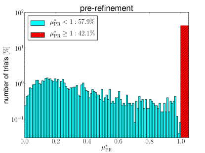
(b)

(c)

Figure 1: Semicoherent metric mismatch of the subset of 2500 injections with $\overline{\rho^{2}}\in{[5,6]}$ at different stages of the Monte-Carlo. The panel (a) shows the metric mismatch distribution after the original hierarchical search. The panel (b) shows the metric mismatch distribution after the pre-refinement stage. The panel (c) shows the metric mismatch distribution after the refinement stage. The hatched bar in each panel shows the percentage of trials with $\mu^{*}\geq 1$.

IV.1 Setup

We test the proposed follow-up pipeline in an end-to-end Monte-Carlo study using the LALSuite LAL (2011) software package. In particular we use the following LALApps applications: Makefakedata_v4 to generate Gaussian noise and inject CW signals; FstatMetric_v2 to compute the fully coherent or semicoherent metric; HierarchicalSearch for the semicoherent Hough-transform search; FStatSCNomad for the semicoherent $\mathcal{F}$-statistic optimization with MADS, and FStatFCNomad for the fully coherent $\mathcal{F}$-statistic MADS optimization, where for the MADS algorithm we use the reference implementation NOMAD Le Digabel (2011).

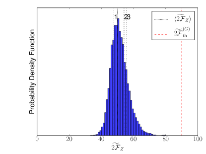
Figure 2: The figure shows the $\widetilde{2\mathcal{F}}_{\mathrm{Z}}$ distribution after the fully coherent 4-D $\{\alpha,\delta,f,\dot{f}\}$ zoom stage of 15000 searches in pure Gaussian noise data without injected signals. The maximum value is $\widetilde{2\mathcal{F}}_{\mathrm{Z}}^{\max}=$ 79.36 , and the mean value is $\langle\widetilde{2\mathcal{F}}_{\mathrm{Z}}\rangle=$ $51.40$ (dotted line). The labels 1,2,3 refer to the search outliers at roughly $434$, $677$ and $984$ Hz, respectively (see Tables 3). The vertical red line marks the noise threshold.

We apply the follow-up chain to 15000 different noise realizations with and without injected signals. The Gaussian noise realizations are generated with the MakeFakedata_v4 application using the same timestamps of the SFTs used in the original Einstein@Home search with detector noise level of $\sim 2\times 10^{-23}\,\mathrm{Hz}^{-1/2}$ per detector. The signal parameters are uniformly drawn in the ranges $\cos\iota\in[-1,1]$, $\psi\in[-\pi/4,\pi/4]$, $\phi_{0}\in[0,2\pi]$ and $f\in{[185,186]}\ \mathrm{Hz}$, and the sky position is drawn isotropically on the sky. The frequency range has been chosen in the most sensitive region of the LIGO detectors. The spindown value is randomly chosen in the range $\dot{f}\in(-\frac{f_{0}}{\tau_{0}},0.1\frac{f_{0}}{\tau_{0}})$ with minimal spindown age $\tau_{0}=800\ \mathrm{yr}$ at $f_{0}=50\ \mathrm{Hz}$. The signal amplitude is high enough such that the $\mathrm{SNR}^{2}$ in the point of injection is uniformly distributed in the range $\overline{\rho^{2}}\in[0,6]$.

We begin the end-to-end validation with a simulation stage of the original S5R5 Einstein@Home search by using the original search setup, i.e., the same frequency and spindown grid spacings given by Eq. (3). The S5R5 search has been partitioned in independent computing tasks, referred to as workunits (WUs). For a detailed discussion of the WU see Sec. III C in Aasi et al. (2013a). To save computing power, we do not rerun an entire WU in this simulation stage, but we center a search grid around a random point in the vicinity of the injected signal, searching over 10 frequency bins in total. The sky grid is constructed by extracting 16 points around the candidate from the original sky-grid file. However, this reduced parameter-space size is still sufficiently large to make possible the selection of candidates due to the noise, if the signal is weak as might happen in a real search, and not artificially select a point close to the true signal location.

In Fig. 1 we show the semicoherent metric mismatch distribution, computed with Eq. (2), after the Hough search, the pre-refinement Hough search and after the refinement stage. The loudest point selected from the refinement stage is used as a starting point for the fully coherent $\mathcal{F}$-statistic zoom search.

IV.2 Efficiency of the follow-up pipeline

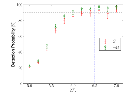
(a)

(b)

Figure 3: Monte-Carlo study of the efficiency of the follow-up pipeline. The panel (a) shows the percentage of the injected signals without second-order spindown classified as recovered ($-$ $\ S$), and with a non-Gaussian origin (${\color[rgb]{0,1,0}\times}\ \neg G$), as function of the average $2\mathcal{F}$ value of the candidate after the original semicoherent Hough-transform search ($\overline{2\mathcal{F}}_{\mathrm{c}}$). The panel (b) shows the percentage of the injected signals with second-order spindown classified as recovered ($-$ $\ S$), and with a non-Gaussian origin (${\color[rgb]{0,1,0}\times}\ \neg G$), as function of $\overline{2\mathcal{F}}_{\mathrm{c}}$. The error bars account for $95\%$ confidence level. The $90\%$ detection probability is marked with the horizontal dashed line. The vertical dotted line denotes the $2\mathcal{F}$ threshold used to select candidates in Aasi et al. (2013a).

We first apply the follow-up pipeline to Gaussian noise data without any injected signals. This is required to ensure the applicability of the threshold $\widetilde{2\mathcal{F}}_{\mathrm{\mathrm{th}}}^{(G)}=90$ used to consider a candidate as conform with the Gaussian noise hypothesis. The distribution of the $\widetilde{2\mathcal{F}}_{\mathrm{Z}}$ values is plotted in Fig. 2. The maximal value found is $\widetilde{2\mathcal{F}}_{\mathrm{Z}}^{\max}=79.36$, which is well below the $\neg G$ treshold of $\widetilde{2\mathcal{F}}_{\mathrm{\mathrm{th}}}^{(G)}=90$.

In Fig. 3a we plot the percentage of the injected signals classified as recovered ($S$), and as of non-Gaussian origin ($\neg G$), as a function of the average $2\mathcal{F}$ value of the candidate after the simulation stage. We are able to distinguish $\geq 90\,\%$ of the candidates from Gaussian noise above $\overline{2\mathcal{F}}_{\mathrm{c}}\gtrsim 6.0$, and we recover $\geq 90\,\%$ of the signals ($S$) for candidates with $\overline{2\mathcal{F}}_{\mathrm{c}}\gtrsim 6.2$.

IV.3 Robustness to second-order spindown signals

The follow-up pipeline described in this work is limited to first-order spindown in the signal model, which can lead to losses of SNR over long observation times for signals with nonzero second-order spindown. In order to test the robustness of the follow-up method, we repeat the Monte-Carlo simulation on signals with a fixed second-order spindown value of $\ddot{f}=8\times 10^{-20}\,\mathrm{Hz}/\mathrm{s}^{2}$, which corresponds to the maximum considered in Aasi et al. (2013a). The result of this simulation is presented in Fig. 3b, and shows that for candidates with $\overline{2\mathcal{F}}_{{\mathrm{c}}}\approx 6.5$ the follow-up pipeline is still able to distinguish close to $90\%$ of the candidates from Gaussian noise. Given that this was the detection threshold used in the S5R5 search Aasi et al. (2013a), we conclude that the follow-up of the resulting candidates did not substantially reduce the detection efficiency of the original search.

V Follow up of S5R5 search outliers 

In this section we report details on the follow-up of the S5R5 search outliers above the detection threshold of $\overline{2\mathcal{F}}\geq 6.5$, as originally reported in Aasi et al. (2013a). For practical purposes these search outliers were divided into two classes, depending on whether or not they are associated with hardware injections.

V.1 Search outliers associated with hardware injections

Fake Pulsar	Pulsar 2	Pulsar 3	Pulsar 5
$f_{\mathrm{s}}\ [\mathrm{Hz}]$	575.16355763140	108.857159397497	52.8083243593
$\alpha_{\mathrm{s}}\ [\mathrm{rad}]$	3.75692884	3.11318871	5.28183129
$\delta_{\mathrm{s}}\ [\mathrm{rad}]$	0.06010895	$-0.58357880$	$-1.46326903$
$\dot{f}_{\mathrm{s}}\ [\mathrm{Hz}/\mathrm{s}]$	$-1.37\times 10^{-13}$	$-1.46\times 10^{-17}$	$-4.03\times 10^{-18}$
$\overline{2\mathcal{F}}_{{\mathrm{HS}}}$	28	339	6.3
$\overline{2\mathcal{F}}_{\mathrm{R}}$	100	1137	12
$\overline{2\mathcal{F}}^{\mathrm{H1}}_{\mathrm{R}}$	51	641	8.2
$\overline{2\mathcal{F}}^{\mathrm{L1}}_{\mathrm{R}}$	54	510	8.0
$\mu^{*}_{\mathrm{R}}$	$4.01\times 10^{-4}$	$5.18\times 10^{-4}$	$4.88\times 10^{-3}$
$f_{\mathrm{Z}}\ [\mathrm{Hz}]$	575.16355763214	108.857159397523	52.8083243548
$\alpha_{\mathrm{Z}}\ [\mathrm{rad}]$	3.75692887	3.11318900	5.28181148
$\delta_{\mathrm{Z}}\ [\mathrm{rad}]$	0.06010925	$-0.58357884$	$-1.46326569$
$\dot{f}_{\mathrm{Z}}\ [\mathrm{Hz}/\mathrm{s}]$	$-1.37\times 10^{-13}$	$3.30\times 10^{-16}$	$1.85\times 10^{-15}$
$\widetilde{2\mathcal{F}}_{\mathrm{Z}}$	7399	87097	678
$\widetilde{2\mathcal{F}}^{\mathrm{H1}}_{\mathrm{Z}}$	3519	47572	350
$\widetilde{2\mathcal{F}}^{\mathrm{L1}}_{\mathrm{Z}}$	3896	39557	332
$\widetilde{2\mathcal{F}}_{\mathrm{s}}$	7377	86968	677
$\mu^{*}_{\mathrm{Z}}$	$2.4\times 10^{-3}$	$1.4\times 10^{-3}$	$6.7\times 10^{-3}$
$\Delta f_{\mathrm{Z}}\,[\mathrm{Hz}]$	$7.44\times 10^{-10}$	$2.58\times 10^{-11}$	$-4.55\times 10^{-9}$
$\Delta\dot{f}_{\mathrm{Z}}\,[\mathrm{Hz}/\mathrm{s}]$	$-4.33\times 10^{-16}$	$3.44\times 10^{-16}$	$1.85\times 10^{-15}$
$\Delta\gamma_{\mathrm{Z}}[\mathrm{rad}]$	$2.97\times 10^{-7}$	$2.48\times 10^{-7}$	$3.96\times 10^{-6}$

Table 2: Most significant outlier after follow-up for each of the three fake pulsars. The injected signal parameters are $f_{\mathrm{s}},\alpha_{\mathrm{s}},\delta_{\mathrm{s}},\dot{f}_{\mathrm{s}}$. The value of the $\mathcal{F}$-statistic at the injection point is denoted as $\widetilde{2\mathcal{F}}_{\mathrm{s}}$. The localization error of the final outlier in frequency and spindown is $\Delta f_{\mathrm{Z}}$ and $\Delta\dot{f}_{\mathrm{Z}}$, respectively, and $\Delta\gamma_{\mathrm{Z}}=\arccos(\mathbf{n}_{\mathrm{c}}\mathbf{n}_{\mathrm{s}})$ denotes the angular separation.

The CW hardware injections (referred to as “fake pulsars”) are simulated signals, physically added into the control system of the interferometer to produce a detector response similar to what should be generated if a CW is present. The aim of such injections is to test and validate analysis codes and search pipelines.

The S5R5 Einstein@Home search Aasi et al. (2013a) identified three fake pulsars, referred to as Pulsar 2, 3 and 5. In this section we detail the follow-up of the search outliers associated with these hardware injections. Each injection typically produced many significant outliers. We apply a simple clustering algorithm in order to follow up only the most interesting ones. Namely, for each hardware injection, we identify the loudest outlier and remove all neighboring search outliers falling into the refinement box given in Eq. (14). We repeat this procedure until there are no more search outliers left. A similar clustering algorithm was developed for the galactic-center search Aasi et al. (2013b); Behnke (2013).

There are, for instance, $88$ parameter-space points associated with Pulsar 2 injected at $\sim 575\,\mathrm{Hz}$. After the clustering procedure, the number of search outliers to follow up is reduced to 16. For Pulsar 3, injected at $\sim 108\,\mathrm{Hz}$, the number of parameter-space points to follow up shrinks from 80 to 9. For Pulsar 5, injected at $\sim 52\,\mathrm{Hz}$, there are only 2 search outliers , which fall into different search boxes and are therefore unaffected by the clustering.

In Table 2 we summarize, for each fake pulsar, the recovered parameters of the loudest outlier resulting from the follow-up. All the injections were recovered at parameter-space points very close to the injected signal parameters, as quantified by the values of the metric mismatch $\mu^{*}_{\mathrm{Z}}$. We note that the recovered detection statistic $\widetilde{2\mathcal{F}}_{\mathrm{Z}}$ is slightly above the value at the injection point $\widetilde{2\mathcal{F}}_{\mathrm{s}}$, which is generally expected to be true for the maximum, due to noise fluctuations.

V.2 Search outliers of unknown origin

The S5R5 search additionally yielded 8 search outliers of unknown origin above $\overline{2\mathcal{F}}\geq 6.5$. The results of the follow-up are summarized in Table 3. None of these search outliers were found to be consistent with the signal hypothesis in the sense of Eq. (11): either they failed the $\mathcal{F}$-statistic consistency veto of Eq. (8) after refinement, or they were found to be consistent with Gaussian noise (in the sense of Eq. (9)) after the zoom stage.

These search outliers , with frequencies at approximately 434, 677, and 984 $\mathrm{Hz}$, are shown in Fig. 2 against the distribution of $\widetilde{2\mathcal{F}}_{\mathrm{Z}}$ values obtained in Gaussian noise.

$f\ [\mathrm{Hz}]$	$\overline{2\mathcal{F}}_{\mathrm{R}}$	$\overline{2\mathcal{F}}_{\mathrm{R}}^{\mathrm{H1}}$	$\overline{2\mathcal{F}}_{\mathrm{R}}^{\mathrm{L1}}$	$\mathcal{F}$-veto	$\widetilde{2\mathcal{F}}_{\mathrm{Z}}$	$\widetilde{2\mathcal{F}}_{\mathrm{Z}}^{\mathrm{H1}}$	$\widetilde{2\mathcal{F}}_{\mathrm{Z}}^{\mathrm{L1}}$	outcome
52	12	8.2	8.0	pass	678	350	332	$S$
96	9.1	4.4	13	fail	-	-	-	-
108	1137	641	510	pass	87097	47572	39557	$S$
144	11	4.5	14	fail	-	-	-	-
434	5.5	5.4	4.5	pass	47	30	22	$G$
575	100	51	54	pass	7399	3519	3896	$S$
677	6.4	5.4	5.2	pass	54	44	14	$G$
932	7.6	8.0	4.2	fail	-	-	-	-
984	6.5	4.8	5.5	pass	55	36	20	$G$
1030	7.4	8.3	4.5	fail	-	-	-	-
1142	8.5	10	4.2	fail	-	-	-	-

Table 3: Summary of the follow-up results for the 3 loudest search outliers associated with hardware-injections and the 8 most significant remaining outliers from the S5R5 search. The last column gives the classification of the final outlier after zoom, provided it passed the $\mathcal{F}$-statistic consistency veto.

VI Discussion

In this paper we describe the extension of the two-stage follow-up method of Shaltev and Prix (2013) that was developed in order to follow up search outliers from the Hough S5 Einstein@Home all-sky search Aasi et al. (2013a). The extension consists of an additional Hough search as a pre-refinement step, and an $\mathcal{F}$-statistic consistency veto after refinement to reduce the false-alarm rate on real detector data. Pre-refinement was found to be necessary to improve the localization accuracy of the original search outliers.

With a Monte-Carlo study we quantify the detection probability as a function of the initial candidate strength, as shown in Fig. 3. In particular, we find that the pipeline achieves a detection probability of $90\,\%$ for candidates without second-order spindown at a strength of $\overline{2\mathcal{F}}_{\mathrm{c}}\gtrsim 6$. On the other hand, for signals with maximal second-order spindown (as considered by the original Hough Einstein@Home search Aasi et al. (2013a)), the detection efficiency is reduced: for example, at $\overline{2\mathcal{F}}_{\mathrm{c}}\approx 6.5$ the probability of signal recovery drops to $\approx 60\,\%$, while the pipeline is still able to separate $\approx 90\,\%$ of injected signals from Gaussian noise.

We illustrate the performance of this pipeline on real data by detailing the follow-up of Hough Einstein@Home search outliers , which was first presented in Aasi et al. (2013a). The pipeline successfully detects the three hardware injections present in the search outliers set and recovers their parameters with high accuracy, see Table 2. The follow-up of the 8 most significant search outliers of unknown origin finds them to be consistent with either Gaussian noise or with line disturbances in the data.

VII Acknowledgments

We are thankful for numerous discussions and comments from colleagues, in particular Badri Krishnan, Alicia Sintes, Bruce Allen, David Keitel, Karl Wette and Stephen Fairhurst. We are grateful to Peter Shawhan, Teviet Creighton and Andrzej Krolak for comments on this work in the process of review of Aasi et al. (2013a).

MS gratefully acknowledges the support of Bruce Allen and the IMPRS on Gravitational Wave Astronomy of the Max-Planck-Society. PL and MAP acknowledge support by the “Sonderforschungsbereich” Collaborative Research Centre (SFB/TR7). This paper has been assigned AEI preprint number AEI-2014-009 and LIGO document number LIGO-P1400057-v2.

References

- Aasi et al. (2013a) J. Aasi et al. (The LIGO Scientific Collaboration and the Virgo Collaboration), Phys. Rev. D 87, 042001 (2013a).
- Shaltev and Prix (2013) M. Shaltev and R. Prix, Phys. Rev. D 87, 084057 (2013), URL http://link.aps.org/doi/10.1103/PhysRevD.87.084057.
- Brady and Creighton (2000) P. R. Brady and T. Creighton, Phys. Rev. D. 61, 082001 (2000).
- Cutler et al. (2005) C. Cutler, I. Gholami, and B. Krishnan, Phys. Rev. D. 72, 042004 (2005).
- Pletsch and Allen (2009) H. J. Pletsch and B. Allen, Phys. Rev. Lett. 103, 181102 (2009).
- Brady et al. (1998) P. R. Brady, T. Creighton, C. Cutler, and B. F. Schutz, Phys. Rev. D. 57, 2101 (1998).
- Jaranowski et al. (1998) P. Jaranowski, A. Krolak, and B. F. Schutz, Phys. Rev. D. 58, 063001 (1998).
- Cutler and Schutz (2005) C. Cutler and B. F. Schutz, Phys. Rev. D. 72, 063006 (2005).
- Audet and E (2004) C. Audet and J. E, SIAM Journal on optimization 17, 2006 (2004).
- Krishnan et al. (2004) B. Krishnan et al., Phys. Rev. D. 70, 082001 (2004).
- Prix (2007) R. Prix, Phys. Rev. D. 75, 023004 (2007), eprint gr-qc/0606088.
- Prix and Shaltev (2012) R. Prix and M. Shaltev, Phys. Rev. D 85, 084010 (2012), URL http://link.aps.org/doi/10.1103/PhysRevD.85.084010.
- Balasubramanian et al. (1996) R. Balasubramanian, B. S. Sathyaprakash, and S. V. Dhurandhar, Phys. Rev. D. 53, 3033 (1996).
- Owen (1996) B. J. Owen, Phys. Rev. D. 53, 6749 (1996).
- Keitel et al. (2014) D. Keitel, R. Prix, M. A. Papa, P. Leaci, and M. Siddiqi, Phys. Rev. D 89, 064023 (2014), eprint 1311.5738, URL http://link.aps.org/doi/10.1103/PhysRevD.89.064023.
- LAL (2011) LALSuite, https://www.lsc-group.phys.uwm.edu/daswg/projects/lalsuite.html (2011).
- Le Digabel (2011) S. Le Digabel, ACM Trans. Math. Softw. 37, 44:1 (2011), ISSN 0098-3500, URL http://doi.acm.org/10.1145/1916461.1916468.
- Aasi et al. (2013b) J. Aasi et al. (LIGO Scientific Collaboration, Virgo Collaboration), Phys. Rev. D88, 102002 (2013b), eprint 1309.6221.
- Behnke (2013) B. Behnke, A directed search for continuous gravitational waves from unknown isolated neutron stars at the galactic center, http://nbn-resolving.de/urn:nbn:de:gbv:089-7521728407 (2013).