Halving Balls in Deterministic Linear Time
 

Michael Hoffmann
Institute of Theoretical Computer Science,
ETH Zürich, Switzerland

Vincent Kusters
Institute of Theoretical Computer Science,
ETH Zürich, Switzerland

Tillmann Miltzow
Institute of Computer Science,
Freie Universität Berlin, Germany

 

Let $\mathcal{D}$ be a set of $n$ pairwise disjoint unit balls in $\mathds{R}^{d}$ and $P$ the set of their center points. A hyperplane $\mathcal{H}$ is an $m$-separator for $\mathcal{D}$ if each closed halfspace bounded by $\mathcal{H}$ contains at least $m$ points from $P$. This generalizes the notion of halving hyperplanes, which correspond to $n/2$-separators. The analogous notion for point sets has been well studied. Separators have various applications, for instance, in divide-and-conquer schemes. In such a scheme any ball that is intersected by the separating hyperplane may still interact with both sides of the partition. Therefore it is desirable that the separating hyperplane intersects a small number of balls only.

We present three deterministic algorithms to bisect or approximately bisect a given set of disjoint unit balls by a hyperplane: Firstly, we present a simple linear-time algorithm to construct an $\alpha n$-separator for balls in $\mathds{R}^{d}$, for any $0<\alpha<1/2$, that intersects at most $cn^{(d-1)/d}$ balls, for some constant $c$ that depends on $d$ and $\alpha$. The number of intersected balls is best possible up to the constant $c$. Secondly, we present a near-linear time algorithm to construct an $(n/2-o(n))$-separator in $\mathds{R}^{d}$ that intersects $o(n)$ balls. Finally, we give a linear-time algorithm to construct a halving line in $\mathds{R}^{2}$ that intersects $O(n^{(5/6)+\varepsilon})$ disks.

Our results improve the runtime of a disk sliding algorithm by Bereg, Dumitrescu and Pach. In addition, our results improve and derandomize an algorithm to construct a space decomposition used by Löffler and Mulzer to construct an onion (convex layer) decomposition for imprecise points (any point resides at an unknown location within a given disk).

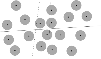
Figure 1: A set of $18$ disks in $\mathds{R}^{2}$ and three separators. The dashed line forms a 6-separator. Both the solid line and the dotted line are halving lines. The solid line is preferable to the other two lines because it separates perfectly and intersects no disks.

1 Introduction

Let $\mathcal{D}$ be a set of $n$ pairwise disjoint unit balls in $\mathds{R}^{d}$ and $P$ the set of their center points. A hyperplane $\mathcal{H}$ is an $m$-separator for $\mathcal{D}$ if each closed halfspace bounded by $\mathcal{H}$ contains at least $m$ points from $P$. This generalizes the notion of halving hyperplanes, which correspond to $n/2$-separators. The analogous notion of separating hyperplanes for point sets has been well studied (see, e.g, [11] for a survey). Separators have various applications, for instance in divide-and-conquer schemes (we discuss some explicit examples below). In such a scheme any ball that is intersected by the separating hyperplane may still interact with both sides of the partition. Therefore it is desirable that the separating hyperplane intersects a small number of balls only.

Alon, Katchalski and Pulleyblank [1] prove that for any set $\mathcal{D}$ in $\mathds{R}^{2}$, there exists a direction such that every line with this direction intersects $O(\sqrt{n\log n})$ disks. In particular, this guarantees the existence of a halving line that intersects at most $O(\sqrt{n\log n})$ disks. Löffler and Mulzer [10] observed that this proof gives a randomized linear-time algorithm. In this paper, we present the following three deterministic algorithms, each of which computes an $m$-separator that intersects $O(n)$ balls for various $m$.

Theorem 1.

Given a set $\mathcal{D}$ of $n$ pairwise disjoint unit balls in $\mathds{R}^{d}$ and $\alpha\in(0,1/2)$, one can construct in $O((1-2\alpha)n)$ time a hyperplane $\mathcal{H}$ that intersects $O((n/(1-2\alpha))^{(d-1)/d})$ balls from $\mathcal{D}$ and such that each closed halfspace bounded by $\mathcal{H}$ contains at least $\alpha n$ centers of balls from $\mathcal{D}$. The constants hidden by the asymptotic notation depend on $d$ only.

Theorem 2.

Given a set $\mathcal{D}$ of $n$ pairwise disjoint unit balls in $\mathds{R}^{d}$ and a function $f(n)\in\omega(1)\cap O(\log n)$, one can construct in $O(nf(n))$ time a hyperplane $\mathcal{H}$ such that each closed halfspace bounded by $\mathcal{H}$ contains at least $\frac{n}{2}(1-1/f(n))=\frac{n}{2}(1-o(1))$ balls from $\mathcal{D}$.

Theorem 3.

For any set $\mathcal{D}$ of $n$ pairwise disjoint unit disks in $\mathds{R}^{2}$ and any $\varepsilon>0$ one can construct in $O(n)$ time a line $\ell$ that intersects $O(n^{(5/6)+\varepsilon})$ disks from $\mathcal{D}$ and such that each closed halfplane bounded by $\ell$ contains at least $n/2$ centers of disks from $\mathcal{D}$.

We develop a generic algorithm in $\mathds{R}^{d}$ that can be instantiated with different parameters to obtain Theorem 1 and Theorem 2. Note that Theorem 2 improves the separation of the center points (compared to Theorem 1) at the cost of increasing the running time slightly. Theorem 3 computes a true halving line in the plane.

Related work.

Bereg, Dumitrescu and Pach [4] (see also [13, Lemma 9.3.2]) strengthen the initial result of Alon, Katchalski and Pulleyblank slightly by proving that there exists a direction such that any line with this direction has at most $O(\sqrt{n\log n})$ disks within constant distance. They use this lemma to prove that one can always move a set of $n$ unit disks from a start to a target configuration in $3n/2+O(\sqrt{n\log n})$ moves. Their algorithm runs in $O(n^{3/2}{(\log n)}^{-1/2})$ time, which Theorem 3 improves to $O(n\log n)$.

Held and Mitchell [7] introduced a paradigm for modeling data imprecision where the location of a point in the plane is not known exactly. For each point, however, we are given a unit disk that is guaranteed to contain the point. The authors show that after preprocessing the disks in $O(n\log n)$ time, they can construct a triangulation of the actual point set in linear time. Löffler and Mulzer [10] follow the same model to construct the onion layer of an imprecise point set. They observed that the proof by Alon et al. immediately gives a randomized expected linear-time algorithm in the following fashion. Pick an angle $\beta\in[0,\pi]$ uniformly at random and compute a halving line for the disks with slope $\beta$. This halving line intersects at most $O(\sqrt{n\log n})$ unit disks with probability at least $1/2$. Löffler and Mulzer use this algorithm to compute a $(\alpha,\beta)$-space decomposition tree: a data structure similar to a binary space partition in which every line is an $\alpha k$-separator that intersects at most $k^{\beta}$ disks. They show that such a $(1/2+\varepsilon,1/2+\varepsilon)$ space decomposition tree can be computed in $O(n\log n)$ expected time, for every $\varepsilon>0$. Theorem 1 can be used to improve this to $O(n\log n)$ deterministic time. They also present a simple deterministic linear-time algorithm that guarantees that at least $n/10$ of the disks are completely on each side of some axis-parallel line. Next, they describe a more sophisticated, deterministic $O(n\log n)$ algorithm to compute a line $\ell$ such that there are at least $n/2-cn^{5/6}$ disks completely to each side of $\ell$. The algorithm uses an $r$-partition of the plane [12] to find good candidate lines. Theorem 3 can be used to improve running time of this algorithm to $O(n)$.

Tverberg [15] studies a related question. He proves that for every natural number $k$ there is a number $K(k)$, such that given convex pairwise disjoint sets $C_{1},\dots,C_{K(k)}$, there always exists a line with some set completely on one side and $k$ sets completely on the other side. Finally, the question has a continuous counterpart that has been solved recently [6].

Organization.

We develop a generic algorithm to compute a separator in $\mathds{R}^{d}$ (where the trade-off between the number of intersected disks and the number of disk centers on each side is determined by a parameter) and prove Theorem 1 and Theorem 2 in Section 2. We prove Theorem 3 in Section 3. Our algorithm follows the approach used in the linear-time ham-sandwich cut algorithm [9]. It divides the line arrangement dual to the set of disk center points by vertical lines such that each slab (the region bounded by two consecutive vertical lines) contains at most a constant fraction of the vertices of the arrangement. In each iteration, the algorithm chooses a slab and discards the rest of the arrangement.

2 Separating balls in $\mathds{R}^{d}$

In this section, we develop a generic algorithm to compute a separator for a given set of pairwise disjoint unit balls in $\mathds{R}^{d}$. Using this generic algorithm, we will give two algorithms to compute an approximately halving hyperplane that intersects a sublinear number of balls.

Besides the set $\mathcal{D}$ of $n$ balls in $\mathds{R}^{d}$, the generic algorithm has two more parameters. First, a number $b\in\{1,\ldots,n\}$ that quantifies the quality of the approximation: we will show that the hyperplane constructed by the algorithm forms an $(n-b)/2$-separator for $\mathcal{D}$. The main step of the algorithm consists in finding a direction $d$ such that we are guaranteed to find a desired separator that is orthogonal to $d$. A second parameter $k\in\mathds{N}$ of the algorithm specifies the number of different directions to generate and test during this step. As a rule of thumb, generating more directions results in a better solution, but the runtime of the algorithm increases proportionally. The algorithm works for certain combinations of these parameters only, as detailed in the following theorem.

Theorem 4.

Given a set $\mathcal{D}$ of $n$ pairwise disjoint unit balls in $\mathds{R}^{d}$ and parameters $b\in\{1,\ldots,n\}$ and $k\in\mathds{N}$ that satisfy the conditions

$$dn \leq kb\quad\mathrm{and}$$ (5)

$$t:=\left({\frac{V_{d}}{2d^{(d-2)/2}}}\right)^{1/d}\frac{n^{1/d}}{k^{2-1/d}} > 2,$$ (6)

(where $V_{d}$ is the volume of the $d$-dimensional unit ball), one can construct in $O(kn)$ time a hyperplane $\mathcal{H}$ that intersects at most $2b/(t-2)$ balls from $\mathcal{D}$ and such that each closed halfspace bounded by $\mathcal{H}$ contains at least $(n-b)/2$ centers of balls from $\mathcal{D}$.

Perhaps more interesting than Theorem 4 in its full generality are the special cases stated as Theorem 1 and Theorem 2 above. Theorem 1 describes the case that $k$ is constant. It can be obtained by choosing $b=\lfloor(1-2\alpha)n\rfloor$ and $k=\lceil(1-2\alpha)d\rceil$ for $\alpha\in(0,1/2)$. Theorem 2 describes the case that $k$ is a very slowly growing function $f(n)$. It can be obtained by choosing $b=n/f(n)$ and $k=df(n)$.

Overview of the algorithm.

Our algorithm consists of two steps. In the first step, we find a direction $d$ in which the balls from $\mathcal{D}$ are “spread out nicely”. More precisely, for an arbitrary (oriented) line $\ell$ consider the set $P$ of points that results from orthogonally projecting all centers of balls from $\mathcal{D}$ onto $\ell$. Denote by $p_{1},\ldots,p_{n}$ the order of points from $P$ sorted along $\ell$. We want to find an $(n-b)/2$-separator orthogonal to $\ell$. This means that the separating hyperplane $\mathcal{H}$ must intersect $\ell$ somewhere in between $p_{(n-b)/2}$ and $p_{(n+b)/2}$.

However, we also need to guarantee that not too many points from $P$ are within distance one of $\mathcal{H}$, which may or may not be possible depending on the choice of $\ell$. Therefore we try several possible directions/lines and select the first one among them that works. In order to evaluate the quality of a line, we use as a simple criterion the spread, defined to be the distance between $p_{(n-b)/2}$ and $p_{(n+b)/2}$. Given a line $\ell$ with sufficient spread, we can find a suitable $(n-b)/2$-separator orthogonal to $\ell$ in the second step of our algorithm, as the following lemma demonstrates. Note the safety cushion of width one to the remaining disks of $\mathcal{D}$.

Lemma 7.

Given a set $P$ of $b$ (one-dimensional) points in an interval $[\ell,r]$ of length $w=r-\ell>2$, we can find in $O(b)$ time a point $p\in(\ell+1,r-1)$ such that at most $2b/(w-2)$ points from $P$ are within distance one of $p$.

Proof.

We select $\lceil(w-2)/2\rceil$ pairwise disjoint closed sub-intervals of length two in $(\ell,r)$. By the pigeonhole principle at least one these intervals contains at most $b/\lceil(w-2)/2\rceil\leq 2b/(w-2)$ points from $P$. Select $p$ to be the midpoint of such an interval.

Algorithmically, we can find such an interval using a kind of binary search on the intervals: We maintain a set of points and a range of intervals. At each step consider the median interval $I$ and test for every point whether it lies in $I$, to the left of $I$, or to the right of $I$. Then either $I$ contains at most $2b/(w-2)$ points from $P$ and we are done, or we recurse on the side that contains fewer points, after discarding all points and intervals on the other side. The process stops as soon as the current range of intervals contains at most $2b/(w-2)$ points from $P$, at which point any of the remaining intervals can be chosen. Given that we maintain the ratio between the number of points and the number of intervals, the process terminates with an interval of the desired type. As the number of points decreases by a constant factor in each iteration, the overall number of comparisons can be bounded by a geometric series and the resulting runtime is linear. ∎

How to find a good direction.

Our algorithm tries $k$ different directions and stops as soon as it finds a direction with spread at least $t$ (see Theorem 4). For a given direction the spread can be computed in $O(n)$ time using linear time rank selection [5]. In the remainder of this section, we will discuss how to select an appropriate set of directions such that one direction is guaranteed to have spread at least $t$.

For this we need a bound on the number of balls simultaneously within distance $w_{1},\ldots,w_{d}$ of some hyperplanes $\mathcal{H}_{1},\ldots,\mathcal{H}_{d}$. Below we give an easy formula based on a volume argument. This formula in turn motivates our choice of directions, which we will explain thereafter.

Lemma 8.

Let $\vec{v}_{1},\vec{v}_{2},\ldots,\vec{v}_{d}\in S^{d-1}\subset\mathds{R}^{d}$ be linearly independent directions and $\mathcal{H}_{1},\mathcal{H}_{2},\ldots,\mathcal{H}_{d}$ hyperplanes with corresponding normal directions, then the maximal number of pairwise disjoint unit balls entirely within distance $w_{1},\ldots,w_{d}$ of $\mathcal{H}_{1},\mathcal{H}_{2},\ldots,\mathcal{H}_{d}$, respectively, is bounded from above by

$$\frac{2^{d}w_{1}\ldots w_{d}}{|\det\left(\vec{v}_{1},\ldots,\vec{v}_{d}\right)|V_{d}},$$

where $V_{d}$ denotes the volume of the $d$-dimensional unit ball.

Proof.

For each hyperplane $\mathcal{H}_{i}$ consider the region $S_{i}$ within distance $w_{i}$ of $\mathcal{H}_{i}$. We want to count the number of balls in $S:=\bigcap_{i}S_{i}$. As each ball has volume $V_{d}$ and they are pairwise disjoint, it is sufficient to bound the volume of $S$. The volume of $S$ depends linearly on $w_{1},\ldots,w_{d}$, so we scale them all to one. We can map the linearly independent vectors $(\vec{v}_{1},\ldots,\vec{v}_{d})$ to the standard basis $(e_{1},\ldots,e_{d})$ by multiplying with the matrix $(\vec{v}_{1},\ldots,\vec{v}_{d})^{-1}$. The volume changes by this transformation by a factor of $1/\det(\vec{v}_{1},\ldots,\vec{v}_{d})$. After this transformation, $S^{\prime}$ is a cube with side length two. ∎

The bound in Lemma 8 depends on the determinant formed by the $d$ direction vectors, which corresponds to the volume of the $(d-1)$-simplex spanned by them. In order to obtain a good upper bound, we must guarantee that this volume does not become too small. Ensuring this reduces to the Heilbronn Problem: Given $k\in\mathds{N}$ and a compact region $P\subset\mathds{R}^{d}$ of unit volume, how can we select $k$ points from $P$ as to maximize the area of the smallest $d$-simplex formed by these points? Heilbronn posed this question for $d=2$, the natural generalization to higher dimension was studied by Barequet [3] and Lefmann [8]. We use the following simple explicit construction in $\mathds{R}^{2}$ that goes back to Erdős and was generalized to higher dimension by Barequet.

Lemma 9 ([3, 14]).

Given a prime $k$, let $P=\{p_{0},\ldots,p_{k-1}\}\subset{[0,1]}^{d}$ with

$$p_{i}=\frac{1}{k}\left(i,i^{2}\mathop{\mathrm{mod}}k,\ldots,i^{d}\mathop{\mathrm{mod}}k\right).$$

Then the smallest $d$-simplex spanned by $d+1$ points from $P$ has volume at least $1/(d!k^{d})$.

Assuming $k$ to be prime is not a restriction: If $k$ is not prime, then by Bertrand’s postulate there is a prime $k^{\prime}\leq 2k$. We can compute $k^{\prime}$ efficiently, for instance, in $O(k/\log\log k)$ time using Atkin’s sieve [2]. In order to obtain the desired direction vectors we proceed as follows: Use Lemma 9 to generate $k$ points $p_{0},\ldots,p_{k-1}$ in $[0,1]^{d-1}$. Then lift the points to $S^{d-1}\subset\mathds{R}^{d}$ using the map

$$f:(x_{1},\ldots,x_{d-1})\mapsto\frac{(x_{1}-\frac{1}{2},\ldots,x_{d-1}-\frac{1}{2},\frac{1}{2})}{||(x_{1}-\frac{1}{2},\ldots,x_{d-1}-\frac{1}{2},\frac{1}{2})||}$$

and denote the resulting set of directions by $D=\{\vec{v}_{0},\ldots,\vec{v}_{k-1}\}$ with $\vec{v}_{i}=f(p_{i})$.

Lemma 10.

For any $d$ vectors $\vec{v}_{i_{1}},\ldots,\vec{v}_{i_{d}}$ from $D$ we have $|\det(\vec{v}_{i_{1}},\ldots,\vec{v}_{i_{d}})|\geq 2^{d-1}/((d-1)!d^{d/2}k^{d-1})$.

Proof.

Let $p_{j}=(x_{j,1},\ldots,x_{j,d-1})$, for $j\in\{0,\ldots,d\}$. Then

$$|\det(\vec{v}_{i_{1}},\ldots,\vec{v}_{i_{d}})| = \left|\det\left(\begin{array}[]{ccc}x_{i_{1},1}-\frac{1}{2}&\ldots&x_{i_{d},1}-\frac{1}{2}\\ \vdots&\ddots&\vdots\\ x_{i_{1},d-1}-\frac{1}{2}&\ldots&x_{i_{d},d-1}-\frac{1}{2}\\ \frac{1}{2}&\ldots&\frac{1}{2}\end{array}\right)\right|\prod_{j=1}^{d}\frac{1}{||(x_{i_{j},1}-\frac{1}{2},\ldots,x_{i_{j},d-1}-\frac{1}{2},\frac{1}{2})||}$$

$$= \frac{1}{2}\left|\det\left(\begin{array}[]{ccc}x_{i_{1},1}&\ldots&x_{i_{d},1}\\ \vdots&\ddots&\vdots\\ x_{i_{1},d-1}&\ldots&x_{i_{d},d-1}\\ 1&\ldots&1\end{array}\right)\right|\prod_{j=1}^{d}\frac{1}{||(x_{i_{j},1}-\frac{1}{2},\ldots,x_{i_{j},d-1}-\frac{1}{2},\frac{1}{2})||},$$

where the determinant on the previous line describes the volume of the $(d-1)$-simplex spanned by $p_{i_{1}},\ldots,p_{i_{d}}$. According to Lemma 9 this determinant is bounded by $1/((d-1)!k^{d-1})$ from below. Also note that all $p_{i}$ are in the unit cube and so all coordinates of the vector $(x_{i_{j},1}-\frac{1}{2},\ldots,x_{i_{j},d-1}-\frac{1}{2},\frac{1}{2})$ are between $-1/2$ and $1/2$. It follows that

$$|\det(\vec{v}_{i_{1}},\ldots,\vec{v}_{i_{d}})|\geq\frac{1}{2(d-1)!k^{d-1}}\prod_{j=1}^{d}\frac{1}{\sqrt{d/4}}=\frac{2^{d-1}}{(d-1)!d^{d/2}k^{d-1}}.\qed$$

We are now ready to prove Theorem 4.

Proof.

The algorithm goes as follows. Compute directions $\vec{v}_{1},\ldots,\vec{v}_{k}$ as in Lemma 10. For each $i\in\{1,\ldots,k\}$ consider the sequence of center points of the disks in $\mathcal{D}$, sorted according to direction $\vec{v}_{i}$, and denote by $S_{i}$ the middle $b$ points in this order (rank $(n-b)/2$ up to $(n+b)/2$). We can bound

$$kb=\sum_{i=1}^{k}|S_{i}|\leq(d-1)n+\sum_{i_{1}<\ldots<i_{d}}|S_{i_{1}}\cap\ldots\cap S_{i_{d}}|,$$

noting that a point that is contained in at most $d-1$ sets $S_{i}$ is counted $d-1$ times on the right hand side, whereas a point that is contained in $a\geq d$ sets is counted $d-1+\binom{a}{d}\geq a$ times.

Denote by $w_{i}$ the width of $S_{i}$ in direction $\vec{v}_{i}$ (which is the spread of $\vec{v}_{i}$). We claim that $w_{i}\geq t$, for some $i\in\{1,\ldots,k\}$.

For the purpose of contradiction assume $w_{i}<t$, for all $i\in\{1,\ldots,k\}$. Together with Lemma 8 and Lemma 10 we get

$$kb = \sum_{i=1}^{k}|S_{i}|\leq(d-1)n+\sum_{i_{1}<\ldots<i_{d}}\frac{2^{d}w_{i_{1}}\ldots w_{i_{d}}}{|\det\left(\vec{v}_{i_{1}},\ldots,\vec{v}_{i_{d}}\right)|V_{d}}$$

$$< (d-1)n+\sum_{i_{1}<\ldots<i_{d}}\frac{2^{d}t^{d}}{V_{d}}\frac{(d-1)!d^{d/2}k^{d-1}}{2^{d-1}}$$

$$= (d-1)n+\binom{k}{d}\frac{2t^{d}(d-1)!d^{d/2}k^{d-1}}{V_{d}}$$

$$\leq (d-1)n+\frac{2d^{(d-2)/2}}{V_{d}}t^{d}k^{2d-1}.$$

In combination with Condition (5) we get

$$dn\leq kb<(d-1)n+\frac{2d^{(d-2)/2}}{V_{d}}t^{d}k^{2d-1}$$

and so

$$t^{d}>\frac{V_{d}}{2d^{(d-2)/2}}\frac{n}{k^{2d-1}},$$

in contradiction to the definition of $t$ in Condition (6). Therefore, our assumption $w_{i}<t$, for all $i\in\{1,\ldots,k\}$, was wrong and there is some $w_{j}\geq t$.

Using Lemma 7 on the set $S_{j}$ projected to a line in direction $\vec{v}_{j}$ we obtain a hyperplane $\mathcal{H}$ orthogonal to $\vec{v}_{j}$ that intersects at most $2b/(w_{j}-2)\leq 2b/(t-2)$ balls from $\mathcal{D}$. By Lemma 7 the hyperplane $\mathcal{H}$ has distance greater than one to any disk in $\mathcal{D}$ whose center is not in $S_{j}$, and so $\mathcal{H}$ is the desired separator.

Regarding the runtime bound, as stated above we can compute the spread of any direction in $O(n)$ time, which yields $O(kn)$ time for $k$ directions. The second step of finding $\mathcal{H}$ can be done in $O(b)=O(n)$ time by Lemma 7. Therefore the overall runtime is $O(kn)$. ∎

3 A deterministic linear time algorithm in the plane

In this section we describe a deterministic linear time algorithm to construct a halving line $\ell$ for a given set $\mathcal{D}$ of $n$ disks in the plane. The line $\ell$ bisects $\mathcal{D}$ perfectly (at most $n/2$ centers lie on either side) and it intersects at most $O(n^{c})$ disks, where $c$ may be chosen arbitrarily close to $5/6$. We may assume that $n$ is odd: If $n$ is even, remove one arbitrary disk and observe that any halving line for the resulting set of disks is also a halving line for the original set. As our algorithm works in the dual arrangement, we first briefly review this duality and how it applies to line-disk intersections.

Point-line duality.

The standard duality transform maps a point $p=(p_{x},p_{y})$ to the line $p^{*}\colon y=p_{x}x-p_{y}$ and a non-vertical line $g:y=mx+b$ to the point $g^{*}=(m,-b)$. This transformation is both incidence preserving ($p\in g\iff g^{*}\in p^{*}$) and order preserving ($p$ is above $g$ $\iff$ $g^{*}$ is above $p^{*}$). Given a set $P$ of points in the plane, the dual arrangement $\mathcal{A}(P^{*})$ is defined by the lines in $P^{*}=\{p^{*}\mid p\in P\}$. In order to avoid parallel lines we assume that no two points in $P$ have the same $x$-coordinate (which can be achieved by an infinitesimal rotation of the plane).

A halving line $\ell$ for $P$ corresponds to a point $\ell^{*}$ in the dual arrangement that has no more than half of the lines from $P^{*}$ above it and no more than half of the lines below it. The set of these points is referred to as the median level of the arrangement induced by $P^{*}$. Since $n$ is odd, for any $x$-coordinate there is exactly one such point, and so we can regard the median level as a function from $\mathds{R}$ to $\mathds{R}$. The following lemma characterizes line-disk intersections in the dual plane.

Lemma 13.

Let $\ell:y=mx+b$ be a non-vertical line and let $p$ denote the center of a unit disk $D$. Then $D$ intersects $\ell$ if and only if the line $p^{*}$ intersects the vertical segment $s=[(m,-b-\sqrt{m^{2}+1}),(m,-b+\sqrt{m^{2}+1})]$.

Proof.

Consider $\ell$ and the two lines $\ell_{a}$ (above) and $\ell_{b}$ (below) at distance $1$ from $\ell$ (Figure 2). Then $D$ intersects $\ell$ if and only if $p$ is below $\ell_{a}$ and above $\ell_{b}$. Equivalently, in the dual, $D$ intersects $\ell$ if and only if $p^{*}$ intersects the vertical line segment $\ell_{a}^{*}\ell_{b}^{*}$ at $x=m$. It remains to calculate the $y$-coordinates of the endpoints of $\ell_{a}^{*}\ell_{b}^{*}$.

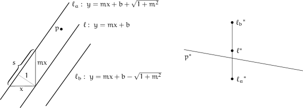
Figure 2: When does a line $\ell$ intersect a unit disk centered at $p$?

Consider a right-angled triangle $T$ for which one side determines the horizontal distance $x$ and another side determines the vertical distance $mx$ between $\ell$ and $\ell_{a}$. Denote the length of the third side of $T$ by $s$. Then the area of $T$ is $\frac{1}{2}s=\frac{1}{2}mx^{2}$. By Pythagoras we have $s^{2}=x^{2}(1+m^{2})$, which together yields $1+m^{2}={(mx)}^{2}$, and so $mx=\sqrt{1+m^{2}}$. ∎

If we view Lemma 13 from the perspective of a unit disk $D$ with center $p$, then the set of lines that intersect $D$ dualizes to the set of points $(x,y)$ whose vertical distance to $p^{*}$ is at most $\sqrt{1+x^{2}}$. We call this closed region of points the (dual) $1$-tube of $D$ (figurename 3). Note that the function $\sqrt{1+x^{2}}$ is strictly convex and so the $1$-tube is bounded by a strictly convex function from above and by a strictly concave function from below.

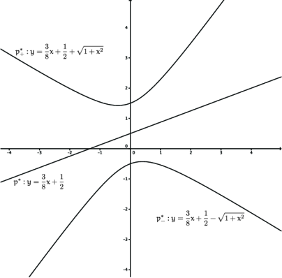
Figure 3: The $1$-tube of the disk centered at $p=(3/8,-1/2)$. It is bounded from below by the function $p^{*}_{-}=p^{*}-\sqrt{1+x^{2}}$ and from above by $p^{*}_{+}=p^{*}+\sqrt{1+x^{2}}$.

Overview of the algorithm.

The algorithm works in the dual arrangement and follows the prune and search paradigm. At the beginning we consider all potential halving lines, but subsequently narrow the range of potential slopes for the desired halving line. Recall that in the dual a halving line appears as a point on the median level, whose x-coordinate corresponds to the slope of the (primal) line.

The successive narrowing of the range of slopes under consideration is made explicit by a parameter $S$, denoting the closed region bounded by at most two vertical lines. Such a region we call a slab. A slab $S=\{(x,y)\in\mathds{R}^{2}\colon\ell\leq x\leq r\}$ we denote by $S={<}\ell,r{>}$. The distance $r-\ell$ between the two bounding vertical lines is the width of $S$. By Alon et al. [1] we may start with $S={<}0,1{>}$ as an initial slab, that is, there is always a halving line that intersects few disks and whose slope is between zero and one.

Crucial for the linear runtime bound is that a constant fraction of all lines from $L$ be discarded after each iteration. However, by discarding some lines also our level of interest—which is the median level of the original set of lines—changes. Therefore this level also appears as a parameter of the algorithm. We denote this parameter by $\lambda\in\{1,2,\ldots,|L|\}$. Initially $\lambda=\lceil n/2\rceil$.

We first describe a single iteration of the algorithm, then prove some bounds for the parameters, and finally present the analysis of the whole algorithm.

A single iteration.

At the beginning of each iteration we have a set $L$ of $n$ lines, a slab $S={<}\ell,r{>}$ of width $w=r-\ell$, and a level parameter $\lambda$. Our goal is to find a constant fraction of lines from $L$ that can be discarded. The outline of an iteration step is as follows.

1. Divide $S$ in constantly many slabs $S_{1},\ldots,S_{m}$, such that each contains at most $\alpha\binom{n}{2}$ many vertices of the arrangement $\mathcal{A}(L)$, for some appropriate constant $0<\alpha<1$. We define $S_{i}={<}\ell_{i},r_{i}{>}$ and $w_{i}=r_{i}-\ell_{i}$.

2. For each slab $S_{i}$, construct a trapezoid $T_{i}\subseteq S_{i}$ such that $T_{i}$ contains the $\lambda$-level of $\mathcal{A}(L)$ within $S_{i}$ and at most half of the lines from $L$ intersect $T_{i}$.

3. For each trapezoid $T_{i}$, define its $1$-tube $\tau_{i}\supset T_{i}$ as follows: Consider the two lines $a_{i}$ and $b_{i}$ passing through the segment bounding $T_{i}$ from above and below, respectively; then $\tau_{i}$ is defined as the closed subset of $S_{i}$ that is bounded by the upper boundary of the $1$-tube of $a_{i}$ from above and by the lower boundary of the $1$-tube of $b_{i}$ from below (Figure 4).

   For each slab $S_{i}$ and some parameter $\gamma\in(0,1/2)$, define the $\gamma$-core $\mathrm{C}_{\gamma}$ of $S_{i}$ to be the central $(1-2\gamma)$-section of $S_{i}$, that is, $\mathrm{C}_{\gamma}(S_{i})={<}\ell_{i}+\gamma w_{i},r_{i}-\gamma w_{i}{>}$.

   For each slab $S_{i}$, count the number $n_{i}$ of lines that intersect $\tau_{i}$ within $\mathrm{C}_{\gamma}(S_{i})$.

4. Select (in a way to be described) one of the slabs $\mathrm{C}_{\gamma}(S_{i})$ to continue the search with. Discard all lines from $L$ that do not intersect $\tau_{i}$ within $\mathrm{C}_{\gamma}(S_{i})$ and adjust $\lambda$ accordingly (decrease by the number of lines discarded that are below $\tau_{i}$).

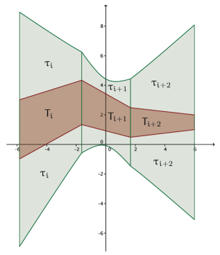
Figure 4: Three consecutive trapezoids $T_{i},T_{i+1},T_{i+2}$ (shown in dark red) and their encompassing $1$-tubes $\tau_{i},\tau_{i+1},\tau_{i+2}$, respectively (shown in light green). In our algorithm, all trapezoids are contained in ${<}0,1{>}$; in this figure they are spread out further so as to emphasize the convex/concave boundary of the $1$-tubes (which would be hard to recognize, otherwise).

Observe first that discarding lines as described in Step 4 is justified: A line $\ell\in L$ that does not intersect $\tau_{i}$ within $\mathrm{C}_{\gamma}(S_{i})$ by Lemma 13 corresponds to a unit disk centered at $\ell^{*}$ that within $\mathrm{C}_{\gamma}(S_{i})$ is not intersected by any line whose dual point lies on the $\lambda$-level of $\mathcal{A}(L)$.

Next we will detail the steps listed above and analyze their runtime. For the first two steps we apply the machinery due to Lo et al. [9]. The first step can be handled in linear time using the following lemma, which follows from Lemma 3.3 of Lo et al. with $\alpha=1/32$.

Lemma 14 ([9]).

Let $L$ be a set of $n$ lines in the plane in general position and let $S$ be a slab. In $O(n)$ time $S$ can be subdivided into subslabs $S_{1},S_{2},\ldots,S_{m}\subset S$ (for some constant $m\leq 64$), such that each $S_{i}$ contains at most $\frac{1}{32}\binom{n}{2}$ of the $\binom{n}{2}$ vertices of $\mathcal{A}(L)$.

The trapezoids mentioned in the second step can be computed as follows. For $S_{i}={<}\ell_{i},r_{i}{>}$, let the upper left (right) corner of $T_{i}$ be defined by the $(\lambda+n/8)$-level of $\mathcal{A}(L)$ at $x=\ell_{i}$ ($x=r_{i}$). Analogously, the lower corners of $T_{i}$ are defined by the $(\lambda-n/8)$-level of $\mathcal{A}(L)$ at $x=\ell_{i}$ ($x=r_{i}$). Then Lemma 3.5 from the paper by Lo et al. (with $\delta=1/8$) gives the following:

Lemma 15 ([9]).

The trapezoid $T_{i}$ contains the $\lambda$-level of $\mathcal{A}(L)$ within $S_{i}$ and at most half of the lines from $L$ intersect $T_{i}$.

All these trapezoids can be constructed in a brute-force manner in $O(n)$ time (recall that $m$ is constant). This completes the first two steps: we have computed (in linear time) a subdivision of our initial slab $S$ into $m\leq 64$ subslabs $S_{i}$, each of which contains a trapezoid $T_{i}$ that contains the $\lambda$-level of $\mathcal{A}(L)$ within $S_{i}$ and at most half of the lines from $L$ intersect $T_{i}$.

Regarding Step 3, note that testing whether a given line intersects $\tau_{i}$ is a geometric predicate of constant algebraic degree and, therefore, can be done in constant time. Hence this step can be executed in a straightforward manner in $O(mn)=O(n)$ time. It remains to argue how to select an appropriate slab to continue with in Step 4. It turns out that not only the number of lines matters, but it is also important to ensure that the width of the slab does not become too small. The following lemma gives a precise account for the bounds we are after.

Lemma 16.

For any $0<\varepsilon<1/2$ and $0<\gamma<1/2$ there exist an integer $n^{\prime}>0$ and constants $m\leq 64$ and $c={(8m/\gamma\varepsilon)}^{2}$ such that for any $n\geq n^{\prime}$ the following statement holds.

Given a set $L$ of $n$ lines, an integer $\lambda\in\{1,\ldots,n\}$, and a slab $S\subseteq{<}0,1{>}$ of width $w\geq c\log(n)/n$, there exist a set $L^{\prime}\subset L$ of at most $(\frac{1}{2}+\varepsilon)n$ lines and a slab $S^{\prime}$ of width $\geq(1-2\gamma)w/m$ such that inside $S^{\prime}$ the $\lambda$-level of $\mathcal{A}(L)$ does not intersect any line in $L\setminus L^{\prime}$.

Analysis of the algorithm.

Let us postpone the proof of Lemma 16 for now and first complete the overall analysis of the algorithm. Denote by $n_{t}$ the number of lines and by $w_{t}$ the width of the current slab after $t$ iterations. We have $n_{0}=n$ and $w_{0}=1$. By Lemma 16 we have

$$n_{t}\leq\left(\frac{1}{2}+\varepsilon\right)^{t}n\quad\mbox{and}\quad w_{t}\geq\left(\frac{1-2\gamma}{m}\right)^{t},$$

as long as $w\geq c\log(n)/n$. After some number of iterations, either we are left with a constant number of lines or a slab of width $w<c\log(n)/n$. As in the first case we can finish by brute force, let us concentrate on the second case. Suppose $t^{*}$ is the smallest index for which $w_{t^{*}}<c\log(n)/n$. The following inequalities are equivalent:

$$\left(\frac{1-2\gamma}{m}\right)^{t^{*}} < \left(\frac{8m}{\gamma\varepsilon}\right)^{2}\cdot\frac{\log n}{n}$$

$$-t^{*}\log\left(\frac{m}{1-2\gamma}\right) < 2\log\left(\frac{8m}{\gamma\varepsilon}\right)+\log\log n-\log n$$

$$t^{*} > \frac{\log n-2\log\left(\frac{8m}{\gamma\varepsilon}\right)-\log\log n}{\log\left(\frac{m}{1-2\gamma}\right)}.$$

Since $\gamma$, $\varepsilon$ and $m$ are all constant, the last inequality implies that for any constant $0<\varepsilon^{\prime}<1$ we have

$$t^{*}>\log n\cdot\frac{(1-\varepsilon^{\prime})}{\log(\frac{m}{1-2\gamma})}\,,$$

for sufficiently large $n$ (depending on $\varepsilon^{\prime}$). Hence the number of lines to be considered after $t^{*}$ iterations is

$$n_{t^{*}} \leq \left(\frac{1}{2}+\varepsilon\right)^{t^{*}}\cdot n$$

$$< \left(\frac{1}{2}+\varepsilon\right)^{\log n\frac{1-\varepsilon^{\prime}}{\log(\frac{m}{1-2\gamma})}}\cdot n$$

$$= n^{\log\left(\frac{1}{2}+\varepsilon\right)\frac{1-\varepsilon^{\prime}}{\log(\frac{m}{1-2\gamma})}}\cdot n$$

$$= n^{\log\left(\frac{1}{2}+\varepsilon\right)\frac{1-\varepsilon^{\prime}}{\log(\frac{m}{1-2\gamma})}+1}$$

$$\leq n^{\frac{5}{6}+\delta}$$

where the last inequality uses $m\leq 64$ (and hence $\log m\leq 6$) and where $\delta>0$ can be made arbitrarily small by choosing $\varepsilon$, $\varepsilon^{\prime}$ and $\gamma$ to be correspondingly small.

So after at most $t^{*}=\Theta(\log n)$ iterations we are left with a slab $S$ and $O(n^{\frac{5}{6}+\delta})$ lines. All lines that have been discarded do not intersect the $1$-tube of the level that corresponds to the original median level. Therefore any point on this level within $S$ corresponds to a halving line for the original set of disks that intersects $o(n)$ of the disks. Such a point can easily be found in a brute force manner in $o(n)$ time.

Denote by $R(n)$ the runtime of the algorithm for $n$ disks. Each iteration can be handled in time linear in the number of lines/disks remaining and so

$$R(n)\leq\sum_{t=0}^{t^{*}}cn_{t}\leq cn\sum_{t=0}^{t^{*}}\left(\frac{1}{2}+\varepsilon\right)^{t}<\frac{2c}{1-2\varepsilon}n=O(n),$$

for some constant $c$. This proves Theorem 3.

Proof of Lemma 16.

It remains to prove that we can select a constant fraction of lines to be discarded in each iteration while at the same time the width of the current slab does not shrink too much. To begin with we need a slab whose $1$-tube is not intersected by too many lines. To show that such a slab exists, we use an averaging argument: While a single $1$-tube $\tau_{i}$ may be intersected by all lines from $L$, on average the number of intersecting lines per slab is sublinear. To this end we define a function $g$ by setting $g(x)$ to be the number of lines that intersect $\bigcup_{i=1}^{m}\tau_{i}$ at $x\in(\ell,r)$. The following lemma provides an upper bound on the average number of such lines.

Lemma 17.

For a slab $S={<}\ell,r{>}\subseteq{<}0,1{>}$ of width $w=r-\ell$, there is some constant $c\leq 4$ such that

$$\int_{\ell}^{r}g(x)\,\mathrm{d}x\leq c\sqrt{nw\log(nw)}\,,$$

if $nw$ is sufficiently large.

Proof.

We follow the approach of Alon et al. [1] but are more specific about some technical details. We define $x_{i}:=\ell+iw/k$, for $i=0,\ldots,k-1$ and some parameter $k$ to be specified later and consider the function

$$f(x):=\sum_{i=0}^{k-1}g(x+x_{i})$$

over the domain $[0,w/k]$. Clearly, we have

$$\int_{0}^{w/k}f(x)\,\mathrm{d}x=\int_{\ell}^{r}g(x)\,\mathrm{d}x\,.$$

Next we bound $f(x)$ for some arbitrary but fixed $x$. To this end, we move back to the primal setting and consider the set $H$ of halving lines $h_{i}$ with slope $x_{i}+x$, for $i\in\{0,\ldots,k-1\}$. Let $D_{i}$ denote the set of disks from $\mathcal{D}$ that intersect $h_{i}$. The value of $f$ is the number of pairs $(d,h)\in D\times H$ where $d\cap h\neq\emptyset$. A (generous) upper bound for this quantity is provided by

$$n+\sum_{i<j}|D_{i}\cap D_{j}|\,,$$

where the first term counts every disk that intersects only one line and the second term counts every disk that is intersected by at least two lines. (In this way, a disk that is intersected by $c$ lines is counted $1+\binom{c}{2}$ times.)

Let $\vec{v}_{i}={(-x_{i}-x,1)}^{T}/\sqrt{{(x_{i}+x)}^{2}+1}$ be the (unit) normal vector to $h_{i}$. By Lemma 8 (where $d=2$, $w_{1}=w_{2}=2$, $\vec{v}_{1}=\vec{v}_{i}$, and $\vec{v}_{2}=\vec{v}_{j}$) we have (using $x+x_{i}\leq 1$)

$$|D_{i}\cap D_{j}|\leq\frac{16}{\pi\,|\det(\vec{v}_{1},\vec{v}_{2})|}=\frac{16\sqrt{(x_{i}+x)^{2}+1}\sqrt{(x_{j}+x)^{2}+1}}{\pi\,|x_{i}-x_{j}|}\leq\frac{32}{\pi\,|x_{i}-x_{j}|}=\frac{32k}{\pi w\,|i-j|}$$

and therefore

$$n+\sum_{i<j}|D_{i}\cap D_{j}|\leq n+\frac{32k}{\pi w}\sum_{i<j}\frac{1}{j-i}\,.$$

The sum can be bounded using

$$\sum_{i<j}\frac{1}{j-i}=\sum_{a=1}^{k-1}\frac{k-a}{a}=kH_{k-1}-(k-1)<1+k\ln(k)\,,$$

where the last inequality uses the well-known bound $H_{n}<1+\ln(n)$ for the harmonic number. We started out by fixing a particular $x$, but the derived bound holds for any arbitrary $x$. Altogether we obtain

$$f(x)<n+\frac{32k}{\pi w}(1+k\ln(k))=n+\frac{32}{\pi w}(k+k^{2}\ln(k))$$

and so

$$\int_{\ell}^{r}g(x)\,\mathrm{d}x=\int_{0}^{w/k}f(x)\,\mathrm{d}x<\frac{nw}{k}+\frac{32}{\pi}(1+k\ln(k))\,.$$

Setting $k=\left\lceil\sqrt{\pi nw/(16\ln(nw))}\right\rceil$ in the previous expression and omitting the ceilings (it can be verified that this only increases the value of the expression, provided $nw\geq 512$) yields

$$\int_{\ell}^{r}g(x)\,\mathrm{d}x<\frac{4}{\sqrt{\pi}}\sqrt{nw\ln(nw)}+\frac{32}{\pi}+\frac{8}{\sqrt{\pi}}\sqrt{\frac{nw}{\ln(nw)}}\ln\left(\sqrt{\frac{\pi nw}{16\ln(nw)}}\right)\,,$$

which—noting that $\sqrt{\pi x/(16\ln x)}<\sqrt{x}$, for $x\geq 1$—is upper bounded by

$$\frac{4}{\sqrt{\pi}}\sqrt{nw\ln(nw)}+\frac{32}{\pi}+\frac{8}{\sqrt{\pi}}\sqrt{\frac{nw}{\ln(nw)}}\ln(\sqrt{nw})=\frac{8}{\sqrt{\pi}}\sqrt{nw\ln(nw)}+\frac{32}{\pi}.$$

It can be checked that the last expression is upper bounded by $4\sqrt{nw\log_{2}(nw)}$, for $nw\geq 226$. ∎

By the pigeonhole principle, the integral is small for most subslabs. But bounding the integral is not sufficient to bound the number of lines that intersect the $1$-tube, because lines that do so for a very short interval only do not contribute much to the integral. To account for such lines we restrict our focus to the $\gamma$-core of the slabs instead. For a slab $S_{i}$ let $d_{i}(x)$ denote the number of lines that intersect $\tau_{i}\setminus T_{i}$ at $x$, for $x\in(\ell_{i},r_{i})$. Clearly $d_{i}\leq g$. Furthermore let

$$\phi_{\gamma,i}=\max\,\{d_{i}(x)\colon x\times\mathds{R}\subset\mathrm{C}_{\gamma}(S_{i})\}.$$

Proposition 18.

The number of lines from $L$ that intersect $(\tau_{i}\setminus T_{i})\cap\mathrm{C}_{\gamma}(S_{i})$ is bounded by $2\phi_{\gamma,i}$, for any $i\in\{1,\ldots,m\}$ and $0<\gamma<1/2$.

Proof.

Let $\mathrm{C}_{\gamma}(S_{i})={<}a_{i},b_{i}{>}$ and consider a line $\ell$ that intersects $(\tau_{i}\setminus T_{i})\cap\mathrm{C}_{\gamma}(S_{i})$. Then $\ell$ intersects at most one boundary of $\tau_{i}$, say, the upper boundary $U$. As $U$ is strictly convex, the line $\ell$ intersects $\tau_{i}$ at $x=a_{i}$ or $x=b_{i}$ (possibly both). Therefore, the number of such lines is upper bounded by $d_{i}(a_{i})+d_{i}(b_{i})\leq 2\phi_{\gamma,i}$. ∎

Proposition 19.

$\phi_{\gamma,i}w_{i}\leq\gamma^{-1}\int_{\ell_{i}}^{r_{i}}g(x)\,\mathrm{d}x$

Proof.

Let $\mathrm{C}_{\gamma}(S_{i})={<}a_{i},b_{i}{>}$ and consider a line $\ell$ that is counted in $\phi_{\gamma,i}$, that is, $\ell$ intersects $\tau_{i}\setminus T_{i}$ at some $x\in[a_{i},b_{i}]$. By the proof of Proposition 18, we may assume that $x\in\{a_{i},b_{i}\}$. Using the same argumentation, we may also assume that $\ell$ intersects $\tau_{i}$ at some $x^{\prime}\in\{\ell_{i},r_{i}\}$. Regardless of the combination of $x$ and $x^{\prime}$, it follows that $\ell$ contributes to $d_{i}$—and thus to $g$—for at least a $\gamma$-fraction of the interval $[\ell_{i},r_{i}]$. ∎

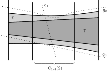
Figure 5: A slab $S$ with its core $\mathrm{C}_{1/4}(S)$ and a corresponding trapezoid $T$ with its $1$-tube $\tau$. The line $g_{1}$ intersects both $T$ and $\tau$, whereas $g_{2}$ and $g_{3}$ intersect $\tau$ but not $T$. Every such line intersects $\tau$ at the boundary of the core, like $g_{3}$ does. An intersection pattern as depicted for $g_{2}$ is impossible for a straight line.

Now we have all tools in place to complete the proof of Lemma 16. Combining Proposition 19 and Lemma 17 yields

$$\sum_{i=1}^{m}\phi_{\gamma,i}w_{i}\leq 4\gamma^{-1}\sqrt{nw\log(nw)}\,.$$

We claim that we can select any slab $S_{j}$ for which $w_{j}\geq w/m$ and continue the search within $\mathrm{C}_{\gamma}(S_{j})$. Such a slab exists because there are $m$ slabs in total and $w=\sum_{i=1}^{m}w_{i}$. We can then bound

$$\phi_{\gamma,j}\frac{w}{m}\leq\phi_{\gamma,j}w_{j}\leq\sum_{i=1}^{m}\phi_{\gamma,i}w_{i}\leq 4\gamma^{-1}\sqrt{nw\log(nw)}$$

and so

$$\phi_{\gamma,j}\leq 4\gamma^{-1}m\,\sqrt{\frac{n\log(nw)}{w}}\leq 4\gamma^{-1}m\,\sqrt{\frac{n\log(n)}{w}}\,.$$

The slab we continue to search in (the core $\mathrm{C}_{\gamma}(S_{j})$ of $S_{j}$) has width at least $(1-2\gamma)w/m$. Lemma 15 and Proposition 18 bound the number $n_{\gamma,j}$ of lines that intersect $\tau_{j}$ within $\mathrm{C}_{\gamma}(S_{j})$ by

$$n_{\gamma,j}\leq\frac{n}{2}+2\phi_{\gamma,j}\leq\frac{n}{2}+\frac{8m}{\gamma}\,\sqrt{\frac{n\log(n)}{w}}\,.$$

Given any $0<\varepsilon<1/2$ and $0<\gamma<1/2$, we have $n_{\gamma,j}\leq\left(\frac{1}{2}+\varepsilon\right)n\,,$ as long as $w\geq\left(\frac{8m}{\gamma\varepsilon}\right)^{2}\cdot\frac{\log n}{n}\,,$ which is stated as an assumption. This completes the proof of Lemma 16.

4 Conclusions

In this paper we studied the construction of separators for balls in deterministic linear time. The aim is to intersect as few balls as possible while (approximately) bisecting the set of center points. We presented essentially two ways to compute such seperators with a sublinear number of intersections. The first algorithm is very simple and straight-forward to implement (we gave all constants explicitly), and obtains an arbitrarily good bisection in combination with an asymptotically optimal number of intersections. The strength of the second algorithm is to bisect the center points exactly, but it works in the plane only.

Throughout the paper we assumed the balls to be disjoint, but we never really used it. In fact, both algorithms work as long as we have some density lower bound on the objects under consideration and some bound on the size of the objects. This lower bound is implicitly given if for instance the objects satisfy some fatness condition and are disjoint. Also note that, in contrast to the continuous case, we do not make use of the fact that the hyperplane to be constructed is bisecting. Therefore it is easy to adapt the algorithm to, for instance, have $n/3$ of the points on one side and $2n/3$ of the other side of the hyperplane.

There are point sets for which the number of balls intersected by every halving hyperplane is $\Omega(n^{(d-1)/d})$. But already for dimension three it is not clear if a halving plane with $o(n^{3/4})$ intersections always exists ($O(n^{3/4})$ is not difficult). In dimension two it is open if $o(\sqrt{n\log n})$ can be achieved. So let us ask the following question: Is it true that for every set of $n$ disjoint unit balls in $\mathds{R}^{d}$ there exists a halving hyperplane that intersects $O(n^{(d-1)/d})$ of the balls?

Acknowledgments.

We want to thank Marek Elias, Jiřka Matoušek, Edgardo Roldán-Pensado and Zuzana Safernová for interesting discussions on the conjecture for higher dimensions and referring us to related work.

References

- [1] Noga Alon, Meir Katchalski, and William R. Pulleyblank, Cutting disjoint disks by straight lines. Discrete & Computational Geometry, 4, (1989), 239–243, URL http://dx.doi.org/10.1007/BF02187724.
- [2] A. Oliver L. Atkin and Daniel J. Bernstein, Prime sieves using binary quadratic forms. Math. Comput., 73, 246, (2004), 1023–1030, URL http://dx.doi.org/10.1090/S0025-5718-03-01501-1.
- [3] Gill Barequet, A lower bound for Heilbronn’s triangle problem in d dimensions. SIAM Journal on Discrete Mathematics, 14, 2, (2001), 230–236, URL http://dx.doi.org/10.1137/S0895480100365859.
- [4] Sergey Bereg, Adrian Dumitrescu, and János Pach, Sliding disks in the plane. International Journal of Computational Geometry & Applications, 18, 05, (2008), 373–387, URL http://dx.doi.org/10.1142/S0218195908002684.
- [5] Manuel Blum, Robert W. Floyd, Vaughan Pratt, Ronald L. Rivest, and Robert E. Tarjan, Time bounds for selection. Journal of Computer and System Sciences, 7, 4, (1973), 448–461, URL http://dx.doi.org/10.1016/S0022-0000(73)80033-9.
- [6] Luca Esposito, Vincenzo Ferone, Bernd Kawohl, Carlo Nitsch, and Cristina Trombetti, The longest shortest fence and sharp Poincaré–Sobolev inequalities. Archive for Rational Mechanics and Analysis, 206, 3, (2012), 821–851, URL http://dx.doi.org/10.1007/s00205-012-0545-0.
- [7] Martin Held and Joseph SB Mitchell, Triangulating input-constrained planar point sets. Information Processing Letters, 109, 1, (2008), 54–56, URL http://dx.doi.org/10.1016/j.ipl.2008.09.016.
- [8] Hanno Lefmann, On Heilbronn’s problem in higher dimension. Combinatorica, 23, 4, (2003), 669–680, URL http://dx.doi.org/10.1007/s00493-003-0040-1.
- [9] Chi-Yuan Lo, Jiří Matoušek, and William L. Steiger, Algorithms for ham-sandwich cuts. Discrete & Computational Geometry, 11, (1994), 433–452, URL http://dx.doi.org/10.1007/BF02574017.
- [10] Maarten Löffler and Wolfgang Mulzer, Unions of onions. CoRR, abs/1302.5328, URL http://arxiv.org/abs/1302.5328.
- [11] Horst Martini and Anita Schöbel, Median hyperplanes in normed spaces – a survey. Discrete Applied Mathematics, 89, 1, (1998), 181–195, URL http://dx.doi.org/10.1016/S0166-218X(98)00103-6.
- [12] Jiří Matoušek, Efficient partition trees. Discrete & Computational Geometry, 8, 1, (1992), 315–334, URL http://dx.doi.org/10.1007/BF02293051.
- [13] János Pach and Micha Sharir, Combinatorial geometry and its algorithmic applications: The Alcalá lectures, vol. 152 of Mathematical Surveys and Monographs. Amer. Math. Soc., 2009.
- [14] Klaus F. Roth, On a problem of Heilbronn. J. London Math. Soc., 26, 3, (1951), 198–204, URL http://dx.doi.org/10.1112/jlms/s1-26.3.198.
- [15] Helge Tverberg, A seperation property of plane convex sets. Mathematica Scandinavica, 45, (1979), 255–260, URL http://eudml.org/doc/166678.