[1405.1875] 1 Time series statistics

ANALYSIS OF SOURCE MOTIONS DERIVED FROM POSITION TIME SERIES

Z. MALKIN, E. POPOVA
              Pulkovo Observatory
              Pulkovskoe Ch., 65, St. Petersburg 196140, Russia
              e-mail: malkin@gao.spb.ru

ABSTRACT. In this paper an attempt is made to extract a systematic part from the source motions obtained from the position time series provided by several IVS Analysis Centers in the framework of the ICRF-2 project. Our preliminary results show that the radio source velocities and the parameters of the systematic part of the velocity field differ substantially between the source position time series, which does not allow us to get a reliable solution for the coefficients of spherical harmonics.

1. INTRODUCTION

Many radio sources observed during astrometric/geodetic VLBI sessions show progressive variations in its position derived from single session solutions. Several physical effects can cause systematic apparent movement of celestial objects. Hence investigation of the radio source apparent velocity field can help in investigations in various fields, such as fundamental physics, cosmology, etc. Several analysis strategies for computation of systematic part in the radio source velocities can be used:

a)

estimate source position and velocities from global solution, then fit spherical harmonics to the velocities (Gwinn et al. 1997);
b)

compute the coefficients of spherical harmonics as global parameters (MacMillan 2005; Titov 2008a, 2008b);
c)

compute velocities from position time series, then fit spherical harmonics to the velocities.

In this paper, we will test the latter approach which, hopefully, can provide a possibility for supplement comparisons and accuracy assessment.

2. DATA USED

For this work we have used 26 source position time series computed at 9 VLBI analysis centers making use of 6 different software, which provides a good opportunity for comparisons.

Table 1 presents data statistics. In the “All sessions” columns, all submitted data are used having at least two sessions (epochs) for the source, which allows us formally to compute the velocity, even not of large scientific meaning.

For more rigorous comparison we also selected the data at common epochs for 17 series. The common epochs were identified by the session name. At this stage we did not use bkg000c series which seems to be just extension of bkg000b with the same positions for the same sessions, gsf000b series which seems to be only preliminary one, aus series which does not contain session ID, and several series with relatively small number of sources. Statistics for thus selected data is shown in Table 1 in the “Common sessions” columns.

Table 1: Time series statistics

Series	Software	All sessions		Common sessions
		Time span	Nsou	Time span	Nsou
aus000a	OCCAM-LSC	1979–2007	75	—	—
aus001a	OCCAM-LSC	1979–2007	578	—	—
aus002a	OCCAM-LSC	1979–2007	470	—	—
aus003a	OCCAM-LSC	1979–2007	503	—	—
bkg000b	Calc/Solve	1984–2007	615	—	—
bkg000c	Calc/Solve	1984–2007	794	1984–2007	463
dgf000a	OCCAM-LS	1984–2007	425	—	—
dgf000b	OCCAM-LS	1984–2007	624	1984–2007	463
dgf000c	OCCAM-LS	1984–2007	624	1984–2007	463
dgf000d	OCCAM-LS	1984–2007	624	1984–2007	463
dgf000e	OCCAM-LS	1984–2007	624	1984–2007	463
dgf000f	OCCAM-LS	1984–2007	680	1984–2007	463
dgf000g	OCCAM-LS	1984–2007	680	1984–2007	463
gsf000b	Calc/Solve	1979–2005	721	—	—
gsf001a	Calc/Solve	1979–2007	742	1984–2007	463
gsf002a	Calc/Solve	1979–2007	754	1984–2007	463
iaa000b	QUASAR	1979–2007	540	1984–2007	463
iaa000c	QUASAR	1979–2007	569	1984–2007	463
mao000b	SteelBreeze	1980–2007	773	1984–2007	463
opa000a	Calc/Solve	1984–2007	507	—	—
opa000b	Calc/Solve	1984–2007	645	1984–2007	463
opa001a	Calc/Solve	1984–2007	519	—	—
opa002a	Calc/Solve	1984–2007	628	1984–2007	463
sai000b	ARIADNA	1984–2007	640	1984–2007	463
usn000d	Calc/Solve	1979–2007	728	1984–2007	463
usn001a	Calc/Solve	1979–2007	728	1984–2007	463

3. COMPARISON OF VELOCITIES

The source velocities were computed as weighted linear drift of the submitted source positions with weights inversely proportional to the reported variances of source positions. Since some time series contain positions with unlikely small errors (down to 1 $\mu$ as in the iaa series), which leads to problems with computing the velocity as the weighted trend, it was decided to use a minimal error value of 20 $\mu$ as, i.e. all errors less then this value were replaced by 20 $\mu$ as. No series except iaa were substantially affected by this procedure.

Our programs for computation of source velocities and spherical harmonics has several optional parameters for data selection: the first epoch, minimum number of sessions, minimum data span, maximum error in velocity. The results presented in this section were computed for all the data presented in the original series having at least 5 sessions and 3-year time span.

In Table 2, the results of computation of the median error in velocity computed for are presented. This values may be an index of the scatter of position time series. One can see that some time series are much more noisy than others.

Table 2: Median errors in velocities. Unit:

\mu

as/yr

Series	All sessions		Common sessions
	$V_{\alpha}\cos\delta$	$V_{\delta}$	$V_{\alpha}\cos\delta$	$V_{\delta}$
aus000a	7	11	–	–
aus001a	19	28	–	–
aus002a	18	26	–	–
aus003a	18	29	–	–
bkg000c	14	18	17	21
dgf000a	19	25	–	–
dgf000b	15	18	18	21
dgf000c	15	21	19	26
dgf000d	15	19	19	23
dgf000e	15	19	19	22
dgf000f	16	23	19	26
dgf000g	16	19	19	23
gsf001a	13	17	15	19
gsf002a	13	17	17	20
iaa000b	15	22	18	22
iaa000c	16	22	20	23
mao000b	23	31	25	34
opa000a	15	19	–	–
opa000b	16	23	19	28
opa001a	15	18	–	–
opa002a	17	19	16	20
sai000b	25	37	30	45
usn000d	13	18	17	20
usn001a	21	29	25	34

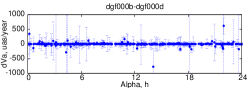
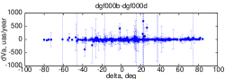
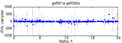
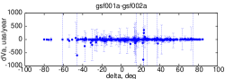
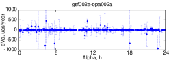
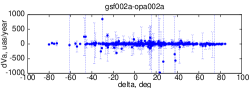
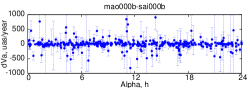
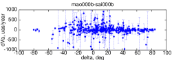
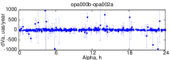
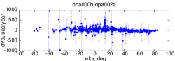
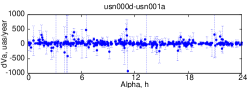
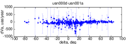
Comparison of velocities obtained from different time series for the same source show sometimes rather large discrepancies. In Fig 1 some examples are given (only data at common epochs were used for rigorous comparison).

Refer to caption — Figure 1: Comparison of source velocities obtained from different time series

4. TEST OF HARMONICS

For test purpose, we compute the coefficients of two spherical harmonics $\Delta H_{12}$ and $\Delta H_{3}$ (Titov 2008a) using the following formulas:

	$\displaystyle\mu_{\alpha}$	$\displaystyle=$	$\displaystyle-\Delta H_{12}\sin 2\alpha\,,$
	$\displaystyle\mu_{\delta}$	$\displaystyle=$	$\displaystyle-\frac{\Delta H_{12}}{4}\cos 2\alpha\sin 2\delta+\frac{\Delta H_{3}}{2}\sin 2\delta.$

We tried several options for data selection which produce different results; however, the difference is usually not so large for reasonable values of the selection criteria given above. In Table 3, the results are presented computed for all the data presented in the original series having at least 5 sessions and 3-year time span. It can be noted that using more strict criteria, such as minimum 10 sessions and 10 years of observations gives statistically similar result, with smaller value of the formal error in the harmonics coefficients when more observations are used. In the last row of the table the results are presented corresponding to the cumulative solution including all the velocity estimates merged all the input time series.

Table 3: Results of computation of

\Delta H_{12}

and

\Delta H_{3}

. Unit:

\mu

Series	All sessions					Common sessions
	Nsou	$\Delta H_{12}$		$\Delta H_{3}$		Nsou	$\Delta H_{12}$		$\Delta H_{3}$
aus000a	71	-8.76 $\pm$	3.15	1.02 $\pm$	2.33	—	—		—
aus001a	343	-4.53 $\pm$	1.08	-2.13 $\pm$	0.87	—	—		—
aus002a	308	-0.34 $\pm$	1.22	-0.47 $\pm$	0.99	—	—		—
aus003a	322	-3.80 $\pm$	1.12	-2.47 $\pm$	0.90	—	—		—
bkg000c	537	-1.01 $\pm$	0.83	0.85 $\pm$	0.74	350	-0.27 $\pm$	0.91	-1.27 $\pm$	0.83
dgf000a	277	-3.84 $\pm$	1.44	4.88 $\pm$	1.49	—	—		—
dgf000b	476	-1.66 $\pm$	0.73	1.12 $\pm$	0.70	350	-1.06 $\pm$	0.74	-0.73 $\pm$	0.71
dgf000c	476	-0.27 $\pm$	0.90	1.23 $\pm$	0.76	350	0.88 $\pm$	0.93	-1.08 $\pm$	0.80
dgf000d	476	-1.94 $\pm$	0.75	1.14 $\pm$	0.72	350	-1.47 $\pm$	0.77	-0.71 $\pm$	0.73
dgf000e	476	-2.08 $\pm$	0.73	1.08 $\pm$	0.71	350	-1.71 $\pm$	0.77	-0.57 $\pm$	0.73
dgf000f	531	-0.29 $\pm$	0.86	1.27 $\pm$	0.71	350	0.85 $\pm$	0.97	-0.88 $\pm$	0.81
dgf000g	531	-2.09 $\pm$	0.71	1.18 $\pm$	0.67	350	-1.83 $\pm$	0.80	-0.43 $\pm$	0.75
gsf001a	582	-0.62 $\pm$	0.70	-0.09 $\pm$	0.64	350	-0.77 $\pm$	0.86	-0.76 $\pm$	0.78
gsf002a	592	-0.39 $\pm$	0.65	0.64 $\pm$	0.59	350	0.50 $\pm$	0.83	-1.46 $\pm$	0.76
iaa000b	458	1.23 $\pm$	1.37	0.80 $\pm$	1.16	350	3.49 $\pm$	1.21	1.70 $\pm$	1.08
iaa000c	481	1.15 $\pm$	1.34	2.16 $\pm$	1.15	350	2.75 $\pm$	1.24	3.44 $\pm$	1.17
mao000b	555	0.05 $\pm$	1.05	1.01 $\pm$	0.86	350	0.14 $\pm$	1.26	-0.35 $\pm$	1.07
opa000a	384	0.11 $\pm$	1.10	-0.46 $\pm$	0.95	—	—		—
opa000b	510	-6.14 $\pm$	1.09	0.46 $\pm$	0.88	350	-10.55 $\pm$	1.52	-1.01 $\pm$	1.21
opa001a	392	0.20 $\pm$	0.99	-0.37 $\pm$	0.87	—	—		—
opa002a	511	0.66 $\pm$	0.87	-0.53 $\pm$	0.77	350	-0.21 $\pm$	0.94	0.15 $\pm$	0.85
sai000b	501	-1.96 $\pm$	1.18	1.79 $\pm$	0.95	350	0.27 $\pm$	1.37	-1.39 $\pm$	1.14
usn000d	572	-0.70 $\pm$	0.78	0.18 $\pm$	0.70	350	-0.25 $\pm$	0.90	-1.44 $\pm$	0.81
usn001a	572	-5.94 $\pm$	1.22	1.53 $\pm$	1.02	350	-6.57 $\pm$	1.67	-0.28 $\pm$	1.38
All data	11477	-1.24 $\pm$	0.19	0.62 $\pm$	0.17	5950	-0.54 $\pm$	0.23	-0.51 $\pm$	0.21

5. CONCLUDING REMARKS

Although most results presented in Table 3 are formally statistically reliable, they differ substantially between input time series, and also between various sets of data selected. This fact, along with results of velocity comparison may indicate that source position time series should be used with care for analysis of the fine effects in the source proper motions.

Further study is needed to investigate a possibility to use combined or cumulative solution as the most reliable estimate of spherical harmonics. In particular, careful selection of input series should be performed. For instance, in our cumulative solution dgf data are clearly overweighted due to 6 series used, often with very similar position estimates. On the other hand, it seems to be inappropriate to use only one series from one analysis center because some centers compute two and more series using quite different approaches, and this would be important to compare all of them, because there is no indisputable proof in favor of only one approach.

6. REFERENCES

Gwinn, C. R., et. al., 1997, ”Quasar proper motions and low-frequency gravitational waves”, ApJ 485, pp. 87-91.

Macmillan, D.S., 2005, “Quasar Apparent Proper Motion Observed by Geodetic VLBI Networks”, In: Future Directions in High Resolution Astronomy: The 10th Anniversary of the VLBA, ASP Conference Proceedings, V. 340. Eds. J. Romney, M. Reid, San Francisco: Astronomical Society of the Pacific, 2005, pp. 477–481.

Titov. O., 2008a, “Proper motions of reference radio sources”, In: Proc. Journées Systèmes de Référence Spatio-temporels 2007, Meudon, France, 17-19 Sep 2007, Ed. N. Capitaine, pp. 16–19.

Titov, O., 2008b, “Systematic effects in proper motion of radio sources”, arXiv:0805.1099.