Guiding ultraslow weak-light bullets with Airy beams in a coherent atomic system

Abstract

We investigate the possibility of guiding stable ultraslow weak-light bullets by using Airy beams in a cold, lifetime-broadened four-level atomic system via electromagnetically induced transparency (EIT). We show that under EIT condition the light bullet with ultraslow propagating velocity and extremely low generation power formed by the balance between diffraction and nonlinearity in the probe field can be not only stabilized but also steered by the assisted field. In particular, when the assisted field is taken to be an Airy beam, the light bullet can be trapped into the main lobe of the Airy beam, propagate ultraslowly in longitudinal direction, accelerate in transverse directions, and move along a parabolic trajectory. We further show that the light bullet can bypass an obstacle when guided by two sequential Airy beams. A technique for generating ultraslow helical weak-light bullets is also proposed.

I Introduction

In the past two decades, much effort has been paid to study of spatial-temporal optical solitons, or light bullets, which describe a fascinating class of nonlinear optical pulses localized in three spatial and one temporal dimensions sil . Due to the balance between diffraction, dispersion, and nonlinearity, these optical pulses are capable of arresting spatial-temporal distortion and propagate stably for a long distance. Light bullets are of great interest because of their rich nonlinear physics and important applications ber ; kiv0 ; mal ; kiv ; liu ; bla ; tow ; tra ; mih ; mat ; ber1 ; bel ; burg ; chen ; abd ; min ; mat1 ; kat1 ; mihalache1 ; mihalache2 ; mihalache3 . However, up to now most light bullets are produced in passive optical media, in which far-off resonance excitation schemes are employed in order to avoid significant optical absorption. For generating the light bullets in passive media, very high light-intensity is usually needed to obtain nonlinearity strong enough to balance the dispersion and diffraction effects. In addition, an active control on the property of light bullets is not easy to realize in passive media because of the absence of energy-level structure and selection rules that can be used and manipulated.

For practical applications, light bullets having low generation power and good controllability are highly desirable. Active optical media, in which light interacts with matter resonantly, can be adopted to achieve such goal. However, in resonant media there is usually a large optical absorption. In order to suppress the large optical absorption, a technique called electromagnetically induced transparency (EIT) har can be used. Due to the quantum interference effect induced by a control field, the propagation of a weak probe field in EIT media exhibits not only large suppression of optical absorption, but also significant reduction of group velocity, and great enhancement of Kerr nonlinearity, etc fle . Based on these important features, new types of temporal wu ; hua ; hang ; yang and spatial hong ; mic ; hang1 ; hang2 optical solitons were predicted in highly resonant atomic systems via EIT. The existence of ultraslow light bullets was also demonstrated LWH . Active control of these optical solitons by using Stern-Gerlach gradient magnetic fields were also explored recently han1 ; han2 .

In this article, we investigate how to guide stable ultraslow weak-light bullets by means of Airy beams in a cold, lifetime-broadened four-level atomic system via EIT. Under EIT condition, assisted-field envelope obeys a (2+1)-dimensional linear Helmholtz equation supporting Airy beam solutions, which contributes a trapping potential to probe-field envelope governed by a (3+1)-dimensional nonlinear Schrödinger equation. We show that, both analytically and numerically, the light bullet with ultraslow propagating velocity ($\sim 10^{-5}\,c$; $c$ is the light speed in vacuum) and extremely low generation power ($\sim 1\,\mu W$) formed by the balance between diffraction and nonlinearity in the probe field can be not only stabilized but also guided by the assisted field. In particular, when the assisted field is taken to be an Airy beam the light bullet can be trapped into the main lobe of the Airy beam, propagate ultraslowly in longitudinal direction, accelerate in transverse directions, and hence move along a parabolic trajectory. Interestingly, the light bullet can bypass an obstacle when guided by two sequential Airy beams. In addition, a technique of generating ultraslow helical weak-light bullets using sequential Airy and Bessel beams is proposed. The results presented here are useful for guiding new experimental findings and have potential applications in optical information processing and transmission.

Before proceeding, we note that due to the pioneering work by Berry and Balazs Berry , recently there is growing interest focused on the study of Airy beams. Due to their unique interference, Airy beams undergo no temporal spreading (spatial diffraction) and have the ability to freely accelerate (bend) requiring no waveguiding structures or external potentials Bandres . In addition to fundamental research interest, accelerating Airy beams have led to many intriguing ideas and exciting applications, including particle and cell micromanipulation, laser micromachining, generation of curved plasma channel, generation of curved electron beams, and so on bau ; zhang ; Polynkin ; zhu . Different from the previous studies, where Airy light beams have been used to manipulate the movement of material (or massive) particles, in our work the particles are not material ones but light wavepackets (light bullets), which are steered by using Airy light beams in a highly controllable way. To the best of our knowledge, no such study has been reported up to now.

The article is arranged as follows. In the next section, we introduce the model and deduce the nonlinear envelope equations governing the envelopes of probe and assisted fields. In Sec. III, we investigate the guiding of ultraslow weak-light bullets with Airy beams. We also demonstrate that the light bullet can bypass an obstacle when it is guided by two sequential Airy beams. In Sec. IV, generation of ultraslow helical weak-light bullets is discussed. Finally, in the last section we summarize the main results obtained in this work.

II Model and nonlinear envelope equations

II.1 Model

We consider a cold, lifetime broadened atomic system with N-type energy-level configuration, shown in Fig. 1(a).

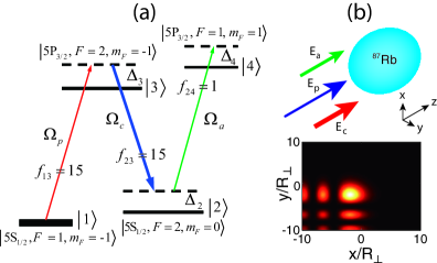
Figure 1: (Color online) (a) Energy-level diagram and excitation scheme of the lifetime-broadened four-state atomic system interacting with a weak pulsed probe field (with half Rabi frequency $\Omega_{p}$), a strong CW control field (with half Rabi frequency $\Omega_{c}$), and a weak CW assisted field (with half Rabi frequency $\Omega_{a}$). $\Delta_{3},$ $\Delta_{2}$, and $\Delta_{4}$ are one-photon, two-photon, and three-photon detunings, respectively. The energy levels are taken from the D₂ line of ⁸⁷Rb atoms, with $|1\rangle=|5{\rm S}_{1/2},F=1,m_{F}=-1\rangle$, $|2\rangle=|5{\rm S}_{1/2},F=2,m_{F}=0\rangle$, $|3\rangle=|5{\rm P}_{3/2},F=2,m_{F}=-1\rangle$, and $|4\rangle=|5{\rm P}_{3/2},F=1,m_{F}=1\rangle$. $f_{ij}=|\textbf{p}_{ij}/D2|^{2}\times 120$ is the relative transition strength, with $D2=3.58\times 10^{-27}$ cm C and $\textbf{p}_{ij}$ being the dipole transition matrix element between the state $|i\rangle$ and the state $|j\rangle$. (b) The geometry of the system. The lower part shows the intensity pattern of the assisted field, chosen as an Airy beam, in the $x$-$y$ plane.

A weak, pulsed probe field (strong, continuous-wave (CW) control field) with angular frequency $\omega_{p}$ ($\omega_{c}$) and wavevector $\textbf{k}_{p}$  ($\textbf{k}_{c}$) interacts resonantly with the energy states $|1\rangle$ and $|3\rangle$ ($|2\rangle$ and $|3\rangle$). In addition, a weak assisted laser field with angular frequency $\omega_{a}$ and wavevector $\textbf{k}_{a}$ couples to energy states $|2\rangle$ and $|4\rangle$, which contributes a cross-phase modulation (CPM) to the probe field, as shown below. The energy levels can be selected from the D₂ line of ⁸⁷Rb atoms, with the states assigned as $|1\rangle=|5{\rm S}_{1/2},F=1,m_{F}=-1\rangle$, $|2\rangle=|5{\rm S}_{1/2},F=2,m_{F}=0\rangle$, $|3\rangle=|5{\rm P}_{3/2},F=2,m_{F}=-1\rangle$, and $|4\rangle=|5{\rm P}_{3/2},F=2,m_{F}=1\rangle$ (see Fig. 1). In the figure, $f_{ij}$ is the relative transition strength, defined by $f_{ij}=|\textbf{p}_{ij}/D2|^{2}\times 120$. Here $D2=3.58\times 10^{-27}$ cm C and $\textbf{p}_{ij}$ is the dipole transition matrix element between the state $|i\rangle$, and the state $|j\rangle$ steck . The electric-field vector in the system can be written as $\textbf{E}=\sum_{l=p,c,a}\textbf{e}_{l}{\cal E}_{l}\exp{[i(\textbf{k}_{l}\cdot\textbf{r}-\omega_{l}t)]}+{\rm c.c.},$ where $\textbf{e}_{l}$ is polarization direction of $l$th field with envelope ${\cal E}_{l}$. The geometry of the system is illustrated in Fig. 1(b).

Under electric-dipole and rotating-wave approximations, the Hamiltonian in the interaction picture reads $\hat{H}_{\rm int}=-\hbar\sum_{j=1}^{4}\Delta_{j}|j\rangle\langle j|-\hbar(\Omega_{p}|3\rangle\langle 1|+\Omega_{c}|3\rangle\langle 2|+\Omega_{a}|4\rangle\langle 2|+{\rm H.c.}),$ where $\Delta_{3}=\omega_{p}-(\omega_{3}-\omega_{1}),$ $\Delta_{2}=\omega_{p}-\omega_{c}-(\omega_{2}-\omega_{1}),$ and $\Delta_{4}=\omega_{p}-\omega_{c}+\omega_{a}-(\omega_{4}-\omega_{1})$ are respectively the one-, two-, and three-photon detunings. $\Omega_{p}=(\textbf{e}_{p}\cdot\textbf{p}_{13}){\cal E}_{p}/\hbar$, $\Omega_{c}=(\textbf{e}_{c}\cdot\textbf{p}_{23}){\cal E}_{c}/\hbar$, and $\Omega_{a}=(\textbf{e}_{a}\cdot\textbf{p}_{24}){\cal E}_{a}/\hbar$ are respectively half Rabi frequencies of the probe, control, and assisted fields.

The equation of motion for the density-matrix $\sigma$ reads

$$\frac{\partial\sigma}{\partial t}=-\frac{i}{\hbar}\left[\hat{H}_{\rm int},\sigma\right]-\Gamma\sigma,$$ (1)

where $\Gamma$ is a $4\times 4$ relaxation matrix. Explicit expressions of the equations of motion for $\sigma_{ij}$ have been given in the Appendix A.

Electric-field evolution is controlled by Maxwell equation $\nabla^{2}\textbf{E}-(1/c^{2})\partial^{2}\textbf{E}/\partial t^{2}=(1/\epsilon_{0}c^{2})\partial^{2}\textbf{P}/\partial t^{2}$, with $\textbf{P}=N\{\textbf{p}_{13}\sigma_{31}\exp[i(\textbf{k}_{p}\cdot\textbf{r}-\omega_{p}t)]+\textbf{p}_{23}\sigma_{32}\exp[i(\textbf{k}_{c}\cdot\textbf{r}-\omega_{c}t)]+\textbf{p}_{24}\sigma_{42}\exp[i(\textbf{k}_{a}\cdot\textbf{r}-\omega_{a}t)]+{\rm c.c.}\}$. Under a slowly varying envelope approximation, we obtain the equations for $\Omega_{p}$ and $\Omega_{a}$:

$$i\left(\frac{\partial}{\partial z}+\frac{1}{c}\frac{\partial}{\partial t}\right)\Omega_{p}+\frac{c}{2\omega_{p}}\left(\frac{\partial^{2}}{\partial x^{2}}+\frac{\partial^{2}}{\partial y^{2}}\right)\Omega_{p}+\kappa_{13}\sigma_{31}=0,$$ (2a)

$$i\frac{\partial}{\partial z}\Omega_{a}+\frac{c}{2\omega_{a}}\left(\frac{\partial^{2}}{\partial x^{2}}+\frac{\partial^{2}}{\partial y^{2}}\right)\Omega_{a}+\kappa_{24}\sigma_{42}=0,$$ (2b)

where $\kappa_{13,24}=N\omega_{p,a}|\textbf{e}_{p,a}\cdot\textbf{p}_{13,24}|^{2}/(2\epsilon_{0}\hbar c)$, with $N$ being atomic concentration. For simplicity, the probe field and the assisted field have been assumed to propagate in $z$-direction, i.e. $\textbf{k}_{p,a}=\textbf{e}_{z}k_{p,a}$.

II.2 Asymptotic expansion and nonlinear envelope equations

Because we are interested in the nonlinear evolution and the possible formation of optical solitons in the system, we employ the standard method of multiple-scales, to investigate the evolution of both the probe and assisted fields. The atoms are assumed to be initially populated in the state $|1\rangle$. We make the asymptotic expansions $\sigma_{ij}=\sigma_{ij}^{(0)}+\epsilon\sigma_{ij}^{(1)}+\epsilon^{2}\sigma_{ij}^{(2)}+\epsilon^{3}\sigma_{ij}^{(3)}+\cdots$, and $\Omega_{p,a}=\epsilon\Omega_{p,a}^{(1)}+\epsilon^{2}\Omega_{p,a}^{(2)}+\epsilon^{3}\Omega_{p,a}^{(3)}+\cdots$, with $\sigma_{ij}^{(0)}=\delta_{i1}\delta_{j1}$ (both $\delta_{i1}$ and $\delta_{j1}$ are Kronecker delta symbols). Here $\epsilon$ is a small parameter characterizing the typical amplitude of the probe and assisted fields. To obtain divergence-free expansions, all quantities on the right hand sides of the asymptotic expansions are considered as functions of the multi-scale variables $z_{l}=\epsilon^{l}z$ ($l=0,1,2$), $t_{l}=\epsilon^{l}t$ ($l=0,2$), $x_{1}=\epsilon x$, and $y_{1}=\epsilon y$. Substituting these expansions into Eqs. (22) and (2), one can obtain a series of linear but inhomogeneous equations for $\sigma_{ij}^{(l)}$ and $\Omega_{p,a}^{(l)}$ ($l=1,2,3,...$), which can be solved order by order.

At the first-order, we obtain the solution under linear level:

$$\Omega_{p}^{(1)}=F\,e^{i\theta},\,\,\Omega_{a}^{(1)}=G,$$ (3a)

$$\sigma_{j1}^{(1)}=\frac{-\delta_{j2}\Omega_{c}^{\ast}+\delta_{j3}(\omega+d_{21})}{D}Fe^{i\theta},\,\,(j=2,3)$$ (3b)

with $D=|\Omega_{c}|^{2}-(\omega+d_{21})(\omega+d_{31})$, and other $\sigma_{ij}^{(1)}$ being zero. In the above expressions, $\theta=K(\omega)z_{0}-\omega t_{0}$, $F$ and $G$ are yet to be determined envelope functions depending on the slowly-varying variables $t_{2}$, $z_{1}$, and $z_{2}$. We see that in this order the two weak fields evolve independently. Moreover, the assisted field is free, but the probe field experiences a dispersion and absorption obeying the linear dispersion relation:

$$K(\omega)=\frac{\omega}{c}+\kappa_{13}\frac{\omega+d_{21}}{D}.$$ (4)

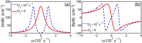
Figure 2: (Color online) The imaginary part Im$K(\omega)$ (panel (a) ) and the real part Re$K(\omega)$ (panel (b) ) of the linear dispersion relation $K(\omega)$ of the probe field as functions of $\omega$. In both panels, the dashed and solid lines correspond to the presence ($\Omega_{c}=1.0\times 10^{7}$ s^-1) and the absence ($\Omega_{c}=0$) of the control field, respectively. The other parameters are given in the text. A transparency window is opened for large control field (the dashed line in panel (a) ). The steep slope of the dashed-dotted line for large control field (the dashed line in panel (b) ) results in a ultraslow group velocity.

Shown in Fig. 2 is the imaginary part Im$K(\omega)$ (Fig. 2(a) ) and the real part Re$K(\omega)$ (Fig. 2(b) ) of $K(\omega)$ as functions of frequency $\omega$. As an example, we take the system parameters as $\Gamma_{12}\approx 1\,{\rm kHz},\,\Gamma_{13}\approx\Gamma_{23}\approx 6\,{\rm MHz},\,\Delta_{2,3}=0$ s${}^{-1},$ and $\kappa_{13}=1.0\times 10^{9}\,{\rm cm}^{-1}{\rm s}^{-1}.$ The dashed and the solid lines in both panels correspond to the presence ($\Omega_{c}=1.0\times 10^{7}$ s^-1) and the absence ($\Omega_{c}=0$) ) of the control field, respectively. One sees that when $\Omega_{c}$ is absent, the probe field has a large absorption (the solid line of Fig. 2(a) ); however, when $\Omega_{c}$ is applied an EIT transparency window is opened (the dashed line of Fig. 2(a) ). The steep slope for large control field (the dashed line of Fig. 2(b) ) results in a slow group velocity at the center frequency of the probe field (i.e. $\omega=0$ note1 ). The suppression of the absorption and the reduction of the group velocity are due to the EIT effect induced by the control field.

At the second-order, the solvability condition for $\sigma_{ij}^{(2)}$ and $\Omega_{p,a}^{(2)}$ requires $\partial F/\partial z_{1}=0$ and $\partial G/\partial z_{1}=0$, and hence both $F$ and $G$ are independent of $z_{1}$. At the third-order, using the solvability condition for $\sigma_{ij}^{(3)}$ and $\Omega_{p,a}^{(3)}$ we obtain the coupled nonlinear equations for $F$ and $G$:

$$i\left(\frac{\partial}{\partial z_{2}}+\frac{1}{V_{g}}\frac{\partial}{\partial t_{2}}\right)F+\frac{c}{2\omega_{p}}\left(\frac{\partial^{2}}{\partial x_{1}^{2}}+\frac{\partial^{2}}{\partial y_{1}^{2}}\right)F+\alpha_{11}|F|^{2}F+\alpha_{12}|G|^{2}F=0,$$ (5a)

$$i\frac{\partial}{\partial z_{2}}G+\frac{c}{2\omega_{a}}\left(\frac{\partial^{2}}{\partial x_{1}^{2}}+\frac{\partial^{2}}{\partial y_{1}^{2}}\right)G+\alpha_{21}|F|^{2}G=0,$$ (5b)

where $V_{g}=({\partial K}/{\partial\omega})^{-1}$ is the group velocity of the envelope $F$. The explicit expressions for the coefficient of self-phase modulation (SPM) of the probe field (i.e. $\alpha_{11}$), and the CPM coefficients between the two fields (i.e. $\alpha_{12}$ and $\alpha_{21}$), have been given in the Appendix B.

Since the selected atomic transition between $|2\rangle$ and $|4\rangle$ is much weak than those between $|1\rangle$ and $|3\rangle$ and between $|2\rangle$ and $|3\rangle$, the coupling constants in Eq. (2) satisfy $\kappa_{24}\ll\kappa_{13}$, and hence $\alpha_{21}\ll\alpha_{11},\alpha_{12}$. In this way the CPM term in Eq. (5b) can be safely neglected. Under this condition, Eq. (5b) is reduced into a linear Helmholtz equation. As a result, we obtain the following envelope equations

$$i\left(\frac{\partial}{\partial z}+\frac{1}{V_{g}}\frac{\partial}{\partial t}\right)U+\frac{c}{2\omega_{p}}\left(\frac{\partial^{2}}{\partial x^{2}}+\frac{\partial^{2}}{\partial y^{2}}\right)U+\alpha_{11}|U|^{2}U+\alpha_{12}|V|^{2}U=0,$$ (6a)

$$i\frac{\partial V}{\partial z}+\frac{c}{2\omega_{a}}\left(\frac{\partial^{2}}{\partial x^{2}}+\frac{\partial^{2}}{\partial y^{2}}\right)V=0,$$ (6b)

after returning to the original variables, where $U=\epsilon F$ and $V=\epsilon G$. One sees that the role of the assisted-field envelope $V$ is now acting as an external potential (controlled by Eq. (6b) ) to the probe field envelope $U$ (controlled by Eq. (6a) ). This is desirable because the external potential $|V|^{2}$ can be used not only to stabilize the motion of $U$ but also to guide it along a particular path, as shown below.

III Guiding ultraslow weak-light bullets with Airy beams

III.1 Estimation on the coefficients in the nonlinear envelope equations

Before solving Eqs. (6a) and (6b), we first make an estimation on their coefficients by using realistic physical parameters. Equations (6a) and (6b) can be written into the dimensionless form

$$i\left(\frac{\partial}{\partial s}+\lambda\frac{\partial}{\partial\tau}\right)u+\frac{1}{2}\left(\frac{\partial^{2}}{\partial\xi^{2}}+\frac{\partial^{2}}{\partial\eta^{2}}\right)u+g_{11}|u|^{2}u+g_{12}v_{0}^{2}|v|^{2}u=0,$$ (7a)

$$i\frac{\partial v}{\partial s}+\frac{\delta}{2}\left(\frac{\partial^{2}}{\partial\xi^{2}}+\frac{\partial^{2}}{\partial\eta^{2}}\right)v=0,$$ (7b)

where $u=U/U_{0}$, $v=V/(U_{0}v_{0})$, $s=z/L_{\rm diff}$, $\lambda=L_{\rm Diff}/(V_{g}\tau_{0})$, $\tau=t/\tau_{0}$ (with $\tau_{0}$ being the typical probe pulse length), $(\xi,\eta)=(x,y)/R_{\perp}$ (with $R_{\perp}$ being the typical probe beam radius), $g_{11}=\ell\alpha_{11}/|\alpha_{11}|$, $g_{12}=\ell\alpha_{12}/|\alpha_{11}|$, and $\delta=\omega_{p}/\omega_{a}$. Here $\ell=L_{\rm Diff}/L_{\rm NL}$, with $L_{\rm Diff}\equiv\omega_{p}R_{\perp}^{2}/c$ being the typical diffraction length, $L_{\rm NL}=1/(|\alpha_{11}U_{0}^{2}|)$ being the typical nonlinear length, and $U_{0}$ being the typical Rabi frequency of the probe field. The typical Rabi frequency of the probe field can be solved as $U_{0}=\sqrt{c/(\omega_{p}R_{\perp}^{2}|\alpha_{11}|)}$ if we take $\ell=1$, i.e. take $L_{\rm Diff}=L_{\rm NL}$. $v_{0}$ is proportional to the typical Rabi frequency of the assisted field, which is a free parameter that can be used to adjust the magnitude of the CPM coefficient, and hence control the stability of $U$.

Because the system we consider is lifetime-broadened, the coefficients in the Eq. (7a) are generally complex. If the control field Rabi frequency $\Omega_{c}$ is small, the imaginary part of the coefficients is comparable with their real part, and hence stable light bullet solutions do not exist. However, under EIT condition $|\Omega_{c}|^{2}\gg\gamma_{31}\gamma_{21}$ lil the absorption of the probe field can be largely suppressed, and hence the imaginary part of these coefficients can be made to be much smaller than their real part.

To show this we calculate the values of coefficients in the Eqs. (7a) and (7b) by considering a cold atomic gas of ⁸⁷Rb atoms, with ${\rm D}_{2}$ line transitions $5^{2}{\rm S}_{1/2}\rightarrow 5^{2}{\rm P}_{3/2}$. The energy levels are chosen as those in Fig. 1. From the data of ⁸⁷Rb steck , we have the dipole matrix elements $|\textbf{p}_{13}|\approx|\textbf{p}_{23}|=-\sqrt{\frac{1}{8}}\times 3.58\times 10^{-27}$ cm C and $|\textbf{p}_{24}|=\sqrt{\frac{1}{120}}\times 3.58\times 10^{-27}$ cm C. The other system parameters are taken as $\Gamma_{12}=1\,{\rm kHz}$, $\Gamma_{13}\approx\Gamma_{23}\approx\Gamma_{24}/2=35\,\,{\rm MHz}$, $\kappa_{13}=1.0\times 10^{10}\,\,{\rm cm}^{-1}{\rm s}^{-1}$, $\kappa_{24}=1.0\times 10^{9}\,\,{\rm cm}^{-1}{\rm s}^{-1}$, $\Omega_{c}=5.0\times 10^{7}\,{\rm s}^{-1}$, $\Delta_{2}=-1.5\times 10^{6}$ s^-1, $\Delta_{3}=-3.0\times 10^{8}\,{\rm s}^{-1}$, $\Delta_{4}=-1.0\times 10^{9}$ s^-1, $R_{\perp}=4.0\times 10^{-3}\,{\rm cm}$, and $U_{0}=9.0\times 10^{6}$ s^-1. Then we have $\delta\approx 1.0$, $g_{11}\approx 1.0-0.018i$, $g_{12}\approx 0.59-0.005i$, $g_{21}\approx 0.06+0.001i$, $L_{\rm Diff}=L_{\rm NL}\approx 1.26$ cm, and the group velocity

$$V_{g}\approx 5.6\times 10^{-6}\,c.$$ (8)

It is clear that the imaginary parts of the coefficients in Eqs. (7a) and (7b) are indeed much less than its real parts. The physical reason of so small imaginary part is due to the EIT effect induced by the control field that makes the absorption of the probe field largely suppressed. In the following discussion, the small imaginary parts of the coefficients are neglected for analytical analysis, but they are accounted in numerical simulations.

Note that Eq. (7a) is valid only for the probe filed with a large pulse length $\tau_{0}$ for which group-velocity dispersion effect of the system can be neglected. To estimate the required order of magnitude of $\tau_{0}$, we compare the characteristic dispersion length (defined by $L_{\rm Disp}={\rm Re}(\tau_{0}^{2}/|\partial^{2}K/\partial\omega^{2}|_{\omega=0}$) and the diffraction length $L_{\rm Diff}$ defined above. By setting $L_{\rm Disp}=L_{\rm Diff}$ we obtain $\tau_{0}=1.48\times 10^{-6}$ s. Consequently, if $\tau_{0}$ is much larger than $1.48\times 10^{-6}$ s, $L_{\rm Disp}$ will be much longer than $L_{\rm Diff}$ and hence the group-velocity dispersion effect of the system can be neglected safely.

III.2 Guiding a linear light bullet with one Airy beam

We first study the possibility of guiding a 3D linear light bullet with one Airy beam. If $U_{0}$ is much smaller than $9.0\times 10^{6}$ s^-1, the typical nonlinear length $L_{\rm NL}$ will be much longer than the typical diffraction length $L_{\rm Diff}$, and hence $\ell\ll 1$. Thus, the SPM term in the Eq. (7a) can be neglected because $g_{11}\propto\ell\ll 1$. However, the condition $\ell\ll 1$ will also suppress the CPM term which contributes to the trapping potential to the probe field. Without the potential, if a light bullet is excited, it will be highly unstable due to the transverse instability mal ; kiv . In addition, the potential will also be used to guide the light bullet. In order to avoid the suppression of the CPM term, we can use a large $v_{0}$ to fulfill the condition $\ell v_{0}^{2}\sim 1$. Taking into account the above considerations, Eq. (7a) reduces to a (3+1)D linear Schrödinger equation with a linear potential to the probe field.

Now we turn to the Helmholtz equation (7b). As we know, it admits different types of centrosymmetric beam solutions such as Gaussian beam, Bessel beam, and Laguerre-Gaussian beam Hall ; han3 , etc. However, in this work we are interested in a particular type of anticentrosymmetric beam solution, i.e. the Airy beam, with the form $v(s,\xi,\eta)={\rm Ai}(\xi-s^{2}/4){\rm Ai}(\eta-s^{2}/4)e^{i(\xi/2+\eta/2-s^{2}/6)s}$ Berry . At the entrance of the medium $v(0,\xi,\eta)={\rm Ai}(\xi){\rm Ai}(\eta)$ which can be experimentally realized by a Gaussian beam passing through a third-order phase mask. The Airy beam solution has many striking features. In particular, the intensity profile of its transverse part remains invariant (i.e. it does not spread out) when bending along a parabolic trajectory. However, the Airy beam is not square integrable (i.e. $\int Ai^{2}(x)dx\rightarrow\infty$). One possible way to solve this problem is to introduce an exponential aperture function, i.e. $v(0,\xi,\eta)={\rm Ai}(\xi){\rm Ai}(\eta)e^{a_{1}\xi+a_{2}\eta}$ Siviloglou1 ; Siviloglou2 . Here $a_{j}$ ($j=1,\,2$) are positive parameters introduced to ensure containment of the infinite Airy tail. Typically, $a_{j}\ll 1$ so that the resulting profile closely resembles the intended Airy function. By directly integrating Eq. (7b) we have

$$v(s,\xi,\eta) = {\rm Ai}(\xi-s^{2}/4+ia_{1}\xi){\rm Ai}(\eta-s^{2}/4+ia_{2}\xi)e^{i(\xi/2+\eta/2-s^{2}/6)s}$$ (9)

$$\times e^{a_{1}\xi-a_{1}\xi^{2}/2+ia_{1}^{2}\xi/2}e^{a_{2}\eta-a_{2}\eta^{2}/2+ia_{2}^{2}\eta/2}.$$

It is clear that the center position of the Airy beam (9) moves along the trajectory $\xi=\eta=s^{2}/4$, and hence tends to bend itself in transverse directions (i.e. the $x$ and $y$ directions).

Substituting the solution (9) into Eq. (7a) without the SPM term, we obtain the equation

$$i\left(\frac{\partial}{\partial s}+\lambda\frac{\partial}{\partial\tau}\right)u+\frac{1}{2}\left(\frac{\partial^{2}}{\partial\xi^{2}}+\frac{\partial^{2}}{\partial\eta^{2}}\right)u+g_{12}v_{0}^{2}|{\rm Ai}(\xi-s^{2}/4+ia_{1}\xi)$$

$$\times{\rm Ai}(\eta-s^{2}/4+ia_{2}\xi)|^{2}e^{2a_{1}\xi-a_{1}\xi^{2}}e^{2a_{2}\eta-a_{2}\eta^{2}}u=0.$$ (10)

We see that the Airy beam provides an “external potential” to the probe field. Equation (III.2) can be solved by taking han1 ; han2

$$u(\tau,\xi,\eta,s)=\phi(\tau,s)\psi(\tau,\xi,\eta),$$ (11)

with

$$\phi(\tau,s)=\frac{1}{\sqrt[4]{2\pi\rho^{2}}}e^{-(s-\tau/\lambda)^{2}/(4\rho^{2})}=\frac{1}{\sqrt[4]{2\pi\rho^{2}}}e^{-(z-V_{g}t)^{2}/(4\rho^{2}L_{\rm Diff}^{2})},$$ (12)

where $\rho$ is a free real parameter. When writing Eq. (12) we have assumed that the probe-field envelope is a Gaussian pulse propagating in $z$ direction with velocity $V_{g}$. In this way, the transverse distribution $\psi(\tau,\xi,\eta)$ satisfies the linear equation

$$i\lambda\frac{\partial\psi}{\partial\tau}+\frac{1}{2}\left(\frac{\partial^{2}}{\partial\xi^{2}}+\frac{\partial^{2}}{\partial\eta^{2}}\right)\psi+g_{12}v_{0}^{2}|{\rm Ai}(\xi-s^{2}/4+ia_{1}\xi){\rm Ai}(\eta-s^{2}/4+ia_{2}\xi)|^{2}$$

$$\times e^{2a_{1}\xi-a_{1}\xi^{2}}e^{2a_{2}\eta-a_{2}\eta^{2}}\psi=0,$$ (13)

and its stationary solutions can be obtained by the transformation $\psi=\exp{(i\mu\tau)}\tilde{\psi}(\xi,\eta)$, leading to the linear eigenvalue equation

$${\cal L}\tilde{\psi}=\lambda\mu\tilde{\psi},\\$$ (14)

with the operator

$${\cal L}=\frac{1}{2}\left(\frac{\partial^{2}}{\partial\xi^{2}}+\frac{\partial^{2}}{\partial\eta^{2}}\right)+g_{12}v_{0}^{2}|{\rm Ai}(\xi+ia_{1}\xi){\rm Ai}(\eta+ia_{2}\xi)|^{2}e^{2a_{1}\xi-a_{1}\xi^{2}}e^{2a_{2}\eta-a_{2}\eta^{2}},$$

where $\tilde{\psi}$ is a real function and $\mu$ is the propagation constant. If $\tilde{\psi}$ is transversely localized, $u$ will be localized in all three spatial directions and evolve in time. In this way, $u$ will describe a linear light bullet in (3+1)D.

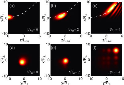
Figure 3: (Color online) Guiding a linear light bullet with Airy beam ($U_{0}=1.8\times 10^{-6}$ s^-1). (a)-(c) Intensity patterns of the linear light bullet in the $x$-$z$ plane at $\tau/\tau_{0}=0$, 2, and 4, respectively. Dashed lines denote the trajectory of the main lobe of the Airy potential. (d)-(f) Intensity patterns of the linear light bullet in the $x$-$y$ plane at $\tau/\tau_{0}=0$, 2, and 4, respectively. A significant diffraction can be observed in (c) and (f).

In Fig. 3 we show the guiding of a typical linear light bullet with the assisted field taken to be an Airy beam. Fig. 3(a) and Fig. 3(d) show the intensity pattern of the linear light bullet by solving Eq. (14). Here we have taken $\tau_{0}=7.5\times 10^{-6}$ s so that $\lambda=1$. To test the stability of the linear light bullet, we calculate the power of the probe pulse, defined by $P=2\pi\iiint_{-\infty}^{+\infty}\psi^{2}d\xi d\eta d\tau$, as a function of the propagation constant $\mu$. For a given $v_{0}$, $P$ first increases to arrive a maximum, and then decreases. According to Vakhitov-Kolokolov (VK) criterion vakhitov1 , the domain in which the linear light bullet is stable is the one with $dP/d\mu>0$. Generally, the stability domain is small for small $v_{0}$, however, it can be enlarged by increasing $v_{0}$. This is because a larger $v_{0}$ means a stronger trapping to the optical pulse provided by the potential. In our calculation, the stability domain is $0<\mu\lesssim 0.6$ with $v_{0}=23$.

The guiding of such linear light bullet is studied by making simulation of Eq. (III.2) with the stationary solution in Fig. 3(a) and Fig. 3(d) as the initial condition. The results are presented in Fig. 4(b) and Fig. 4(c) (Fig. 4(e) and Fig. 4(f) ) at $\tau/\tau_{0}=2$ and 4, respectively. We see that the linear light bullet is indeed guided by the Airy-shaped assisted field. Specifically, it is trapped in the main lobe of the Airy beam, propagate ultraslowly in longitudinal direction, accelerate in transverse directions, and move along a parabolic trajectory. However, the linear light bullet is unstable because a significant diffraction occurs during the propagation, which makes it spread along the parabolic trajectory and leak energy to the other lobes of the Airy beam (see Fig. 4(c) and Fig. 4(f) ).

III.3 Guiding nonlinear light bullets with one Airy beam

Since the diffraction-induced spreading occurs during the propagation of the linear light bullet, a natural idea is to use the SPM effect of the system to balance the diffraction. To have a significant SPM, one must increase the amplitude of the probe field. By taking $U_{0}=9.0\times 10^{6}$ s^-1 (five times larger than that in the linear case), we have $g_{11}\approx 1$ and hence the SPM term plays an important role in the Eq. (7a). Substituting the solution (9) into Eq. (7a), we obtain the (3+1)D nonlinear Schrödinger (NLS) equation

$$i\left(\frac{\partial}{\partial s}+\lambda\frac{\partial}{\partial\tau}\right)u+\frac{1}{2}\left(\frac{\partial^{2}}{\partial\xi^{2}}+\frac{\partial^{2}}{\partial\eta^{2}}\right)u+g_{11}|u|^{2}u+g_{12}v_{0}^{2}|{\rm Ai}(\xi-s^{2}/4+ia_{1}\xi)$$

$$\times{\rm Ai}(\eta-s^{2}/4+ia_{2}\xi)|^{2}e^{2a_{1}\xi-a_{1}\xi^{2}}e^{2a_{2}\eta-a_{2}\eta^{2}}u=0.$$ (15)

With (11) and (12), we have

$$i\lambda\frac{\partial\psi}{\partial\tau}+\frac{1}{2}\left(\frac{\partial^{2}}{\partial\xi^{2}}+\frac{\partial^{2}}{\partial\eta^{2}}\right)\psi+g_{11}|\psi|^{2}\psi+g_{12}v_{0}^{2}|{\rm Ai}(\xi-s^{2}/4+ia_{1}\xi){\rm Ai}(\eta-s^{2}/4+ia_{2}\xi)|^{2}$$

$$\times e^{2a_{1}\xi-a_{1}\xi^{2}}e^{2a_{2}\eta-a_{2}\eta^{2}}\psi=0.$$ (16)

Similarly, the stationary solutions of Eq. (III.3) can be obtained by the transformation $\psi=\exp{(i\mu\tau)}\tilde{\psi}(\xi,\eta)$, leading to the nonlinear eigenvalue equation

$${\cal L}\tilde{\psi}+g_{11}\tilde{\psi}^{3}=\lambda\mu\tilde{\psi},\\$$ (17)

where the operator ${\cal L}$ is the same with that defined in Eq. (14).

Fig. 4(a) and Fig. 4(d) show the intensity pattern of a stationary nonlinear light bullet by solving Eq. (17). The values of $\tau_{0}$ and $\rho$ are the same with those used in the last subsection. For a given $v_{0}$, the probe-field power $P$ first increases to arrive a maximum, and then decreases. However, the stability domain of a nonlinear light bullet is larger than that of a linear one. This is because the focusing nonlinearity favors to the formation of the nonlinear light bullet, and hence enhances its stability. For example, the stability domain is $0<\mu\lesssim 1.5$ for $v_{0}=7.3$.

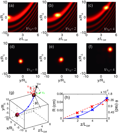
Figure 4: (Color online) Guiding nonlinear light bullet with Airy beam. (a)-(c) Intensity patterns of the nonlinear light bullet in the $x$-$z$ plane at $\tau/\tau_{0}=0$, 2, and 4, respectively. (d)-(f) Intensity patterns of the nonlinear light bullet in the $x$-$y$ plane at $\tau/\tau_{0}=0$, 2, and 4. (g) Schematic diagram of the propagation of the nonlinear light bullet in three-dimensional space. $V_{x}$ ($V_{y}$) is the velocity in the $x$ ($y$) direction; $V_{r}=\sqrt{V_{x}^{2}+V_{y}^{2}}$ is the radial velocity in the $x$-$y$ plane; $V_{g}$ is the group velocity in the $z$ direction; $V_{\rm LB}=\sqrt{V_{r}^{2}+V_{g}^{2}}$ is the total velocity; $R$ is the transverse displacement after the nonlinear light bullet passing through the atomic medium; $\theta$ is the angle between $V_{r}$ and $V_{g}$; the (red) solid spheres represents the nonlinear light bullet. (h) $R$ and $\theta$ as functions of $z$. The solid and dashed lines are analytical results, the “$\times$” symbols are results by numerical simulations.

The guiding of the nonlinear light bullet is studied by making a numerical simulation of Eq. (III.3) with the stationary solution given in Fig. 4(a) and Fig. 4(d) as an initial condition. The results in Fig. 4(b) and Fig. 4(c) (Fig. 4(e) and Fig. 4(f) ) are for $\tau/\tau_{0}=2$ and 4, respectively. We see that the nonlinear light bullet is indeed guided by the Airy-beam-shaped assisted field. Importantly, different from the linear light bullet given in the last subsection no evident diffraction is observed during the propagation of the nonlinear light bullet. This is because the diffraction is completely balanced by the SPM effect even the trajectory of the nonlinear light bullet is bent.

The position of the nonlinear light bullet can be obtained by the trajectory of the main lobe of the Airy beam, which reads

$$(X,Y,Z)=\left(\frac{R_{\perp}V_{g}^{2}}{4L_{\rm Diff}^{2}}t^{2},\frac{R_{\perp}V_{g}^{2}}{4L_{\rm Diff}^{2}}t^{2},V_{g}t\right).$$ (18)

From Eq. (18) we see that the nonlinear light bullet accelerates in both $x$ and $y$ directions with the same accelerated velocity $R_{\perp}V_{g}^{2}/(2L_{\rm Diff}^{2})$, and propagates in $z$ direction with the constant propagating velocity $V_{g}$. In a mechanical point of view, the acceleration of the nonlinear light bullet is caused by the transverse force produced by the potential contributed by the assisted field.

For clearance, in Fig. 4(g) we show the schematic diagram for the propagation of the nonlinear light bullet in three-dimensional space. In this figure, $V_{x}$ and $V_{y}$ are respectively the velocities of the nonlinear light bullet in $x$ and $y$ directions, $V_{r}=\sqrt{V_{x}^{2}+V_{y}^{2}}$ is the radial velocity in the transverse plane, $V_{g}$ is the velocity in $z$ direction, $V_{\rm LB}=\sqrt{V_{r}^{2}+V_{g}^{2}}$ is the total velocity, $R$ is the transverse displacement after the light bullet passing through the atomic medium, and $\theta$ is the angle between $V_{r}$ and $V_{g}$ describing the output direction.

Shown in Fig. 4(h) are $R$ and $\theta$ as functions of $z$. The solid and dashed lines are analytical results, while “$\times$” symbols are results by making numerical simulation. We see that the position of the nonlinear light bullet can be controlled and manipulated by the Airy beam. For example, we obtain $R\approx 0.05$ cm and $\theta\approx 1.35\times 10^{-2}$ rad after the nonlinear light bullet passing through a medium with the length $6L_{\rm Diff}=7.56$ cm. We note that the magnitude of the output angle obtained here is one order larger than that obtained using a Stern-Gerlach gradient magnetic field in Ref. kar .

The generation power of the (3+1)D nonlinear light bullet described above can be estimated by calculating Poynting’s vector. The peak power of the probe field is given by $\bar{P}_{\rm{max}}=2\epsilon_{0}cn_{p}S_{0}(\hbar/|\textbf{ p}_{13}|)^{2}U_{0}^{2}|u_{\rm max}|^{2}$, with $n_{p}$ and $S_{0}$ being the reflective index and the cross-section area of the probe beam, respectively. Taking $S_{0}=\pi R_{\perp}^{2}\approx 0.5\times 10^{-4}$ cm² and using the other parameters given above, we obtain the generation power of the nonlinear light bullet

$$\bar{P}_{\rm{max}}\approx 1.8\,\,\mu{\rm W}.$$ (19)

Consequently, the nonlinear light bullet in the present system may have not only an ultraslow propagating velocity but also a very low generation power. This is fundamentally different from the other generation schemes where the light bullets have the propagating velocity of the same order of $c$ and their generation power up to megawatt is needed tra ; min .

III.4 Guiding nonlinear light bullets with two sequential Airy beams

In this subsection we show that if the assisted field is taken to be two sequential Airy beams, the nonlinear light bullet can easily bypass an obstacle. To this end, we assume that the assisted field takes the form

$$v(\tau,s,\xi,\eta) = \{f_{1}(\tau){\rm Ai}(\xi-s^{2}/4+ia_{1}\xi){\rm Ai}(\eta-s^{2}/4+ia_{2}\xi)e^{i(\xi/2+\eta/2-s^{2}/6)s}$$ (20)

$$+f_{2}(\tau){\rm Ai}[\xi-(s-s_{0})^{2}/4+ia_{1}\xi]{\rm Ai}[\eta-(s-s_{0})^{2}/4+ia_{2}\xi]$$

$$\times e^{i[\xi/2+\eta/2-(s-s_{0})^{2}/6](s-s_{0})}\}e^{a_{1}\xi-a_{1}\xi^{2}/2+ia_{1}^{2}\xi/2}e^{a_{2}\eta-a_{2}\eta^{2}/2+ia_{2}^{2}\eta/2},$$

where $f_{1}(\tau)=\frac{1}{2}\left\{1-\tanh[2(\tau-\tau_{1})]\right\}$ and $f_{2}(\tau)=\frac{1}{2}\left\{1+\tanh[2(\tau-\tau_{1})]\right\}$, with $s_{0}$ being the length of the medium. Clearly, the solution (21) obeys the Helmholtz equation (7b) because it is a combination of two sequential Airy beams, propagating respectively along $z$ and $-z$ directions in different time.

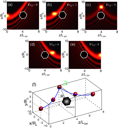
Figure 5: (Color online) Nonlinear light bullet bypasses an obstacle. (a)-(e) Intensity patterns of the nonlinear light bullet in the $x$-$z$ plane for $\tau/\tau_{0}=0$, 2, 4, 6, and 8, respectively. The black Polygone represents an obstacle. (f) The propagation of the nonlinear light bullet (represented by the (red) solid spheres) in the 3D space. The “$\Lambda$” shape trajectory of the nonlinear light bullet enables it to bypass the obstacle (represented by the black Polygone).

In Fig. 5(a)-Fig. 5(e) we show the intensity patterns of the nonlinear light bullet at $t/\tau_{0}=0$, 2, 4, 6, and 8, respectively, for $\tau_{1}=4$ and $s_{0}=8$. In the first time interval, i.e. $\tau\in(0,4)$, the nonlinear light bullet with initial position $(x,y,z)=(0,0,0)$ is trapped in the forward Airy beam (i.e. the beam with $f_{1}(\tau)\approx 1$, $f_{2}(\tau)\approx 0$) and moves along the main lobe of the beam to the position $(x,y,z)=(4R_{\perp},4R_{\perp},4L_{\rm Diff})$ at $\tau=4$, as shown in Fig. 5(c). In the second time interval, i.e. $\tau\in(4,8)$, the forward Airy beam is switched off and the backward Airy beam (i.e. the beam with $f_{1}(\tau)\approx 0$, $f_{2}(\tau)\approx 1$) is switched on. In this time interval, the nonlinear light bullet is trapped in the backward Airy beam and moves along the main lobe of the beam to the position $(x,y,z)=(4R_{\perp},4R_{\perp},8L_{\rm Diff})$ at $\tau=8$, as shown in Fig. 5(e). Interestingly, we see that the nonlinear light bullet travels along a “$\Lambda$” shape trajectory. Consequently, if there is an obstacle which is put in the position below the “$\Lambda$” shape trajectory, the nonlinear light bullet can bypass the obstacle, as shown in Fig. 5(f) (in all panels, the black Polygone represents the obstacle).

IV Generation of nonlinear helical light bullets

The Airy beam can also be used to generate an ultraslow helical weak-light bullet proposed in Ref. han2 . To this end, we assume that the assisted field takes the form

$$v(\tau,s,\xi,\eta) = f_{1}(\tau){\rm Ai}(\xi-s^{2}/4+ia_{1}\xi){\rm Ai}(\eta-s^{2}/4+ia_{2}\xi)e^{i(\xi/2+\eta/2-s^{2}/6)s}$$ (21)

$$\times e^{a_{1}\xi-a_{1}\xi^{2}/2+ia_{1}^{2}\xi/2}e^{a_{2}\eta-a_{2}\eta^{2}/2+ia_{2}^{2}\eta/2}+f_{2}(\tau)J_{1}(\sqrt{2b}r),$$

with $f_{1}(\tau)$ and $f_{2}(\tau)$ being the same with those defined in Eq. (20), $J_{1}$ being the first-order Bessel function, $b$ being a real constant characterizing the radius of the Bessel function, and $r=\sqrt{\xi^{2}+\eta^{2}}$. It is clear that the solution (21) also obeys the Helmholtz equation (7b) because it is a combination of Bessel and Airy beams which are both solutions of the Helmholtz equation.

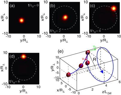
Figure 6: (Color online) Generating a nonlinear helical light bullet with Airy beam. (a)-(d) Intensity patterns of the nonlinear light bullet in the $x$-$y$ plane at $t/\tau_{0}=0$, 2, 4, and 6, respectively, for $\tau_{1}=4$ and $b=0.05$. (e) The propagation of the helical light bullet in 3D space. The solid line with arrow denotes the motion trajectory of the nonlinear light bullet. The radius of the ring $R\approx 5.66R_{\perp}$.

In Fig. 5(a)-Fig. 5(d) we show the intensity patterns of the light bullet at $t/\tau_{0}=0$, 2, 4, and 6, respectively, for $\tau_{1}=4$ and $b=0.05$. In the first time interval, $\tau\in(0,4)$, the nonlinear light bullet is trapped in the Airy beam and moves to the position $(x,y)=(4R_{\perp},4R_{\perp})$ at the end of the first interval, as shown in Fig. 6(c). After the first time interval, we switch off the Airy beam and switch on the first-order Bessel beam, the nonlinear light bullet is then trapped in the first ring of the first-order Bessel beam and moves along the ring if the trapping potential contributed by the ring is narrow and deep enough. This is possible because in each ring of the Bessel beam the potential energy is degenerate and reaches its minimum, therefore a light bullet will move along the ring if an initial transverse velocity $V_{t}$ tangent to the ring is given. Notice that after switching off the Airy beam the velocity of the light bullet in the transverse plane is the radial velocity $V_{r}$ which is orthogonal to the ring, and hence it can not trigger on the rotary motion when the first-order Bessel beam is switched on. However, a tangent velocity $V_{t}$ can be produced by various methods such as using a gradient magnetic field han2 or a shift of the Bessel lattice he . Then, the nonlinear light bullet rotates around the circle, as shown in Fig. 6(d).

Since now the nonlinear light bullet has two orthogonal velocities, the tangent velocity $V_{t}$ and the group velocity $V_{g}$, they can actually make a helical motion in the 3D space, as shown in Fig. 6(e), where the solid line with arrow denotes the motion trajectory of the nonlinear light bullet. Because both velocities are much smaller than $c$ and the generation power of the nonlinear light bullet is very weak, such light bullet is named as the ultraslow helical weak-light bullet.

In general, it is possible to move a nonlinear light bullet from the center of the transverse plane to any ring of Bessel lattices. By using such assisted field with sequential Airy and Bessel beams, one can manipulate and control the output position of a nonlinear light bullet in a very efficient way.

V Summary

In this article, we have studied the possibility of guiding stable ultraslow weak-light bullets by using Airy beams in a cold, lifetime-broadened four-level atomic system via EIT. We have shown that under the EIT condition the light bullet with ultraslow propagating velocity ($\sim 10^{-5}\,c$) and extremely low generation power ($\sim 1\,\mu W$) formed by the balance between diffraction and nonlinearity in the probe field can be not only stabilized but also guided by the assisted field. In particular, when the assisted field is taken to be an Airy beam the light bullet can be trapped into the main lobe of the Airy beam, propagate ultraslowly in longitudinal direction, accelerate in transverse directions, and hence move along a parabolic trajectory. We have demonstrated that the light bullet can bypass an obstacle by using two sequential Airy beams. A technique of generating ultraslow helical weak-light bullets in the present system has also been proposed. The results obtained in this work are useful for guiding new experimental findings and have potential applications in optical information processing and transmission. For instance, the guided light bullets suggested here can be used to design all-optical switching and logic gates. In addition, they can also be employed to design new type of all-optical routers for transmitting optical information.

Appendix A Equations of motion for $\sigma_{ij}$

Equations of motion for $\sigma_{ij}$ are given by

$$i\frac{\partial}{\partial t}\sigma_{11}-i\Gamma_{31}\sigma_{33}+\Omega_{p}^{\ast}\sigma_{31}-\Omega_{p}\sigma_{31}^{\ast}=0,$$ (22a)

$$i\frac{\partial}{\partial t}\sigma_{22}-i\Gamma_{32}\sigma_{33}-i\Gamma_{42}\sigma_{44}+\Omega_{c}^{\ast}\sigma_{32}-\Omega_{c}\sigma_{32}^{\ast}+\Omega_{a}^{\ast}\sigma_{42}-\Omega_{a}\sigma_{42}^{\ast}=0,$$ (22b)

$$i\left(\frac{\partial}{\partial t}+\Gamma_{3}\right)\sigma_{33}-\Omega_{p}^{\ast}\sigma_{31}+\Omega_{p}\sigma_{31}^{\ast}-\Omega_{c}^{\ast}\sigma_{32}+\Omega_{c}\sigma_{32}^{\ast}=0,$$ (22c)

$$i\left(\frac{\partial}{\partial t}+\Gamma_{4}\right)\sigma_{44}-\Omega_{a}^{\ast}\sigma_{42}+\Omega_{a}\sigma_{42}^{\ast}=0,$$ (22d)

$$\left(i\frac{\partial}{\partial t}+d_{21}\right)\sigma_{21}+\Omega_{c}^{\ast}\sigma_{31}+\Omega_{a}^{\ast}\sigma_{41}-\Omega_{p}\sigma_{32}^{\ast}=0,$$ (22e)

$$\left(i\frac{\partial}{\partial t}+d_{31}\right)\sigma_{31}+\Omega_{p}(\sigma_{11}-\sigma_{33})+\Omega_{c}\sigma_{21}=0,$$ (22f)

$$\left(i\frac{\partial}{\partial t}+d_{41}\right)\sigma_{41}+\Omega_{a}\sigma_{21}-\Omega_{p}\sigma_{43}=0,$$ (22g)

$$\left(i\frac{\partial}{\partial t}+d_{32}\right)\sigma_{32}+\Omega_{c}(\sigma_{22}-\sigma_{33})+\Omega_{p}\sigma_{21}^{\ast}-\Omega_{a}\sigma_{43}^{\ast}=0,$$ (22h)

$$\left(i\frac{\partial}{\partial t}+d_{42}\right)\sigma_{42}+\Omega_{a}(\sigma_{22}-\sigma_{44})-\Omega_{c}\sigma_{43}=0,$$ (22i)

$$\left(i\frac{\partial}{\partial t}+d_{43}\right)\sigma_{43}+\Omega_{a}\sigma_{32}^{\ast}-\Omega_{p}^{\ast}\sigma_{41}-\Omega_{c}^{\ast}\sigma_{42}=0,$$ (22j)

where $\Gamma_{ij}$ is the rate at which population decays from the state $|i\rangle$ to the state $|j\rangle$, $d_{ij}=\Delta_{i}-\Delta_{j}+i\gamma_{ij}$ with $\gamma_{ij}\equiv(\Gamma_{i}+\Gamma_{j})/2+\gamma^{{\rm dph}}_{ij}$. Here $\Gamma_{i}=\sum_{E_{j}<E_{i}}\Gamma_{ij}$ and $\gamma_{ij}^{\text{col}}$ denotes the dipole dephasing rate caused by atomic collisions.

Appendix B Explicit expressions of $\alpha_{jl}$

The explicit expressions of $\alpha_{jl}$ read

$$\alpha_{11}=\frac{\kappa_{13}}{D}\left\{\Omega_{c}a_{32}^{\ast(2)}-(\omega+d_{21})\left[\frac{4}{\Gamma_{31}}{\rm Im}\left(\frac{d_{21}}{D}\right)+a_{22}^{(2)}\right]\right\},$$ (23a)

$$\alpha_{12}=-\frac{\kappa_{13}|\Omega_{c}|^{2}}{(\omega+d_{41})D^{2}},$$ (23b)

$$\alpha_{21}=\frac{\kappa_{24}}{|\Omega_{c}|^{2}-d_{42}d_{43}}\left[d_{43}a_{22}^{(2)}+\Omega_{c}a_{32}^{\ast(2)}-\frac{|\Omega_{c}|^{2}}{(\omega+d_{41})D}\right],$$ (23c)

with

$$a_{22}^{(2)}=\left[\frac{2}{\Gamma_{31}}{\rm Im}\left(\frac{d_{21}}{D}\right)-\frac{{\rm Im}\left(\frac{1}{d_{32}^{\ast}D}\right)}{{\rm Im}\left(\frac{1}{d_{32}}\right)}-\frac{\Gamma_{32}}{\Gamma_{31}|\Omega_{c}|^{2}}\frac{{\rm Im}\left(\frac{d_{21}}{D}\right)}{{\rm Im}\left(\frac{1}{d_{32}}\right)}\right],$$ (24a)

$$a_{33}^{(2)}=\frac{2{\rm Im}\left(\frac{d_{21}}{D}\right)}{\Gamma_{31}}$$ (24b)

$$a_{32}^{(2)}=\frac{1}{d_{32}}\left[\frac{\Omega_{c}}{D^{\ast}}+\Omega_{c}(a_{33}^{(2)}-a_{22}^{(2)})\right].$$ (24c)

References

- (1) Y. Silberberg, Opt. Lett. 22, 1282 (1990).
- (2) L. Berge, Phys. Rep. 303, 260 (1998).
- (3) Y. S. Kivshar and D. E. Pelinovsky, Phys. Rep. 331, 117 (1998).
- (4) B. A. Malomed, D. Mihalache, F. Wise, and L. Torner, J. Phys. B: Quantum Semiclass. Opt. 7, R53 (2005), and references therein.
- (5) Y. S. Kivshar and G. P. Agrawal, Optical Solitons: From Fibers to Photonic Crystals (Academic Press, London, 2006), and references therein.
- (6) X. Liu, L. J. Qian and F. W. Wise, Phys. Rev. Lett. 82, 4631 (1999).
- (7) M. Blaauboer, B. A. Malomed, and G. Kurizki, Phys. Rev. Lett. 84, 1906 (2000).
- (8) I. N. Towers, B. A. Malomed, and F. W. Wise, Phys. Rev. Lett. 90, 123902 (2003).
- (9) P. D. Trapani, G. Valiulis, A. Piskarskas, O. Jedrkiewicz, J. Trull, C. Conti, and S. Trillo, Phys. Rev. Lett. 91, 093904 (2003).
- (10) D. Mihalache, D. Mazilu, F. Ledererm B. A. Malomed, Y. V. Kartashov, L.-C. Crasovan, and L. Torner, Phys. Rev. Lett. 95, 023902 (2005).
- (11) M. Matuszewski, E. Infeld, B. A. Malomed, and M. Trippenbach, Phys. Rev. Lett. 95, 050403 (2005).
- (12) L. Bergé and S. Skupin, Phys. Rev. Lett. 100, 113902 (2008).
- (13) M. Belić, N. Petrović, W. P. Zhong, R. H. Xie, and G. Chen, Phys. Rev. Lett. 101, 123904 (2008).
- (14) I. B. Burgess, M. Peccianti, G. Assanto, and R. Morandotti, Phys. Rev. Lett. 102, 203903 (2009).
- (15) S. H. Chen and J. M. Dudley, Phys. Rev. Lett. 102, 233903 (2009).
- (16) D. Abdollahpour, S. Suntsov, D. G. Papazoglou, and S. Tzortzakis, Phys. Rev. Lett. 105, 253901 (2010).
- (17) S. Minardi, F. Eilenberger, Y. V. Kartashov, A. Szameit, U. Röpke, J. Kobelke, K. Schuster, H. Bartelt, S. Nolte, L. Torner, F. Lederer, A. Tünnermann, and T. Pertsch, Phys. Rev. Lett. 105, 263901 (2010).
- (18) A. M. Mateo, V. Delgado, and B. A. Malomed, Phys. Rev. A 82, 053606 (2010).
- (19) Y. V. Kartashov, B. A. Malomed, and L. Torner, Rev. Mod. Phys. 83, 247 (2011).
- (20) D. Mihalache, D. Mazilu, F. Lederer, and Y. S. Kivshar, Opt. Lett. 32, 3173 (2007).
- (21) D. Mihalache, D. Mazilu, F. Lederer, and Y. S. Kivshar, Phys. Rev. A 79, 013811 (2009).
- (22) D. Mihalache, J. Opt. Adv. Mat. 12, 12 (2010).
- (23) S. E. Harris, Phys. Today 50(7), 36 (1997).
- (24) M. Fleischhauer, A. Imamoglu, and J. P. Marangos, Rev. Mod. Phys. 77, 633 (2005), and references therein.
- (25) Y. Wu and L. Deng, Phys. Rev. Lett. 93, 143904 (2004).
- (26) G. Huang, L. Deng and M. G. Payne, Phys. Rev. E. 72, 016617 (2005).
- (27) C. Hang and G. Huang, Phys. Rev. A 77, 033830 (2008).
- (28) W.-X. Yang, A.-X. Chen, L.-G. Si, K. Jiang, X. Yang, and R.-K. Lee, Phys. Rev. A 81, 023814 (2010).
- (29) T. Hong, Phys. Rev. Lett. 90, 183901 (2003).
- (30) H. Michinel and M. J. Paz-Alonso, Phys. Rev. Lett. 96, 023903 (2006).
- (31) C. Hang, G. Huang, and L. Deng, Phys. Rev. E 73, 046601 (2006).
- (32) C. Hang, V. V. Konotop, and G. Huang, Phys. Rev. A 79, 033826 (2009).
- (33) H. Li, Y. Wu, and G. Huang, Phys. Rev. A 84, 033816 (2009).
- (34) C. Hang and G. Huang, Phys. Rev. A 86, 043809 (2012).
- (35) C. Hang and G. Huang, Phys. Rev. A 87, 053809 (2013).
- (36) M. V. Berry and N. L. Balazs, Am. J. Phys. 47, 264 (1979).
- (37) M. A. Bandres, I. Kaminer, M. S. Mills, B. M. Rodriguez-Lara, E. Greenfield, M. Segev, and D. N. Christodoulides, Opt. & Photon. News 24, 30 (2013).
- (38) J. Baumgartl, M. Mazilu, and K. Dholakia, Nature Photonics 2, 675 (2008).
- (39) P. Zhang, J. Prakash, Z. Zhang, M. S. Mills, N. K. Efremidis, D. N. Christodoulides, and Z. Chen, Opt. Lett. 36, 2883 (2011).
- (40) P. Polynkin, M. Kolesik, J. V. Moloney, G. A. Siviloglou, and D. N. Christodoulides, Science 324, 229 (2009).
- (41) L. Li, T. Li, S. M. Wang, C. Zhang, and S. N. Zhu, Phys. Rev. Lett. 107, 126804 (2011).
- (42) Here the first ‘3’ refers to spatial coordinates and ‘1’ refers one time coordinate.
- (43) D. A. Steck, “Rubidium 87 D Line Data”, http://steck.us/alkalidata/.
- (44) The frequency and wavevector of the probe field is given by and . Thus corresponds to the center frequency of the probe field.
- (45) L. Li and G. Huang, Phys. Rev. A 82, 023809 (2010).
- (46) D. G. Hall, Opt. Lett. 21, 9 (1996).
- (47) C. Hang and V. V. Konotop, Phys. Rev. A 83, 053845 (2012).
- (48) G. A. Siviloglou and D. N. Christodoulides, Opt. Lett. 32, 979 (2007).
- (49) G. A. Siviloglou, J. Broky, A. Dogariu, and D. N. Christodoulides, Phys. Rev. Lett. 99, 213901 (2007).
- (50) M. G. Vakhitov and A. A. Kolokolov, Sov. J. Radiophys. Quantum Electron. 16, 783 (1973).
- (51) L. Karpa and M. Weitz, Nat. Phys. 2, 332 (2006).
- (52) Y. J. He, Boris A. Malomed, and H. Z. Wang, Phys. Rev. A 76, 053601 (2007).