Lyapunov spectrum for Hénon-like maps
at the first bifurcation

Abstract.

For a strongly dissipative Hénon-like map at the first bifurcation parameter at which the uniform hyperbolicity is destroyed by the formation of tangencies inside the limit set, we effect a multifractal analysis, i.e., decompose the set of non wandering points on the unstable manifold into level sets of an unstable Lyapunov exponent, and give a partial description of the Lyapunov spectrum which encodes this decomposition. We derive a formula for the Hausdorff dimension of the level sets in terms of the entropy and unstable Lyapunov exponent of invariant probability measures, and show the continuity of the Lyapunov spectrum. We also show that the set of points for which the unstable Lyapunov exponents do not exist carries a full Hausdorff dimension.

1. introduction

In the study of chaotic dynamical systems, one often encounters invariant sets with complicated geometric structures. The multifractal analysis treats the so-called multifractal decomposition of these sets, and the associated multifractal spectrum which encodes the decomposition. The goal is to relate the spectrum to other characteristics of the system, such as entropy and Lyapunov exponents of invariant measures, and to study the regularity of the spectrum, for instance, convexity, smoothness and analyticity. With this study one tries to get more refined descriptions of the dynamics than purely stochastic considerations.

The cases of conformal or uniformly hyperbolic systems are well understood [2, 19, 20, 21, 33], and a complete picture is emerging. For one-dimensional maps, several progresses have been made to relax these assumptions: allowing parabolic fixed points [11, 14, 18]; allowing critical points [7, 8, 12, 13, 22]. Nevertheless, little is known on higher dimensional systems. Indeed, one can mention interesting recent developments [1, 30] on two-dimensional parabolic horseshoes. In these papers, however, the existence of global continuous invariant foliations are assumed, which allows one to reduce a considerable part of the analysis to one-dimensional dynamics. To our knowledge, there is no previous result on the multifractal analysis of two-dimensional maps having tangencies of invariant manifolds. This type of maps admit no global continuous invariant foliation, and so new arguments and ideas are necessary to reduce to one-dimensional dynamics.

In this paper we are concerned with a family of planar diffeomorphisms

(1) $$f_{a}\colon(x,y)\in\mathbb{R}^{2}\mapsto(1-ax^{2},0)+b\cdot\Phi(a,b,x,y),\quad a\in\mathbb{R},\ 0<b\ll 1,$$

where $\Phi$ is bounded continuous in $(a,b,x,y)$ and $C^{2}$ in $(a,x,y)$. We assume there exists a constant $C>0$ such that for all $a$ near $2$ and small $b$,

(2) $$\|D\log|\det Df_{a}|\|\leq C.$$

This family of diffeomorphisms has a fundamental importance in the creation of the theory of non-uniformly hyperbolic strange attractors [4, 17, 32]. A relevant problem is to study the dynamics at a first bifurcation parameter $a^{*}=a^{*}(b)\in\mathbb{R}$. This parameter does not belong to the parameter sets of positive Lebesgue measure constructed in [4, 17, 32], and satisfy the following properties [3, 6, 9, 29]:

• $a^{*}\to 2$ as $b\to 0$;

• the non wandering set of $f_{a}$ is a uniformly hyperbolic horseshoe for $a>a^{*}$ ;

• for $a=a^{*}$ there is a single orbit of homoclinic or heteroclinic tangency involving (one of) the two fixed saddles. The tangency is quadratic, and the family $\{f_{a}\}_{a\in\mathbb{R}}$ unfolds this tangency generically.

Let $P$, $Q$ denote the fixed saddles of $f$ near $(1/2,0)$, $(-1,0)$ respectively. The orbit of tangency intersects a small neighborhood of the origin exactly at one point, denoted by $\zeta_{0}$ (FIGURE 1). If $f_{a^{*}}$ preserves orientation, then $\zeta_{0}\in W^{s}(Q)\cap W^{u}(Q)$. If $f_{a^{*}}$ reverses orientation, then $\zeta_{0}\in W^{s}(Q)\cap W^{u}(P)$. The map $f_{a^{*}}$ falls into the class of non-uniformly hyperbolic systems. The sole obstruction to the uniform hyperbolicity is the orbit of the tangency $\zeta_{0}$.

The aim of this paper is to perform the multifractal analysis of $f_{a^{*}}$, in particular to study its Lyapunov spectrum. Although some aspects of the dynamics of $f_{a^{*}}$ resemble the horseshoe before the first bifurcation, the presence of tangency is an intrinsic hurdle for understanding the global dynamics.

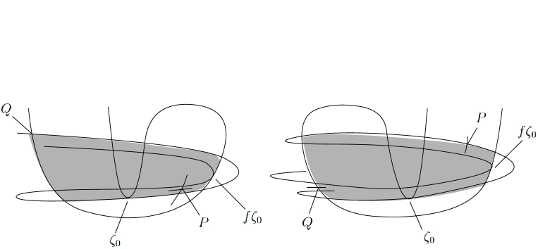
Figure 1. Manifold organization for $a=a^{*}$: orientation preserving/reversing cases (left/right). The shaded domains represent the rectangle $R$ (see Sect.2.2) containing the non wandering set $\Omega$.

We state our settings in more precise terms. Write $f$ for $f_{a^{*}}$. At a point $x\in\mathbb{R}^{2}$ define a one-dimensional subspace $E_{x}^{u}$ of $T_{x}\mathbb{R}^{2}$ which is exponentially contracted by backward iterates:

$$\limsup_{n\to\infty}\frac{1}{n}\log\|D_{x}f^{-n}|E^{u}_{x}\|<0.$$

Since $f^{-1}$ expands area, the one-dimensional subspace of $T_{x}\mathbb{R}^{2}$ with this property is unique, when it makes sense. We call $E^{u}_{x}$ an unstable direction at $x$, and define an unstable Jacobian at $x$ by $J^{u}(x)=\|D_{x}f|E^{u}_{x}\|.$ Let $\Omega$ denote the non wandering set of $f$, which is a compact set. By a result of [24], $E^{u}_{x}$ makes sense for any $x\in\Omega$, and $x\mapsto E_{x}^{u}$ is continuous on $\Omega$ except at $Q$ where it is merely measurable.

For $x\in\Omega$ define

$$\underline{\lambda}^{u}(x)=\liminf_{n\to\infty}\frac{1}{n}\sum_{i=0}^{n-1}\log J^{u}(f^{i}x)\ \text{ and }\ \bar{\lambda}^{u}(x)=\limsup_{n\to\infty}\frac{1}{n}\sum_{i=0}^{n-1}\log J^{u}(f^{i}x).$$

If both values coincide, then call this common value an unstable Lyapunov exponent at $x$ and denote it by $\lambda^{u}(x)$. Since the (non-uniform) expansion along the unstable direction is responsible for the chaotic behavior, the distribution of the unstable Lyapunov exponent is important for understanding the dynamics of $f$.

If $f$ preserves orientation, let $W^{u}=W^{u}(Q)$. Otherwise, let $W^{u}=W^{u}(P)$. A good deal of information is contained in the unstable slice

$$\Omega^{u}=\Omega\cap W^{u}.$$

For each $\beta\in\mathbb{R}$ consider the level set

$$\Omega^{u}(\beta)=\left\{x\in\Omega^{u}\colon\text{$\lambda^{u}(x)$ is defined and }\lambda^{u}(x)=\beta\right\}.$$

The first question to ask is what are the values of $\beta$ for which $\Omega^{u}(\beta)\neq\emptyset$. For uniformly hyperbolic systems as in the case $a>a^{*}$, such values are all positive and form a compact interval. One can easily see that this is not the case for $f=f_{a^{*}}$, because $\lambda^{u}(\zeta_{0})<0$.

Let $\mathcal{M}(f)$ denote the set of $f$-invariant Borel probability measures. An unstable Lyapunov exponent of a measure $\mu\in\mathcal{M}(f)$ is the number $\lambda^{u}(\mu)$ defined by

$$\lambda^{u}(\mu)=\int\log J^{u}d\mu.$$

Set

$$\lambda_{m}^{u}=\inf\{\lambda^{u}(\mu)\colon\mu\in\mathcal{M}(f)\}\ \text{ and }\ \lambda_{M}^{u}=\sup\{\lambda^{u}(\mu)\colon\mu\in\mathcal{M}(f)\}.$$

By a result of [6], $\lambda_{m}^{u}>0$. Since any measure is supported on the compact set $\Omega$, $\lambda_{M}^{u}<\infty$. Set $I=[\lambda_{m}^{u},\lambda_{M}^{u}].$

Theorem A.

Let $b>0$ be sufficiently small and $f=f_{a^{*}(b)}$ as above. Then $\Omega^{u}(\beta)\neq\emptyset$ if and only if $\beta\in\{\lambda^{u}(\zeta_{0})\}\cup I$.

The number $\lambda^{u}(\zeta_{0})$ equals the stable Lyapunov exponent of the Dirac measure at $Q$, and so $\lambda^{u}(\zeta_{0})\to-\infty$ as $b\to 0$. The interval $I$ does not degenerate to a point as $b\to 0$, because the unstable Lyapunov exponents of the Dirac measures at $P$ and $Q$ converge to $\log 2$ and $\log 4$ respectively. In fact, one can show that $\lambda_{m}^{u}\to\log 2$ and $\lambda_{M}^{u}\to\log 4$ as $b\to 0$.

A proof of Theorem A relies on the fact that $a^{*}\to 2$ as $b\to 0$, and so $f=f_{a^{*}}$ may be viewed as a singular perturbation of the endomorphism $(x,y)\mapsto(1-2x^{2},0)$. However, the multifractal picture is quite in contrast to that of the quadratic map $x\in[-1,1]\to 1-2x^{2}$. The Lyapunov exponent of the quadratic map takes only three values: it is $\log 4$ at the repelling fixed point $-1$ and its preimage $1$, $-\infty$ at the preimages of $0$, and is $\log 2$ at all other well-defined points.

Now, consider a multifractal decomposition

$$\Omega^{u}=\left(\bigcup_{\beta\in\{\lambda^{u}(\zeta_{0})\}\cup I}\Omega^{u}(\beta)\right)\cup\hat{\Omega}^{u},$$

where $\hat{\Omega}^{u}$ denotes the set of those $x\in\Omega^{u}$ for which $\underline{$\lambda$}^{u}(x)\neq\bar{\lambda}^{u}(x)$ and so $\lambda^{u}(x)$ is undefined. This decomposition has an extremely complicated topological structure. One can show that if $\beta\in I$, then $\Omega^{u}(\beta)$ is dense in $\Omega^{u}$ with respect to the induced topology on $W^{u}$.

To evaluate the size of each level set we adopt the Hausdorff dimension on $W^{u}$ defined as follows. Given $p\in(0,1]$ the unstable Hausdorff $p$-measure of a set $A\subset W^{u}$ is defined by

$$m_{p}^{u}(A)=\lim_{\varepsilon\to 0}\left(\inf\sum_{U\in\mathcal{U}}{\rm length}(U)^{p}\right),$$

where ${\rm length}(\cdot)$ denotes the length on $W^{u}$ with respect to the induced Riemannian metric, and the infimum is taken over all countable coverings $\mathcal{U}$ of $A$ by open sets of $W^{u}$ with length $\leq\varepsilon$. The unstable Hausdorff dimension of $A$, denoted by $\dim_{H}^{u}$, is the unique number in $[0,1]$ such that

$$\dim_{H}^{u}(A)=\sup\{p\colon m_{p}^{u}(A)=\infty\}=\inf\{p\colon m_{p}^{u}(A)=0\}.$$

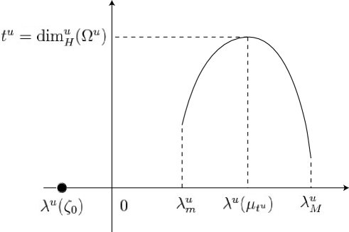
Figure 2. Schematic picture of the graph of the Lyapunov spectrum $L^{u}\colon\{\lambda^{u}(\zeta_{0})\}\cup I\to\mathbb{R}$.

Set

$$L^{u}(\beta)=\dim_{H}^{u}(\Omega^{u}(\beta)).$$

The object of our study is the function $\beta\mapsto L^{u}(\beta)$, called a Lyapunov spectrum.

We give a formula for $L^{u}(\beta)$ in terms of the unstable Lyapunov exponents and entropy of invariant probability measures. The entropy of $\mu\in\mathcal{M}(f)$ is denoted by $h(\mu)$.

Theorem B.

For any $\beta\in I$,

$$L^{u}(\beta)=\lim_{\varepsilon\to 0}{\sup}\left\{\frac{h(\mu)}{\lambda^{u}(\mu)}\colon\mu\in\mathcal{M}(f),\ \left|\lambda^{u}(\mu)-\beta\right|<\varepsilon\right\}.$$

Due to the existence of tangency, the unstable Lyapunov exponent as a function of measures may not be lower semi-continuous. Hence, the limit in $\varepsilon$ is necessary. A formula similar to the one in Theorem B was obtained in [8] for a positive measure set of quadratic maps $x\in[-1,1]\to 1-ax^{2}$, but only for the time averages of continuous functions.

We now move on to properties of the Lyapunov spectrum. Let us recall the thermodynamic formalism of $f$ developed in [24, 25]. For $t\in\mathbb{R}$ define

$$P(t)=\sup\left\{h(\mu)-t\lambda^{u}(\mu)\colon\mu\in\mathcal{M}(f)\right\}.$$

A measure which attains this supremum is called an equilibrium measure for $-t\log J^{u}$. The function $t\mapsto P(t)$ is convex. One has $P(0)>0$, and Ruelle’s inequality [23] gives $P(1)\leq 0$. Since $f$ has no SRB measure [28], $P(1)<0$ holds. Hence the equation $P(t)=0$ has a unique solution in $(0,1)$, denoted by $t^{u}$. There exists a unique equilibrium measure for $-t^{u}\log J^{u}$ ([25, Theorem A]), denoted by $\mu_{t^{u}}$, and $t^{u}=\dim_{H}^{u}(\Omega^{u})$, $t^{u}\to 1$ as $b\to 0$ ([25, Theorem B]).

Theorem C.

The following holds for the function $\beta\in I\mapsto L^{u}(\beta)$:

• it is continuous;

• increasing on $[\lambda_{m}^{u},\lambda^{u}(\mu_{t^{u}})]$ and decreasing on $[\lambda^{u}(\mu_{t^{u}}),\lambda_{M}^{u}]$;

• strictly positive in the interior of $I$;

• $L^{u}(\beta)=t^{u}$ if and only if $\beta=\lambda^{u}(\mu_{t^{u}})$.

Theorem C illustrates what is sometimes called a multifractal miracle. Even though the multifractal decomposition is topologically complicated, the Lyapunov spectrum which encodes the decomposition is continuous, and has several additional properties.

Remark. From Theorem C(b), the minimum of $L^{u}$ is attained at the boundary of $I$. It is not known if the minimum is strictly positive. Nor the convexity of the Lyapunov spectrum is known (See FIGURE 2 with care).

The last theorem states that $\hat{\Omega}^{u}$ carries a full Hausdorff dimension. For the subshift of finite type it is known [2] that the set of irregular points for which the time averages of a given continuous function do not converge carries the full dimension. Since $\log J^{u}$ is not continuous, the same argument does not work in our setting.

Theorem D.

$\dim_{H}^{u}(\hat{\Omega}^{u})=t^{u}.$

To handle the two-dimensional dynamics of $f$ without uniform hyperbolicity, a basic idea is to use a (locally defined) stable foliation to identify points on the same leaf (called long stable leaves in our terms, see Sect.2.8), and to recover the one-dimensional argument [7] as much as possible. Since the stable foliation is not globally defined, it is not possible to tell whether such a leaf through a given point exist. To bypass this difficulty we proceed in three steps:

• introduce critical points (Sect.2.4) in the spirit of Benedicks and Carleson [4];

• formulate a condition in terms of the speed of recurrence to the critical set, which is sufficient for the existence of the long stable leaf (Sect.2.7 and Sect.2.8):

• show that the unstable Lyapunov exponent does not exist at any point for which this condition fails (Sect.2.9).

The rest of this paper consists of two sections. In Sect.2 we collect mainly from [24, 25] and prove some results which will be needed later. In Sect.3 we bring them together and prove the theorems.

2. Preliminaries

In this section we collect from [24, 25] and prove some results which will be used in the proofs of the theorems.

2.1. Constants

Throughout this paper we shall be concerned with positive constants $\lambda$, $\delta$, $b$, the purposes of which are as follows:

• $\lambda$ is used to evaluate the rate of expansion of derivatives away from the point $\zeta_{0}$ of tangency (See Lemma 2.1);

• $\delta$ determines the size of a neighborhood of $\zeta_{0}$ (See Sect.2.3);

• $b$ determines the magnitude of the reminder term $b\cdot\Phi$ in (1).

The $\lambda$ is a fixed constant in $(0,\log 2)$. The $\delta$ and $b$ are small constants chosen in this order. The letter $C$ is used to denote any positive constant which is independent of $\delta$ or $b$.

2.2. The non wandering set

By a rectangle we mean any compact domain bordered by two compact curves in $W^{u}$ and two in the stable manifolds of $P$ or $Q$. By an unstable side of a rectangle we mean any of the two boundary curves in $W^{u}$. A stable side is defined similarly.

By the results of [24] there exists a rectangle $R$ contained in the set $\{(x,y)\in\mathbb{R}^{2}\colon|x|<2,|y|<\sqrt{b}\}$ with the following properties (See FIGURE 1):

• $\displaystyle{\Omega=\{x\in R\colon f^{n}x\in R\ \text{ for every }n\in\mathbb{Z}\}}$;

• one of the unstable sides of $R$ contains $\zeta_{0}$;

• one of the stable sides of $R$ contains $f\zeta_{0}$. This side is denoted by $\alpha_{0}^{+}$. The other side, denoted by $\alpha_{0}^{-}$, contains $Q$;

• $f\alpha_{0}^{+}\subset\alpha_{0}^{-}$.

2.3. Dynamics outside of critical region

Set

$$I(\delta)=\{(x,y)\in R\colon|x|<\delta\}.$$

Observe that $\zeta_{0}\in I(\delta)$. The next two lemmas state that the dynamics outside of $I(\delta)$ is “uniformly hyperbolic” and no critical behavior occurs. A slope $s(v)$ of a nonzero tangent vector $v=\left(\begin{smallmatrix}\xi\\ \eta\end{smallmatrix}\right)$ at a point in $\mathbb{R}^{2}$ is defined by $s(v)=|\eta|/|\xi|$ if $\xi\neq 0$, and $s(v)=\infty$ if $\xi=0$.

Lemma 2.1.

For any $\lambda\in(0,\log 2)$ and $\delta\in(0,1)$ there exists $b>0$ such that the following holds for $f=f_{a^{*}(b)}$: If $n\geq 1$ and $x\in R$ are such that $x,fx,\ldots,f^{n-1}x\notin I(\delta)$, then for any nonzero tangent vector $v$ at $x$ with $s(v)\leq\sqrt{b}$,

• $\|D_{x}f^{n}v\|\geq\delta e^{\lambda n}.$ If, in addition $f^{n}x\in I(\delta)$, then $\|D_{x}f^{n}v\|\geq e^{\lambda n}$;

• $s(D_{x}f^{n}v)\leq\sqrt{b}$.

Proof.

From the fact that $f$ may be viewed as a small perturbation of the map $x\mapsto 1-2x^{2}$. ∎

Lemma 2.2.

([27, Lemma 2.3]) Let $\gamma$ be a $C^{2}$ curve in $R$ and $x\in\gamma$. For each $i\geq 0$ let $\kappa_{i}(x)$ denote the curvature of $f^{i}\gamma$ at $f^{i}x$. Then

$$\kappa_{i}(x)\leq\frac{(Cb)^{i}}{\|D_{x}f^{i}|T_{x}\gamma\|^{3}}\kappa_{0}(x)+\sum_{j=1}^{i}\frac{(Cb)^{j}}{\|D_{f^{i-j}x}f^{j}|T_{f^{i-j}x}f^{i-j}\gamma\|^{3}}.$$

By a $C^{2}(b)$-curve we mean a compact, nearly horizontal $C^{2}$ curve in $R$ such that the slopes of its tangent directions are $\leq\sqrt{b}$ and the curvature is everywhere $\leq\sqrt{b}$.

Lemma 2.3.

If $\gamma$ is a $C^{2}(b)$-curve in $R$ not intersecting $I(\delta)$, then $f\gamma$ is a $C^{2}(b)$-curve.

Proof.

From Lemma 2.1 and Lemma 2.2. ∎

2.4. Critical points

Returns to the inside of $I(\delta)$ are inevitable and must be treated with care. A key ingredient is the notion of critical points, i.e., points of tangencies between $C^{2}(b)$-curves in $W^{u}$ and preimages of leaves of a stable foliation. We quote results from [24] surrounding critical points, and develop them slightly further.

From the hyperbolicity of the saddle $Q$, there exist two mutually disjoint connected open sets $U^{-}$, $U^{+}$ independent of $b$ such that $\alpha_{0}^{-}\subset U^{-}$, $\alpha_{0}^{+}\subset U^{+}$, $U^{+}\cap fU^{+}=\emptyset=U^{+}\cap fU^{-}$ and a foliation $\mathcal{F}^{s}$ of $U=U^{-}\cup U^{+}$ by one-dimensional leaves such that:

• $\mathcal{F}^{s}(Q)$, the leaf of $\mathcal{F}^{s}$ containing $Q$, contains $\alpha_{0}^{-}$;

• if $x,fx\in U$, then $f(\mathcal{F}^{s}(x))\subset\mathcal{F}^{s}(fx)$;

• Let $e^{s}(x)$ denote the unit vector in $T_{x}\mathcal{F}^{s}(x)$ whose second component is positive. Then $x\mapsto e^{s}(x)$ is $C^{1}$, $\|D_{x}fe^{s}(x)\|\leq Cb$ and $\|D_{x}e^{s}(x)\|\leq C$;

• If $x,fx\in U$, then $s(e^{s}(x))\geq C/\sqrt{b}.$

Definition 2.4.

We say $\zeta\in W^{u}\cap I(\delta)$ is a critical point if $f\zeta\in U^{+}$ and $T_{f\zeta}W^{u}=T_{f\zeta}\mathcal{F}^{s}(f\zeta)$.

From the first two conditions on $\mathcal{F}^{s}$ and $f\alpha_{0}^{+}\subset\alpha_{0}^{-}$, there is a leaf of $\mathcal{F}^{s}$ which contains $\alpha_{0}^{+}$. Since $f\zeta_{0}\in\alpha_{0}^{+}$ we have $f\zeta_{0}\in U^{+}$ and $T_{f\zeta_{0}}W^{u}=T_{f\zeta_{0}}\mathcal{F}^{s}(f\zeta_{0})$, namely, $\zeta_{0}$ is a critical point. The next lemma tells about the location of all other critical points. Let $S$ denote the compact lenticular domain bounded by the parabola $f^{-1}\alpha_{0}^{+}\cap R$ and the unstable side of $R$ not containing $\zeta_{0}$.

Lemma 2.5.

Let $\gamma$ be a $C^{2}(b)$-curve in $I(\delta)$ stretching across $I(\delta)$. Then there exists a unique critical point $\zeta\in\gamma$. In addition, $\zeta\in S$. if $\zeta\neq\zeta_{0}$ then $\zeta\in{\rm int}S$.

Proof.

We claim that any leaf of $\mathcal{F}^{s}$ at the right of the one containing $\alpha_{0}^{+}$ is tangent to $f\gamma$ and the tangency is quadratic, or else it intersects $f\gamma$ exactly at two points. This follows from [27, Lemma 2.2], the uniform boundedness of $\|D_{x}e^{s}(x)\|$ and $s(e^{s}(x))$. Hence there exists a critical point on $\gamma$. If $\zeta_{1}$, $\zeta_{2}$ are distinct critical points on $\gamma$, then the leaves $\mathcal{F}^{s}(f\zeta_{1})$, $\mathcal{F}^{s}(f\zeta_{1})$ must intersect each other, which is a contradiction. Hence the uniqueness holds. Since the quadratic tangency occurs on or at the right of $\alpha_{0}^{+}$, the last two statements hold. ∎

By Lemma 2.5, any critical point other than $\zeta_{0}$ is contained in the interior of $S$, so that it is mapped to the outside of $R$, and then escape to infinity under forward iteration. Hence, the critical orbits are contained in a region where the uniform hyperbolicity is apparent. By binding generic orbits which fall inside $I(\delta)$ to suitable critical points, and then copying the exponential growth along the critical orbits, one shows that the horizontal slopes and the expansion are restored after suffering from the loss due to the folding behavior near $I(\delta)$.

In the next lemma we assume $\delta>0$ is sufficiently small. Let $\zeta$ be a critical point and $x\in I(\delta)\setminus S$. We say a unit tangent vector $v$ at $x$ is in admissible position relative to $\zeta$ if there exists a $C^{2}(b)$-curve which is tangent to both $T_{\zeta}W^{u}$ and $v$. Set

(3) $$c(b)=-\frac{1}{\log b}.$$

Let us agree that for two positive real numbers $A$, $B$, $A\approx B$ indicates that both $A/B$, $B/A$ are bounded from above by a constant independent of $\delta$ or $b$.

Lemma 2.6.

Let $\zeta$ a critical point, $x\in(\Omega\cap I(\delta))\setminus S$ and $v$ be a unit tangent vector at $x$ in admissible position relative to $\zeta$. there exist positive integers $p=p(\zeta,x),q=(\zeta,x)$ such that:

• $q\leq-c(b)\log|\zeta-x|\ll-(2/3)\log|\zeta-x|\leq p$;

• $f^{i}\zeta$, $f^{i}x\in U$ for every $1\leq i\leq p$;

• $s(D_{x}f^{p}v)\leq\sqrt{b}$ and $\|D_{x}f^{p}v\|\geq e^{\frac{\lambda}{3}p}$;

• $\|D_{x}f^{q}v\|\leq C|\zeta-x|^{1-c(b)};$

• $\|D_{x}f^{i}v\|<1$ for every $1\leq i<q$ and $\|D_{x}f^{i}v\|\approx 2|\zeta-x|\cdot\|D_{fx}f^{i-1}\left(\begin{smallmatrix}1\\ 0\end{smallmatrix}\right)\|$ for every $q\leq i\leq p$.

Proof.

We only give a proof of (d). The rest of the items is contained in [24, Lemma 2.5]. Split $D_{x}fv=A\cdot\left(\begin{smallmatrix}1\\ 0\end{smallmatrix}\right)+B\cdot e^{s}(fx),$ $A$, $B\in\mathbb{R}$. Since the forward orbit of $f\zeta$ does not intersect $I(\delta)$, the tangent vector $\left(\begin{smallmatrix}1\\ 0\end{smallmatrix}\right)$ at $f\zeta$ grows exponentially in norm under forward iteration. Since the forward orbit of $fx$ shadows that of $f\zeta$, $\|D_{fx}f^{q-1}\left(\begin{smallmatrix}1\\ 0\end{smallmatrix}\right)\|\approx\|D_{f\zeta}f^{q-1}\left(\begin{smallmatrix}1\\ 0\end{smallmatrix}\right)\|$ holds. From the quadratic behavior near the critical point we have $|A|\approx|\zeta-x|$. Then, $q\ll p$ in Lemma 2.6(a) and the exponential contraction of $e^{s}(fx)$ implies $|A|\cdot\|D_{fx}f^{q-1}\left(\begin{smallmatrix}1\\ 0\end{smallmatrix}\right)\|\gg|B|\cdot\|D_{fx}f^{q-1}e^{s}(fx)\|$. Hence $\|D_{x}f^{q}v\|\approx|\zeta-x|\cdot\|D_{f\zeta}f^{q-1}\left(\begin{smallmatrix}1\\ 0\end{smallmatrix}\right)\|\leq C|\zeta-x|^{1-c(b)},$ where the last inequality follows from the definition of $q$ in [24, Sect.2.3]. ∎

2.5. Existence of binding points

We look for suitable critical points for returns to $I(\delta)$ with the help of the nice geometry of $W^{u}$ which is particular to the first bifurcation parameter $a^{*}$. Let $\alpha_{1}^{+}$ denote the connected component of $W^{s}(P)\cap R$ containing $P$, and $\alpha_{1}^{-}$ the connected component of $f^{-1}\alpha_{1}^{+}\cap R$ not containing $P$. Let $\Theta$ denote the rectangle bordered by $\alpha_{1}^{-}$, $\alpha_{1}^{+}$ and the unstable sides of $R$.

Lemma 2.7.

Let $\gamma$ be a $C^{2}(b)$-curve in $I(\delta)$ and suppose there exists a critical point on $\gamma$. If $n\geq 1$ is such that $\Theta\cap f^{i}\gamma=\emptyset$ for $i=0,1,\ldots,n-1$ and $f^{n}\gamma\cap\Theta\neq\emptyset$, then any connected component of $\Theta\cap f^{n}\gamma$ is a $C^{2}(b)$-curve.

Proof.

By Lemma 2.3 it suffices to show that for any $x\in\gamma$, $\|D_{f^{i}x}f^{n-i}|T_{f^{i}x}f^{i}\gamma\|\geq\delta$ for every $0\leq i\leq n-1$. This follows from Lemma 2.1 and Lemma 2.6(e). ∎

Let $\tilde{\Gamma}^{u}$ denote the collection of connected components of $\Theta\cap W^{u}$ with respect to the intrinsic topology on $W^{u}$.

Lemma 2.8.

Any element of $\tilde{\Gamma}^{u}$ is a $C^{2}(b)$-curve with endpoints in $\alpha_{1}^{-}$, $\alpha_{1}^{+}$.

Proof.

Let $\gamma$ denote the unstable side of $\Theta$ not containing $\zeta_{0}$. This is $C^{2}(b)$, and contains a fundamental domain in $W^{u}$. It suffices to show that for each $n\geq 0$, any connected component of $\Theta\cap\bigcup_{i=0}^{n}f^{i}\gamma$ is a $C^{2}(b)$-curve with endpoints in $\alpha_{1}^{-}$, $\alpha_{1}^{+}$. This holds for $n=0$. If it holds for $n=k$, then by Lemma 2.7, any connected component of $\Theta\cap\bigcup_{i=0}^{k+1}f^{i}\gamma$ is $C^{2}(b)$. Since the endpoints of $\gamma$ are mapped to the stable sides of $\Theta$, the statement holds for $n=k+1$. ∎

Define

$$\Gamma^{u}=\{\gamma^{u}\colon\text{$\gamma^{u}$ is the pointwise limit of the sequence in $\tilde{\Gamma}^{u}$}\}.$$

Since elements of $\tilde{\Gamma}^{u}$ are $C^{2}(b)$ by Lemma 2.8, the pointwise convergence is equivalent to the uniform convergence. Since curves in $\tilde{\Gamma}^{u}$ are pairwise disjoint, the uniform convergence is equivalent to the $C^{1}$ convergence. Hence, curves in $\Gamma^{u}$ are $C^{1}$ and the slopes of their tangent directions are $\leq\sqrt{b}$. Elements of $\Gamma^{u}$ are called long unstable leaves. Set

$$\mathcal{W}^{u}=\bigcup_{\gamma^{u}\in\Gamma^{u}}\gamma^{u}.$$

Figure 3. The long unstable leaves.

Several remarks are in order on the long unstable leaves:

• each leaf is the (strictly) monotone limit of curves in $\tilde{\Gamma}^{u}$, so that any connected component of $\mathcal{W}^{u}$ contains at most two leaves;

• two intersecting leaves are tangent at every point of the intersection;

• For $x\in\mathcal{W}^{u}$, $E_{x}^{u}=T_{x}\gamma^{u}$, where $\gamma^{u}$ denotes any leaf containing $x$ ([25, Lemma 3.2(P2)]);

• $\Omega\cap\Theta\subset\mathcal{W}^{u}$ ([24, Lemma 2.8]).

Lemma 2.9.

If $x\in\Omega\cap I(\delta)$, then there exists a critical point relative to which any unit vector spanning $E^{u}_{x}$ is in admissible position.

Proof.

A long stable leaf containing $x$ is accumulated in $C^{1}$ by curves in $\tilde{\Gamma}^{u}$, each of which contains a critical point by Lemma 2.5. ∎

If $x\in\Omega\cap I(\delta)$, then critical points as in Lemma 2.9 are not unique. Let $\zeta(x)$ denote the one which is closest to the saddle in $W^{u}$ with respect to the induced metric on $W^{u}$, and call it a binding point for $x$. Write $p(x)=p(\zeta(x),x)$, $q(x)=q(\zeta(x),x)$ and call them the fold and bound periods of $x$.

2.6. Bound-free structure

To the forward orbit of $x\in\Omega$ we associate a sequence

$$0\leq n_{1}<n_{1}+p_{1}<n_{2}<n_{2}+p_{2}<n_{3}<\cdots$$

of integers which record the pattern of recurrence to $I(\delta)$ in the following manner. First, $n_{1}=\min\{n\geq 0\colon f^{n}x\in I(\delta)\}$ and $p_{1}=p(f^{n_{1}}x)$. Given $n_{k}$ and $p_{k}$, set $n_{k+1}=\min\{n\geq n_{k}+p_{k}\colon f^{n}x\in I(\delta)\}$ and $p_{k+1}=p(f^{n_{k+1}}x)$. This decomposes the forward orbit of $x$ into segments corresponding to time intervals $(n_{k},n_{k}+p_{k})$ and $[n_{k}+p_{k},n_{k+1}]$, during which we refer to the points in the orbit of $x$ as being “bound” and “free” respectively. The $\{n_{k}\}_{k}$ are the only return times to $I(\delta)$.

2.7. Controlled points

For $x\in\Omega$ define

$$d_{\rm crit}(x)=\begin{cases}|\zeta(x)-x|&\text{ if $x\in I(\delta)$};\\ 1&\text{ otherwise,}\end{cases}$$

where $\zeta(x)$ is the binding point for $x$ determined in Sect.2.5.

Definition 2.10.

We say $x\in\Omega$ is controlled if $d_{\rm crit}(f^{n}x)>b^{\frac{n}{9}}$ holds for every $n\geq 0$.

The next lemma states that points without too deep returns to the criticality is controlled eventually.

Lemma 2.11.

Let $m\geq 0$. If $d_{\rm crit}(f^{n}x)>b^{\frac{n}{9}}$ for every $n\geq m$, then there exists $k\in[0,m]$ such that $f^{k}x$ is controlled.

Proof.

The statement for $m=0$ is immediate from the definition. Let $m=1$ and suppose that $f^{k}x$ is not controlled for every $k\in[0,m]$. Then, it is possible to define a sequence $\{k_{i}\}_{i=1}^{s}$ of nonnegative integers inductively as follows: $k_{1}=\min\{n\geq 0\colon d_{\rm crit}(f^{n}x)\leq b^{\frac{n}{9}}\}.$ Since $x\in G_{m}$ we have $k_{1}<m$. Given $k_{1},\ldots,k_{i}$ with $k_{1}+\cdots+k_{i}<m$ and $d_{\rm crit}(f^{k_{1}+\cdots+k_{i}}x)\leq b^{\frac{k_{i}}{9}}$, define $k_{i+1}=\min\{n>0\colon d_{\rm crit}(f^{k_{1}+\cdots+k_{i}+n}x)\leq b^{\frac{n}{9}}\}.$ We have $k_{1}+\cdots+k_{s-1}<m\leq k_{1}+\cdots+k_{s}$. Since $b^{\frac{k_{i}}{9}}\cdot\|Df^{2k_{i}}\|\ll 1$, $f^{k_{1}+\cdots+k_{i}}x$ shadows the forward orbit of the binding point at least up to time $2k_{i}$, and so $2k_{i}<k_{i+1}$. This yields $k_{1}+\cdots+k_{s}<2k_{s}$, and thus $d_{\rm crit}(f^{k_{1}+\cdots+k_{s}}x)\leq b^{\frac{k_{s}}{9}}<b^{\frac{2(k_{1}+\cdots+k_{s})}{9}}.$ From the assumption on $x$ and $m\leq k_{1}+\cdots+k_{s}$ we have $d_{\rm crit}(f^{k_{1}+\cdots+k_{s}}x)>b^{\frac{k_{1}+\cdots+k_{s}}{9}}.$ These two inequalities yield a contradiction. ∎

2.8. Long stable leaves

By a vertical $C^{2}(b)$-curve we mean a compact, nearly vertical $C^{2}$ curve in $R$ with endpoints in the unstable sides of $R$, and of the form

$$\{(x(y),y)\colon|x^{\prime}(y)|\leq C\sqrt{b},|x^{\prime\prime}(y)|\leq C\sqrt{b}\}.$$

A vertical $C^{2}(b)$-curve $\gamma^{s}$ is called a long stable leaf if for any $x,y\in\gamma^{s}$, $|f^{n}x-f^{n}y|\leq Cb^{\frac{n}{2}}$ holds for every $n\geq 0$.

Lemma 2.12.

If $x\in\Omega$ is controlled, then there exists a unique long stable leaf through $x$, denoted by $\gamma^{s}(x)$. In addition, the following holds:

• for all $y$, $z\in\gamma^{s}(x)\cap\Omega$ and $n>0$,

  $$\frac{\|D_{y}f^{n}|E_{y}^{u}\|}{\|D_{z}f^{n}|E_{z}^{u}\|}\leq 2;$$

• if $x,y\in\Omega$ are controlled, then the Hausdorff distance between $\gamma^{s}(x)$ and $\gamma^{s}(y)$ is $\leq e^{C\sqrt{b}}|x-y|$.

Proof.

In view of the results in [17, Sect.6, Sect.7C], [5, Lemma 2.4] [25, Sublemma A.2], it suffices to show the following expansion estimate:

(4) $$\|D_{x}f^{n}|E^{u}_{x}\|\geq b^{\frac{n}{10}}\text{ for every $n\geq 1$.}$$

To show (4) we introduce the bound/free structure on the orbit of $x$. If $f^{n}x$ is free, then the orbit $x,\ldots,f^{n}x$ is decomposed into alternate bound and free segments. Applying the expansion estimates in Lemma 2.1 and Lemma 2.6 we have $\|D_{x}f^{n}|E^{u}_{x}\|\geq\delta e^{\frac{\lambda}{3}n}>b^{\frac{n}{10}}$. If $f^{n}x$ is bound, then there exists an integer $0<m<n$ such that $f^{m}x\in I(\delta)$ and $m<n<m+p$, where $p$ is the bound period of $f^{m}x$. Since $f^{m+p}x$ is free and $\|Df\|<5$ we have $\|D_{x}f^{n}|E^{u}_{x}\|\geq 5^{-(m+p-n)}\|D_{x}f^{m+p}|E^{u}_{x}\|>5^{-p}$. Since $x$ is controlled, $p\leq-(2n/27)\log b$ and so $\|D_{x}f^{n}|E^{u}_{x}\|\geq b^{\frac{2\log 5}{27}n}.$ ∎

2.9. Points with too deep returns are negligible

For each $m\geq 0$ define

$$G_{m}=\{x\in\Omega\colon\text{$d_{\rm crit}(f^{n}x)>b^{\frac{n}{10}}$ for every $n\geq m$}\}.$$

Set

$$\Omega_{*}=\Omega\setminus\bigcup_{m=0}^{\infty}G_{m}.$$

This is the set of points which return to the deep inside of the criticality. It is true that we lose control of derivatives on $\Omega_{*}$. However, the next lemma states that unstable Lyapunov exponents are undefined on $\Omega_{*}$. Hence, we may neglect $\Omega_{*}$ for our purpose.

Lemma 2.13.

If $x\in\Omega_{*}$, then $\underline{\lambda}^{u}(x)\neq\bar{\lambda}^{u}(x)$.

Proof.

Consider the bound/free structure in Sect.2.6 for the forward orbit of $x$. By definition, $d_{\rm crit}(f^{n}x)\leq b^{\frac{n}{10}}$ holds for infinitely many $n>0$. For these $n$, $f^{n}x$ is free. By Lemma 2.6 and (3), the corresponding fold period $q=q(f^{n}x)$ satisfies

$$q\leq-c(b)d_{\rm crit}(f^{n}x)\leq-c(b)\frac{n}{10}\log b=\frac{n}{10}.$$

Hence $n+q\leq(11/10)n$, and by Lemma 2.6(c),

$$\|D_{f^{n}x}f^{q}|E^{u}_{f^{n}x}\|\leq Cd_{\rm crit}(f^{n}x)^{1-c(b)}\leq Cb^{\frac{(1-c(b))}{10}n}\leq Cb^{\frac{(1-c(b))10}{11}(n+q)}.$$

Hence we have

$$\|D_{x}f^{n+q}|E^{u}_{x}\|=\|D_{x}f^{n}|E^{u}_{x}\|\cdot\|D_{f^{n}x}f^{q}|E^{u}_{f^{n}x}\|<5^{n}\cdot Cb^{\frac{(1-c(b))10}{11}(n+q)}<b^{\frac{n+q}{2}}.$$

Since this holds for infinitely many $n>0$, we obtain $\underline{\lambda}^{u}(x)\leq(1/2)\log b<0$. On the other hand, decomposing the forward orbit of $x$ into alternate bound and free segments, and then applying the expansion estimates in Lemma 2.1 and Lemma 2.6 imply $\bar{\lambda}^{u}(x)\geq\lambda/3>0.$ ∎

Corollary 2.14.

For any $\mu\in\mathcal{M}(f)$, $\mu(\Omega_{*})=0$.

Proof.

From the ergodic decomposition, it suffices to consider the case where $\mu$ is ergodic. From the Ergodic Theorem, $\underline{\lambda}^{u}(x)=\bar{\lambda}^{u}(x)$ holds for $\mu$-a.e. $x$. Hence $\mu(\Omega_{*})=0$. ∎

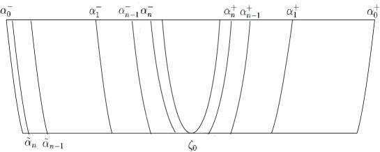
Figure 4. The rectangle $R$ and the curves $\{\tilde{\alpha}_{n}\}$, $\{\alpha_{n}^{+}\}$, $\{\alpha_{n}^{-}\}$. The $\{\tilde{\alpha}_{n}\}$ accumulate on the left stable side of $R$. Both $\{\alpha_{n}^{+}\}$ and $\{\alpha_{n}^{-}\}$ accumulate on the parabola $f^{-1}\alpha_{0}^{+}\cap R$ containing the point of tangency $\zeta_{0}$ near the origin.

2.10. Inducing

We now recall the inducing construction performed in [25]. Define a sequence $\{\tilde{\alpha}_{n}\}_{n=0}^{\infty}$ of compact curves in $W^{s}(P)\cap R$ inductively as follows. First, set $\tilde{\alpha}_{0}=\alpha_{1}^{+}$. Given $\tilde{\alpha}_{n-1}$, define $\tilde{\alpha}_{n}$ to be one of the two connected components of $R\cap f^{-1}\tilde{\alpha}_{n-1}$ which is at the left of $\zeta_{0}$. Observe that $\tilde{\alpha}_{1}=\alpha_{1}^{-}$. By the Inclination Lemma, the Hausdorff distance between $\tilde{\alpha}_{n}$ and $\alpha_{0}^{-}$ converges to $0$ as $n\to\infty$.

For each $n\geq 0$ let $\alpha_{n}$ denote the connected component of $R\cap f^{-1}\tilde{\alpha}_{n}$ which is not $\tilde{\alpha}_{n+1}$. The set $R\cap f^{-1}\alpha_{n}$ consists of two curves, one at the left of $\zeta_{0}$ and the other at the right. They are denoted by $\alpha_{n+1}^{-}$, $\alpha_{n+1}^{+}$ respectively. By definition, these curves obey the following diagram

$$\{\alpha_{n+1}^{-},\alpha_{n+1}^{+}\}\stackrel{{\scriptstyle f^{2}}}{{\to}}\tilde{\alpha}_{n}\stackrel{{\scriptstyle f}}{{\to}}\tilde{\alpha}_{n-1}\stackrel{{\scriptstyle f}}{{\to}}\tilde{\alpha}_{n-2}\stackrel{{\scriptstyle f}}{{\to}}\cdots\stackrel{{\scriptstyle f}}{{\to}}\tilde{\alpha}_{1}=\alpha_{1}^{-}\stackrel{{\scriptstyle f}}{{\to}}\tilde{\alpha}_{0}=\alpha_{1}^{+}.$$

Define $r\colon\Theta\to\mathbb{N}\cup\{\infty\}$ by

$$r(x)=\inf(\{n>0\colon f^{n}x\in\Theta\}\cup\{\infty\}),$$

which is the first return time of $x$ to $\Theta$. Note that:

• $r(x)=1$ if and only if $x\in\alpha_{1}^{-}\cup\alpha_{1}^{+}$; $r(x)=n+1$ $(n\geq 1)$ if and only if $x$ is sandwiched by $\alpha_{n}^{+}$ and $\alpha_{n+1}^{+}$, or by $\alpha_{n}^{-}$ and $\alpha_{n+1}^{-}$; $r(x)=\infty$ if and only if $x\in S$;

• each level set of $r$ except $S$ has exactly two connected components.

Let $\mathcal{P}$ denote the partition of the set $\Theta\setminus(S\cup\alpha_{1}^{-}\cup\alpha_{1}^{+})$ into connected components of the level sets of the function $r$. The $\mathcal{P}$ is well-defined because $\alpha_{n}$ and $\alpha_{0}^{+}$ are long stable leaves, and the Hausdorff distance between them converges to $0$ as $n\to\infty$ by Lemma 2.12(b). Set $\mathcal{P}_{1}=\{\omega=\overline{\eta}\colon\eta\in\mathcal{P}\}$, where the bar denotes the closure operation. For each $n\geq 2$ define

$$\mathcal{P}_{n}=\left\{\omega_{0}\cap\bigcap_{i=1}^{n-1}f^{-r(\omega_{0})}\circ f^{-r(\omega_{1})}\circ\cdots\circ f^{-r(\omega_{i-1})}\omega_{i}\colon\omega_{0},\omega_{1},\ldots,\omega_{n-1}\in\mathcal{P}_{1}\right\}.$$

Elements of $\bigcup_{n\geq 0}\mathcal{P}_{n}$ are called proper rectangles. It is easy to see the following holds:

• the unstable sides of a proper rectangle are formed by two curves contained in the unstable sides of $\Theta$. Its stable sides are formed by two curves contained in $W^{s}(P)$;

• two proper rectangles are either nested, disjoint, or intersect each other only at their common stable sides.

On the interior of each $\omega\in\mathcal{P}_{1}$, the value of $r$ is constant. This value is denoted by $r(\omega)$. For each $\omega\in\mathcal{P}_{n}$ define its inducing time $\tau(\omega)$ by

(5) $$\tau(\omega)=\sum_{i=0}^{n-1}r(\omega_{i}).$$

It is easy to see the following holds:

• the unstable sides of $f^{\tau(\omega)}\omega$ are formed by two curves in $\tilde{\Gamma}^{u}$. Its stable sides are formed by two curves contained in the stable sides of $\Theta$ (See FIGURE 5);

• let $k\in(0,\tau(\omega))$. Then ${\rm int}\Theta\cap f^{k}\omega\neq\emptyset$ if and only if $k=r(\omega_{0})+\cdots+r(\omega_{i})$ for some $i\in[0,n-1]$.

Lemma 2.15.

For any $\gamma^{u}\in\Gamma^{u}$ and any proper rectangle $\omega$, $\gamma^{u}\cap\omega$ is a compact curve joining the stable sides of $\omega$. In addition,

• $\displaystyle{\sup_{x\in\gamma^{u}\cap\omega}\|D_{x}f^{\tau(\omega)}|E_{x}^{u}\|\geq e^{\frac{\lambda}{3}\tau(\omega)}};$

• $\displaystyle{\sup_{x,y\in\gamma^{u}\cap\omega}\frac{\|D_{y}f^{\tau(\omega)}|E_{y}^{u}\|}{\|D_{x}f^{\tau(\omega)}|E_{x}^{u}\|}\leq C|f^{\tau(\omega)}x-f^{\tau(\omega)}y|}.$

Proof.

From the first property of the proper rectangles and Lemma 2.8, any curve in $\tilde{\Gamma}^{u}$ intersects any of the stable sides of $\omega$ exactly at one point, and this intersection is transverse. Since $\gamma^{u}$ is a $C^{1}$-limit of curves in $\tilde{\Gamma}^{u}$, The first assertion follows. For (a) (b), see [25, Lemma 3.5]. ∎

Lemma 2.16.

The following holds for each $\omega\in\mathcal{P}_{n}$:

• $\tau(\omega)\geq 2n$;

• let $\partial^{u}\omega$ denote any unstable side of $\omega$. Then ${\rm length}(\partial^{u}\omega)\leq e^{-\lambda n}$;

• if $x\in\omega$, then $d_{\rm crit}(f^{n}x)\geq e^{-10\tau(\omega)}$ for every $0\leq n\leq\tau(\omega)-1.$

Proof.

(a) follows from (5) and $\min\{r(\omega)\colon\omega\in\mathcal{P}_{1}\}=2$. (b) follows from (a) and the fact that $f^{\tau(\omega)}$ maps $\partial^{u}\omega$ with uniform expansion as in Lemma 2.15 to a curve in $\tilde{\Gamma}^{u}$ of length nearly $1$. If (c) is not the case, then $f^{\tau(\omega)}x$ is still close to $Q$, a contradiction. ∎

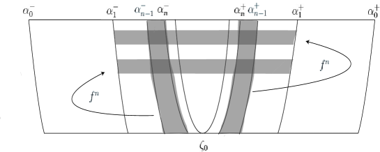
Figure 5. The proper rectangles (shaded) in $\mathcal{P}_{1}$ with inducing time $n$ and their $f^{n}$-images

2.11. Rectangles containing points without too deep returns

We need two lemmas on the recurrence properties of proper rectangles intersecting $G_{m}$.

Lemma 2.17.

Let $\omega$ be a proper rectangle such that $\omega\cap G_{m}\neq\emptyset$ for some $m\geq 0$. If $\tau(\omega)>m$, then for any $x\in\omega$,

$$d_{\rm crit}(f^{n}x)>b^{\frac{n}{9}}\ \text{ for every }\ m\leq n\leq\tau(\omega)-1.$$

Proof.

Let $m\leq n\leq\tau(\omega)-1$ be such that $f^{n}\omega\cap I(\delta)\neq\emptyset$. Choose $x_{0}\in\omega\cap G_{m}$. The $f^{n+1}\omega$ is contained in a rectangle whose stable sides are two neighboring curves in $\{\alpha_{k}\}_{k>0}$. From the quadratic behavior near the critical points and the exponential convergence of the curves $\{\alpha_{k}\}_{k>0}$ to $\alpha_{0}$ with exponent $\log 4$, for any $x\in\omega$ we have $2d_{\rm crit}(f^{n}x)^{2}>(1/16)2d_{\rm crit}(f^{n}x_{0})^{2}$. This yields $d_{\rm crit}(f^{n}x)>(1/4)d_{\rm crit}(f^{n}x_{0})\geq(1/4)b^{\frac{n}{10}}>b^{\frac{n}{9}}$. ∎

Lemma 2.18.

Let $\omega$ be a proper rectangle such that $\omega\cap G_{m}\neq\emptyset$ for some $m\geq 0$. If $\tau(\omega)>m$, then there exists $k\in[0,m]$ such that the stable sides of $f^{k}\omega$ are contained in long stable leaves.

Proof.

Let $\partial^{s}\omega$ denote any stable side of $\omega$ and $z$ an endpoint of $\partial^{s}\omega$. By Lemma 2.12 and Lemma 2.11, it suffices to show $d_{\rm crit}(f^{n}z)>b^{\frac{n}{9}}$ for every $n\geq m.$ Since $\omega\cap G_{m}\neq\emptyset$, this for $m\leq n\leq\tau(\omega)-1$ follows from Lemma 2.17. Since $f^{\tau(\omega)}z\in\alpha_{1}^{-}\cup\alpha_{1}^{+}$, for every $n\geq\tau(\omega)$ we have $f^{n}z\in f^{n-\tau(\omega)}(\alpha_{1}^{-}\cup\alpha_{1}^{+})\subset\alpha_{1}^{+}$, and so the desired inequality for every $n\geq\tau(\omega)$. ∎

2.12. Symbolic dynamics

Let $\mathcal{A}$ be a finite collection of proper rectangles contained in the interior of $\Theta$, labeled with $1,2,\ldots,\ell=\#\mathcal{A}$. We assume any two elements of $\mathcal{A}$ are either disjoint, or intersect each other only at their stable sides. Endow $\Sigma_{\ell}=\{1,\ldots,\ell\}^{\mathbb{Z}}$ with the product topology of the discrete topology, and let $\sigma\colon\Sigma_{\ell}\circlearrowleft$ denote the left shift. Define a coding map $\pi\colon\Sigma_{\ell}\to\mathbb{R}^{2}$ by $\pi(\{x_{i}\}_{i\in\mathbb{Z}})=y$, where

$$\{y\}=\left(\bigcap_{k=1}^{\infty}\omega_{k}^{s}\right)\cap\left(\bigcap_{k=1}^{\infty}\omega_{k}^{u}\right)$$

and

$$\omega^{s}_{k}=\omega_{x_{0}}\cap\left(\bigcap_{i=1}^{k}f^{-\tau(\omega_{x_{0}})}\circ\cdots\circ f^{-\tau(\omega_{x_{i-1}})}\omega_{x_{i}}\right)\text{ and }\omega^{u}_{k}=\bigcap_{i=1}^{k}f^{\tau(\omega_{x_{-1}})}\circ\cdots\circ f^{\tau(\omega_{x_{-i}})}\omega_{x_{-i}}.$$

Lemma 2.19.

The map $\pi$ is well-defined, continuous, injective, and satisfies $\pi(\Sigma_{\ell})\subset\Omega$.

Proof.

To show that $\left(\bigcap_{k=1}^{\infty}\omega_{k}^{s}\right)\cap\left(\bigcap_{k=1}^{\infty}\omega_{k}^{u}\right)$ is a singleton and so $\pi_{\mathcal{A}}$ is well-defined, it suffices to show that both $\omega^{s}_{k}$ and $\omega^{u}_{k}$ get thinner as $k$ increases, and converge to curves intersecting each other exactly at one point. We argue as follows.

Since $\#\mathcal{A}$ is finite, the elements of $\mathcal{A}$ do not accumulate the parabola $f^{-1}\alpha_{0}^{+}\cap R$. By Lemma 2.18 there exists $k_{0}\geq 1$ such that for each $k\geq k_{0}$, the stable sides of $F\omega^{s}_{k}$ are contained in long stable leaves, where $F=f^{\tau(\omega_{x_{0}})+\cdots+\tau(\omega_{x_{k_{0}}})+1}$. By the exponential decrease of the lengths of the unstable sides of this rectangle in $k$, and by Lemma 2.12(b), these long stable leaves converge as $k\to\infty$ to a single long stable leaf, denoted by $\gamma^{s}$. It follows that $\bigcap_{k=1}^{\infty}\omega^{s}_{k}$ is a curve contained in $F^{-1}\gamma^{s}$, joining the two unstable sides of $R$.

The unstable sides of $\omega_{k}^{u}$ belong to $\tilde{\Gamma}^{u}$. By [24, Lemma 2.2], the Hausdorff distance between them decreases exponentially in $k$. This implies $\bigcap_{k=1}^{\infty}\omega_{k}^{u}\in\Gamma^{u}$. Hence $\left(\bigcap_{k=1}^{\infty}\omega_{k}^{s}\right)\cap\left(\bigcap_{k=1}^{\infty}\omega_{k}^{u}\right)\neq\emptyset$ holds.

We have

$$F\left(\left(\bigcap_{k=1}^{\infty}\omega_{k}^{s}\right)\cap\left(\bigcap_{k=1}^{\infty}\omega_{k}^{u}\right)\right)\subset F\left(\bigcap_{k=1}^{\infty}\omega_{k}^{s}\right)\cap F\left(\omega_{k_{0}}^{s}\cap\bigcap_{k=1}^{\infty}\omega_{k}^{u}\right).$$

The first set of the right-hand-side is a subset of $\gamma^{s}$ and the second is in $\Gamma^{u}$. Hence, the set of the left-hand-side is a singleton. Since $F$ is a diffeomorphism, $\left(\bigcap_{k=1}^{\infty}\omega_{k}^{s}\right)\cap\left(\bigcap_{k=1}^{\infty}\omega_{k}^{u}\right)$ is a singleton.

Since all points outside of $R$ diverges to infinity under positive or negative iteration, we have $y\in\bigcap_{n\in\mathbb{Z}}f^{n}R$, and so $y\in\Omega$ from the first property of the rectangle $R$ in Sect.2.2. In addition, the above argument shows the continuity of $\pi$.

To show the injectivity, assume $x,y\in\Sigma_{\ell}$, $x\neq y$ and $\pi(x)=\pi(y)$. Then $\pi(x)$ is contained in the stable side of two neighboring elements of $\mathcal{A}$. Hence $f^{n}\pi(x)$ is not contained in the interior of $\Theta$ for every $n\geq 1$, a contradiction. ∎

2.13. Bounded distortion

We establish distortion bounds for proper rectangles.

Lemma 2.20.

For every $m\geq 0$ there exists a constant $D_{m}>0$ such that for any proper rectangle $\omega$ intersecting $G_{m}$ and $\tau(\omega)>m$,

$$\sup_{x,y\in\Omega\cap\omega}\frac{\|D_{y}f^{\tau(\omega)}|E_{y}^{u}\|}{\|D_{x}f^{\tau(\omega)}|E_{x}^{u}\|}\leq D_{m}.$$

Proof.

Let $x,y\in\Omega\cap\omega$. By the last remark on long unstable leaves in Sect.2.5, $\Omega\cap\omega\subset\mathcal{W}^{u}$. Take a stable side of $\omega$ and denote it by $\partial^{s}\omega$. Take $x^{\prime}\in\partial^{s}\omega$ (resp. $y^{\prime}\in\partial^{s}\omega$) such that $x$ and $x^{\prime}$ (resp. $y$ and $y^{\prime}$) lie on the same long unstable leaf. The Chain Rule gives

$$\frac{\|D_{y}f^{\tau(\omega)}|E_{y}^{u}\|}{\|D_{x}f^{\tau(\omega)}|E_{x}^{u}\|}=\frac{\|D_{x^{\prime}}f^{\tau(\omega)}|E_{x^{\prime}}^{u}\|}{\|D_{x}f^{\tau(\omega)}|E_{x}^{u}\|}\cdot\frac{\|D_{y^{\prime}}f^{\tau(\omega)}|E_{y^{\prime}}^{u}\|}{\|D_{x^{\prime}}f^{\tau(\omega)}|E_{x^{\prime}}^{u}\|}\cdot\frac{\|D_{y}f^{\tau(\omega)}|E_{y}^{u}\|}{\|D_{y^{\prime}}f^{\tau(\omega)}|E_{y^{\prime}}^{u}\|}.$$

Lemma 2.15(b) bounds the first and the third factors. For the second one, by Lemma 2.18 there exists $k\in[0,m]$ such that $f^{k}\partial^{s}\omega$ is contained in a long stable leaf. Then

$$\frac{\|D_{y^{\prime}}f^{\tau(\omega)}|E_{y^{\prime}}^{u}\|}{\|D_{x^{\prime}}f^{\tau(\omega)}|E_{x^{\prime}}^{u}\|}\leq\frac{\|D_{y^{\prime}}f^{k}|E_{y^{\prime}}^{u}\|}{\|D_{x^{\prime}}f^{k}|E_{x^{\prime}}^{u}\|}+\frac{\|D_{f^{k}y^{\prime}}f^{\tau(\omega)-k}|E_{f^{k}y^{\prime}}^{u}\|}{\|D_{f^{k}x^{\prime}}f^{\tau(\omega)-k}|E_{f^{k}x^{\prime}}^{u}\|}.$$

The first term of the right-hand-side is bounded by a uniform constant which depends only on $m$ and $f$. The second one is bounded by Lemma 2.12(a). ∎

2.14. Approximation of ergodic measures with horseshoes

Katok established the remarkable result that every hyperbolic measures of differomorphisms can be in a particular sense approximated by uniformly hyperbolic horseshoes (See [16, Theorem S.5.9] for the precise statement). We will need a version of this. Let $\mathcal{M}^{e}(f)$ denote the set of $f$-invariant ergodic Borel probability measures.

Lemma 2.21.

Let $\mu\in\mathcal{M}^{e}(f)$ satisfy $h(\mu)>0$. For any $\varepsilon>0$ there exist $q>0$ and a finite collection $\mathcal{R}$ of proper rectangles such that:

• for each $\omega\in\mathcal{R}$, $\tau(\omega)=q$;

• $\left|(1/q)\log\#\mathcal{R}-h(\mu)\right|<\varepsilon;$

• for any $x\in\bigcup_{\omega\in\mathcal{R}}\mathcal{W}^{u}\cap\omega$, $\left|(1/q)\sum_{i=0}^{q-1}\log J^{u}(f^{i}x)-\lambda^{u}(\mu)\right|<\varepsilon$.

Proof.

By [16, Theorem S.5.9], for any $\varepsilon\in(0,2h(\mu))$ there exists $\nu\in\mathcal{M}^{e}(f)$ which is supported on a hyperbolic set and satisfies $|h(\mu)-h(\nu)|<\varepsilon/2$, $|\lambda^{u}(\mu)-\lambda^{u}(\nu)|<\varepsilon/3$. We have $\nu(\Theta)>0$, for otherwise $\nu$ the Dirac measure at $Q$, in contradiction to $h(\nu)>0$.

Let $\omega_{\rm S}$ (resp. $\omega_{\rm R}$) denote the connected component of $R\setminus\Theta$ at the left (resp. right) of $\zeta_{0}$, and define

$$\mathcal{Q}(\nu)=\{\omega\in\mathcal{P}_{1}\colon\nu(\omega)>0\}\bigcup\{\omega_{\rm S},\omega_{\rm R}\}.$$

Since $\nu$ is supported on a hyperbolic set, $\#\mathcal{Q}(\nu)$ is finite. We claim that $\mathcal{Q}(\nu)$ is a generating partition with respect to $\nu$. Indeed, by [24, Lemma 3.1], there is a continuous surjection $\iota$ from $\Sigma_{2}$ to $\Omega$ which gives a symbolic coding of points in $\Omega$. Since the coding is given by the two rectangles intersecting only at $\zeta_{0}$, for any cylinder set $A$ in $\Sigma_{2}$, $\iota(A)\cap\bigcup\{\omega\colon\omega\in\mathcal{Q}(\nu)\}$ belongs to the sigma-algebra generated by $\bigcup_{n=0}^{\infty}\bigvee_{i=-n}^{n}f^{-i}\mathcal{Q}(\nu)$. Since cylinder sets form a base of the topology of $\Sigma_{2}$, the claim holds.

For $m>0$ let $\Lambda_{m}$ denote the set of all $x\in\Theta$ for which the following holds:

• $|(1/n)\log\nu(\omega(x))+h(\nu)|<\varepsilon/3$ for every $n\geq m$, where $\omega(x)$ denotes the element of $\bigvee_{i=0}^{n-1}f^{-i}\mathcal{Q}(\nu)$ containing $x$;

• $\left|(1/n)\sum_{i=0}^{n-1}\log J^{u}(f^{i}x)-\lambda^{u}(\nu)\right|\leq\varepsilon/3$ for every $n\geq m$;

• $x\in G_{m}$.

By the Shannon-McMillan-Breimann Theorem, the Ergodic Theorem and Corollary 2.14, $\nu(\Lambda_{m})\to\nu(\Theta)$ as $m\to\infty$. Let

$$\Lambda_{m,p}=\{x\in\Lambda_{m}\colon f^{q}x\in\Theta\text{ for some }q\in[p,2p]\}.$$

We claim $\nu(\Lambda_{m,p})\to\nu(\Lambda_{m})$ as $p\to\infty$. To show this, denote by $\chi_{\Theta}$ the characteristic function of $\Theta$. Set

$$B_{p}=\left\{x\in\Lambda_{m}\colon\frac{1}{p}\sum_{i=0}^{p-1}\chi_{\Theta}(f^{i}x)<\frac{5}{4}\nu(\Theta)\text{ and }\frac{1}{2p}\sum_{i=0}^{2p-1}\chi_{\Theta}(f^{i}x)>\frac{5}{8}\nu(\Theta)\right\}.$$

From the Ergodic Theorem, $\nu(B_{p})\to\nu(\Lambda_{m})$ as $p\to\infty$. Since $B_{p}\subset\Lambda_{m,p}$ the claim holds.

Choose $m>0$ such that $\nu(\Lambda_{m})\geq(1/2)\nu(\Theta)$, and then choose $p\geq m$ such that $\nu(\Lambda_{m,p})\geq(1/3)\nu(\Theta)$, $-(1/p)\log(6p)+(1/p)\log\nu(\Theta)>-\varepsilon/6$ and $D_{m}/p<\varepsilon/3$, where $D_{m}$ is the constant in Lemma 2.20. For each $q\in[p,2p]$ set

$$\Lambda_{m,p,q}=\{x\in\Lambda_{m,p}\colon\min\{n\in[p,2p]\colon f^{n}x\in\Theta\}=q\}.$$

Choose $q$ such that $\nu(\Lambda_{m,p,q})\geq(1/2p)\nu(\Lambda_{m,p})$. Define $\mathcal{R}$ to be the collection of proper rectangles intersecting $\Lambda_{m,p,q}$ with inducing time $q$. Lemma 2.21(a) is immediate from the construction.

Note that elements of $\mathcal{R}$ are mutually disjoint, altogether cover $\Lambda_{m,p,q}$ and belong to $\bigvee_{i=0}^{q-1}f^{-i}\mathcal{Q}(\nu)$. (i) gives $\nu(\omega)\leq e^{-q\left(h(\nu)-\frac{\varepsilon}{3}\right)}$ for each $\omega\in\mathcal{R}$. Hence

$$\#\mathcal{R}\geq\nu(\Lambda_{m,p,q})e^{q\left((h(\nu)-\frac{\varepsilon}{3}\right)}\geq\frac{1}{6p}\nu(\Theta)e^{q\left((h(\nu)-\frac{\varepsilon}{3}\right)},$$

and therefore

$$\frac{1}{q}\log\#\mathcal{R}\geq-\frac{1}{q}\log(6p)+\frac{1}{q}\log\nu(\Theta)+h(\nu)-\frac{\varepsilon}{3}>h(\nu)-\frac{\varepsilon}{2}>h(\mu)-\varepsilon.$$

Similarly we obtain $(1/q)\log\#\mathcal{R}\leq h(\nu)+\varepsilon/3$. This proves Lemma 2.21(b).

For each $\omega\in\mathcal{R}$ choose $x_{\omega}\in\omega\cap\Lambda_{m,p,q}$ such that $\left|(1/q)\sum_{i=0}^{q-1}\log J^{u}(f^{i}x_{\omega})-\lambda^{u}(\nu)\right|<\varepsilon/3$. For all $x\in\mathcal{W}^{u}\cap\omega$,

$$\left|\frac{1}{q}\sum_{i=0}^{q-1}\log J^{u}(f^{i}x)-\lambda^{u}(\mu)\right|\leq \left|\frac{1}{q}\sum_{i=0}^{q-1}\log J^{u}(f^{i}x)-\frac{1}{q}\sum_{i=0}^{q-1}\log J^{u}(f^{i}x_{\omega})\right|$$

$$+\left|\frac{1}{q}\sum_{i=0}^{q-1}\log J^{u}(f^{i}x_{\omega})-\lambda^{u}(\nu)\right|+\left|\lambda^{u}(\nu)-\lambda^{u}(\mu)\right|$$

$$\leq \frac{\log D_{m}}{q}+\frac{\varepsilon}{3}+\frac{\varepsilon}{3}\leq\frac{\log D_{m}}{p}+\frac{2\varepsilon}{3}<\varepsilon,$$

where the first term of the right-hand-side of the first inequality is bounded by Lemma 2.20 and $x_{\omega}\in G_{m}$. Hence Lemma 2.21(c) holds. ∎

2.15. Construction of a subset of the level set

The next lemma will be used to construct a subset of each level set with large dimension.

Lemma 2.22.

Let $\beta\in I$, and let $\{\mu_{n}\}_{n=1}^{\infty}$ be a sequence in $\mathcal{M}^{e}(f)$ such that $h(\mu_{n})>0$ and $\lambda^{u}(\mu_{n})\to\beta$ as $n\to\infty$. There exists a closed set $Z\subset\Omega^{u}(\beta)$ such that

$$\dim_{H}^{u}(Z)\geq\limsup_{n\to\infty}\frac{h(\mu_{n})}{\lambda^{u}(\mu_{n})}.$$

Proof.

Taking a subsequence if necessary we may assume $|\lambda^{u}(\mu_{n})-\beta|<1/n$ and $h(\mu_{n})/\lambda^{u}(\mu_{n})$ converges. We approximate each $\mu_{n}$ with a horseshoe in the sense of Lemma 2.21, and then construct a set of points which wander around these horseshoes, in such a way that their unstable Lyapunov exponents converge to $\beta$. This is done along the line of [7].

By Lemma 2.21, for each $n$ there exist $q_{n}>0$ and a family $\mathcal{R}_{n}$ of proper rectangles such that $\tau(\omega)=q_{n}$ for each $\omega\in\mathcal{R}_{n}$ and

(6) $$\frac{1}{q_{n}}\log\#\mathcal{R}_{n}\geq h(\mu_{n})-\frac{1}{n};$$

(7) $$\sup\left\{\left|\frac{1}{q_{n}}\sum_{j=0}^{q_{n}-1}\log J^{u}(f^{j}x)-\lambda^{u}(\mu_{n})\right|\colon\ x\in\bigcup_{\omega\in\mathcal{R}_{n}}\mathcal{W}^{u}\cap\omega\right\}<\frac{1}{n}.$$

For an integer $\kappa\geq 1$ let

$$\mathcal{R}_{n}(\kappa)=\{\omega_{0}\cap f^{-q_{n}}\omega_{1}\cap\cdots\cap f^{-(\kappa-1)q_{n}}\omega_{\kappa-1}\colon\omega_{1},\ldots,\omega_{\kappa-1}\in\mathcal{R}_{n}\}.$$

Elements of $\mathcal{R}_{n}(\kappa)$ are proper rectangles with inducing time $\kappa q_{n}$, and $\#\mathcal{R}_{n}(\kappa)=(\#\mathcal{R}_{n})^{\kappa}$ holds.

Let $\{\kappa_{n}\}_{n=1}^{\infty}$ be a sequence of positive integers. For each $k\geq 1$ let $(N,s)=(N(k),s(k))$ be a pair of integers such that

$$k=\kappa_{1}+\kappa_{2}+\cdots+\kappa_{N-1}+s\ \text{and}\ \ 0\leq s<\kappa_{N}.$$

Define $\mathcal{S}(k)$ to be the collection of proper rectangles of the form

$$\omega_{0}\cap f^{-\kappa_{1}q_{1}}\omega_{1}\cap\cdots\cap f^{-\kappa_{1}q_{1}-\cdots-\kappa_{N-1}q_{N-1}}\omega_{N},$$

where $\omega_{n}\in\mathcal{R}_{n}(\kappa_{n+1})$ $(n=0,\ldots,N-1)$ and $\omega_{N}\in\mathcal{R}_{N}(s).$ Elements of $\mathcal{S}(k)$ are proper rectangles with inducing time $\kappa_{1}q_{1}+\cdots+\kappa_{N-1}q_{N-1}+sq_{N}$. The set $\bigcup_{\omega\in\mathcal{S}(k)}\omega$ is compact, and decreasing in $k$.

Let $\gamma^{u}(\zeta_{0})$ denote the unstable side of $\Theta$ containing $\zeta_{0}$. Set

$$Z=\gamma^{u}(\zeta_{0})\cap\bigcap_{k=1}^{\infty}\bigcup_{\omega\in\mathcal{S}(k)}\omega.$$

We show $Z\subset\Omega^{u}(\beta)$. Let $x\in Z$. For each large integer $M\geq\kappa_{1}q_{1}$, choose $(N,s)$ such that $0\leq s<\kappa_{N}$ and $0\leq M-(\kappa_{1}q_{1}+\cdots+\kappa_{N-1}q_{N-1}+sq_{N})<q_{N}$. The triangle inequality gives

$$\left|\sum_{j=0}^{M-1}\log J^{u}(f^{j}x)-M\beta\right|\leq I+I\!I+I\!I\!I+I\!V,$$

where

$$I =\sum_{j=0}^{\kappa_{1}-1}\left|\sum_{l=0}^{q_{1}-1}\log J^{u}(f^{q_{1}j+l}x)-q_{1}\beta\right|;$$

$$I\!I =\sum_{n=1}^{N-1}\sum_{j=0}^{\kappa_{n}-1}\left|\sum_{l=0}^{q_{n}-1}\log J^{u}(f^{\kappa_{1}q_{1}+\cdots+\kappa_{n-1}q_{n-1}+jq_{n}+l}x)-q_{n}\beta\right|;$$

$$I\!I\!I =\sum_{j=0}^{s-1}\left|\sum_{l=0}^{q_{N}-1}\log J^{u}(f^{\kappa_{1}q_{1}+\cdots+\kappa_{N-1}q_{N-1}+jq_{N}+l}x)-q_{N}\beta\right|;$$

$$I\!V =\left|\sum_{l=0}^{M-(\kappa_{1}q_{1}+\cdots+\kappa_{N-1}q_{N-1}+sq_{N})-1}\log J^{u}(f^{\kappa_{1}q_{1}+\cdots+\kappa_{N-1}q_{N-1}+sq_{N}+l}x)-(M-(\kappa_{1}q_{1}+\cdots+\kappa_{N-1}q_{N-1}+sq_{N}))\beta\right|.$$

Using (7),

$$\left|\sum_{l=0}^{q_{1}-1}\log J^{u}(f^{jq_{1}+l}x)-q_{1}\beta\right|\leq\left|\sum_{l=0}^{q_{1}-1}\log J^{u}(f^{jq_{1}+l}x)-q_{1}\lambda^{u}(\mu_{1})\right|+\left|q_{1}\lambda^{u}(\mu_{1})-q_{1}\beta\right|\leq 2q_{1},$$

and similarly

$$\left|\sum_{l=0}^{q_{n}-1}\log J^{u}(f^{\kappa_{1}q_{1}+\cdots+\kappa_{n-1}q_{n-1}+jq_{n}+l}x)-q_{n}\beta\right|\leq\frac{2q_{n}}{n}.$$

Summing these and other reminder terms we get

$$\left|\sum_{j=0}^{M-1}\log J^{u}(f^{j}x)-M\beta\right| \leq\sum_{n=1}^{N-1}\frac{2q_{n}\kappa_{n}}{n}+\frac{2q_{N}s}{N}+(M-(\kappa_{1}q_{1}+\cdots+\kappa_{N-1}q_{N-1}+sq_{N}))(\log 5-\beta)$$

$$\leq\frac{3q_{N-1}\kappa_{N-1}}{N}+\frac{2q_{N}s}{N}+q_{N}(\log 5-\beta)\leq\frac{4M}{N},$$

where the second and the last inequalities hold provided $\kappa_{N-1}$ is sufficiently large compared to $q_{1},q_{2},\ldots,q_{N},\kappa_{1},\kappa_{2},\ldots,\kappa_{N-2}.$ Since $N\to\infty$ as $M\to\infty$, we get $\lambda^{u}(x)=\beta$.

For each $k$ and $\omega\in\mathcal{S}(k)$ choose a point $x_{\omega}\in\omega\cap Z$, and define an atomic probability measure $\nu_{k}$ equally distributed on the set $\{x_{\omega}\colon\omega\in\mathcal{S}(k)\}$. Let $\nu$ denote an accumulation point of the sequence $\{\nu_{k}\}_{k}$. Since $Z$ is closed, $\nu(Z)=1$. For $\varepsilon>0$ and $x\in W^{u}$ let $D_{\varepsilon}(x)$ denote the closed ball in $W^{u}$ of radius $\varepsilon$ about $x$. By virtue of [34, Lemma 2.1], the desired lower estimate in Lemma 2.22 follows if

(8) $$\liminf_{\varepsilon\to 0}\frac{\log\nu D_{\varepsilon}(x)}{\log\varepsilon}\geq\limsup_{n\to\infty}\frac{h(\mu_{n})}{\lambda^{u}(\mu_{n})}\quad\forall x\in Z.$$

To show (8) consider the set of pairs $(n,s)$ of integers such that $n>1$ and $0\leq s<\kappa_{n}$. We introduce an order in this set as follows: $(n_{1},s_{1})<(n_{2},s_{2})$ if $n_{1}<n_{2}$, or $n_{1}=n_{2}$ and $s_{1}<s_{2}$. For a pair $(n,s)$ in this set, define

$$a_{n,s}=\exp\left[-\kappa_{n-1}q_{n-1}\left(\lambda^{u}(\mu_{n-1})+\frac{2}{n-1}\right)-sq_{n}\left(\lambda^{u}(\mu_{n})+\frac{1}{n}\right)\right].$$

We have

$$a_{n,0}=\exp\left(-\kappa_{n-1}q_{n-1}\left(\lambda^{u}(\mu_{n-1})+\frac{2}{n-1}\right)\right),$$

and

$$a_{n-1,\kappa_{n}-1}=\exp\left(-\kappa_{n-2}q_{n-2}\left(\lambda^{u}(\mu_{n-2})+\frac{2}{n-2}\right)-(\kappa_{n-1}-1)q_{n-1}\left(\lambda^{u}(\mu_{n-1})+\frac{1}{n-1}\right)\right).$$

From Using the uniform boundedness of $\{\lambda^{u}(\mu_{n})\}_{n}$ We choose $\{\kappa_{n}\}_{n}$ so that $\kappa_{n-1}q_{n-1}\gg\kappa_{n-1}q_{n-2}$ and as a result $a_{n,0}<a_{n-1,\kappa_{n}-1}$, namely, the sequence $\{a_{n,s}\}_{(n,s)}$ is monotone decreasing.

For sufficiently small $\varepsilon>0$ set $k(\varepsilon)=\max\{k\geq 1\colon\varepsilon\leq a_{N(k),s(k)}\}$, and define $N=N(k(\varepsilon))$, $s=s(k(\varepsilon))$. For each $\omega\in\mathcal{S}(k)$ set $\omega^{u}=\omega\cap\gamma^{u}(\zeta_{0}).$ From (6), for any $y\in\omega^{u}$ we have

$$\left|\sum_{j=0}^{\kappa_{1}q_{1}+\cdots+\kappa_{N-1}q_{N-1}+sq_{N}-1}\log J^{u}(f^{j}y)\right| \leq\kappa_{N-1}q_{N-1}\left(\lambda^{u}(\mu_{N-1})+\frac{2}{N-1}\right)+sq_{N}\left(\lambda^{u}(\mu_{N})+\frac{1}{N}\right).$$

where the second and the last inequalities hold provided $\kappa_{N-1}$ is sufficiently large compared to $q_{1},q_{2},\ldots,q_{N},\kappa_{1},\kappa_{2},\ldots,\kappa_{N-2}.$

Since the curve $f^{\kappa_{1}q_{1}+\cdots+\kappa_{N-1}q_{N-1}+sq_{N}}\omega^{u}$ belongs to $\tilde{\Gamma}^{u}$, the Mean Value Theorem gives

(9) $${\rm length}(\omega^{u})\geq\frac{1}{2}\exp\left[-\kappa_{N-1}q_{N-1}\left(\lambda^{u}(\mu_{N-1})+\frac{2}{N-1}\right)-sq_{N}\left(\lambda^{u}(\mu_{N})+\frac{1}{N}\right)\right].$$

Hence, for any $x\in Z$ the number of elements of $\mathcal{S}(k)$ which intersect $D_{\varepsilon}(x)$ is at most

$$\frac{2\varepsilon}{\inf_{\omega^{u}}{\rm length}(\omega^{u})}\leq\frac{2a_{N,s}}{\inf_{\omega^{u}}{\rm length}(\omega^{u})}\leq 4.$$

By construction, for every $p\geq k$,

$$\nu_{p}(\omega^{u})=\frac{\#\{\omega^{\prime}\in\mathcal{S}(p)\colon\omega^{\prime}\subset\omega\}}{\#\mathcal{S}(p)}=\frac{1}{\#\mathcal{S}(k)}.$$

Since $\nu$ charges no weight to the endpoints of $\omega^{u}$,

$$\nu(\omega^{u})=\lim_{p\to\infty}\nu_{p}(\omega^{u})=\frac{1}{\#\mathcal{S}(k)}.$$

Using this and (6),

$$\nu D_{\varepsilon}(x) \leq\frac{4}{\#\mathcal{S}(k)}\leq\frac{4}{(\#\mathcal{R}_{N-1})^{\kappa_{N-1}}\cdot(\#\mathcal{R}_{N})^{s}}$$

$$\leq 4\exp\left[-\kappa_{N-1}q_{N-1}\left(h(\mu_{N-1})-\frac{1}{N-1}\right)-sq_{N}\left(h(\mu_{N})-\frac{1}{N}\right)\right].$$

This yields

$$\frac{\log\nu D_{\varepsilon}(x)}{\log\varepsilon}\geq\frac{\kappa_{N-1}q_{N-1}\left(h(\mu_{N-1})-1/(N-1)\right)+sq_{N}\left(h(\mu_{N})-1/N\right)}{\kappa_{N-1}q_{N-1}\left(\lambda^{u}(\mu_{N-1})+2/(N-1)\right)+sq_{N}\left(\lambda^{u}(\mu_{N})+1/N\right)}+\frac{\log 4}{\log\varepsilon}.$$

The desired inequality holds since $N\to\infty$ as $\varepsilon\to 0$. This completes the proof of Lemma 2.22. ∎

2.16. Approximation with measures with positive entropy

We need two approximation lemmas on measures. The first one asserts that for any ergodic measure with zero entropy one can find another ergodic one with small positive entropy and similar unstable Lyapunov exponent. The second one asserts that for any non ergodic measure one can find an ergodic one with similar entropy and similar unstable Lyapunov exponent.

Lemma 2.23.

For any $\mu\in\mathcal{M}^{e}(f)$ with $h(\mu)=0$ and $\varepsilon>0$ there exists $\nu\in\mathcal{M}^{e}(f)$ such that $0<h(\nu)<\varepsilon$ and $|\lambda^{u}(\mu)-\lambda^{u}(\nu)|<\varepsilon$.

Proof.

By Katok’s Closing Lemma [15, Main Lemma] there exists a periodic point $p$ and an atomic measure $\mu^{\prime}$ supported on the orbit of $p$ such that $|\lambda^{u}(\mu)-\lambda^{u}(\mu^{\prime})|<\varepsilon/2$. Since there is a transverse homoclinic point associated to $p$, from the Poincaré-Birkhoff-Smale Theorem (see e.g. [16, Theorem 6.5.5]) there exists a non trivial basic set containing $p$ and the transverse homoclinic point. The isolating neighborhood of the basic set is a thin strip around the stable manifold of $p$. Taking a sufficiently thin isolating neighborhood one can make sure that the measure of maximal entropy of $f$ restricted to the basic set, denoted by $\nu$, satisfies $0<h(\nu)<\varepsilon$ and $|\lambda^{u}(\mu^{\prime})-\lambda^{u}(\nu)|<\varepsilon/2$. ∎

Lemma 2.24.

For any $\mu\in\mathcal{M}(f)$ and $\varepsilon>0$ there exists $\nu\in\mathcal{M}^{e}(f)$ such that $h(\nu)>0$, $|h(\mu)-h(\nu)|<\varepsilon$ and $|\lambda^{u}(\mu)-\lambda^{u}(\nu)|<\varepsilon$.

Proof.

Considering the ergodic decomposition of $\mu$ one can find a linear combination $\mu^{\prime}=a_{1}\mu_{1}+\cdots+a_{s}\mu_{s}$ of ergodic measures such that $|h(\mu)-h(\mu^{\prime})|<\varepsilon/2$ and $|\lambda^{u}(\mu)-\lambda^{u}(\mu^{\prime})|<\varepsilon/2$. By Lemma 2.23, for each $\mu_{i}$ there exists $\nu_{i}\in\mathcal{M}^{e}(f)$ such that $h(\nu_{i})>0$, $|h(\mu_{i})-h(\nu_{i})|<\varepsilon/2$ and $|\lambda^{u}(\mu_{i})-\lambda^{u}(\nu_{i})|<\varepsilon/2$. Set $\nu=a_{1}\nu_{1}+\cdots+a_{s}\nu_{s}.$ Then $h(\nu)>0$, $|h(\mu^{\prime})-h(\nu)|<\varepsilon/2$ and $|\lambda^{u}(\mu^{\prime})-\lambda^{u}(\nu)|<\varepsilon/2.$ Hence $|h(\mu)-h(\nu)|<\varepsilon$ and $|\lambda^{u}(\mu)-\lambda^{u}(\nu)|<\varepsilon.$

We note that $f|\Omega$ is a factor of the full shift on two symbols [25, Lemma 3.1], and therefore has the specification property [26, Lemma 1(b)]. Hence, ergodic measures are entropy-dense[10]: there exists a sequence $\{\xi_{n}\}_{n}$ in $\mathcal{M}^{e}(f)$ such that $\xi_{n}\to\nu$ and $h(\xi_{n})\to h(\nu)$ as $n\to\infty$. By [24, Lemma 4.4] and $\nu\{Q\}=0$, we obtain $\lambda^{u}(\xi_{n})\to\lambda^{u}(\nu)$. ∎

3. Proofs of the theorems

In this section we bring the results in Sect.2 together and prove the theorems. In Sect.3.1 we prove Theorem A. In Sect.3.2 we complete the proof of Theorem B. In Sect.3.3 we prove Theorem C. In Sect.3.4 we prove Theorem D.

3.1. Domain of the Lyapunov spectrum

We now prove Theorem A.

Proof of Theorem A. Let $\beta\in I$. For $\varepsilon>0$ set

(10) $$d^{u}_{\varepsilon}={\sup}\left\{\frac{h(\mu)}{\lambda^{u}(\mu)}\colon\mu\in\mathcal{M}(f),\ \left|\lambda^{u}(\mu)-\beta\right|<\varepsilon\right\}.$$

We also define $d^{u,e}_{\varepsilon}$ by restricting the range of the supremum to the set $\mathcal{M}^{e}(f)$ of ergodic measures. The next lemma establishes the “if” part of Theorem A.

Lemma 3.1.

For any $\beta\in I$, $\Omega^{u}(\beta)\neq\emptyset$ and $L^{u}(\beta)\geq\displaystyle{\lim_{\varepsilon\to 0}d^{u,e}_{\varepsilon}}.$ In addition, if $\beta\in{\rm int}I$, then $L^{u}(\beta)>0$.

Proof.

In the case $\beta\in{\rm int}I$, by Lemma 2.24 it is possible to choose $\mu_{1}$, $\mu_{2}\in\mathcal{M}^{e}(f)$ with positive entropy and satisfying $\lambda^{u}(\mu_{1})<\beta<\lambda^{u}(\mu_{2})$. Choose $t\in(0,1)$ such that $t\lambda^{u}(\mu_{1})+(1-t)\lambda^{u}(\mu_{2})=\beta$. By Lemma 2.24 again, there exists a sequence $\{\nu_{n}\}_{n}$ in $\mathcal{M}^{e}(f)$ with $\displaystyle{\lim_{n\to\infty}}h(\nu_{n})>0$ and $\lambda^{u}(\nu_{n})\to\beta$ as $n\to\infty$. Lemma 2.22 yields $\Omega^{u}(\beta)\neq\emptyset$ and $L^{u}(\beta)\geq\displaystyle{\lim_{\varepsilon\to 0}d^{u,e}_{\varepsilon}}>0.$ In the case $\beta=\lambda_{m}^{u}$, by Lemma 2.24 it is possible to choose a sequence $\{\mu_{n}\}_{n}$ in $\mathcal{M}^{e}(f)$ such that $\lambda^{u}(\mu_{n})\to\lambda_{m}^{u}$ as $n\to\infty$ and $h(\mu_{n})>0$ for every $n$. Lemma 2.22 yields $\Omega^{u}(\beta)\neq\emptyset$ and $L^{u}(\beta)\geq\displaystyle{\lim_{\varepsilon\to 0}d^{u,e}_{\varepsilon}}.$ A proof for the case $\beta=\lambda_{M}^{u}$ is completely analogous. ∎

For a proof of the “only if” part in Theorem A we need a couple of lemmas.

Lemma 3.2.

If $x\in\bigcup_{m=0}^{\infty}G_{m}\setminus W^{s}(Q)$, then $\bar{\lambda}^{u}(x)\geq\lambda_{m}^{u}$.

Proof.

Let $x\in G_{m}$. Since $f^{n}x\in\Theta$ holds for infinitely many $n>0$, there exists an infinite nested sequence $\omega_{0}\supset\omega_{1}\supset\cdots$ of proper rectangles containing $x$. From Lemma 2.19, each $\omega_{n}$ contains a periodic point of period $\tau(\omega_{n})$, denoted by $q_{n}$. Since $\omega_{n}\cap G_{m}\neq\emptyset$, Lemma 2.20 gives

$$\left|\frac{1}{\tau(\omega_{n})}\sum_{i=0}^{\tau(\omega_{n})-1}\log J^{u}(f^{i}q_{n})-\log J^{u}(f^{i}x)\right|\leq\frac{\log D_{m}}{\tau(\omega_{n})}.$$

Since $\tau(\omega_{n})\to\infty$ as $n\to\infty$, the desired inequality follows. ∎

The next upper semi-continuity result follows from a slight modification the proof of [24, Lemma 4.3] in which a convergent sequence of $f$-invariant measures were treated. For $x\in\Omega$ and $n\geq 1$ write $\delta_{x}^{n}=(1/n)\sum_{i=0}^{n-1}\delta_{f^{i}x}$, where $\delta_{f^{i}x}$ denotes the Dirac measure at $f^{i}x$.

Lemma 3.3.

Let $x\in\Omega$ and $\{n_{k}\}_{k}$, $n_{k}\nearrow\infty$ be such that $\delta_{x}^{n_{k}}$ converges weakly to $\mu\in\mathcal{M}(f)$. Then

$$\limsup_{k\to\infty}\int\log J^{u}\delta_{x}^{n_{k}}\leq\lambda^{u}(\mu).$$

Proof.

If $x\in W^{s}(Q)$, then $\delta_{x}^{n_{k}}\to\delta_{Q}$ and $\int\log J^{u}\delta_{x}^{n_{k}}\to\lambda^{u}(\delta_{Q})$ as $k\to\infty$, and so the desired inequality holds. Assume $x\notin W^{s}(Q)$. Write $\mu=u\delta_{Q}+(1-u)\nu$, $0\leq u\leq 1$, $\nu\in\mathcal{M}(f)$ and $\nu\{Q\}=0$. Let $\varepsilon>0$. Let $V$ be a small open set containing $Q$, $\mu(\partial V)=0$ and $\mu(V)\leq u+\varepsilon$. Fix a partition of unity $\{\rho_{0},\rho_{1}\}$ on $R$ such that ${\rm supp}(\rho_{0})=\overline{\{x\in R\colon\rho_{0}(x)\neq 0\}}\subset V$ and $Q\notin{\rm supp}(\rho_{1})$. Hence

$$\lim_{k\to\infty}\frac{1}{n_{k}}\{0\leq i<n_{k}\colon f^{i}x\in V\}=\lim_{k\to\infty}\delta_{x}^{n_{k}}(V)=\mu(V)\leq u+\varepsilon.$$

Since $x\notin W^{s}(Q)$, the forward orbit of $x$ is a concatenation of segments in $V$ and those out of $V$ Let $l_{k}$ denote the number of segments in $V$ up to time $n_{k}$. If $0\leq i_{1}<i_{2}$ are such that $f^{i_{1}}x\notin V$, $f^{i}x\in V$ for $i=i_{1}+1,\ldots,i_{2}-1$ and $f^{i_{2}}x\notin V$, then $\|D_{f^{i_{1}}x}f^{i_{2}-i_{1}}|E^{u}_{f^{i_{1}}x}\|\leq Ce^{\lambda^{u}(\delta_{Q})(i_{2}-i_{1})}$. Then

$$\int\rho_{0}\log J^{u}d\delta_{x}^{n_{k}}=\frac{1}{n_{k}}\sum_{i=0}^{n_{k}-1}(\rho_{0}\log J^{u})\circ f^{i}(x)\leq(u+2\varepsilon)\lambda^{u}(\delta_{Q})+C\frac{l_{k}}{n_{k}}.$$

If $u<1$, then the weak convergence for the sequence $\{\frac{\delta_{x}^{n_{k}}-u\delta_{Q}}{1-u}\}_{k}$ of measures implies

$$\lim_{n\to\infty}\int\rho_{1}\log J^{u}d\delta_{x}^{n_{k}}=(1-u)\int\rho_{1}\log J^{u}d\nu\leq(1-u)\lambda^{u}(\nu).$$

The same inequality remains to hold for the case $u=1$. Hence we have

$$\limsup_{k\to\infty}\int\log J^{u}d\delta_{x}^{n_{k}} \leq\limsup_{k\to\infty}\int\rho_{0}\log J^{u}d\delta_{x}^{n_{k}}+\lim_{k\to\infty}\int\rho_{1}\log J^{u}d\delta_{x}^{n_{k}}$$

$$\leq(u+2\varepsilon)\lambda^{u}(\delta_{Q})+C\cdot\limsup_{k\to\infty}\frac{l_{k}}{n_{k}}+(1-u)\lambda^{u}(\nu).$$

The second term can be made arbitrarily small by shrinking $V$. Then letting $\varepsilon\to 0$ yields the desired inequality. ∎

To finish the proof of Theorem A, recall that $\hat{\Omega}^{u}=\{x\in\Omega^{u}\colon\underline{\lambda}^{u}(x)\neq\bar{\lambda}^{u}(x)\}$. Let $x\in\Omega^{u}\setminus\hat{\Omega}^{u}$ and suppose $\lambda^{u}(x)\neq\lambda^{u}(\zeta_{0})$. It suffices to show $\lambda^{u}(x)\in I$. Lemma 2.13 gives $x\in\bigcup_{m=0}^{\infty}G_{m}$. If $x\in W^{s}(Q)$, then $x=Q$ and so $\lambda^{u}(x)=\lambda^{u}(Q)\in I$. Otherwise, Lemma 3.2 gives $\lambda^{u}(x)\geq\lambda_{m}^{u}$. Since $\Omega$ is compact, there is a subsequence $\{n_{k}\}_{k}$, $n_{k}\nearrow\infty$ such that $\delta_{x}^{n_{k}}\to\mu\in\mathcal{M}(f)$ and $\displaystyle{\limsup_{k\to\infty}}\int\log J^{u}d\delta_{x}^{n_{k}}=\lambda^{u}(x)$. Lemma 3.3 gives $\lambda^{u}(x)\leq\lambda^{u}(\mu)\leq\lambda^{u}_{M}$. ∎

3.2. Formula for the Lyapunov spectrum

We now prove Theorem B.

Proof of Theorem B. We argue in two steps. Let $\beta\in I$. In Step 1 we estimate $L^{u}(\beta)$ from below. In Step 2 we estimate $L^{u}(\beta)$ from above.

Step1(Lower estimate). Let $\mu\in\mathcal{M}(f)$ be non ergodic with $h(\mu)>0$. By Lemma 2.24, for any $\varepsilon>0$ there exists $\nu\in\mathcal{M}^{e}(f)$ such that $|h(\mu)-h(\nu)|<\varepsilon$ and $|\lambda^{u}(\mu)-\lambda^{u}(\nu)|<\varepsilon$. Since $h(\mu)\leq\log 2$ and $\lambda^{u}(\mu)<\log 5$,

$$\left|\frac{h(\mu)}{\lambda^{u}(\mu)}-\frac{h(\nu)}{\lambda^{u}(\nu)}\right|<\frac{(\log 2+\log 5)\varepsilon}{(\lambda_{m}^{u})^{2}}<\frac{3\varepsilon}{(\lambda_{m}^{u})^{2}}.$$

It follows that

$$d^{u,e}(2\varepsilon)>d^{u}_{\varepsilon}-\frac{3\varepsilon}{(\lambda_{m}^{u})^{2}}.$$

We obtain $\displaystyle{\lim_{\varepsilon\to 0}d^{u,e}_{\varepsilon}\geq\lim_{\varepsilon\to 0}d^{u}_{\varepsilon}}.$ From this and Lemma 3.1, $L^{u}(\beta)\geq\displaystyle{\lim_{\varepsilon\to 0}d^{u}_{\varepsilon}}$ follows.

Step2(Upper estimate). From Lemma 2.13, the unstable Lyapunov exponents are undefined for points in $\Omega_{*}$. Hence

$$\Omega^{u}(\beta)=\bigcup_{m=0}^{\infty}\Omega^{u}(\beta)\cap G_{m}.$$

From the next Lemma and the countable stability of $\dim_{H}^{u}$, we obtain $L^{u}(\beta)\leq\displaystyle{\lim_{\varepsilon\to 0}d^{u}_{\varepsilon}}$.

Lemma 3.4.

For any $\beta\in I$ and every $m\geq 0$, $\dim_{H}^{u}(\Omega^{u}(\beta)\cap G_{m})\leq\displaystyle{\lim_{\varepsilon\to 0}d^{u}_{\varepsilon}}.$

Proof of Lemma 3.4. Recall that $\gamma^{u}(\zeta_{0})$ is the unstable side of $\Theta$ containing $\zeta_{0}$. Set

$$\tilde{\Omega}^{u}(\beta)=\{x\in\Omega^{u}(\beta)\cap\gamma^{u}(\zeta_{0})\colon f^{n}x\in\Theta\text{ for infinitely many $n>0$}\}.$$

Since $\gamma^{u}(\zeta_{0})$ contains a fundamental domain in $W^{u}$, for any $x\in\Omega^{u}(\beta)$ which is not the fixed point in $W^{u}$ there exists $n\in\mathbb{Z}$ such that $f^{n}x\in\gamma^{u}(\zeta_{0})$. From the countable stability and the $f$-invariance of $\dim_{H}^{u}$, $L^{u}(\beta)=\dim_{H}^{u}(\Omega^{u}(\beta)\cap\gamma^{u}(\zeta_{0}))$. Since points in $\Omega^{u}(\beta)\cap\gamma^{u}(\zeta_{0})$ which return to $\Theta$ under forward iteration only finitely many times form a countable subset, we have $L^{u}(\beta)=\dim_{H}^{u}(\tilde{\Omega}^{u}(\beta))$.

From this point on, we restrict ourselves to $\tilde{\Omega}^{u}(\beta)$. For $c>0$ let $D_{c}(\zeta_{0})$ denote the closed ball in $W^{u}$ of radius $r$ about $\zeta_{0}$. Define

$$\mathcal{A}_{n,\varepsilon}=\left\{\omega\in\mathcal{P}_{n}\colon\omega\cap G_{m}\neq\emptyset,\ \omega\cap D_{c}(\zeta_{0})=\emptyset,\ \inf_{x\in\omega\cap\gamma^{u}(\zeta_{0})}\left|\frac{1}{\tau(\omega)}\sum_{i=0}^{\tau(\omega)-1}\log J^{u}(f^{i}x)-\beta\right|<\frac{\varepsilon}{2}\right\}.$$

Observe that $\mathcal{A}_{n,\varepsilon}$ is a finite set, because its elements do not intersect $D_{c}(\zeta_{0})$. For each $\omega\in\mathcal{A}_{n,\varepsilon}$ write $\omega^{u}=\omega\cap\gamma^{u}(\zeta_{0})$ and set $\mathcal{A}^{u}_{n,\varepsilon}=\{\omega^{u}\colon\omega\in\mathcal{A}_{n,\varepsilon}\}$. Clearly we have

$$(\tilde{\Omega}^{u}(\beta)\cap G_{m})\setminus D_{c}(\zeta_{0})\subset\limsup_{n\to\infty}\bigcup_{\omega^{u}\in\mathcal{A}_{n,\varepsilon}^{u}}\omega^{u}.$$

It is enough to show

(11) $$\limsup_{n\to\infty}\frac{1}{n}\log\sum_{\omega^{u}\in\mathcal{A}^{u}_{n,\varepsilon}}{\rm length}(\omega^{u})^{d^{u}_{\varepsilon}}\leq 0\ \text{ for any $\varepsilon>0$.}$$

Indeed, if this holds, then using ${\rm length}(\omega^{u})\leq e^{-\lambda n}$ from Lemma 2.16(b), for any $\rho>0$ we have

$$\limsup_{n\to\infty}\frac{1}{n}\log\sum_{A\in\mathcal{A}^{u}_{n,\varepsilon}}{\rm length}(\omega^{u})^{d^{u}_{\varepsilon}+\rho}\leq-\lambda\rho.$$

It follows that $\sum_{A\in\mathcal{A}^{u}_{n,\varepsilon}}{\rm length}(\omega^{u})^{d^{u}_{\varepsilon}+\rho}$ has a negative growth rate as $n$ increases. Therefore the Hausdorff $(d^{u}_{\varepsilon}+\rho)$-measure of the set $(\tilde{\Omega}^{u}(\beta)\cap G_{m})\setminus D_{c}(\zeta_{0})$ is $0$. Since $\rho>0$ is arbitrary, $\dim_{H}^{u}((\tilde{\Omega}^{u}(\beta)\cap G_{m})\setminus D_{c}(\zeta_{0}))\leq d^{u}_{\varepsilon}$, and by the countable stability of $\dim_{H}^{u}$ we obtain $\dim_{H}^{u}(\tilde{\Omega}^{u}(\beta)\cap G_{m})\leq d^{u}_{\varepsilon}$. Letting $\varepsilon\to 0$ yields the desired inequality in Lemma 3.4.

It is left to prove (11). Set $\ell=\#\mathcal{A}_{n,\varepsilon}$ and Write $\mathcal{A}_{n,\varepsilon}=\{\omega{(1)},\omega{(2)},\ldots,\omega{(\ell)}\}$ so that

(12) $$\tau(\omega{(1)})\geq\tau(\omega{(s)})>m\ \text{ for every }s\in\{1,2,\ldots,t\}.$$

Let $\pi_{\ell}\colon\Sigma_{\ell}\to\bigcup_{\omega\in\mathcal{A}_{n,\varepsilon}}\omega$ denote the coding map defined in Sect.2.12 and $\sigma\colon\Sigma_{\ell}\circlearrowleft$ the left shift. Define

$$B=\{\underline{a}\in\Sigma_{\ell}\colon\pi\underline{a}\subset W^{s}(P)\setminus\{P\}\}.$$

Proper rectangles can intersect each other only at their stable sides, and there is only one proper rectangle containing $P$ in its stable side. Hence, for any $\underline{a}\in\Sigma_{\ell}\setminus B$ there exists a unique element of $\mathcal{A}_{n,\varepsilon}$ containing $\pi\underline{a}$ which we denote by $\omega(\underline{a})$. Define $\Phi\colon\Sigma_{\ell}\setminus B\to\mathbb{R}$ by

$$\Phi(\underline{a})=-d^{u}_{\varepsilon}\sum_{i=0}^{\tau(\omega(\underline{a}))-1}\log J^{u}(f^{i}(\pi\underline{a})).$$

Since $\pi(\Sigma_{\ell})\subset\Omega\setminus\{Q\}$ and $\log J^{u}$ is continuous except at $Q$, $\Phi$ is continuous.

Let $\mathcal{M}(\sigma)$ denote the space of $\sigma$-invariant Borel probability measures on $\Sigma_{\ell}$ endowed with the topology of weak convergence. For each $k\geq 1$ define an atomic probability measure $\nu_{k}\in\mathcal{M}(\sigma)$ concentrated on the set $E_{k}=\{\underline{a}\in\Sigma_{\ell}\colon\sigma^{k}\underline{a}=\underline{a}\}$ by

$$\nu_{k}=\left(\sum_{\underline{b}\in E_{k}}\exp\left(S_{k}\Phi(\underline{b})\right)\right)^{-1}\sum_{\underline{a}\in E_{k}}\exp\left(S_{k}\Phi(\underline{a})\right)\delta_{\underline{a}},$$

where $S_{k}\Phi=\sum_{i=0}^{k-1}\Phi\circ\sigma^{i}$ and $\delta_{\underline{a}}$ denotes the Dirac measure at $\underline{a}$. Let $\nu_{0}$ denote an accumulation point of the sequence $\{\nu_{k}\}_{k}$ in $\mathcal{M}(\sigma)$. Taking a subsequence if necessary we may assume $\nu_{k}\to\nu_{0}$. We have $\nu_{0}\in\mathcal{M}(\sigma)$.

Sublemma 3.5.

For any $\nu\in\mathcal{M}(\sigma)$, $\nu(B)=0$.

Proof.

If $\nu(B)>0,$ then since $\pi(B)\subset W^{s}(P)\setminus\{P\}$ one can choose a set $A\subset B$ such that $\nu(A)>0$ and $\pi(A)\cap\pi(\sigma^{n}A)=\emptyset$ for every $n>0$. Since $\nu(\sigma^{n}A)=\nu(A)$, $\nu$ cannot be a probability, a contradiction. ∎

Define a Borel probability measure $\overline{\mu}$ on $\pi(\Sigma_{\ell})$ by

$$\overline{\mu}=\sum_{\omega\in\mathcal{A}_{n,\varepsilon}}\nu_{0}|_{\pi^{-1}\omega}.$$

By Sublemma 3.5, $\overline{\mu}$ is indeed a probability. Define $\mu\in\mathcal{M}(f)$ by

$$\mu=\left(\sum_{\omega\in\mathcal{A}_{n,\varepsilon}}\tau(\omega)\overline{\mu}(\omega)\right)^{-1}\sum_{\omega\in\mathcal{A}_{n,\varepsilon}}\sum_{i=0}^{\tau(\omega)-1}(f^{i})_{*}(\overline{\mu}|_{\omega}).$$

Sublemma 3.6.

$h(\mu)-d^{u}_{\varepsilon}\lambda^{u}(\mu)\leq 0$.

Proof.

From the definition of $d^{u}_{\varepsilon}$ in (10) it suffices to show $|\lambda^{u}(\mu)-\beta|<\varepsilon.$ Let $\omega\in\mathcal{A}_{n,\varepsilon}$ and $x\in\omega$. Choose $y\in\omega\cap\gamma^{u}(\zeta_{0})$ such that

$$\left|\frac{1}{\tau(\omega)}\sum_{i=0}^{\tau(\omega)-1}\log J^{u}(f^{i}y)-\beta\right|<\frac{\varepsilon}{2}.$$

Then we have

$$\left|\frac{1}{\tau(\omega)}\sum_{i=0}^{\tau(\omega)-1}\log J^{u}(f^{i}x)-\beta\right|\leq \left|\frac{1}{\tau(\omega)}\sum_{i=0}^{\tau(\omega)-1}\log J^{u}(f^{i}x)-\log J^{u}(f^{i}y)\right|+\left|\frac{1}{\tau(\omega)}\sum_{i=0}^{\tau(\omega)-1}\log J^{u}(f^{i}y)-\beta\right|$$

$$\leq \frac{\log D_{m}}{\tau(\omega)}+\frac{\varepsilon}{2}\leq\frac{\log D_{m}}{2n}+\frac{\varepsilon}{2}<\varepsilon.$$

The upper bound of the first summand follows from Lemma 2.20. The third inequality follows from $\tau(\omega)\geq 2n$ in Lemma 2.16(a). The last one holds for sufficiently large $n$. Since $\omega\in\mathcal{A}_{n,\varepsilon}$ and $x\in\omega$ are arbitrary, this implies $|\lambda^{u}(\mu)-\beta|<\varepsilon$. ∎

Observe that

(13) $$\nu_{k}(\{\underline{a}\})=\left(\sum_{\underline{b}\in E_{k}}\exp\left(S_{k}\Phi(\underline{b})\right)\right)^{-1}\exp\left(S_{k}\Phi(\underline{a})\right)\quad\forall\underline{a}\in E_{k}.$$

Hence

$$\sum_{\underline{a}\in E_{k}}\nu_{k}(\{\underline{a}\})S_{k}\Phi(\underline{a}) =\sum_{\underline{a}\in E_{k}}\nu_{k}(\{\underline{a}\})\sum_{i=0}^{k-1}\delta_{\sigma^{i}\underline{a}}(\Phi)$$

$$=\left(\sum_{\underline{b}\in E_{k}}\exp\left(S_{k}\Phi(\underline{b})\right)\right)^{-1}\sum_{\underline{a}\in E_{k}}\exp\left(S_{k}\Phi(\underline{a})\right)\sum_{i=0}^{k-1}\delta_{\sigma^{i}\underline{a}}(\Phi)$$

$$=k\int\Phi d\nu_{k},$$

and

$$-\sum_{\underline{a}\in E_{k}}\nu_{k}(\{\underline{a}\})\log\nu_{k}(\{\underline{a}\})+k\nu_{k}(\Phi) =\sum_{\underline{a}\in E_{k}}\nu_{k}(\{\underline{a}\})\left(-\log\nu_{k}(\{\underline{a}\})+S_{k}\Phi(\underline{a})\right)$$

$$=\log\sum_{\underline{a}\in E_{k}}\exp(S_{k}\Phi(\underline{a})),$$

where the last equality follows from taking logs of (13), rearranging and summing the result for all $\underline{a}\in E_{k}$. A slight modification of the argument in [31, pp.220] shows that for any integer $p$ with $1\leq p<k$,

(14) $$\frac{1}{k}\log\sum_{\underline{a}\in E_{k}}\exp(S_{k}\Phi(\underline{a}))\leq-\frac{1}{p}\sum_{\underline{a}\in E_{p}}\nu_{k}(\{\underline{a}\})\log\nu_{k}(\{\underline{a}\})+\nu_{k}(\Phi)+\frac{2p\log\#E_{p}}{k}.$$

Sublemma 3.7.

$\int\Phi d\nu_{k}\to\int\Phi d\nu_{0}$ as $k\to\infty$.

Proof.

Set $B^{c}=\Sigma_{\ell}\setminus B$. For any $\varepsilon>0$ choose a compact set $K\subset B^{c}$ such that $\nu_{0}(B^{c}\setminus K)<\varepsilon.$ Since the set $\Sigma_{\ell}\setminus K$ is open and closed, and $\nu_{0}(B\setminus K)=0$ by Sublemma 3.5, $\displaystyle{\lim_{k\to\infty}\nu_{k}(\Sigma_{\ell}\setminus K)}=\nu_{0}(\Sigma_{\ell}\setminus K)=\nu_{0}(B\setminus K)+\nu_{0}(B^{c}\setminus K)=\nu_{0}(B^{c}\setminus K)<\varepsilon.$ Hence, for sufficiently large $k$,

$$|\int\Phi d\nu_{k}-\int\Phi d\nu_{0}|\leq\left|\int_{K}\Phi d\nu_{k}-\int_{K}\Phi d\nu_{0}\right|+\left|\int_{\Sigma_{\ell}\setminus K}\Phi d\nu_{k}-\int_{\Sigma_{\ell}\setminus K}\Phi d\nu_{0}\right|<\varepsilon\left(1+\sup_{\underline{a}\in\Sigma_{\ell}}|\Phi(\underline{a})|\right).\qed$$

Letting $k\to\infty$ and then using Sublemma 3.7,

$$\limsup_{k\to\infty}\frac{1}{k}\log\sum_{\underline{a}\in E_{k}}\exp(S_{k}\Phi(\underline{a}))\leq-\frac{1}{p}\sum_{\underline{a}\in E_{p}}\nu_{0}(\{\underline{a}\})\log\nu_{0}(\{\underline{a}\})+\int\Phi d\nu_{0}.$$

Letting $p\to\infty$ we get

(15) $$\limsup_{k\to\infty}\frac{1}{k}\log\sum_{\underline{a}\in E_{k}}\exp(S_{k}\Phi(\underline{a}))\leq h(\sigma;\nu_{0})+\int\Phi d\nu_{0},$$

where $h(\sigma;\nu_{0})$ denotes the entropy of $\nu_{0}\in\mathcal{M}(\sigma)$. We estimate the left-hand-side of (15) from below.

Sublemma 3.8.

Let $\underline{a}=\{a_{i}\}_{i\in\mathbb{Z}}\in E_{k}$ be such that $a_{0}=1$. Then:

• $\frac{\exp(S_{k-1}\Phi(\underline{a}))}{\exp(S_{k-1}\Phi(\underline{b}))}\geq D_{m}^{-d^{u}_{\varepsilon}}$ for every $\underline{b}=\{b_{i}\}_{i\in\mathbb{Z}}\in\Sigma_{\ell}$ such that $a_{i}=b_{i}$ for every $0\leq i<k-1$.

• $\frac{\exp(S_{0}\Phi(\underline{a}))}{{\rm length}(\omega^{u}(a_{k-1}))^{d^{u}_{\varepsilon}}}\geq D_{m}^{-2d^{u}_{\varepsilon}}$.

Proof.

It suffices to show $\pi\underline{a}\subset G_{m}$. Indeed, if this holds, then since $\pi\underline{a}$ and $\pi\underline{b}$ are contained in the same proper rectangle with inducing time $T_{k-1}>m$, Lemma 2.20 gives (a). (b) also follows from Lemma 2.20.

Set $T_{j}=\sum_{i=0}^{j-1}\tau(a_{i})$ for $1\leq j\leq k+1$. Since $\pi\underline{a}$ is a periodic point of period $T_{k}$, it suffices to show

(16) $$d_{\rm crit}(f^{n}(\pi\underline{a}))>b^{\frac{n}{10}}\ \text{ for every }\ m\leq n\leq T_{k}+m-1.$$

The inequality in (16) for $m\leq n\leq T_{1}-1$ is a consequence of Lemma 2.17. For $T_{j}\leq n\leq T_{j+1}-1$ $(j=1,\ldots,k)$, Lemma 2.16(c) and $n\geq\tau(a_{0})\geq\tau(a_{j-1})$ from (12) yield

$$d_{\rm crit}(f^{n}(\pi\underline{a}))\geq e^{-10\tau(a_{j-1})}\geq e^{-10\tau(a_{0})}\geq e^{-10n}>b^{\frac{n}{10}}.$$

This covers all $n$. ∎

Set $E_{k}^{\prime}=\{\underline{a}\in E_{k}\colon a_{0}=1\}.$ Let $\underline{a}\in E_{k}^{\prime}$, $\underline{b}\in E_{k-1}^{\prime}$ be such that $a_{i}=b_{i}$ for every $0\leq i<k-1$. By Sublemma 3.8,

$$\frac{\exp(S_{k}\Phi(\underline{a}))}{\exp(S_{k-1}\Phi(\underline{b}))}=\frac{\exp(S_{k-1}\Phi(\underline{a}))}{\exp(S_{k-1}\Phi(\underline{b}))}\exp(S_{0}\Phi(\sigma^{k-1}\underline{a}))\geq D_{m}^{-3d^{u}_{\varepsilon}}{\rm length}(\omega^{u})^{d^{u}_{\varepsilon}}.$$

Using this inequality repeatedly gives

$$\sum_{\underline{a}\in E_{k}}\exp(S_{k}\Phi(\underline{a})) >\sum_{\underline{a}\in E_{k}^{\prime}}\exp(S_{k}\Phi(\underline{a}))=\sum_{\underline{b}\in E_{k-1}^{\prime}}\exp(S_{k-1}\Phi(\underline{b}))\sum_{\stackrel{{\scriptstyle\underline{a}\in E_{k}^{\prime}}}{{a_{i}=b_{i}\ 0\leq\forall i<k-1}}}\frac{\exp(S_{k}\Phi(\underline{a}))}{\exp(S_{k-1}\Phi(\underline{b}))}$$

$$\geq\sum_{\underline{b}\in E_{k-1}^{\prime}}\exp(S_{k-1}\Phi(\underline{b}))\cdot D_{m}^{-3d^{u}_{\varepsilon}}\sum_{\omega\in\mathcal{A}_{n,\varepsilon}}{\rm length}(\omega^{u})^{d^{u}_{\varepsilon}}$$

$$\geq\cdots\geq\sum_{\underline{b}\in E_{1}^{\prime}}\exp(S_{0}\Phi(\underline{b}))\left(D_{m}^{-3d^{u}_{\varepsilon}}\sum_{\omega\in\mathcal{A}_{n,\varepsilon}}{\rm length}(\omega^{u})^{d^{u}_{\varepsilon}}\right)^{k-1}$$

$$\geq\left(D_{m}^{-3d^{u}_{\varepsilon}}\sum_{\omega\in\mathcal{A}_{n,\varepsilon}}{\rm length}(\omega^{u})^{d^{u}_{\varepsilon}}\right)^{k}.$$

Hence

(17) $$\liminf_{k\to\infty}\frac{1}{k}\log\sum_{\underline{a}\in E_{k}}\exp(S_{k}\Phi(\underline{a}))\geq\log\sum_{\omega^{u}\in\mathcal{A}^{u}_{n,\varepsilon}}{\rm length}(\omega^{u})^{d^{u}_{\varepsilon}}-3d^{u}_{\varepsilon}\log D_{m}.$$

Putting (15) (17) together and then using Lemma 3.6 yield

$$\frac{1}{n}\log\sum_{\omega\in\mathcal{A}^{u}_{n,\varepsilon}}{\rm length}(\omega^{u})^{d^{u}_{\varepsilon}} \leq\frac{1}{n}(h(\sigma;\nu_{0})+\nu_{0}(\Phi))+\frac{3}{n}d^{u}_{\varepsilon}\log D_{m}$$

$$=\frac{1}{n}(h(\mu)-d^{u}_{\varepsilon}\lambda^{u}(\mu))\sum_{\omega\in\mathcal{A}_{n,\varepsilon}}\tau(\omega)\overline{\mu}(\omega)+\frac{3}{n}d^{u}_{\varepsilon}\log D_{m}$$

$$\leq\frac{3}{n}d^{u}_{\varepsilon}\log D_{m}.$$

This implies (11), and hence finishes the proof of Lemma 3.4. ∎

3.3. Properties of the Lyapunov spectrum

We now prove Theorem C.

Proof of Theorem C(a). The upper semi-continuity follows from the formula in Theorem B. We derive a contradiction assuming $L^{u}$ is not lower semi-continuous at a point $\beta\in I$. Then there exist $\varepsilon>0$ and a monotone sequence $\{\beta_{n}\}_{n}$ converging to $\beta$ such that $L^{u}(\beta_{n})\leq L^{u}(\beta)-\varepsilon.$

If $\beta=\lambda^{u}_{M}$, then $\mu\in\mathcal{M}(f)$ with $\lambda^{u}(\mu)<\beta$. Choose a sequence $\{\mu_{n}\}_{n}$ in $\mathcal{M}(f)$ such that $h(\mu_{n})/\lambda^{u}(\mu_{n})\geq F(\beta)-\varepsilon/4$ and $\lambda^{u}(\mu_{n})\to\beta$ as $n\to\infty$. Taking a subsequence if necessary we may assume $\beta_{n}\leq\lambda^{u}(\mu_{n})$. For those sufficiently large $n$ such that $\lambda^{u}(\mu)\leq\beta_{n}$, choose $t_{n}\in[0,1]$ with $(1-t_{n})\lambda^{u}(\mu)+t_{n}\lambda^{u}(\mu_{n})=\beta_{n}$. Then

$$L^{u}(\beta)-\varepsilon\geq L^{u}(\beta_{n}) =L^{u}((1-t_{n})\lambda^{u}(\mu)+t_{n}\lambda^{u}(\mu_{n}))$$

$$\geq\frac{h((1-t_{n})\mu+t_{n}\mu_{n})}{\lambda^{u}((1-t_{n})\mu+t_{n}\mu_{n})}=\frac{(1-t_{n})h(\mu)+t_{n}h(\mu_{n})}{(1-t_{n})\lambda^{u}(\mu)+t_{n}\lambda^{u}(\mu_{n})}\geq L^{u}(\beta)-\varepsilon/2.$$

The second inequality follows from $t_{n}\to 1$ and $\lambda^{u}(\mu_{n})\geq\lambda_{m}^{u}>0$. This yields a contradiction.

If $\beta=\lambda^{u}_{m}$, then we replace $\mu$ by $\mu^{\prime}$ with $\lambda^{u}(\mu^{\prime})>\beta$ and proceed in the same way. The remaining case $\beta\in(\lambda^{u}_{m},\lambda^{u}_{M})$ is covered by the same argument. ∎

Proof of Theorem C(b). Follows from the next

Lemma 3.9.

For all $\beta,\beta^{\prime}\in I$ with $\beta<\beta^{\prime}$ and $0\leq t\leq 1$,

$$\min\left\{L^{u}(\beta),L^{u}(\beta^{\prime})\right\}\leq L^{u}(t\beta+(1-t)\beta^{\prime}).$$

Proof.

FromTheorem B, for any $\varepsilon>0$ there exist $\mu$, $\mu^{\prime}\in\mathcal{M}(f)$ such that $L^{u}(\beta)-\varepsilon<h(\mu)/\lambda^{u}(\mu)$, $L^{u}(\beta^{\prime})-\varepsilon<h(\mu^{\prime})/\lambda^{u}(\mu^{\prime})$ and $|\lambda^{u}(\mu)-\beta|<\varepsilon$, $|\lambda^{u}(\mu^{\prime})-\beta^{\prime}|<\varepsilon$. Then

$$\min\left\{L^{u}(\beta),L^{u}(\beta^{\prime})\right\}<\varepsilon+\min\left\{\frac{h(\mu)}{\lambda^{u}(\mu)},\frac{h(\mu^{\prime})}{\lambda^{u}(\mu^{\prime})}\right\}.$$

Set $\nu=t\mu+(1-t)\mu^{\prime}$. It is easy to see that the minimum of the right-hand-side is $\leq h(\nu)/\lambda^{u}(\nu)$. Letting $\varepsilon\to 0$ yields the desired inequality. ∎

Proof of Theorem C(c). Contained in Lemma 3.1. ∎

Proof of Theorem C(d). The “if” part follows from Theorem B. To show the “only if” part, let $\beta\in I$ be such that $L^{u}(\beta)=t^{u}$. Theorem B allows us to choose a sequence $\{\mu_{n}\}_{n}$ in $\mathcal{M}(f)$ such that $h(\mu_{n})/\lambda^{u}(\mu_{n})\to t^{u}$ and $\lambda^{u}(\mu_{n})\to\beta$ as $n\to\infty$. Choosing a subsequence if necessary we may assume $\mu_{n}\to\mu\in\mathcal{M}(f)$. Write $\mu=u\delta_{Q}+(1-u)\nu$, $0\leq u\leq 1$, $\nu\{Q\}=0$. Since $h(\delta_{Q})=0$, the upper semi-continuity of entropy [24, Corollary 3.2] implies $u\neq 1$ and $\displaystyle{\limsup_{n\to\infty}}h(\mu_{n})\leq h(\mu)=(1-u)h(\nu).$ On the other hand, [24, Lemma 4.3] gives $\displaystyle{\liminf_{n\to\infty}}\lambda^{u}(\mu_{n})\geq(1-u)\lambda^{u}(\nu).$ If $u\neq 0$, then this inequality would be strict, and so

$$\frac{h(\nu)}{\lambda^{u}(\nu)}>\frac{\displaystyle{\limsup_{n\to\infty}h(\mu_{n})}}{\displaystyle{\liminf_{n\to\infty}\lambda^{u}(\mu_{n})}}\geq\lim_{n\to\infty}\frac{h(\mu_{n})}{\lambda^{u}(\mu_{n})}=t^{u},$$

which yields $P(t^{u})>0$, a contradiction. Hence $u=0$. [24, Lemma 4.4] gives $\lambda^{u}(\mu_{n})\to\lambda^{u}(\mu)$, and so $h(\mu_{n})\to t^{u}\lambda^{u}(\mu)$ and $t^{u}\lambda^{u}(\mu)\leq h(\mu)$. From the uniqueness of the equilibrium measure for the potential $-t^{u}\log J^{u}$ [25, Theorem A], $\mu=\mu_{t^{u}}$ and $\beta=\lambda^{u}(\mu_{t^{u}})$. ∎

3.4. Hausdorff dimension of the set of irregular points

We now prove Theorem D.

Proof of Theorem D. For any $\varepsilon>0$ choose $\mu,\nu\in\mathcal{M}^{e}(f)$ with $\lambda^{u}(\mu)>\lambda^{u}(\nu)$ and $h(\mu)/\lambda^{u}(\mu)$, $h(\nu)/\lambda^{u}(\nu)\geq t^{u}-\varepsilon$. Choose sequences $\{\mu_{n}\}_{n=1}^{\infty}$, $\{\nu_{n}\}_{n=1}^{\infty}$ in $\mathcal{M}^{e}(f)$ with $\lambda^{u}(\mu_{n})\to\lambda^{u}(\mu)$ and $\lambda^{u}(\nu_{n})\to\lambda^{u}(\nu)$ as $n\to\infty$. Define $\xi_{n}\in\mathcal{M}^{e}(f)$ by

$$\xi_{n}=\begin{cases}\mu_{n}\text{ for $n$ odd;}\\ \nu_{n}\text{ for $n$ even.}\end{cases}$$

A slight modification of the proof of Lemma 2.22 applied to the sequence $\{\xi_{n}\}_{n=1}^{\infty}$ yields a set $\Gamma\subset\Omega^{u}$ such that $\bar{\lambda}^{u}(x)=\lambda^{u}(\mu)$ and $\underline{\lambda}^{u}(x)=\lambda^{u}(\nu)$ for all $x\in\Gamma,$ and

$$\dim_{H}^{u}(\Gamma)\geq\min\left\{\frac{h(\mu)}{\lambda^{u}(\mu)},\frac{h(\mu)}{\lambda^{u}(\mu)}\right\}.$$

Hence $\Gamma\subset\hat{\Omega}^{u}$ and $\dim_{H}^{u}(\hat{\Omega}^{u})\geq\dim_{H}^{u}(\Gamma)\geq t^{u}-\varepsilon$. Letting $\varepsilon\to 0$ we obtain Theorem D. ∎

Acknowledgments

Partially supported by the Grant-in-Aid for Young Scientists (B) of the JSPS, Grant No.23740121.

References

- [1] Barreira, L. and Iommi, G.: Multifractal analysis and phase transitions for hyperbolic and parabolic horseshoes. Israel J. Math. 181, 347–479 (2011)
- [2] Barreira, L. and Schmeling, J.: Sets of “non-typical” points have full Hausdorff dimension and full topological entropy. Israel J. Math. 116, 29–70 (2000)
- [3] Bedford, E. and Smillie, J.: Real polynomial diffeomorphisms with maximal entropy: II. small Jacobian. Ergodic Theory and Dynamical Systems 26, 1259–1283 (2006)
- [4] Benedicks, M. and Carleson, L.: The dynamics of the Hénon map. Ann. Math. 133, 73–169 (1991)
- [5] Benedicks, M. and Viana, M.: Solution of the basin problem for Hénon-like attractors. Invent. Math. 143, 375–434 (2001)
- [6] Cao, Y., Luzzatto, S. and Rios, I.: The boundary of hyperbolicity for Hénon-like families. Ergodic Theory and Dynamical Systems 28, 1049–1080 (2008)
- [7] Chung, Y. M.: Birkhoff spectra for one-dimensional maps with some hyperbolicity. Stochastics and Dynamics 10, 53–75 (2010)
- [8] Chung, Y. M. and Takahasi, H.: Multifractal formalism for Benedicks-Carleson quadratic maps. Ergodic Theory and Dynamical Systems 34, 1116–1141 (2014)
- [9] Devaney, R. and Nitecki, Z.: Shift automorphisms in the Hénon mapping. Commun. Math. Phys. 67, 137–146 (1979)
- [10] Eizenberg, A., Kifer, Y. and Weiss, B.: Large deviations for -actions. Commun. Math. Phys. 164, 433–454 (1994)
- [11] Gelfert, K. and Rams, M.: The Lyapunov spectrum of some parabolic systems. Ergodic Theory and Dynamical Systems 29, 919–940 (2009)
- [12] Gelfert, K., Przytycki, F. and Rams, M.: On the Lyapunov spectrum for rational maps. Math. Ann. 348, 965–1004 (2010)
- [13] Iommi, G. and Todd, M.: Dimension theory for multimodal maps. Ann. Henri Poincaré 12, 591–620 (2011)
- [14] Johansson, A., Jordan, T., Öberg, A. and Pollicott, M.: Multifractal analysis of non-uniformly hyperbolic systems, Israel J. Math. 177, 125–144 (2010)
- [15] Katok, A.: Lyapunov exponents, entropy and periodic orbits for diffeomorphisms. Publ. Math. Inst. Hautes Étud. Sci. 51 (1980), 137–173.
- [16] Katok, A. and Hasselblatt, B.: Introduction to the modern theory of dynamical systems. Cambridge University Press (1995)
- [17] Mora, L. and Viana, M.: Abundance of strange attractors. Acta Math. 171, 1–71 (1993)
- [18] Nakaishi, K.: Multifractal formalism for some parabolic maps. Ergodic Theory and Dynamical Systems 20, 843–857 (2000)
- [19] Olsen, L.: Multifractal analysis of divergence points of deformed measure theoretical Birkhoff averages. J. Math. Pures Appl. 82, 1591–1649 (2003)
- [20] Pesin, Y.: Dimension Theory in Dynamical Systems, Univ. of Chicago Press, Chicago, 1997.
- [21] Pesin, Y. and Weiss, H.: A multifracatal analysis of equilibrium measures for conformal expanding maps and Moran-like geometric constructions. J. Stat. Phys. 86, 233–275 (1997)
- [22] Przytycki, F. and Rivera-Letelier, J.: Nice inducing schemes and the thermodynamics of rational maps. Commun. Math. Phys. 70, 661–707 (2011)
- [23] Ruelle, D.: An inequality for the entropy of differentiable maps. Bol. Soc. Brasil. Math. 9, 83–87 (1978)
- [24] Senti, S. and Takahasi, H.: Equilibrium measures for the Hénon map at the first bifurcation. Nonlinearity 26, 1719–1741 (2013)
- [25] Senti, S. and Takahasi, H.: Equilibrium measures for the Hénon map at the first bifurcation: uniqueness and geometric/statistical properties. Ergodic Theory and Dynamical Systems, to appear
- [26] Sigmund, K.: On dynamical systems with the specification property. Trans. Amer. Math. Soc. 190, 285–299 (1974)
- [27] Takahasi, H.: Abundance of nonuniform hyperbolicity in bifurcations of surface endomorphisms. Tokyo J. Math. 34, 53–113 (2011)
- [28] Takahasi, H.: Prevalent dynamics at the first bifurcation of Hénon-like families. Commun. Math. Phys. 312, 37–85 (2012)
- [29] Takahasi, H.: Prevalence of non-uniform hyperbolicity at the first bifurcation of Hénon-like families. Available at http://arxiv.org/abs/1308.4199
- [30] Urbański, M. and Wolf, C.: Ergodic theory of parabolic horseshoes. Commun. Math. Phys. 281, 711–751 (2008)
- [31] Walters, P.: An introduction to ergodic theory. Graduate Texts in Mathematics 79, Springer-Verlag, New York, 1982.
- [32] Wang, Q. D. and Young, L.-S.: Strange attractors with one direction of instability. Commun. Math. Phys. 218, 1–97 (2001)
- [33] Weiss, H.: The Lyapunov spectrum for conformal expanding maps and Axiom A surface diffeomorphisms. J. Stat. Phys. 95, 615–632 (1999)
- [34] Young, L.-S.: Dimension, entropy and Lyapunov exponents. Ergodic Theory and Dynamical Systems 2 (1982), 109–124.