Single polaron properties for double-well electron-phonon coupling

Abstract

We show that in crystals where light ions are symmetrically intercalated between heavy ions, the electron-phonon coupling for carriers located at the light sites cannot be described by a Holstein model. We introduce the double-well electron-phonon coupling model to describe the most interesting parameter regime in such systems, and study it in the single carrier limit using the momentum average approximation. For sufficiently strong coupling, a small polaron with a robust phonon cloud appears at low energies. While some of its properties are similar to those of a Holstein polaron, we highlight some crucial differences. These prove that the physics of the double-well electron-phonon coupling model cannot be reproduced with a linear Holstein model.

I Introduction

When charge carriers couple to phonons, magnons, or other bosonic excitations, the resulting dressed quasiparticles – the polarons – often behave drastically different from the free carriers. This is why understanding the consequences of carrier-boson coupling is important for many materials such as organic semiconductors,organic_1 ; Ciuchi and Fratini (2011) cuprates,Lanzara et al. (2001); Shen et al. (2004); Reznik et al. (2006); Lee et al. (2006); Gadermaier et al. (2010); Gunnarsson and Rosch (2008) manganites,Mannella et al. (2005) two-gap superconductors like MgB₂,Yildirim et al. (2001); Liu et al. (2001); Mazin and Antropov (2003); Choi et al. (2002) and many more. To describe them, many models of varying complexity have been devised and studied. The simplest is the Holstein model for electron-phonon coupling,Holstein (1959) where carriers couple to a branch of dispersionless optical phonons through a momentum-independent coupling $g$. Physically, it describes a modulation of the on-site potential of the carrier due to the deformation of the “molecule” hosting it. Longer-range coupling that modulates the carrier’s on-site potential leads to $g(q)$ couplings that depend on the boson’s momentum, such as the FröhlichFröhlich (1954) or the breathing-mode models.bm If the bosons modulate the hopping of the carrier, the coupling $g(k,q)$ depends on the momenta of both carrier and boson, as is the case in the Su-Schrieffer-Heger (SSH) modelSSH ; extra or for a hole coupled to magnons in an antiferromagnet, as described by a $tJ$ model.tJmod

All these electron-phonon coupling models assume that the coupling is linear in the lattice displacements. This is a natural assumption because if the displacements are small, the linear term is the most important contribution. However, the coefficient of the linear term may vanish due to symmetries of the crystal. In such cases, the most important contribution is the quadratic term.

Here we introduce, motivate and study in detail a Hamiltonian describing such quadratic electron-phonon (e-ph) coupling relevant for many common crystal structures, consisting of intercalated sublattices of heavy and light atoms. We focus on the single carrier limit and the parameter regime where the carrier dynamically changes the effective lattice potential from a single-well to a double-well; hence, we call this the double-well e-ph coupling. We use the momentum-average approximationBerciu (2006); Goodvin et al. (2006) to compute the properties of the resulting polaron with high accuracy. We find that although the polaron shares some similarities with the Holstein polaron, it also differs in important aspects. Indeed, we show that the physics of the double-well e-ph coupling model cannot be described by a renormalized linear Holstein model.

To the best of our knowledge, this is the first systematic, non-perturbative study of such a quadratic model. PreviouslyAdolphs and Berciu (2013) we studied the effect of quadratic (and higher) corrections added to a linear term. Weak, purely quadratic coupling was studied using perturbation theory in Refs. Entin-Wohlman et al., 1983, Entin-Wohlman et al., 1985. Other works considered complicated non-linear lattice potentials and couplings but treated the oscillators classically,Zolotaryuk et al. (1998); Raghavan and Kenkre (1994); Kenkre (1998) or discussed anharmonic lattice potentials but for purely linear coupling.Voulgarakis and Tsironis (2000); Maniadis et al. (2003) Away from the single-carrier limit, the Holstein-Hubbard model in infinite dimensions was shown to have parameter regions where the effective lattice potential has a double-well shape;Freericks et al. (1993); Meyer et al. (2002); Mitsumoto and Ōno (2005) this was then used to explain ferroelectricity in some rare-earth oxides.[See][andrelatedreferences]double_well_2 However, the effect of a double-well e-ph coupling on the properties of a single polaron were not explored in a fully quantum-mechanical model on a low-dimensional lattice.

This work is organized as follows: in Section II we introduce the Hamiltonian, motivate its use for relevant systems, and discuss all approximations made in deriving it. In Section III we review the theoretical means by which we study our Hamiltonian. In Section IV we present our results, and in Section V we give our concluding discussion and an outlook for future work.

II The model

(a)

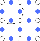
(b)

Figure 1: (color online) Sketch of the crystal structures discussed in this work: (a) 1D chain, and (b) 2D plane, consisting of light atoms (filled circles) intercalated between heavy atoms (empty circles). In the absence of carriers, the ionic potential of a light atom is a simple harmonic well. In the presence of a carrier, the ionic potential of the light atom hosting it remains an even function of its longitudinal displacement, so the linear e-ph coupling vanishes. In suitable conditions the effective ionic potential becomes a double well (see text for more details).

The crystal structures of interest are illustrated in Fig. 1(a) for 1D, and Fig. 1(b) for 2D cases. The 3D crystal would have a perovskite structure but we do not discuss it explicitly because, as we show below, dimensionality plays no role in determining the polaron properties.

The undoped compound is an insulator made of light atoms, shown as filled circles, intercalated between heavy ones, shown as empty circles. To zeroth order, the vibrations of the heavy atoms can be ignored while those of the light atoms are described by independent harmonic oscillators $\mathcal{H}_{\text{ph}}=\Omega\sum_{i}b_{i}^{\dagger}b_{i}^{\phantom{\dagger}}$, where $b_{i}$ annihilates a phonon at the $i^{th}$ light atom. (We set the mass of the light ions $M=1$, and also $\hbar=1$). In reality there is weak coupling between these oscillators giving rise to a dispersive optical phonon branch. However, the dispersion can be ignored if its bandwidth is small compared to all other energy scales. We do so in the following.

Consider now the addition of a carrier. If it occupies orbitals centered on the heavy atoms, its coupling to the oscillations of the light atoms is described by breathing-mode coupling models.bm Here we are instead interested in the case where the carrier is located on the light atoms. Such is the situation for a CuO₂ plane as shown in Fig. 1(b), since the parent compound is a charge-transfer insulatorZSA so that upon doping, the holes reside on the light O sites (of course, there are additional complications due to the magnetic order of the Cu spins; we ignore these degrees of freedom in the following). The carrier moves through nearest-neighbor hopping between light atoms: $\hat{T}=-t\sum_{\langle i,j\rangle}\left(c_{i}^{\dagger}c_{j}^{\phantom{\dagger}}+h.c.\right)$, where $c_{i}$ is the carrier annihilation operator at light atom $i$.

Given the symmetric equilibrium location of the light ion hosting the carrier between two heavy ions, it is clear that the e-ph coupling cannot be linear in the displacement $\delta x_{i}$ of that light ion: the sign of the displacement cannot matter. Thus, e-ph coupling in such a material is not described by a Holstein model. This assertion is supported by detailed modelling. For simplicity, we assume that the interactions with the neighboring heavy atoms are dominant (longer-range interactions can be easily included but lead to no qualitative changes). There are, then, two distinct contributions to the e-ph coupling:

Electrostatic coupling:

The carrier changes the total charge of the light ion it resides on. If the distance between adjacent light and heavy ions is $d$, and if $U(x)$ is their additional Coulomb interaction due to the carrier, then the potential increases by $U(d+\delta x_{i})+U(d-\delta x_{i})$. This is an even function and thus has no linear (or any odd) terms in $\delta x_{i}$. The coefficient of the quadratic term $(\delta x_{i})^{2}$ can be either positive or negative, depending on the charge of the carrier (electron or hole).

Hybridization:

Even though charge transport is assumed to take place in a light atom band, there is always some hybridization $t_{lh}$ allowing the carrier to hop onto an adjacent heavy ion. If $\Delta$ is the corresponding energy increase, assumed to be large, then the carrier can lower its on-site energy by $-t_{lh}^{2}/\Delta$ through virtual hopping to a nearby heavy ion and back. The hopping $t_{lh}$ depends on the distance between ions; for small displacements $t_{lh}(\delta x)\approx t_{lh}(1+\alpha\delta x)$ where $\alpha$ is some material-specific constant. Because the light ion is centered between two heavy ions, such contributions add to $\frac{-t_{lh}^{2}}{\Delta}\left[(1+\alpha\delta x)^{2}+(1-\alpha\delta x)^{2}\right]=\frac{-2t_{lh}^{2}}{\Delta}\left[1+\alpha^{2}(\delta x)^{2}\right].$ The potential is again even in $\delta x$. In this case, the coefficient of the quadratic term is always negative.

Given that $\delta x_{i}\sim b_{i}+b_{i}^{\dagger}$, it follows that the largest (quadratic) contribution to the e-ph coupling for such a crystal has the general form:

$$\mathcal{H}^{(2)}_{\text{e-ph}}=g_{2}\sum_{i}c_{i}^{\dagger}c_{i}\left(b_{i}+b_{i}^{\dagger}\right)^{2}$$

where all prefactors have been absorbed into the energy scale $g_{2}$, and the sum is over all light ions. From the analysis above we know that $g_{2}$ may have either sign.

Physically, $\mathcal{H}^{(2)}_{\text{e-ph}}$ shows that the presence of a carrier modifies the curvature of its ion’s lattice potential, and thus changes the phonon frequency at that site from $\Omega$ to $\Omega_{\text{at}}=\sqrt{\Omega^{2}+4\Omega g_{2}}$. If $g_{2}>0$ then $\Omega_{\text{at}}>\Omega$, making phonon creation more costly. As we show in Appendix C, this leads to a rather uninteresting large polaron with very weakly renormalized properties. This is why in the following we focus on the case with $g_{2}<0$.

For sufficiently negative $g_{2}$, $\Omega_{\text{at}}$ vanishes or becomes imaginary, i.e. the lattice is unstable. This is unphysical; in reality the bare ionic potential contains higher order terms that stabilize the lattice. This means that for $g_{2}<0$ we must include anharmonic (quartic) terms in the phonon Hamiltonian and, for consistency, also in the e-ph coupling, so that

$$\mathcal{H}_{\text{ph}} =\Omega\sum_{i}b_{i}^{\dagger}b_{i}^{\phantom{\dagger}}+\Theta\sum_{i}(b_{i}^{\dagger}+b_{i}^{\phantom{\dagger}})^{4}$$

$$\mathcal{H}^{(4)}_{\text{el-ph}} =\sum_{n\in\{2,4\}}g_{n}\sum_{i}c_{i}^{\dagger}c_{i}^{\phantom{\dagger}}(b_{i}^{\dagger}+b_{i}^{\phantom{\dagger}})^{n},$$

where $\Theta$ is the scale of the anharmonic corrections. In physical situations $\Theta\ll\Omega$ and $0<g_{4}\ll|g_{2}|$, or the Taylor expansions would not be sensible starting points.

The anharmonic terms in $\mathcal{H}_{\text{ph}}$ make the total Hamiltonian unwieldy, because the phonon vacuum $|0\rangle$ is no longer the undoped ground-state, and the new undoped ground state $\ket{\tilde{0}}$ has no simple analytical expression. In order to be able to proceed with an analytical approximation, we argue that these terms can be absorbed into the e-ph coupling; this is a key approximation of the model. The reasoning is as follows: At those lattice sites that do not have a carrier, the quartic terms have little effect if $\theta\ll\Omega$. This statement is verified by exact diagonalization of $\mathcal{H}_{\text{ph}}$. Results are shown in Fig. 2 where we plot the overlap $O=|\langle 0|{\tilde{0}}\rangle|^{2}$ (per site) between the undoped ground-states with and without anharmonic corrections, as well as the average number of phonons at a site of the undoped lattice. Even for unphysically large values $\Theta/\Omega\sim 1$, the overlap $O$ remains close to 1 while $N_{\text{ph}}\ll 1$, showing that the undoped ground-state has not changed significantly in the presence of anharmonic corrections. From now we ignore these corrections at sites without an additional carrier.

Figure 2: (a) Overlap between the undoped ground-states with and without anharmonic corrections, and (b) the average number of phonons per site in the undoped system, due to anharmonic corrections, as a function of $\theta/\Omega$.

However, for sites that have a carrier present, we cannot ignore the anharmonic term: As discussed, it is crucial for stabilizing the lattice. Since this term is similar to the quartic term in the e-ph coupling, they can both be grouped together, resulting in the approximate Hamiltonian for our crystal:

$$\mathcal{H}=\hat{T}+\Omega\sum_{i}b_{i}^{\dagger}b_{i}^{\phantom{\dagger}}+g_{2}\sum_{i}c_{i}^{\dagger}c_{i}^{\phantom{\dagger}}\left(b_{i}^{\dagger}+b_{i}^{\phantom{\dagger}}\right)^{2}\\ +(g_{4}+\Theta)\sum_{i}c_{i}^{\dagger}c_{i}^{\phantom{\dagger}}\left(b_{i}^{\dagger}+b_{i}^{\phantom{\dagger}}\right)^{4}$$ (1)

with an effective quartic e-ph coupling term $g_{4}+\Theta$, which from now on we will simply call $g_{4}$. This is the Hamiltonian that we investigate in this work.

Before proceeding, let us review what we are neglecting when we discard the anharmonic corrections at the unoccupied sites. Besides ignoring the change in the undoped ground state from $|0\rangle$ to $|{\tilde{0}}\rangle$ (which is a reasonable approximation if $\theta/\Omega\ll 1$, as discussed), we also assume that only the e-ph coupling can change the number of phonons in the system, whereas in the full model the phonon number is also changed by anharmonic corrections. This latter approximation is valid if the timescale for anharmonic phonon processes $\tau_{4}\sim 1/\Theta$ is much longer than the characteristic polaron timescale $\tau_{p}\sim tm/m^{*}$, where $m^{*}$ is the effective polaron mass.

Let us briefly summarize the basic properties of the lattice potential, which equals $V_{e}(\delta x)=\Omega^{2}(\delta x)^{2}/2$ for sites without an extra carrier, and $V_{c}(\delta x)=\Omega_{\text{at}}^{2}(\delta x)^{2}/2+4\Omega^{2}g_{4}(\delta x)^{4}$ for sites with one carrier. If $g_{2}>-\Omega/4$, the first term describes a harmonic well with frequency $\Omega_{\text{at}}$ and $V_{c}(\delta x)$ describes a single well centered at $\delta x=0$. If $g_{2}<-\Omega/4$, however, $\Omega_{\text{at}}$ becomes purely imaginary. In this case, $V_{c}(\delta x)$ becomes a double-well potential with a local maximum at $\delta x=0$. The two wells are centered at $\pm x_{\text{eq}}=\pm\sqrt{\frac{-\Omega-4g_{2}}{16\Omega g_{4}}}.$ For $\delta x\approx\pm x_{\text{eq}}$ we obtain $V_{c}(\delta x)\approx V(x_{\text{eq}})-\Omega_{\text{at}}^{2}(\delta x\mp x_{\text{eq}})^{2}$, which locally describes a harmonic well of frequency $\Omega_{\text{eff}}^{2}=-2\Omega_{\text{at}}^{2}$. Interestingly, this is independent of $g_{4}$, whose only role is to control the location and depth of the two wells (they are further apart and deeper for smaller $g_{4}$).

III Formalism

We want to find the single particle Green’s function $G(k,\omega)=\braket{0}{c_{k}^{\phantom{\dagger}}\hat{G}(\omega)c_{k}^{\dagger}}{0}$, where $\hat{G}(\omega)=[\omega-\mathcal{H}+i\eta]^{-1}$ is the resolvent of Hamiltonian (1). From this, we can obtain all the polaron’s ground state properties as well as its dispersion.(Goodvin et al., 2006)

Grouping terms in the Hamiltonian according to how they affect the phonon number, we rewrite $\mathcal{H}=\mathcal{H}_{0}+\mathcal{H}_{p}+\mathcal{H}_{2}+\mathcal{H}_{4}$ with $\mathcal{H}_{0}=\hat{T}+\Omega\sum_{i}b_{i}^{\dagger}b_{i}+g_{2}+3g_{4}$ and $\mathcal{H}_{p}=\sum_{i}n_{i}b_{i}^{\dagger}b_{i}(2g_{2}+6g_{4}+6g_{4}b_{i}^{\dagger}b_{i})$ do not change the number of phonons, while $\mathcal{H}_{2}=\sum_{i}n_{i}\left[(g_{2}+6g_{4})(b_{i}^{\dagger,2}\!+b_{i}^{2})+4g_{4}(b_{i}^{\dagger,3}b_{i}+b_{i}^{\dagger}b_{i}^{3})\right]$ and $\mathcal{H}_{4}=g_{4}\sum_{i}n_{i}\left(b_{i}^{\dagger,4}+b_{i}^{4}\right)$ change it by $\pm 2$ and $\pm 4$, respectively. The constant $g_{2}+3g_{4}$ in $\mathcal{H}_{0}$ is absorbed into $\omega$ in the following derivations, but plots of the spectral weight will show actual energies.

One important property of this Hamiltonian is that it preserves the phonon number parity on each site: because its terms only change the number of phonons by multiples of two, any eigenstate is a sum of basis states having only even (or only odd) number of phonons. The Hilbert space can thus be divided into an even and an odd (phonon number) sector, which can be diagonalized separately. We emphasize that this symmetry is different from the parity symmetry under a global lattice inversion $\vec{r}\rightarrow-\vec{r}$. The latter has been studied extensively for the linear Holstein model,linear_symmetry where it was shown that polaron states with total momentum $K=0,\pi$ have well defined (spatial) parity. The phonon number parity, on the other hand, corresponds to a unitary transformation $b_{i}^{\dagger}\rightarrow-b_{i}^{\dagger}$, i.e., a local inversion of the phonon coordinates. The number parity symmetry also correlates with the local spatial parity of the ions, since the spatial parity operator for site $i$ can be written as $\hat{P}_{i}=\exp(i\pi b_{i}^{\dagger}b_{i})$.

III.1 The even sector

We compute the Green’s function via the same continued matrix fractions methodMöller et al. (2012) previously used by us to compute the Green’s function of a generalized Holstein model with linear and higher-order termsAdolphs and Berciu (2013) within the framework of the momentum average (MA) approximation. This approximation was shown to be highly accurate for models with Holstein coupling.Berciu (2006); Goodvin et al. (2006) The reasons for this (such as obeying exact sum rules) can be verified to hold for this model, too. To be specific, here we implement the MA⁽²⁾ flavor which allows us to also locate the continuum lying above the polaron band.Berciu and Goodvin (2007)

We begin our derivation by dividing the Hamiltonian into $\mathcal{H}=\mathcal{H}_{0}+\mathcal{H}_{1}$ with $\mathcal{H}_{1}=\mathcal{H}_{p}+\mathcal{H}_{2}+\mathcal{H}_{4}$. Using Dyson’s identity $\hat{G}(\omega)=\hat{G}_{0}(\omega)+\hat{G}(\omega)\mathcal{H}_{1}\hat{G}_{0}(\omega)$, where $\hat{G}_{0}(\omega)=[\omega-\mathcal{H}_{0}+i\eta]^{-1}$, we obtain

$$G(k,\omega)=G_{0}(k,\omega)\Big{[}1+\\ \sum_{i}\frac{e^{ikR_{i}}}{\sqrt{N}}(g_{2}+6g_{4})F_{1}(k,\omega;i,i)+g_{4}F_{2}(k,\omega;i,i)\Big{]}$$ (2)

with $F_{n}(k,\omega;i,j)=\braket{0}{c_{k}\hat{G}(\omega)c_{i}(b_{i}^{\dagger})^{2n-2}(b_{j}^{\dagger})^{2}}{0}$ being the generalized propagator for a system with $2n$ phonons in total, $2n-2$ of them on site $i$ with the other two on site $j$. The difference between MA⁽²⁾ and the original MA, which we also call MA⁽⁰⁾, is that for $F_{1}$ we also use its exact equation of motion (EOM),

$$F_{1}(k,\omega;i,j)=G(k,\omega;j)G_{0}(j-i,\omega-2\Omega)(2g_{2}+12g_{4})+F_{1}(k,\omega;j,j)G_{0}(j-i,\omega-2\Omega)(4g_{2}+36g_{4})\\ +8g_{4}F_{2}(k,\omega;j,j)G_{0}(j-i,\omega-2\Omega)+\sum_{l}G_{0}(l-i,\omega-2\Omega)\left[F_{2}(k,\omega;l,j)(g_{2}+6g_{4})+F_{3}(k,\omega;l,j)g_{4}\right].$$ (3)

which is obtained by applying Dyson’s identity again, and introducing $G(k,\omega;j)=\braket{0}{c_{k}^{\phantom{\dagger}}\hat{G}(\omega)c_{j}^{\dagger}}{0}$ and $G_{0}(j-i,\omega)=\braket{0}{c_{j}^{\phantom{\dagger}}\hat{G}_{0}(\omega)c_{i}^{\dagger}}{0}$. The equations of motion for the $F_{n}$ propagators with $n\geq 2$ are approximated by replacing the free propagator $G_{0}(j-i,\omega-2n\Omega)\rightarrow\delta_{i,j}\bar{g}_{0}(\omega-2n\Omega)$, where $\bar{g}_{0}(\omega)={1\over N}\sum_{k}G_{0}(k,\omega)$ is the momentum averaged free propagator. At low energies this is a good approximation because $G_{0}(j-i,\omega-2n\Omega)$ decays exponentially with the distance $|j-i|$ if $\omega-2n\Omega<-2dt$ in $d$ dimensions. This is also justified by the variational meaning of the MA approximations, discussed at length elsewhere.bar ; Berciu and Goodvin (2007) (Basically, MA⁽²⁾ assumes that all phonons in the cloud are at the same site but also allows for a pair of phonons to be created at a site away from the cloud).

The resulting EOMs are different depending on whether $i=j$ or $i\not=j$. If we define $F_{n}^{=}(k,\omega;i)=F_{n}(k,\omega;i,i)$ and $F_{n}^{\neq}(k,\omega;i,j)=F_{n}(k,\omega;i,j)$ for $i\neq j$, we obtain

$$F_{n}^{=}(k,\omega;i)=\bar{g}_{0}(\omega-2n\Omega)\Big{[}F_{n-2}^{=}(2n)^{\bar{4}}g_{4}+F_{n-1}^{=}\left((g_{2}+6g_{4})(2n)^{\bar{2}}+4g_{4}(2n)^{\bar{3}}\right)+\\ (4ng_{2}+12ng_{4}+24n^{2}g_{4})F_{n}^{=}+(g_{2}+6g_{4}+8ng_{4})F_{n+1}^{=}+g_{4}F_{n+2}^{=}\Big{]}.$$ (4)

$$F_{n}^{\neq}(k,\omega;i,j)=\bar{g}_{0}(\omega-2n\Omega)\Big{[}g_{4}(2n-2)^{\bar{4}}F_{n-2}^{\neq}+\left((g_{2}+6g_{4})(2n-2)^{\bar{2}}+(2n-2)^{\bar{3}}\cdot 4g_{4}\right)F_{n-1}^{\neq}+\\ \left[2(2n-2)g_{2}+12(n-1)g_{4}+6(2n-2)^{2}g_{4}\right]F_{n}^{\neq}+\left[g_{2}+6g_{4}+4(2n-2)g_{4}\right]F_{n+1}^{\neq}+g_{4}F_{n+2}^{\neq}\Big{]}$$ (5)

where we use the notation $x^{\bar{n}}=x!/(x-n)!$. We also omitted the arguments from the $F_{n}$ appearing on the right hand sides, as they remain unchanged.

These EOMs connect generalized Green’s functions $F_{n}$ with $F_{n\pm 1}$ and $F_{n\pm 2}$. We reduce this to a first order recurrence relationAdolphs and Berciu (2013) by introducing vectors $W_{n}^{=}=(F_{2n}^{=},F_{2n+1}^{=})$ and analogously for $W_{n}^{\neq}$. Below, we write $W_{n}$ without the index $=$ or $\neq$ for results that apply to both $W_{n}^{=}$ and $W_{n}^{\neq}$. By inserting the EOMs into the definition of $W_{n}$, we obtain a matrix EOM for the $W_{n}$,

$$\gamma_{n}W_{n}=\alpha_{n}W_{n-1}+\beta_{n}W_{n+1}.$$ (6)

The coefficients of these matrices are read off from the EOM for the $F_{n}$. They are listed in appendix A.1.

Using the fact that $\lim_{n\rightarrow\infty}A_{n}=0$ we can showAdolphs and Berciu (2013) that $W_{n}=A_{n}W_{n-1}$ with $A_{n}=\left[\gamma_{n}-\beta_{n}A_{n+1}\right]^{-1}\alpha_{n}$. By introducing a suitably large cut-off $N$ where we set $A_{N+1}=0$, we can compute all $A_{n}$ with $n\leq N$ as continued matrix fractions. Knowledge of $A_{1}$ allows us to express $F_{2}$ and $F_{3}$ in terms of $F_{1}$ and $F_{0}=G$. Following a series of steps presented in appendix A.2, we obtain a closed equation for $F_{1}$ in terms of $G$, which we then finally use to compute $G$. The end result of these manipulations is the self energy

$$\Sigma(\omega)=\frac{(g_{2}+6g_{4}+A_{1}^{=}|_{12}g_{4})\tilde{g}_{0}(\omega)a_{0}^{=}}{1-\tilde{g}_{0}(\omega)(a_{1}^{=}-a^{\neq})}+g_{4}A_{1}^{=}|_{11}.$$

with $\tilde{g}_{0}(\omega)=\bar{g}_{0}(\omega-2\Omega-a^{\neq}$) and the other coefficients defined in appendix A.2. The independence of the self-energy on momentum is the consequence of the local form of the coupling and of the non-dispersive phonons, similar to the MA results for the Holstein model.Berciu and Goodvin (2007) Momentum-dependence would be acquired in a higher flavor of MA, but is likely to be weak. Finally, the Green’s function is:

$$G(k,\omega)=\frac{1}{\omega-\epsilon_{k}-\Sigma(\omega)+i\eta}.$$ (7)

One can now use the matrices $A_{n}$ to generate the generalized propagators $F_{n}$, which allow one to reconstruct the entire polaron wavefunction (within this variational space).Can For the quantities of interest here, however, the single-particle Green’s function suffices.

III.2 The odd sector

Here we calculate the Green’s function for a state that already has a phonon in the system. Since the phonon number can only change by $2$ or $4$, this single phonon can never be moved to another site, so it is natural to compute the Green’s function in real space. The most general such real space Green’s function is:

$$G_{ijl}(\omega)=\braket{0}{b_{l}^{\phantom{\dagger}}c_{j}^{\phantom{\dagger}}\hat{G}(\omega)c_{i}^{\dagger}b_{l}^{\dagger}}{0}.$$

Applying the Dyson identity leads to the EOM

$$G_{ijl}(\omega)=G_{0}(j-i,\omega-\Omega)\\ +\sum_{i^{\prime}}G_{0}(i^{\prime}-i,\omega-\Omega)\braket{0}{b_{l}^{\phantom{\dagger}}c_{j}^{\phantom{\dagger}}\hat{G}(\omega)\mathcal{H}_{1}c_{i^{\prime}}^{\dagger}b_{l}^{\dagger}}{0}.$$

We then split the sum over all lattice sites into a term $i^{\prime}=l$ where the electron is on the same site as the extra phonon, and a sum over all the other sites. The subsequent steps are very similar to those for the even-sector Green’s function. We summarize them in Appendix B, where we also discuss how various propagators that enforce translational symmetry – i.e. propagators defined in momentum space – can be obtained from these real-space Green’s functions.

The end result for the real-space Green’s functions is $G_{ijl}(\omega)=G_{0}(j-i,\tilde{\omega})+G_{0}(l-i,\tilde{\omega})G_{0}(j-l,\tilde{\omega})(a^{=}_{\text{o}}-a^{\neq}_{\text{o}})[1-\bar{g}_{0}(\tilde{\omega})(a^{=}_{\text{o}}-a^{\neq}_{\text{o}})]^{-1}$ where $\tilde{\omega}=\omega-a^{\neq}_{\text{o}}-\Omega$. The coefficients $a^{=}_{o}$ and $a^{\neq}_{o}$ are listed in appendix B.

IV Results

IV.1 Atomic limit: $t=0$

We begin our analysis with the atomic limit since it is a good starting point for understanding the properties of the small polaron, which is the more interesting regime. However, we note an important distinction between the Holstein model and our double-well model. In the former, the atomic limit is the infinite-coupling limit. In the latter, $g_{4}$ sets an additional energy scale. Thus, the atomic limit is not the same as the strong coupling limit; the latter also requires that $g_{4}/|g_{2}|$ be small.

Before doing any computations, we can describe some general features of the spectrum. As already discussed, the phonon component of the wavefunctions has either even or odd phonon number parity. Since this is due to the spatial symmetry in the local ionic displacement, in any eigenstate the ion is equally likely to be found in either well. As usual, the ground state has even symmetry since it has no nodes in its wavefunction. Subsequent eigenstates always have one more node than the preceding eigenstate, so states with even and odd parity alternate. The exception is the limit of infinite well separation, $g_{4}/|g_{2}|\rightarrow 0^{+}$, where the $2n^{th}$ and $2n+1^{st}$ eigenstates become degenerate. The system can then spontaneously break parity to have the ion definitely located in the left or in the right well, like in a ferroelectric. For a finite $g_{4}$ this is not possible in the single carrier limit, but it can be achieved at finite carrier concentration through spontaneous symmetry breaking.

As discussed, our results are obtained with MA. In the atomic limit MA is exactBerciu (2006) because for $t=0$ the free propagator is diagonal in real-space so the terms ignored by MA vanish. Thus, MA results must be identical here to those obtained by other exact means. To check our implementation of MA, we used exact diagonalization (ED) with up to a few thousand phonons; this suffices for an accurate computation of the first few eigenstates. ED and MA results agree, as required.

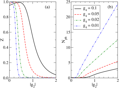
Figure 3: (color online) Polaron ground-state properties in the atomic limit, for several values of the $g_{4}$: a) quasiparticle weight, and b) average number of phonons in the phonon cloud. Other parameters are $\Omega=0.5,t=0$.

Figure 3 shows the ground-state quasiparticle weight $Z$ (the overlap between the polaron ground-state and the non-interacting carrier ground-state), and the ground-state average number of phonons in the cloud, $N_{\text{ph}}$, as a function of $g_{2}<0$, for various values of $g_{4}$. $Z$ has an interesting behavior. At $g_{2}=0$ it is slightly below $1$ because of the quartic terms. As $|g_{2}|$ is increased, $Z$ first rises towards a value close to $1$ and then sharply drops. This turnaround is caused by the terms that involve both $g_{2}$ and $g_{4}$, i.e. $(2g_{2}+6g_{4})\sum_{i}n_{i}b_{i}^{\dagger}b_{i}$ from $\mathcal{H}_{p}$ and $(g_{2}+6g_{4})\sum_{i}n_{i}(b_{i}^{\dagger,2}+b_{i}^{2})$ from $\mathcal{H}_{2}$. Starting from $g_{2}=0$ and making it increasingly more negative will at first decrease these coefficients, thereby renormalizing the ground state less. For even more negative $g_{2}$, however, $Z$ decreases sharply as the absolute value of these coefficients increases; this is paralleled by a strong increase in $N_{\text{ph}}$. Based on this argument, the peak in $Z$ should occur for $-6g_{4}<g_{2}<-3g_{4}$, which is indeed the case. The strong-coupling limit of a small polaron (corresponding to small $Z$, large $N_{\text{ph}}$ values) is therefore reached either by increasing $|g_{2}|$ or by lowering $g_{4}$.

While this allows us to conclude that in the atomic limit the crossover into the small polaron regime occurs at $\frac{g_{2}}{3g_{4}}\approx-1.5$, it also illustrates the difficulty in defining an effective coupling for this model. For the Holstein model, the dimensionless effective coupling $\lambda$ is the ratio between the ground-state energies in the atomic limit and in the free electron limit; the crossover to the small polaron regime occurs at $\lambda\sim 1$. For the double-well model the introduction of an effective coupling is not as straightforward, because the atomic limit has vastly different properties depending on the ratio $g_{2}/g_{4}$, so comparing the energy in this limit to that of a free electron is not sufficient. (Moreover, there is no analytic expression for the ground state energy of the double well potential). For these reasons, we continue to use the bare coupling parameters $g_{2}$ and $g_{4}$ to characterize our model.

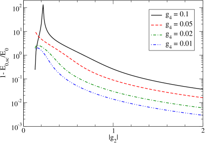
Figure 4: (color online) Relative error in the ground state energy when computed in the semiclassical approximation (see text for details). The coupling $g_{2}<-\Omega/4$ is restricted to values for which there is a double-well potential. Other parameters are like in Fig. 3.

For strong coupling, we can accurately estimate the ground state energy by using the barrier depth and effective harmonic frequency of the double-well potential, $E_{0,\text{sc}}=V_{c}(x_{\text{eq}})+\Omega_{\text{eff}}/2$. Fig. 4 shows the relative error of this estimate, which indeed decreases as parameters move deeper into the small polaron regime. Since here the tunnelling between the two wells also becomes increasingly smaller, one may think that we can describe this regime accurately by assuming that the carrier becomes localized in one of the wells (thus breaking parity), i.e. that we can approximate the full lattice potential as being a single harmonic well centered at either $x_{\text{eq}}$ or $-x_{\text{eq}}$. Of course, the latter situation can be modelled with a linear Holstein model.

It turns out that this is not the case. In the standard Holstein model, the charge carrier cannot change the curvature of the lattice potential and thus cannot account for the difference between $\Omega$ and $\Omega_{\text{eff}}$. To account for the change in the curvature of the well, one would have to consider at least a Holstein model with both linear and quadratic e-ph coupling terms. Although it is possible to find effective parameters $g_{1,\text{eff}}$, $g_{2,\text{eff}}$ and $\Omega_{\text{eff}}$ so that the resulting lattice potential in the presence of the carrier has the same location and curvature as one of the wells of the double-well potential, the corresponding quasi-particle weight $Z_{\text{eff}}$ severely underestimates $Z$. This is because the single well approximation severely overestimates the lattice potential at $x=0$, thereby reducing the overlap between the ground state of the shifted well and that of the original well. We conclude that the double-well coupling cannot be accurately described by a (renormalized) Holstein coupling even in this simplest limit.

IV.2 Finite Hopping

We focus on results from the even sector because it describes states accessible by injecting the carrier in the undoped ground-state. The odd sector is accessed only if the carrier is injected into an excited state with an odd number of phonons present in the undoped system; we briefly discuss this case at the end of the section.

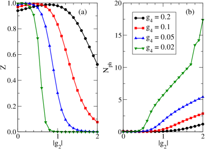
Figure 5: (color online) Polaron ground-state properties in one dimension for various values of the quartic coupling term $g_{4}$ as a function of the quadratic coupling $g_{2}$: a) quasiparticle weight, and b) average number of phonons in the phonon cloud. Other parameters are $t=1$, $\Omega=0.5t$.

We begin by plotting the ground-state values of $Z$ and $N_{\text{ph}}$, for 1D and 2D lattices, in Figs.  5 and 6 respectively. Since the MA self-energy is local, the effective polaron mass $m^{*}=m/Z$, where $m$ is the free carrier mass; we therefore do not plot $m^{*}$ separately. Apart from $t=1$, the parameters are like in Fig. 3. Note that the kinks in the $N_{\text{ph}}$ curves for $g_{4}=0.02$ are not physical; they arise from numerical difficulties in resolving the precise location of the ground state peak when $Z\rightarrow 0$.

Qualitatively, the polaron properties show the same dependence on $g_{2}$ as in the atomic limit, but the shape and location of the turnarounds is slightly modified: As one would expect, the presence of finite hopping counteracts the formation of a robust polaron cloud and increases the quasi-particle weight $Z$ for any given $g_{2}$ and $g_{4}$ when compared to the atomic limit.

The results in one and two dimensions are strikingly similar. The 2D $Z$ is slightly larger than the 1D $Z$, and $N_{\text{ph}}$ in 2D is slightly lower than in 1D. This is expected because in higher dimensions, the polaron formation energy is competing against a larger carrier kinetic energy. These results suggest that dimensionality is not playing a key role for the double-well model, similar to the situation for the Holstein model. This is why we did not consider 3D systems explicitly.

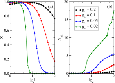
Figure 6: (color online) Polaron ground-state properties in two dimensions for various values of the quartic coupling term $g_{4}$ as a function of the quadratic coupling $g_{2}$: a) quasiparticle weight, and b) average number of phonons in the phonon cloud. Other parameters are $t=1$, $\Omega=0.5t$.

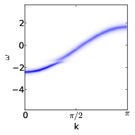
(a) $g_{2}=-0.5$

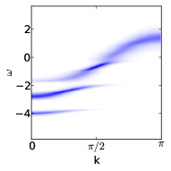
(b) $g_{2}=-1$

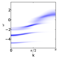
(c) $g_{2}=-1.5$

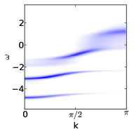
(d) $g_{2}=-2$

Figure 7: $A(k,\omega)$ in 1D, for $g_{4}=0.05$, $\Omega=0.5$ and $t=1$, for various values of $g_{2}$.

We now move on to discuss the evolution of the spectral weight $A(k,\omega)=-{1\over\pi}\text{Im}G(k,\omega)$ with increasing $|g_{2}|$, at a fixed value of $g_{4}$. This is shown in Fig. 7 for 1D, and in Fig. 8 for 2D. Because the evolution is again qualitatively similar in the two cases, we analyze in more detail the 1D results. Here, at small quadratic coupling $g_{2}=-0.5$, we observe the appearance of a polaron band below a continuum of states. This continuum begins at $E_{0}+2\Omega$, and consists of excited states comprising the polaron plus two phonons far away from it. (In our MA⁽²⁾ approximation, the continuum actually begins at $E_{0}^{\text{MA}^{(0)}}+2\Omega$, not at $E_{0}^{\text{MA}^{(2)}}+2\Omega$, for reasons detailed in Ref. Berciu and Goodvin, 2007).

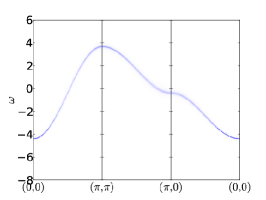
(a) $g_{2}=-0.5$

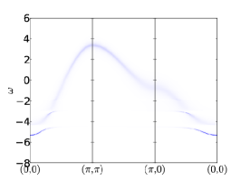
(b) $g_{2}=-1$

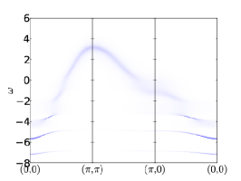
(c) $g_{2}=-1.5$

Figure 8: $A(k,\omega)$ in 2D, for $g_{4}=0.05$, $\Omega=0.5$ and $t=1$, for various values of $g_{2}$.

Note that due to the parity-preserving nature of the Hamiltonian there is no analog of the polaron+one-phonon continuum starting at $E_{0}+\Omega$, which is observed in all linear coupling models. Trying to mimic the results of the double-well coupling with a linear model will, therefore, lead to a wrong assignment for the value of $\Omega$.

At small $|g_{2}|$, the polaron band flattens out just below the polaron+two-phonon continuum. With increasing $|g_{2}|$, its bandwidth decreases as the polaron becomes heavier, and additional bound states appear below the continuum. This is similar to the evolution of the spectrum of a Holstein polaron when moving towards stronger effective coupling.Goodvin et al. (2006) However, as already discussed, this does not mean that the two Hamiltonians can be mapped onto one another.

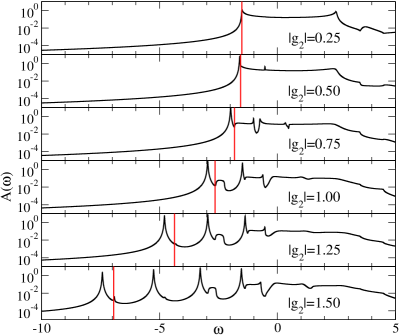
Figure 9: Real-space diagonal spectral function $A_{iii}(\omega)$ at $g_{4}=0.05$ for various values of (negative) $g_{2}$ in one dimension and for $\Omega=0.5$. The $y$-axis has a logarithmic scale. The vertical bars indicate the position of $E_{0}^{\text{even}}+\Omega$.

For completeness, let us also discuss some of the features of the odd sector. In particular, we focus on the local Green’s function $G_{iii}(\omega)$, which can be written as

$$G_{iii}(\omega)=\bar{g}_{0}(\tilde{\omega})+\frac{\bar{g}_{0}(\tilde{\omega})^{2}(a^{=}-a^{\neq})}{1-\bar{g}_{0}(\tilde{\omega})(a^{=}-a^{\neq})}$$

with $\tilde{\omega}=\omega-\Omega-a^{\neq}$. One can verify that $a^{\neq}$ equals the MA⁽⁰⁾ self-energy for the even sector, up to a shift by $\Omega$ of its frequency. The equation for $G_{iii}(\omega)$ then shows that the odd sector spectral function comprises two parts: (i) the first term is just the momentum-averaged spectral function of the even-sector, shifted in energy by $\Omega$ due to the presence of the extra phonon. One can think of these as states where the even-sector polaron does not interact with the extra phonon. This contribution therefore has weight starting from $E_{0}+\Omega$; (ii) the second part describes interactions between the polaron and the extra phonon. An interesting question is whether these can lead to a bound state, i.e. to a new polaron with odd numbers of phonons in its cloud.

This question is answered in Fig. 9 where we plot $A_{iii}(\omega)=-{1\over\pi}\text{Im}G_{iii}(\omega)$ for different values of $|g_{2}|$ and $g_{4}=0.05$, $\Omega=0.5$, $t=1$, in one dimension. The vertical bars indicate the position of $E_{0}+\Omega$, where indeed a continuum begins, as expected from the previous discussion. At sufficiently strong coupling $|g_{2}|$ we find a discrete bound state below that continuum, showing that the polaron can bind the extra phonon. In fact, it is more proper to say that the extra phonon (which is localized somewhere on the lattice) binds the polaron to itself and therefore localizes it. One can think of this as an example of “self-trapping”, except here there is an external trapping agent in the form of the extra phonon.

One might wonder whether this localized bound state in the odd sector could ever be at an energy below the polaron ground-state energy $E_{0}$ of the even sector, i.e. become the true ground-state. This is not the case; as explained above, in the atomic limit the ionic states alternate between even and odd symmetry. Introducing a finite hopping allows the polaron to further lower its energy by delocalizing, but this is only possible in the even sector. Thus, we always expect the even-sector polaron to have an energy below that of this localized state.

As stated before, the two subspaces with even and odd phonon number are never mixed, at least at zero temperature. At finite temperature, the extra charge is inserted not into the phonon vacuum but into a mixed state containing a number of thermally excited phonons. We therefore expect the resulting spectral function to show features of both the even and odd sectors. To be more precise, some spectral weight should be shifted from the even-sector spectral weight to the odd-sector spectral weight as $T$ increases and there is a higher probability to find one or more thermal phonons in the undoped state. We plan to study the temperature depend properties of this double-well coupling elsewhere.

V Summary and Discussions

Here we introduced and motivated a model for purely quadratic e-ph coupling, relevant for certain types of intercalated lattices, wherein the carrier dynamically changes the on-site lattice potential from a single well into a double well potential. All the approximations made in deriving this model were analyzed. In particular, we argued that ignoring the anharmonic lattice terms at the sites not hosting the carrier should be a good approximation. However, a more in-depth numerical analysis might be needed to further validate this assumption.

We used the momentum average approximation to obtain the model’s ground state properties and its spectral function in the single polaron limit, in one and two dimensions. We found that for sufficiently strong quadratic coupling a small polaron forms. Although the polaron behaves somewhat similarly to the polaron of the linear Holstein model, the double-well model cannot be mapped onto an effective linear model: apart from the difference in the location of the continuum in the even sector, the double-well model also has an odd sector that should be visible at finite $T$, and which is entirely absent in the Holstein model. This is due to the double-well potential model’s invariance to local inversions of the ionic coordinate; this symmetry is not found in the Holstein model. The polaron in this odd sector is also qualitatively different from the Holstein polaron, in that it is localized near the additional phonon present in the system when the carrier is injected. Of course, if the assumption of an Einstein mode is relaxed, then the phonon acquires a finite speed and this polaron would become delocalized, as expected for a system invariant to translations. However, this would still be qualitatively different than a regular polaronic solution because this polaron’s dispersion would be primarily controlled by the phonon bandwidth, not the carrier hopping.

Our results suggest that researchers interpreting their measurements from, e.g., angular-resolved photoemission spectroscopy, must carefully consider the nature of their system’s e-ph coupling: if they assume linear coupling where the lattice symmetry calls for a quadratic one, the parameters extracted from fitting to such models will have wrong values.

While we have laid here the basis for a thorough investigation of the properties of the double-well e-ph coupling model, much work remains. We believe that adjusting already existing numerical schemes such as diagrammatic Monte Carlo to this model is straightforward and look forward to a comparison of numerically exact results with our MA results. In addition, there are certain ranges of parameters for which MA is not well-suited, such as the adiabatic limit $\Omega\rightarrow 0$ at weak coupling, or systems with finite carrier densities. We anticipate that these regimes will be explored with a range of numerical and analytical tools, especially the finite carrier regime which should be relevant for modelling ferroelectric materials.

We plan to extend our study of the double-well e-ph coupling beyond the single-polaron limit. We deem especially interesting the parameter range where the lattice potential remains a single well if only one carrier is present, but changes into a double well when a second charge is added. In this case, we anticipate the appearance of a strongly bound bipolaron while the single polarons are relatively light. Such states are not possible in the Holstein model.

Finally, extending our MA treatment to finite temperature should yield interesting insights into the interplay between the two symmetry sectors revealed by the spectral weight.

Appendix A Details for the even-sector

A.1 Coupling matrices

The matrices appearing in Eq. (6) are:

$$\gamma_{n}^{=}|_{11} =1-\bar{g}_{0}(\omega-4n\Omega)(8ng_{2}+24ng_{4}+96n^{2}g_{4})$$

$$\gamma_{n}^{=}|_{12} =-\bar{g}_{0}(\omega-4n\Omega)(g_{2}+6g_{4}+16ng_{4})$$

$$\gamma_{n}^{=}|_{21} =-\bar{g}_{0}(\omega-(4n+2)\Omega)\big{(}(g_{2}+6g_{4})(4n+2)^{\bar{2}}+$$

$$\phantom{=}4g_{4}(4n+2)^{\bar{3}}\big{)}$$

$$\gamma_{n}^{=}|_{22} =1-\bar{g}_{0}(\omega-(4n+2)\Omega)\big{(}(8n+4)g_{2}+$$

$$\phantom{=}(24n+12)g_{4}+24(2n+1)^{2}g_{4}\big{)}$$

$$\alpha_{n}^{=}|_{11} =\bar{g}_{0}(\omega-4n\Omega)(g_{4}(4n)^{\bar{4}})$$

$$\alpha_{n}^{=}|_{12} =\bar{g}_{0}(\omega-4n\Omega)\left((g_{2}+6g_{4})(4n)^{\bar{2}}+4g_{4}(4n)^{\bar{3}}\right)$$

$$\alpha_{n}^{=}|_{21} =0$$

$$\alpha_{n}^{=}|_{22} =\bar{g}_{0}(\omega-(4n+2)\Omega\left(g_{4}(4n+2)^{\bar{4}}\right)$$

$$\beta_{n}^{=}|_{11} =\bar{g}_{0}(\omega-4n\Omega)g_{4}$$

$$\beta_{n}^{=}|_{12} =0$$

$$\beta_{n}^{=}|_{21} =\bar{g}_{0}(\omega-(4n+2)\Omega)(g_{2}+6g_{4}+(16n+8)g_{4})$$

$$\beta_{n}^{=}|_{22} =\bar{g}_{0}(\omega-(4n+2)\Omega)g_{4}$$

The matrices for $\neq$ sector are the same if we substitute $n\rightarrow n-1/2$ everywhere except in the argument of $\bar{g}_{0}(\omega)$.

A.2 Manipulation of the EOMs

We can rewrite the EOM of $F_{1}$ by inserting the matrices $A_{1}^{=}$ and $A_{1}^{\neq}$ and collecting terms. This results in

$$F_{1}(ij)=G_{0}(j-i,\omega-2\Omega)\left[a_{0}^{=}G(j)+a_{1}^{=}F_{1}^{=}(j)\right]\\ +\sum_{l\neq j}G_{0}(l-i,\omega-2\Omega)a^{\neq}F_{1}^{\neq}(lj).$$ (8)

where we omit the arguments $k$ and $\omega$ for shorter notation. We give expressions for the various coefficients below. For now, we rewrite the EOM as

$$F_{1}(ij)=G_{0}(j-i,\omega-2\Omega)\\ \times\left[a_{0}^{=}G(j)+(a_{1}^{=}-a_{1}^{\neq})F_{1}^{=}(j)\right]\\ +\sum_{l}G_{0}(l-i,\omega-2\Omega)a^{\neq}F_{1}(lj).$$ (9)

Defining $G_{0}(\omega)_{ij}:=G_{0}(j-i,\omega)$, we can write this as a matrix product:

$$\sum_{l}\left[\delta_{il}-a^{\neq}G_{0}(\omega-2\Omega)_{il}\right]F_{1}(lj)=\\ G_{0}(\omega-2\Omega)_{ij}\left[a_{0}^{=}G(j)+(a_{1}^{=}-a_{1}^{\neq})F_{1}(jj)\right].$$

We multiply this from the left with $G_{0}^{-1}(\omega-2\Omega)$ and obtain

$$\sum_{l}\left[G_{0}^{-1}(\omega-2\Omega)_{rl}-a^{\neq}\delta_{rl}\right]F_{1}(lj)=\\ \delta_{rj}\left[a_{0}^{\neq}G(j)+(a_{1}^{=}-a^{\neq})F_{1}(jj)\right].$$

Next, we use the fact that $G_{0}^{-1}(\omega-2\Omega)_{rl}=\delta_{rl}(\omega-2\Omega)-\hat{H}_{rl}$, so subtracting $a^{\neq}\delta_{rl}$ from this just shifts its frequency to obtain $G_{0}^{-1}(\omega-2\Omega-a^{\neq})_{rl}$. As a result:

$$F_{1}(ij)=G_{0}(\omega-2\Omega-a^{\neq})_{ij}\\ \times\left[a_{0}^{=}G(j)+(a_{1}^{=}-a_{1}^{\neq})F_{1}(jj)\right].$$

Since in the EOM for $G$ we only require $F_{1}(jj)$, we solve for that diagonal element and obtain

$$F_{1}(jj)=\frac{\bar{g}_{0}(\omega-2\Omega-a^{\neq})a_{0}^{=}G(j)}{1-\bar{g}_{0}(\omega-2\Omega-a^{\neq})(a_{1}^{=}-a_{1}^{\neq})}.$$

The coefficients are obtained by just inserting the appropriate matrices $A_{n}$ into the EOM and collecting terms:

$$a_{0}^{=} =2g_{2}+12g_{4}+(g_{2}+14g_{4})A_{1}^{=}|_{11}+g_{4}A_{1}^{=}|_{21}$$

$$a_{1}^{=} =4g_{2}+36g_{4}+(g_{2}+14g_{4})A_{2}^{=}|_{12}+g_{4}A_{2}^{=}|_{22}$$

$$a^{\neq} =(g_{2}+6g_{4})A_{1}^{\neq}|_{12}+g_{4}A_{1}^{\neq}|_{22}$$

Finally, $F_{1}(jj)$ are used in Eq. (2) to obtain $G(k,\omega)$.

Appendix B Details for the odd-sector

B.1 Equations of Motion

Starting from the EOM for $G_{ijl}(\omega)$, we let $\mathcal{H}_{1}$ act on the states in those sums, to find for the diagonal state:

$$\mathcal{H}_{1}c_{l}^{\dagger}b_{l}^{\dagger}\ket{0}=(2g_{2}+12g_{4})c_{l}^{\dagger}b_{l}^{\dagger}\ket{0}\\ +(g_{2}+10g_{4})c_{l}^{\dagger}b_{l}^{\dagger,3}\ket{0}+g_{4}c_{l}^{\dagger}b_{l}^{\dagger,5}\ket{0}$$

while for the off-diagonal ones:

$$\mathcal{H}_{1}c_{i^{\prime}}^{\dagger}b_{l}^{\dagger}\ket{0}=(2g_{2}+6g_{4})c_{i^{\prime}}^{\dagger}b_{l}^{\dagger}\ket{0}\\ +(g_{2}+6g_{4})c_{i^{\prime}}^{\dagger}b_{l}^{\dagger,2}b_{l}^{\dagger}\ket{0}+g_{4}c_{i^{\prime}}^{\dagger}b_{l}^{\dagger,4}b_{l}^{\dagger}\ket{0}.$$

We now define the generalized Green functions as:

$$F_{n}(k,i,j,\omega)=\braket{k}{\hat{G}(\omega)c_{i}b_{i}^{\dagger,2n}b_{j}}{0}$$

so we always have the extra phonon at site $j$. The equation of motion for $G$ then becomes: $G_{ijl}(\omega)=G_{0}(j-i,\omega-\Omega)+\big{[}(2g_{2}+12g_{4})F_{0}^{=}(l)+(g_{2}+10g_{4})F_{1}^{=}(l)+g_{4}F_{2}^{=}(l)\big{]}G_{ill}+\sum_{i^{\prime}\not=l}\Big{[}(2g_{2}+6g_{4})F_{0}^{\neq}(i^{\prime},l)+(g_{2}+6g_{4})F_{1}^{\neq}(i^{\prime},l)+g_{4}F_{2}^{\neq}(i^{\prime},l)\Big{]}G_{0}(i^{\prime}-i,\omega-\Omega).$ Again, we start by separating the cases $F_{n}^{=}$ and $F_{n}^{\neq}$. The resulting equations of motion for $F_{n}^{=}$ are like those of the even-sector $F_{n}^{=}$ with $n\rightarrow n+1/2$, while those for $F_{n}^{\neq}$ are like those of the even-sector $F_{n}^{\neq}$ with $n\rightarrow n+1$.

In the spirit of MA⁽²⁾, only the EOM for $G$, which already has one phonon present, is kept exact, while in the EOMs for all the $F_{n}$ with $n\geq 1$ we approximate $G_{0}(i-j,\omega)\rightarrow\delta_{ij}\bar{g}_{0}(\omega)$. We introduce matrices $W_{n}=(F_{2n-1},F_{2n})$. Again we obtain an equation like Eq. (6), where now:

$$\gamma^{=}_{11} =1-\bar{g}_{0}(\omega-(4n-1)\Omega)((4n-1)(2g_{2}+6g_{4}$$

$$\phantom{=}+6g_{4}(4n-1))$$

$$\gamma^{=}_{12} =-\bar{g}_{0}(\omega-(4n-1)\Omega)\left(g_{2}+6g_{4}+4g_{4}(4n-1)\right)$$

$$\gamma^{=}_{21} =-\bar{g}_{0}(\omega-(4n+1)\Omega)\Big{(}(4n+1)^{\bar{2}}(g_{2}+6g_{4})$$

$$\phantom{=}+(4n+1)^{\bar{3}}\cdot 4g_{4}\Big{)}$$

$$\gamma^{=}_{22} =1-\bar{g}_{0}(\omega-(4n+1)\Omega)(4n+1)$$

$$\phantom{=}\times\left(2g_{2}+6g_{4}+6g_{4}(4n+1)\right)$$

$$\alpha^{=}_{11} =\bar{g}_{0}(\omega-(4n-1)\Omega)(4n-1)^{\bar{4}}g_{4}$$

$$\alpha^{=}_{12} =\bar{g}_{0}(\omega-(4n-1)\Omega)$$

$$\phantom{=}\times\left((4n-1)^{\bar{2}}(g_{2}+6g_{4})+(4n-1)^{\bar{3}}\cdot 4g_{4}\right)$$

$$\alpha^{=}_{21} =0$$

$$\alpha^{=}_{22} =\bar{g}_{0}(\omega-(4n+1)\Omega)(4n+1)^{\bar{4}}g_{4}$$

$$\beta^{=}_{11} =\bar{g}_{0}(\omega-(4n-1)\Omega)g_{4}$$

$$\beta^{=}_{12} =0$$

$$\beta^{=}_{21} =\bar{g}_{0}(\omega-(4n+1)\Omega)\left(g_{2}+6g_{4}+4g_{4}(4n+1)\right)$$

$$\beta^{=}_{22} =\bar{g}_{0}(\omega-(4n+1)\Omega)g_{4}$$

The matrices for $W_{n}^{\neq}$ are obtained from these by replacing $n\rightarrow n-1/4$ everywhere except in the argument of $\bar{g}_{0}$. The remaining steps are in close analogy to those for obtaining the even-sector Green’s function and not reproduced here.

The coefficients occurring in the final results for the odd-sector Green’s function are

$$a^{=}_{\text{o}} =2g_{2}+12g_{4}+(g_{2}+10g_{4})A_{1}^{=}|_{1,2}+g_{4}A_{1}^{=}|_{2,2}$$

$$a^{\neq}_{\text{o}} =(g_{2}+6g_{4})A_{1}^{\neq}|_{1,2}+g_{4}A_{1}^{\neq}|_{2,2}.$$

B.2 Momentum space Green’s functions

Rather than having the phonon present at a lattice site $l$, we can construct an electron-phonon state of total momentum $K$ as $\ket{K,n}=\sum_{i}e^{iKR_{i}}/\sqrt{N}c_{i}^{\dagger}b_{i+n}^{\dagger}\ket{0}$ where $n$ is the relative electron-phonon distance. It is easy to show that $\braket{K,m}{\hat{G}(\omega)}{K,n}=G_{i,i+n-m,i+n}(\omega)\exp(iKa(n-m))$ where $a$ is the lattice constant. In particular, the odd-polaron propagator $n=m=0$ is just the completely local real space propagator $G_{iii}(\omega)$. In other words, the odd-sector polaron shows no dispersion at all.

Another Green’s function of interest is given by

$$\braket{k^{\prime},q^{\prime}}{\hat{G}(\omega)}{k,q}=\braket{0}{c_{k^{\prime}}b_{q^{\prime}}\hat{G}(\omega)b_{q}^{\dagger}c_{k}^{\dagger}}{0}$$

where we insert an electron of momentum $k$ into a system where the phonon has momentum $q$. Conservation of total momentum demands that $k+q=k^{\prime}+q^{\prime}$. It is again easy to show that the resulting propagator is

$$\braket{k^{\prime},q^{\prime}}{\hat{G}(\omega)}{k,q}=\delta_{kk^{\prime}}\delta{qq^{\prime}}G_{0}(k,\tilde{\omega})+\\ \frac{1}{N}G_{0}(k^{\prime},\tilde{\omega})G_{0}(k,\omega)\cdot\frac{a_{o}^{=}-a_{0}^{\neq}}{1-\bar{g}_{0}(\tilde{\omega})(a_{o}^{=}-a_{0}^{\neq})}.$$

Since the latter term vanishes in the thermodynamic limit $N\rightarrow\infty$, we are left with just the even-sector polaron propagator. This is to be expected: In an infinite system, an electron does not scatter off a single impurity. If instead we assume a finite but low density $n_{p}$ of phonons, the prefactor $1/N$ in the scattering term is replaced with $n_{p}$.

This brief analysis shows that the interesting physics of the odd phonon number sector are best observed in real space.

Figure 10: a) Quasiparticle weight $Z$, and (b) average number of phonons for a quadratic model with $g_{2}>0,g_{4}=0$ in the atomic limit $t=0$, for $\Omega=1$.

Appendix C Quadratic e-ph coupling with $g_{2}>0$

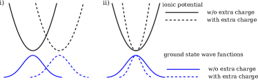
Figure 11: (color online) Sketch of the lattice potential for i) Holstein, and ii) $g_{2}>0$ quadratic models. Full (dashed) lines indicate ionic potential and ground state wavefunction without (with) an extra charge on the site.

Fig. 10 shows that for $g_{2}>0$, $g_{4}=0$, the e-ph coupling has an extremely weak effect even in the atomic limit $t=0$, since the quasiparticle weight $Z$ remains very close to $1$ while the average number of phonons is very small. An explanation for this behaviour is sketched in Fig. 11: in the linear Holstein model, the carrier displaces the harmonic lattice potential of its site, as sketched in the left panel. The overlap between the ground state wavefunctions of the original and the displaced potentials is then the overlap between the tails of two Gaussians with different centers, which decreases exponentially with increasing displacement. Indeed, in the atomic limit for the linear Holstein model $Z\sim\exp[-(g/\Omega)^{2}]$. In the purely quadratic model with positive $g_{2}$, however, the electron merely changes the shape of the well by increasing $\Omega$ to $\Omega_{\text{at}}$. The overlap between the ground states of the original and modified potential is that of two Gaussians with the same center but different widths. We can calculate this overlap analytically to find

$$Z=\sqrt{1-\left(\frac{\Omega-\Omega_{\text{at}}}{\Omega+\Omega_{\text{at}}^{2}}\right)^{2}}$$ (10)

For $\Omega=1.0$, even for $g_{2}=100\Omega$ we still have $Z\approx 0.42$. We conclude that a positive, purely quadratic electron-phonon coupling has negligible effect on the dynamics of a charge carrier. In particular, no crossover into the small polaron regime occurs for positive $g_{2}$ for any reasonable coupling strength. Finite $t$ results (not shown) fully support this conclusion.

References

- (1) H. Matsui, A. S. Mishchenko and T. Hasegawa, Phys. Rev. Lett. 104, 056602 (2010).
- Ciuchi and Fratini (2011) S. Ciuchi and S. Fratini, Physical Review Letters 106, 166403 (2011).
- Lanzara et al. (2001) A. Lanzara, P. V. Bogdanov, X. J. Zhou, S. A. Kellar, D. L. Feng, E. D. Lu, T. Yoshida, H. Eisaki, A. Fujimori, K. Kishio, J.-I. Shimoyama, T. Noda, S. Uchida, Z. Hussain, and Z.-X. Shen, Nature 412, 510 (2001).
- Shen et al. (2004) K. Shen, F. Ronning, D. Lu, W. Lee, N. Ingle, W. Meevasana, F. Baumberger, A. Damascelli, N. Armitage, L. Miller, Y. Kohsaka, M. Azuma, M. Takano, H. Takagi, and Z.-X. Shen, Physical Review Letters 93 (2004), 10.1103/PhysRevLett.93.267002.
- Reznik et al. (2006) D. Reznik, L. Pintschovius, M. Ito, S. Iikubo, M. Sato, H. Goka, M. Fujita, K. Yamada, G. D. Gu, and J. M. Tranquada, Nature 440, 1170 (2006).
- Lee et al. (2006) J. Lee, K. Fujita, K. McElroy, J. A. Slezak, M. Wang, Y. Aiura, H. Bando, M. Ishikado, T. Masui, J.-X. Zhu, A. V. Balatsky, H. Eisaki, S. Uchida, and J. C. Davis, Nature 442, 546 (2006).
- Gadermaier et al. (2010) C. Gadermaier, A. Alexandrov, V. Kabanov, P. Kusar, T. Mertelj, X. Yao, C. Manzoni, D. Brida, G. Cerullo, and D. Mihailovic, Physical Review Letters 105 (2010), 10.1103/PhysRevLett.105.257001.
- Gunnarsson and Rosch (2008) O. Gunnarsson and O. Rösch, Journal of Physics: Condensed Matter 20, 043201 (2008).
- Mannella et al. (2005) N. Mannella, W. L. Yang, X. J. Zhou, H. Zheng, J. F. Mitchell, J. Zaanen, T. P. Devereaux, N. Nagaosa, Z. Hussain, and Z.-X. Shen, Nature 438, 474 (2005).
- Yildirim et al. (2001) T. Yildirim, O. Gülseren, J. Lynn, C. Brown, T. Udovic, Q. Huang, N. Rogado, K. Regan, M. Hayward, J. Slusky, T. He, M. Haas, P. Khalifah, K. Inumaru, and R. Cava, Physical Review Letters 87 (2001), 10.1103/PhysRevLett.87.037001.
- Liu et al. (2001) A. Y. Liu, I. I. Mazin, and J. Kortus, Physical Review Letters 87, 087005 (2001).
- Mazin and Antropov (2003) I. Mazin and V. Antropov, Physica C: Superconductivity 385, 49 (2003).
- Choi et al. (2002) H. J. Choi, D. Roundy, H. Sun, M. L. Cohen, and S. G. Louie, Nature 418, 758 (2002).
- Holstein (1959) T. Holstein, Annals of Physics 8, 325 (1959).
- Fröhlich (1954) H. Fröhlich, Advances in Physics 3, 325 (1954).
- (16) O. Rösch and O. Gunnarson, Phys. Rev. Lett. 92, 146403 (2004); B. Lau, M. Berciu, and G. A. Sawatzky, Phys. Rev. B 76, 174305 (2007); G. L. Goodvin and M. Berciu, Phys. Rev. B 78, 235120 (2008); S. Johnston, F. Vernay, B. Moritz, Z.-X. Shen, N. Nagaosa, J. Zaanen, and T. P. Devereaux, Phys. Rev. B 82, 064513 (2010), and references therein.
- (17) A. Heeger, S. Kivelson, J. R. Schrieffer, and W.-P. Su, Rev. Mod. Phys. 60, 781 (1988).
- (18) S. Barišić, J. Labbé, and J. Friedel, Phys. Rev. Lett. 25, 919 (1970); S. Barišić, Phys. Rev. B 5, 932 (1972); ibid 5, 941 (1972).
- (19) For a small selection of such examples, see Z. Liu and E. Manousakis, Phys. Rev. B 45, 2425 (1992); J. Bala, G. A. Sawatzky, A. M. Oles, and A. Macridin, Phys. Rev. Lett. 87, 067204 (2001); A. S. Mishchenko and N. Nagaosa, Phys. Rev. Lett. 93, 036402 (2004); A. Alvermann, D. M. Edwards, and H. Fehske, Phys. Rev. Lett. 98, 056602 (2007).
- Berciu (2006) M. Berciu, Physical Review Letters 97 (2006).
- Goodvin et al. (2006) G. Goodvin, M. Berciu, and G. Sawatzky, Phys. Rev. B 74 (2006).
- Adolphs and Berciu (2013) C. P. J. Adolphs and M. Berciu, EPL (Europhysics Letters) 102, 47003 (2013).
- Entin-Wohlman et al. (1983) O. Entin-Wohlman, H. Gutfreund, and M. Weger, Solid State Communications 46, 1 (1983).
- Entin-Wohlman et al. (1985) O. Entin-Wohlman, H. Gutfreund, and M. Weger, Journal of Physics C: Solid State Physics 18, L61 (1985).
- Zolotaryuk et al. (1998) Y. Zolotaryuk, P. L. Christiansen, and J. J. Rasmussen, Physical Review B 58, 14305 (1998).
- Raghavan and Kenkre (1994) S. Raghavan and V. M. Kenkre, Journal of Physics: Condensed Matter 6, 10297 (1994).
- Kenkre (1998) V. Kenkre, Physica D: Nonlinear Phenomena 113, 233 (1998).
- Voulgarakis and Tsironis (2000) N. Voulgarakis and G. Tsironis, Physical Review B 63 (2000), 10.1103/PhysRevB.63.014302.
- Maniadis et al. (2003) P. Maniadis, G. Kalosakas, K. Rasmussen, and A. Bishop, Physical Review B 68 (2003), 10.1103/PhysRevB.68.174304.
- Freericks et al. (1993) J. K. Freericks, M. Jarrell, and D. J. Scalapino, Physical Review B 48, 6302 (1993).
- Meyer et al. (2002) D. Meyer, A. Hewson, and R. Bulla, Physical Review Letters 89 (2002), 10.1103/PhysRevLett.89.196401.
- Mitsumoto and Ōno (2005) K. Mitsumoto and Y. Ōno, Physica C: Superconductivity 426–431, Part 1, 330 (2005).
- Bussmann-Holder et al. (1989) A. Bussmann-Holder, A. Simon, and H. Büttner, Physical Review B 39, 207 (1989).
- (34) J. Zaanen, G.A. Sawatzky, and J.W. Allen, Phys. Rev. Lett. 55, 418 (1985).
- (35) O. S. Barišić, Phys. Rev. B. 69, 064302 (2004).
- Möller et al. (2012) M. Möller, A. Mukherjee, C. P. J. Adolphs, D. J. J. Marchand, and M. Berciu, Journal of Physics A: Mathematical and Theoretical 45, 115206 (2012).
- Berciu and Goodvin (2007) M. Berciu and G. L. Goodvin, Physical Review B 76, 165109 (2007).
- (38) O. S. Barišić, Phys. Rev. Lett. 98, 209701 (2007); M. Berciu, Phys. Rev. Lett. 98, 209702 (2007).
- (39) M. Berciu, Can. J. Phys. 86, 523 (2008).