On Landau’s eigenvalue theorem and
information cut-sets

Abstract

A variation of Landau’s eigenvalue theorem describing the phase transition of the eigenvalues of a time-frequency limiting, self adjoint operator is presented. The total number of degrees of freedom of square-integrable, multi-dimensional, bandlimited functions is defined in terms of Kolmogorov’s $n$-width and computed in some limiting regimes where the original theorem cannot be directly applied. Results are used to characterize up to order the total amount of information that can be transported in time and space by multiple-scattered electromagnetic waves, rigorously addressing a question originally posed in the early works of Toraldo di Francia and Gabor. Applications in the context of wireless communication and electromagnetic sensing are discussed.

I Introduction

How much information can a prescribed electromagnetic waveform transport in time and space? This basic question is of mathematical and physical interest, and has numerous engineering applications, including in communications, sensing, imaging, radar detection and classification systems. Information theory of wireless communication provides a partial answer, but assumes a stochastic model of the fading channel, taking for granted the physical nature of the quantities which figure in its formalism. In this paper, we take the point of view that communication of information is the transmission of physical states from transmitters to receivers and, as such, it is subject to the laws of nature. We rigorously compute the physical limits for the transport of information by electromagnetic waves in terms of degrees of freedom, and discuss their significance in an engineering context.

Our results build upon Landau’s theorem [1], concerning the asymptotic behavior of the eigenvalues of a certain integral equation arising from the problem of simultaneous concentration of a function and its Fourier transform. This theorem asserts that, in a well defined sense, the eigenvalues undergo a sharp transition from values close to one to values close to zero, and the scale of this transition characterizes the asymptotic dimension of the space of bandlimited functions. The problem was originally considered jointly by Landau, Pollak and Slepian in a series of papers [2, 3, 4, 5, 6], of which [7] and [8] provide excellent tutorial reviews. The precise width of the transition in the single-dimensional case has been first conjectured by Slepian [9], and finally computed rigorously by Landau and Widom [10]. The theorem we refer here gives only the first order characterization of the transition, but it describes concentration over arbitrary sets and in arbitrary dimensions. We provide extensions of the original statement, and apply them in certain geometric configurations arising in the context of information transport through electromagnetic propagation.

Consider a wireless network in which a set of users located in one region of the network wishes to communicate with users located in an another region, see Figure 1. The number of channels available for communication is limited by the dimensionality of the signal’s space on the cut-set boundary through which electromagnetic propagation occurs.

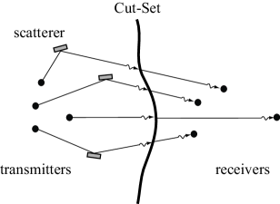
Figure 1: Parallel channels consume spatial resource along the cut.

This corresponds to the minimum number of basis functions required to represent the signal on the cut-set boundary, and is independent of the communication scheme employed. It provides a bound on the amount of spatial and frequency multiplexing achievable using arbitrary technologies and in arbitrary scattering environments. It essentially corresponds to the number of degrees of freedom of the space-time field used for communication and is determined by the phase transition of the eigenvalues referred above. Similarly, the number of independent features that can be extracted from a scattering system using a probe signal for remote sensing, imaging, detection and classification systems is limited by the number of degrees of freedom of the field and characterized by the same phase transition.

We compute the number of degrees of freedom of multiple scattered electromagnetic waves in terms of Kolmogorov’s $n$-width, and provide a physical interpretation in terms of cut-set information flow. Our results extend the single frequency treatments of  [11, 12, 13, 14, 15, 16, 17, 18] to signals of non-zero frequency bandwidth. In a broader framework, they rigorously address the question of how much information does an electromagnetic waveform carry in time and space, first posed in the early works of Toraldo di Francia [19, 20] and Gabor [21, 22].

The number of degrees of freedom of the field is also related to the information capacity of multi-user communication systems. Its application to bound the Shannon capacity scaling of wireless networks is described in [17] and [18], and can be extended to signals with a non-zero frequency band using the results given here.

The rest of the paper is organized as follows. The next section provides rigorous statements of the mathematical results. Applications are discussed in Section III. Section IV draws conclusions and mentions some possible future work. The proof of the main theorem is given in Appendix -A.

II Statement of the results

We begin by presenting our results in two dimensions, as this form better suits the application discussed in the next section. A more general statement appears at the end of this section. Let $P$ and $Q$ be measurable sets in $\mathbb{R}^{2}$ with boundaries of measure zero. For any point $\textbf{p}\in\mathbb{R}^{2}$, and positive scalar $\beta>0$, we indicate by $\beta(P+\textbf{p})$ the set of points of the form $\beta({\bf{x}}+\textbf{p})$ with ${\bf{x}}\in P$. Clearly, we have

$$m(\beta P)=\beta^{2}m(P),$$ (1)

where $m(\cdot)$ indicates Lebesgue measure. Similarly, for ${\bf{x}}=(x_{1},x_{2})$, we have

$$m\{(\beta x_{1},x_{2}):{\bf{x}}\in P\}=\beta\,m(P).$$ (2)

For any two points ${\bf{x}}=(x_{1},x_{2})$, ${\bf{u}}=(u_{1},u_{2})$, we let ${\bf{x}}\cdot{\bf{u}}=x_{1}u_{1}+x_{2}u_{2}$. For $f\in L^{2}(\mathbb{R}^{2})$, the Fourier transform of $f$ is

$$\mathcal{F}f=\int_{\mathbb{R}^{2}}f({\bf{x}})\exp(-i{\bf{x}}\cdot{\bf{u}})d{\bf{x}}.$$ (3)

Consider now two subspaces of $L^{2}(\mathbb{R}^{2})$ consisting of the functions supported in $P$ and of those whose Fourier transform is supported in $Q$, namely

$$\mathscr{T}_{P} =\{f\in L^{2}:f({\bf{x}})=0,\;{\bf{x}}\not\in P\},$$ (4)

$$\mathscr{B}_{Q} =\{f\in L^{2}:\mathcal{F}f({\bf{u}})=0,\;{\bf{u}}\not\in Q\}.$$ (5)

The orthogonal projections onto these subspaces are defined using the indicator function

$$\mathds{1}_{Q}({\bf{x}})=\left\{\begin{array}[]{ll}1&\mbox{if ${\bf{x}}\in Q$},\\ 0&\mbox{otherwise},\end{array}\right.$$ (6)

in the following way

$$\mathcal{T}_{P}f =\mathds{1}_{P}({\bf{x}})f({\bf{x}}),$$ (7)

$$\mathcal{B}_{Q}f =\mathcal{F}^{-1}\mathds{1}_{Q}\mathcal{F}f=\int_{\mathbb{R}^{2}}h({\bf{x}}-{\bf{y}})f({\bf{y}})d{\bf{y}},$$ (8)

where

$$\mathcal{F}h=\mathds{1}_{Q}.$$ (9)

We are interested in the behavior of the eigenvalues in the integral equation

$$\mathcal{T}_{P}\mathcal{B}_{Q}\mathcal{T}_{P}\varphi({\bf{x}})=\lambda\varphi({\bf{x}}),$$ (10)

where the operator $\mathcal{T}_{P}\mathcal{B}_{Q}\mathcal{T}_{P}$ is positive, self-adjoint, compact, and bounded by one. The eigenvalues are a countable set that characterizes the asymptotic dimension of the subspace $\mathscr{B}_{Q}$. Namely, the number of eigenvalues above level $\epsilon$ corresponds to the dimension of the minimal subspace approximating the elements of $\mathscr{B}_{Q}$ within $\epsilon$ accuracy over the set $P$. A rigorous definition of asymptotic dimension is given in Section III. To determine this number, Landau [1] considered the case where $Q$ is a fixed set, while $P$ varies over the family $\beta P^{\prime}$, with $P^{\prime}$ fixed, and determined the number of eigenvalues significantly greater than zero as $\beta\rightarrow\infty$. It turns out that the eigenvalues arranged in non-increasing order undergo a transition from values close to one to values close to zero in an interval of indexes around $\beta^{2}$. The transition is sharp, of width $o(\beta^{2})$, so that the eigenvalues plotted as a function of their indexes appear as a step function when viewed at the scale of $\beta^{2}$, see Figure 2.

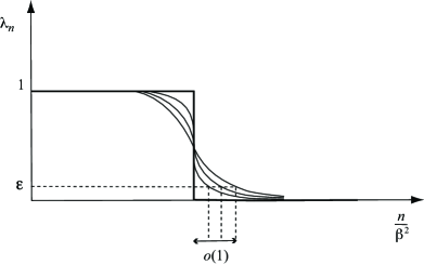
Figure 2: Phase transition of the eigenvalues.

The asymptotic dimension of the space $\mathscr{B}_{Q}$ is given by the transition point of this step function, that is of the order of $\beta^{2}$, when the support set $P$ is appropriately scaled by blowing-up all of its coordinates. Due to symmetry, the asymptotic dimension of the space $\mathscr{T}_{P}$ can similarly be obtained by considering the operator $\mathcal{B}_{Q}\mathcal{T}_{P}\mathcal{B}_{Q}$ and scaling $Q=\beta Q^{\prime}$ while keeping $P$ fixed. The precise result is stated as follows:

Theorem 1.

(Landau). For any $0<\epsilon<1$, let $N_{\beta}(\epsilon)$ be the number of eigenvalues of $\mathcal{T}_{\beta P^{\prime}}\mathcal{B}_{Q}\mathcal{T}_{\beta P^{\prime}}$ not smaller than $\epsilon$, then we have

$$\lim_{\beta\rightarrow\infty}\frac{N_{\beta}(\epsilon)}{\beta^{2}}=(2\pi)^{-2}m(P^{\prime})m(Q).$$ (11)

In Landau’s case, spectral concentration is achieved by scaling all coordinates of one of the two support sets. We prove the analogous result by scaling only one coordinate of both support sets. While in Landau’s case the scaling of the coordinates is uniform, in our case coordinates are scaled at independent rates.

Let $P$ and $Q$ be two fixed sets. We consider the following families

$$P_{\tau}=\{(\tau x_{1},x_{2}):(x_{1},x_{2})\in P\}$$ (12)

$$Q_{\rho}=\{(x_{1},\rho x_{2}):(x_{1},x_{2})\in Q\}.$$ (13)

Theorem 2.

For any $0<\epsilon<1$, let $N_{\tau,\rho}(\epsilon)$ be the number of eigenvalues of $\mathcal{T}_{P_{\tau}}\mathcal{B}_{Q_{\rho}}\mathcal{T}_{P_{\tau}}$ not smaller than $\epsilon$, then we have

$$N_{\tau,\rho}(\epsilon)=(2\pi)^{-2}m(P)m(Q)\tau\rho+o(\tau\rho),$$ (14)

as $\tau,\rho\rightarrow\infty$.

The proof is based on decomposing the operator using orthonormal functions, and then computing an integral that differs from the one of Landau, due to the different scaling of the space. The result also extends to higher dimensions, where any combination of coordinates’ scaling in the original or transformed domain can be performed. Our theorem can be stated for any invertible linear mapping of the support sets, subject to a limiting condition. Let $P$ and $Q$ be measurable sets in $\mathbb{R}^{N}$ with boundaries of measure zero. For any real matrix ${\mathrm{A}}$ of size $N\times N$, we indicate by ${\mathrm{A}}P$ the set of points of the form ${\mathrm{A}}{\mathrm{x}}$, where ${\mathrm{x}}$ is the column vector composed of the elements of ${\bf{x}}\in P$. We also indicate with $|{\mathrm{A}}|$ the determinant of ${\mathrm{A}}$, with ${\mathrm{A^{T}}}$ the transpose of ${\mathrm{A}}$, and with with $U$ the unit ball in $L^{2}(\mathbb{R}^{N}).$ We let ${\mathrm{A}}={\mathrm{A}}(\tau)$ and ${\mathrm{B}}={\mathrm{B}}(\rho)$ for real parameters $\tau$ and $\rho$. The case in which either matrix is constant, or depends on multiple parameters is completely analogous.

Theorem 3.

For any $0<\epsilon<1$, let $N_{{\mathrm{A}},{\mathrm{B}}}(\epsilon)$ be the number of eigenvalues of $\mathcal{T}_{{\mathrm{A}}P}\mathcal{B}_{{\mathrm{B}}Q}\mathcal{T}_{{\mathrm{A}}P}$ not smaller than $\epsilon$. If

$$\lim_{(\tau,\rho)\rightarrow(\tau_{0},\rho_{0})}{\mathrm{B^{T}}}{\mathrm{A}}U=\mathbb{R}^{N},$$ (15)

then we have

$$\lim_{(\tau,\rho)\rightarrow(\tau_{0},\rho_{0})}\frac{N_{{\mathrm{A}},{\mathrm{B}}}(\epsilon)}{|{\mathrm{A}}|\,|{\mathrm{B}}|}=(2\pi)^{-N}m(P)m(Q).$$ (16)

Landau’s theorem is a special case where ${\mathrm{A}}$ is a scalar matrix and ${\mathrm{B}}$ is the identity. Its two-dimensional version is stated in Theorem 1. Theorem 2 corresponds to the special case

$${\mathrm{A}}=\left(\begin{array}[]{cc}\tau&0\\ 0&1\end{array}\right)\;\;{\mathrm{B}}=\left(\begin{array}[]{cc}1&0\\ 0&\rho\end{array}\right).$$ (17)

III Application of the results

Landau [1] does not mention the extensions to his theorem described above, but no doubt that if asked he could have proved them effortlessly. Nonetheless, these results do not seem to appear anywhere. We believe that our main contribution is to point out their significance in the context of communication and sensing using electromagnetic waves.

III-A The number of degrees of freedom

When communication occurs through propagation of electromagnetic waves, the effective dimensionality, or number of degrees of freedom, of the space-time field is a key information-theoretic quantity related to the capacity of any spatially distributed communication system [17, 18]. This quantity can be computed by evaluating the number of significant eigenvalues in Theorems 1, 2, or 16.

Consider the space $\mathscr{S}$ of real space-time waveforms $f(s,t)\in L^{2}(\mathbb{R}^{2})$ and equipped with the norm

$$||f||^{2}=\left(\iint_{P}f^{2}(s,t)dsdt\right)^{1/2}.$$ (18)

A subspace $\mathscr{B}_{Q}\subset\mathscr{S}$ is given by the space of functions $f(s,t)\in L^{2}(\mathbb{R}^{2})$ of spectral support $Q$. We assume their energy is normalized so that

$$\iint_{\mathbb{R}^{2}}f^{2}(s,t)dsdt\leq 1.$$ (19)

Given a level of accuracy $\epsilon>0$, define the number of degrees of freedom at level $\epsilon$ of the space $\mathscr{B}_{Q}$ in $\mathscr{S}$

$$\mathcal{N}_{\epsilon}(\mathscr{B}_{Q})=\min\{n:d_{n}(\mathscr{B}_{Q},\mathscr{S})\leq\epsilon\},$$ (20)

where $d_{n}(\mathscr{B}_{Q},\mathscr{S})$ is the Kolmogorov $n$-width [23] of the space $\mathscr{B}_{Q}$ in $\mathscr{S}$. Letting $\mathscr{S}_{n}$ be an $n$-dimensional subspace of $\mathscr{S}$, this is defined as

$$d_{n}(\mathscr{B}_{Q},\mathscr{S})=\inf_{\mathscr{S}_{n}\subset\mathscr{S}}D_{\mathscr{S}_{n}}(\mathscr{B}_{Q}),$$ (21)

where the deviation

$$D_{\mathscr{S}_{n}}(\mathscr{B}_{Q})=\sup_{f\in\mathscr{B}_{Q}}\inf_{g\in\mathscr{S}_{n}}||f-g||.$$ (22)

In words, the deviation represents how well $\mathscr{B}_{Q}$ may be uniformly approximated by the elements of an $n$-dimensional subspace of $\mathscr{S}$, while the $n$-width is the smallest of such deviations over all $n$-dimensional subspaces of $\mathscr{S}$. The number of degrees of freedom $N_{\epsilon}(\mathscr{B}_{Q})$ represents the dimension of the minimal subspace representing the elements of $\mathscr{B}_{Q}$ within $\epsilon$ accuracy over the set $P$. A basic result in approximation theory (see e.g. [23, Ch. 2, Prop. 2.8]) states that

$$d_{n}(\mathscr{B}_{Q},\mathscr{S})=\sqrt{\lambda_{n}},$$ (23)

where $\lambda_{n}$ is the $n$-th eigenvalue (arranged in non-increasing order) of the Fredholm integral equation of the second kind in (10). It now follows from (23) that Theorem 2 allows to compute the number of degrees of freedom by scaling only one of the two coordinates of the space-time field, together with the transformed version of the other.

The number of degrees of freedom defined in this way appears to be a principal feature of the mathematical model of the real world of transmitted signals, that is practically insensitive to small changes of a secondary feature of the model, such as the accuracy $\epsilon$ of the measurement apparatus with which the signals are detected. This is evident by rewriting (14) as

$$N_{\tau,\rho}(\epsilon)=(2\pi)^{-2}m(P)m(Q)\,\tau\rho+o(\tau\rho)\;\;\;\mbox{as }\tau,\rho\rightarrow\infty,$$ (24)

where the $\epsilon$-dependence appears hidden as a pre-constant of the second order term $o(\tau\rho)$ in the phase transition of the eigenvalues.

III-B Cut-set of two-dimensional circular domains

Theorems 1 and 2 can be applied to evaluate the number of degrees of freedom of waveforms of a given frequency band over spatial cut-sets separating transmitters and receivers in a wireless communication setting, or separating scattering objects from sensing devices in imaging and sensing systems.

Consider the case of a two-dimensional domain of cylindrical symmetry,

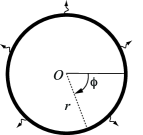
Figure 3: Cut-set boundary of two-dimensional circular domain.

in which an electromagnetic field is radiated by a configuration of currents located inside a circular domain of radius $r$ of an arbitrary scattering environment, oriented perpendicular to the domain, and constant along the direction of flow. This can model, for example, an arbitrary scattering environment where a spatial distribution of wireless transmitters is placed inside the circular domain, and communicate to receivers placed outside the domain. The same model applies to a remote sensing system where objects inside the domain are illuminated by an external waveform, and the scattered field is recovered by sensors placed outside the domain. The radiated field away from the scattering system and measured at the receivers is completely determined by the field on the cut-set boundary through which it propagates, see Figure 3. On this boundary, we can refer to a scalar field $f(\phi,t)$ that is a function of only two scalar variables: one angular and one temporal. The corresponding four field’s representations, linked by Fourier transforms, are depicted in Figure 4, where the angular frequency $\omega$ indicates the transformed coordinate of the time variable $t$, the wavenumber $w$ indicates the transformed coordinate of the angular variable $\phi$, and $\mathcal{F}f(\phi,t)=\widehat{F}(w,\omega)$.

Figure 4: Field’s representations linked by Fourier transforms.

For convenience, we let $r$ be normalized by the speed of light, so that both radius-frequency and time-frequency products are dimensionless quantities. We wish to determine the number of degrees of freedom of the space-time field $f(\phi,t)$ on the cut-set boundary, that is radiated for $t\in[-T/2,T/2]$ and occupies a bandwidth $\omega\in[-\Omega,\Omega]$; it is observed over the interval $\phi\in[-\pi,\pi]$ and occupies a wavenumber bandwidth $w\in[-W,W]$. Of course, these statements make little mathematical sense since a field satisfying above constraints would have bounded support in both the natural and transformed domain, so it would be zero everywhere. To make our considerations precise, we need to take appropriate scaling limits.

To determine the correct scaling laws for the support sets of the field, we introduce some geometric constraints. On the one hand, we limit the observation domain to $\phi\in[-\pi,\pi]$, so that the spatially periodic field on the cut-set boundary is observed over a single period. On the other hand, it is well known [11] that in this case the wavenumber bandwidth is related to the frequency of transmission in such a way that for any possible configuration of sources and scatterers inside the circular radiating domain, we have at most

$$w=\omega r+o(\omega r)\;\;\;\mbox{as }\omega r\rightarrow\infty.$$ (25)

It follows that we need to scale the support sets of the field subject to the constraints depicted in Figure 5.

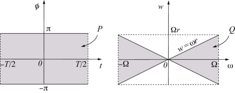
Figure 5: Support sets in the natural and transformed domains.

We can blow-up the spectral support $Q$ while keeping $P$ fixed by letting $\Omega\rightarrow\infty$. In this case, by Theorem 1 the number of degrees of freedom over a fixed transmission time and cut-set interval of width $2\pi$, in the wide band frequency regime is

$$\mathcal{N}_{\epsilon}(\mathscr{B}_{Q}) =\frac{2\Omega^{2}rT2\pi}{(2\pi)^{2}}+o(\Omega^{2})$$

$$=\frac{\Omega T}{\pi}\frac{2\pi r\Omega}{2\pi}+o(\Omega^{2})\;\;\;\mbox{as }\Omega\rightarrow\infty.$$ (26)

On the other hand, our geometric configuration does not allow to blow-up the support $P$ while keeping $Q$ fixed because the cut-set domain is limited to an angle $2\pi$. Landau’s theorem in its original form is of no help here, but we can apply Theorem 2 to obtain the number of degrees of freedom over a fixed frequency band, by scaling the time coordinate of $P$ and the coordinate of $Q$ corresponding to the size of the radiating system, and we have

$$\mathcal{N}_{\epsilon}(\mathscr{B}_{Q}) =\frac{\Omega T}{\pi}\frac{2\pi r\Omega}{2\pi}+o(rT)\;\;\;\mbox{as }T,r\rightarrow\infty.$$ (27)

Equations (26) and (27) show that the number of degrees of freedom is given by the product of two factors, each viewed in an appropriate asymptotic regime: one accounting for the number of degrees of freedom in the time-frequency domain, $\Omega T/\pi$, and another accounting for the number of degrees of freedom in the space-wavenumber domain, $2\pi r\Omega/(2\pi)$. The latter factor physically corresponds to the perimeter of the disc of radius $r$ normalized by an interval of wavelengths $2\pi/\Omega$, and can be interpreted as the spatial cut-set through which the information must flow. The idea is that for any finite size system, the wavenumber bandwidth is a limited resource. Each parallel channel occupies a certain amount of spatial resource on the cut, proportional to the wavelength of transmission, and these channels must be sufficiently spaced along the cut for the corresponding waveforms to provide independent streams of information. The total number of channels is then given by the total spatial resource, given by the cut-length $2\pi r$, divided by the total occupation cost, given by the wavelength-interval $2\pi/\Omega$.

III-C Comparison with the single-dimensional case

The number of time-frequency degrees of freedom of any signal $f(t)\in L^{2}(\mathbb{R})$ bandlimited to $[-\Omega,\Omega]$, or timelimited to $[-T/2,T/2]$, is given by the time-bandwidth product

$$\mathcal{N}_{\epsilon}(\mathscr{B}_{\Omega})=\frac{\Omega T}{\pi}+o(\Omega T)\;\;\;\mbox{as }\Omega T\rightarrow\infty.$$ (28)

In this case, spectral concentration occurs by scaling either the transmission time $T$, or the frequency band $\Omega$. The work in [10] gives the precise asymptotic order of the term $o(\Omega T)$, which is $\log(\Omega T)\log(1/\epsilon)$.

Similarly, letting $W=\omega r+o(\omega r)$, the number of space-wavenumber degrees of freedom of any signal $f(\phi)\in L^{2}[-\pi,\pi]$ radiated with frequency $\omega$ from the interior of a circular domain of radius $r$ and observed on the circular perimeter boundary of angle $\phi\in[-\pi,\pi]$, is given by the space-bandwidth product

$$\mathcal{N}_{\epsilon}(\mathscr{T}_{2\pi})=\frac{\omega 2\pi r}{\pi}+o(\omega r)\;\;\;\mbox{as }r\omega\rightarrow\infty.$$ (29)

In this case, spectral concentration occurs by scaling either the size of the radiating system $r$, or the frequency of transmission $\omega$.

The results (26) and (27) can be viewed as a combination of (28) and (29). An heuristic way to compute the total number of degrees of freedom of the space-time field $f(t,\phi)$ would be to integrate over frequencies while accounting for the number of spatial degrees of freedom that every frequency component carries. This corresponds to simply integrate (29) over the frequency bandwidth and, according to (28), multiply the result by $T/\pi$

$$\mathcal{N}_{\epsilon}(\mathscr{B}_{Q}) =\frac{T}{\pi}\int_{0}^{\Omega}\frac{\omega 2\pi r}{\pi}d\omega,$$

$$=\frac{\Omega T}{\pi}\frac{2\pi r\Omega}{2\pi},$$ (30)

which gives the correct result. Of course, the problem of this heuristic is clear: it does not account for the possible accumulation of the error $\epsilon$ when computing the integral along the frequency spectrum. Thus, the need for the rigorous method presented in this paper arises.

III-D Cut-set of three-dimensional spherical domains

We extend results to three dimensions by considering a spherical radiating system of radius $r$. In this case, the surface of the sphere is interpreted as a cut-set through which the information must flow and provides a limit on the amount of information that can radiate from the interior of the domain to the outside space. Each scalar component $f(\phi_{1},\phi_{2},t)$ of the vector field on the cut-set boundary is a function of two angular coordinates identifying a point on the surface and one temporal one, see Figure 6.

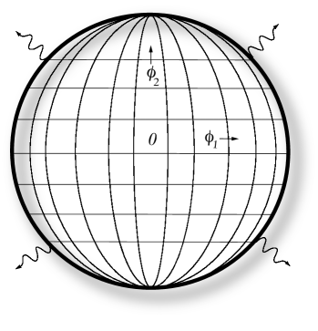
Figure 6: Cut-set boundary of three-dimensional spherical domain.

The support sets of each scalar field component are the ones depicted in Figure 7, where we indicate with $w_{1}$ the transformed coordinate of the variable $\phi_{1}$, with $w_{2}$ the transformed coordinate of the variable $\phi_{2}$, and with $\Phi$ the solid angle subtended by the surface boundary at the center of the sphere.

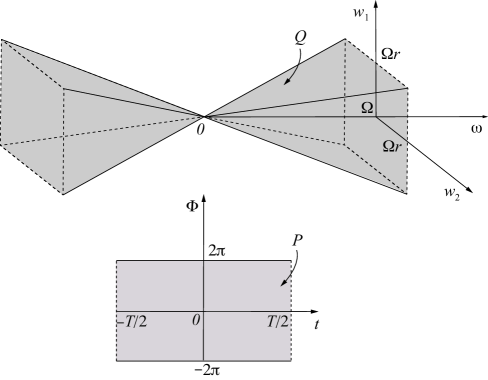
Figure 7: Support sets in the natural and transformed domains.

We then have

$$m(P)=4\pi T,$$ (31)

$$m(Q)=\frac{8}{3}\Omega^{3}r^{2}.$$ (32)

By Theorem 16, with Landau’s type scaling

$${\mathrm{A}}=\left(\begin{array}[]{ccc}1&0&0\\ 0&1&0\\ 0&0&1\end{array}\right),\;\;{\mathrm{B}}=\left(\begin{array}[]{ccc}\rho&0&0\\ 0&\rho&0\\ 0&0&\rho\end{array}\right),$$ (33)

and using (31) and (32), it follows that the number of degrees of freedom in the wide band frequency regime is

$$\mathcal{N}_{\epsilon}(\mathscr{B}_{Q})=4\pi r^{2}\frac{\Omega^{3}T}{3\pi^{3}}+o(\Omega^{3})\;\;\;\mbox{as }\Omega\rightarrow\infty,$$ (34)

where $\Omega=\rho\Omega^{\prime}$ with $\Omega^{\prime}$ fixed and $\rho\rightarrow\infty$. With the alternative scaling

$${\mathrm{A}}=\left(\begin{array}[]{ccc}\tau&0&0\\ 0&1&0\\ 0&0&1\end{array}\right),\;\;{\mathrm{B}}=\left(\begin{array}[]{ccc}1&0&0\\ 0&\rho&0\\ 0&0&\rho\end{array}\right),$$ (35)

we also have that the number of degrees of freedom over a fixed frequency band for large radiating systems and transmission time is

$$\mathcal{N}_{\epsilon}(\mathscr{B}_{Q})=4\pi r^{2}\frac{\Omega^{3}T}{3\pi^{3}}+o(r^{2}T)\;\;\;\mbox{as }T,r\rightarrow\infty,$$ (36)

where $T=\tau T^{\prime}$, $r=\rho r^{\prime}$, with $T^{\prime},r^{\prime}$ fixed and $\tau,\rho\rightarrow\infty$.

Above rigorous results can also be obtained using the heuristic method described in Section III-C. The number of space-wavenumber degrees of freedom of the electromagnetic field radiated with frequency $\omega$ from the interior of a spherical domain of radius $r$ and observed on the surface boundary of solid angle $\Phi\in[-2\pi,2\pi]$, is given by the space-bandwidth product [11, 12]

$$\mathcal{N}_{\epsilon}(\mathscr{T}_{4\pi})=\frac{\omega^{2}4\pi r^{2}}{\pi^{2}}+o[(\omega r)^{2}]\;\;\;\mbox{as }r\omega\rightarrow\infty.$$ (37)

Integrating over the frequency bandwidth and multiplying the result by $T/\pi$, we obtain

$$\mathcal{N}_{\epsilon}(\mathscr{B}_{Q}) =\frac{4\pi r^{2}}{\pi^{2}}\frac{T}{\pi}\int_{0}^{\Omega}\omega^{2}d\omega$$

$$=4\pi r^{2}\frac{\Omega^{3}T}{3\pi^{3}},$$ (38)

which is consistent with the rigorous results in (34) and (36).

III-E Cut-set of general rotationally symmetric domains

Results can be further generalized considering a radiating system enclosed in a convex domain bounded by a surface with rotational symmetry. Consider a cylindrical coordinate system $(r,\phi,z)$, a closed analytic curve $\zeta=\zeta(r,z)$ lying in the plane $\phi=0$ and symmetric with respect to the $z$ axis, and the surface of revolution obtained by rotating the curve about the $z$ axis, see Figure 8.

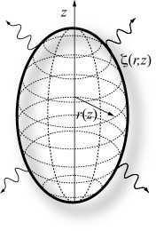
Figure 8: Cut-set boundary of three-dimensional rotationally symmetric domain.

In this case, we can choose a pair of coordinates $(\phi_{1},\phi_{2})$ on the surface such that any meridian curve covers a $2\pi$ range, and the spatial bandwidth along the meridian is constant and bounded by [26]

$$w_{1}=\omega\frac{\ell}{2\pi}+o(\omega\ell)\;\;\mbox{as }\omega\ell\rightarrow\infty,$$ (39)

where $\ell$ is the Euclidean length of the curve, normalized to the speed of light so that $\omega\ell$ is dimensionless. This should be compared with the geometric constraint for circular curves given in (25). On the other hand, any latitude line is a circle of radius $r(z)$ that also covers a $2\pi$ range, and the spatial bandwidth along this line is bounded by

$$w_{2}=\omega r(z)+o(\omega r),\;\;\mbox{as }\omega r\rightarrow\infty.$$ (40)

It follows that while the domain $P$ covers a solid angle $4\pi$, the domain $Q$ varies along $z$ according to the meridian curve parametrization $\zeta=\zeta(r,z)$, and we have

$$m(P)=4\pi T,$$ (41)

$$m(Q) =\frac{8\Omega^{3}}{3}\ \frac{\ell}{2\pi}\frac{\pi}{2}\int_{\zeta}r(z)dz$$

$$=\frac{8\Omega^{3}}{3}\frac{\ell}{4\pi}\int_{\zeta}\pi r(z)dz$$

$$=\frac{8\Omega^{3}}{3}\frac{\mathcal{A}}{4\pi},$$ (42)

where $\mathcal{A}$ is the surface area of the radiating volume.

By Theorem 16, the scaling in (33), and using (41) and (42), we have that the number of degrees of freedom in the wide band frequency regime is

$$\mathcal{N}_{\epsilon}(\mathscr{B}_{Q})=\frac{\mathcal{A}\Omega^{3}T}{3\pi^{3}}+o(\Omega^{3})\;\;\;\mbox{as }\Omega\rightarrow\infty,$$ (43)

where $\Omega=\rho\Omega^{\prime}$ with $\Omega^{\prime}$ fixed and $\rho\rightarrow\infty$. The analogous result is obtained by letting the transmission time $T=\tau T^{\prime}$, with $T^{\prime}$ fixed and $\tau\rightarrow\infty$, and blowing-up all coordinates of the radiating volume, so that both $\ell=\rho\ell^{\prime}$ and $r=\rho r^{\prime}(z)$ tend to infinity with $\ell^{\prime}$ and $r^{\prime}$ fixed and $\rho\rightarrow\infty$. In this case, by Theorem 16 with the scaling in (35), and using (41) and (42), we have

$$\mathcal{N}_{\epsilon}(\mathscr{B}_{Q})=\frac{\mathcal{A}\Omega^{3}T}{3\pi^{3}}+o(\mathcal{A}T)\;\;\;\mbox{as }T,\mathcal{A}\rightarrow\infty,$$ (44)

where $\mathcal{A}=\rho^{2}\mathcal{A^{\prime}}$, with $\mathcal{A}^{\prime}$ fixed and $\rho\rightarrow\infty$. Finally, we can check that the result is consistent with the heuristic calculation: starting with the number of space-wavenumber degrees of freedom per angular frequency $\omega$ [18, 26]

$$\mathcal{N}_{\epsilon}(\mathscr{T}_{4\pi})=\frac{\mathcal{A}\omega^{2}}{\pi^{2}},$$ (45)

integrating over the frequency bandwidth and multiplying by $T/\pi$, the result follows.

III-F Degrees of freedom of modulated signals

The results can be extended to handle the case of modulated signals. Consider the case of a real signal modulating a sinusoid of carrier frequency $\omega_{c}$, occupying a bandwidth $\Delta\omega=[\omega_{1},\omega_{2}]$ centered around $\omega_{c}$, see Figure 9.

Figure 9: Support set of a modulated signal in the transformed domain.

In the two-dimensional case, following the same procedure of the previous sections, letting $T=\tau T^{\prime}$, $r=\rho r^{\prime}$, and $\rho,\tau\rightarrow\infty$, we obtain

$$\mathcal{N}_{\epsilon}(\mathscr{B}_{Q}) =\frac{T}{\pi}\frac{2\pi r}{\pi}\frac{(\omega_{2}^{2}-\omega_{1}^{2})}{2}+o(rT)$$

$$=\frac{T\Delta\omega}{\pi}\frac{2\pi r\omega_{c}}{\pi}+o(rT),$$ (46)

as $r,T\rightarrow\infty.$

On the other hand, letting $\Delta\omega=\rho\Delta\omega^{\prime}$, $\omega_{c}=\rho\omega_{c}^{\prime}$, and $\rho\rightarrow\infty$, we have

$$\mathcal{N}_{\epsilon}(\mathscr{B}_{Q})=\frac{T\Delta\omega}{\pi}\frac{2\pi r\omega_{c}}{\pi}+o(\omega_{c}\Delta\omega),$$ (47)

as $\omega_{c},\Delta\omega\rightarrow\infty$. The number of degrees of freedom is proportional to the time-bandwidth product and to the cut-set boundary normalized by the radiating carrier.

For spherical domains, letting $T=\tau T^{\prime}$, $r=\rho r^{\prime}$, and $\tau,\rho\rightarrow\infty$, we have

$$\mathcal{N}_{\epsilon}(\mathscr{B}_{Q}) =\frac{T}{\pi}\frac{4\pi r^{2}}{\pi^{2}}\frac{(\omega_{2}^{3}-\omega_{1}^{3})}{3}+o(Tr^{2})$$

$$=\frac{T\Delta\omega}{\pi}\frac{4\pi r^{2}}{\pi^{2}}\frac{(\omega_{2}^{2}+\omega_{1}^{2}+\omega_{1}\omega_{2})}{3}+o(Tr^{2})$$

$$=\frac{T\Delta\omega}{\pi}\frac{4\pi r^{2}\omega_{c}^{2}}{\pi^{2}}(1+\delta)+o(Tr^{2}),$$ (48)

as $T,r\rightarrow\infty$, where $\delta$ is a constant that depends only on the ratio $\Delta\omega/\omega_{c}$. Analogously, letting $\Delta\omega=\rho\Delta\omega^{\prime}$, $\omega_{c}=\rho\omega_{c}^{\prime}$, $\rho\rightarrow\infty$, we have

$$\mathcal{N}_{\epsilon}(\mathscr{B}_{Q}) =\frac{T\Delta\omega}{\pi}\frac{4\pi r^{2}\omega_{c}^{2}}{\pi^{2}}(1+\delta)+o(\omega_{c}^{2}\Delta\omega),$$ (49)

as $\omega_{c},\Delta\omega\rightarrow\infty$.

Results (48) and (49) can also be combined using the scaling matrices

$${\mathrm{A}}=\left(\begin{array}[]{ccc}\tau&0&0\\ 0&1&0\\ 0&0&1\end{array}\right),\;\;{\mathrm{B}}=\left(\begin{array}[]{ccc}\beta&0&0\\ 0&\rho\beta&0\\ 0&0&\rho\beta\end{array}\right),$$ (50)

and letting $\tau\beta,\rho\beta\rightarrow\infty$, obtaining

$$\mathcal{N}_{\epsilon}(\mathscr{B}_{Q}) =\frac{T\Delta\omega}{\pi}\frac{4\pi r^{2}\omega_{c}^{2}}{\pi^{2}}(1+\delta)+o(r^{2}\omega_{c}^{2}\Delta\omega T),$$ (51)

as $r\omega_{c},\Delta\omega T\rightarrow\infty$.

Finally, for general rotationally symmetric domains, using (50) we have

$$\mathcal{N}_{\epsilon}(\mathscr{B}_{Q})=\frac{T\Delta\omega}{\pi}\frac{\mathcal{A}\omega_{c}^{2}}{\pi^{2}}(1+\delta)+o(\mathcal{A}\omega_{c}^{2}\Delta\omega T),$$ (52)

as $\mathcal{A}\omega_{c}^{2},\Delta\omega T\rightarrow\infty$, where $\mathcal{A}=\rho^{2}\mathcal{A}^{\prime}$ with $\mathcal{A}^{\prime}$ fixed.

For narrowband signals $\Delta\omega/\omega_{c}\ll 1$, and the constant $\delta$ can be made arbitrarily small, so that the number of degrees of freedom in three dimensions is essentially given by the first term of (52), which is the natural extension of of the single-frequency result in [18, 26] and reported in (45), accounting for a non-zero frequency band around frequency $\pm\omega_{c}$. It follows that the number of degrees of freedom per unit time and per unit frequency band is essentially given by

$$N_{0}=\frac{\mathcal{A}\omega_{c}^{2}}{\pi^{2}}.$$ (53)

IV Concluding remarks

A key insight of our analysis is that the amount of information, in terms of degrees of freedom, scales with the surface boundary, rather than with the volume of the space. Clearly, field theory allows for a much larger number of possible field configurations inside the radiating volume. Think for example of the number of standing waves insides a black body. This grows with the volume of the space rather than with the surface area. Our results apply to the information that one can gather about these volumetric configurations, from the point of view of an external observer, through electromagnetic propagation. They pose an information-theoretic limit in terms of degrees of freedom at the scale of the surface boundary through which the field propagates. Physically, this is due to the Green’s propagation operator relating source currents to the radiated field, that essentially behaves as a spatial filter, projecting the number of observable field configurations onto a lower dimensional space [11]. The resulting wavenumber bandlimitation of the field dictates the geometric constraints on the support sets depicted in Figures 5, 7, and 9, leading to our results. The conclusion is that Nature “hides” three-dimensional field configurations, and the world appears to an external observer as having only an apparent three-dimensional informational structure, subject to a two-dimensional representation. Like for Plato’s prisoners in the cave, “the truth would be literally nothing but the shadows of the images.”

Another important observation is that for any fixed size system the amount of information scales with the radiated frequency. We can increase the number of degrees of freedom as high as we want by transmitting signals modulating larger and larger frequencies. In wireless networks, this has been used to identify regimes of linear capacity scaling with the number of users [24, 25]. In the context of electromagnetic imaging, this allows to increase the spatial resolution of the constructed image by increasing the illumination frequency.

Our results are based on a variation of Landau’s theorem that allows to compute the number of degrees of freedom of square integrable, bandlimited fields in terms of Kolmogorov’s $n$-width, using an alternative scaling of the space. When degrees of freedom of electromagnetic signals are evaluated along a spatial cut-set boundary that separates transmitters and receivers in a wireless network, or between radiating elements and sensing devices in an electromagnetic remote sensing system, our results yield the effective number of parallel channels available through the cut-set boundary in the time-frequency and the space-wavenumber domain. Thus, they provide a bound on the amount of spatial and frequency multiplexing achievable using arbitrary technologies and in arbitrary scattering environments.

Relations between the number of degrees of freedom studied here and the Kolmogorov’s $\epsilon$-entropy and $\epsilon$-capacities is well known, and follow from the application of Mityagin’s theorem [27]. Usage of the number of degrees of freedom to bound the Shannon capacity scaling of wireless networks are described in [17] and [18]. Our results are limited to linear scalings of the support sets. Extensions to non-linear scalings suitable to describe signals with sparse supports would also be of interest. In this case, a non-linear mapping of the support sets would need to achieve spectral concentration while retaining a structure composed of many vanishingly small subdomains. The work in [28] provides one step in this direction, but it is limited to the study of the zeroth order eigenvalue, rather than the whole phase transition of the eigenvalues. More generally, one could study spectral concentration under different structural constraints on the support sets, beside bandlimitation. In this context, connections with undersampled signal representations [29] and compressed sensing [30] for electromagnetic applications need to be explored.

-A Proof of Theorem 16

We Let $K_{{\mathrm{A}},{\mathrm{B}}}({\bf{x}},{\bf{y}})$ be the kernel of the operator $\mathcal{U}_{{\mathrm{A}},{\mathrm{B}}}=\mathcal{T}_{{\mathrm{A}}P}\mathcal{B}_{{\mathrm{B}}Q}\mathcal{T}_{{\mathrm{A}}P}$ having eigenvalues $\{\lambda_{k}\}$. We have

$$K_{{\mathrm{A}},{\mathrm{B}}}({\bf{x}},{\bf{y}})=\mathds{1}_{{\mathrm{A}}P}({\bf{x}})\mathds{1}_{{\mathrm{A}}P}({\bf{y}})h_{{\mathrm{B}}}({\bf{x}}-{\bf{y}}),$$ (54)

so that

$$K_{{\mathrm{A}},{\mathrm{B}}}({\bf{x}},{\bf{x}})=\mathds{1}_{{\mathrm{A}}P}({\bf{x}})h_{{\mathrm{B}}}(0).$$ (55)

All is required is to establish the following two lemmas, as they imply the statement of the theorem using a standard argument identical to the one in [1]. A sketch of the argument is as follows. The two lemmas state that all eigenvalues must be either close to one or close to zero, since both their sum and the sum of their squares have the same scaling order. The sum then essentially corresponds to the number of non-zero eigenvalues and is of the order of $|{\mathrm{A}}||{\mathrm{B}}|$.

Lemma 1.

$\sum_{k}\lambda_{k}=|{\mathrm{A}}|\,|{\mathrm{B}}|\,(2\pi)^{-N}m(P)m(Q)$.

Lemma 2.

$\sum_{k}\lambda_{k}^{2}=|{\mathrm{A}}|\,|{\mathrm{B}}|\,(2\pi)^{-N}m(P)m(Q)+o(|{\mathrm{A}}|\,|{\mathrm{B}}|)$.

Proof of Lemma 1.

By Mercer’s theorem there exists an orthonormal basis set $\{\phi_{k}\}$ for $L^{2}(\mathbb{R}^{N})$, such that

$$K_{{\mathrm{A}},{\mathrm{B}}}({\bf{x}},{\bf{y}})=\sum_{k}\lambda_{k}\phi_{k}({\bf{x}})\phi_{k}({\bf{y}}).$$ (56)

By orthonormality and (55), we have

$$\int_{\mathbb{R}^{N}}\mathds{1}_{{\mathrm{A}}P}({\bf{x}})h_{{\mathrm{B}}}(0)d{\bf{x}}=\sum_{k}\lambda_{k},$$ (57)

and performing the computation

$$\int_{\mathbb{R}^{N}}\mathds{1}_{{\mathrm{A}}P}({\bf{x}})h_{{\mathrm{B}}}(0)d{\bf{x}} =h_{{\mathrm{B}}}(0)m({\mathrm{A}}P)$$

$$=(2\pi)^{-N}m({\mathrm{B}}Q)m({\mathrm{A}}P)$$

$$=(2\pi)^{-N}|A|\;|B|\;m(Q)m(P)$$

$$=\sum_{k}\lambda_{k},$$ (58)

establishes Lemma 1. ∎

Proof of Lemma 2.

We let $K^{(2)}_{{\mathrm{A}},{\mathrm{B}}}({\bf{x}},{\bf{y}})$ be the kernel of the operator $\mathcal{U}^{2}_{{\mathrm{A}},{\mathrm{B}}}=(\mathcal{T}_{{\mathrm{A}}P}\mathcal{B}_{{\mathrm{B}}Q}\mathcal{T}_{{\mathrm{A}}P})^{2}$ having eigenvalues $\{\lambda_{k}^{2}\}$. We have

$$K_{{\mathrm{A}},{\mathrm{B}}}^{(2)}({\bf{x}},{\bf{y}}) =\int_{\mathbb{R}^{N}}K_{{\mathrm{A}},{\mathrm{B}}}({\bf{x}},{\bf{z}})K_{{\mathrm{A}},{\mathrm{B}}}({\bf{z}},{\bf{y}})d{\bf{z}}$$

$$=\int_{\mathbb{R}^{N}}\mathds{1}_{{\mathrm{A}}P}({\bf{x}})\mathds{1}_{{\mathrm{A}}P}({\bf{z}})h_{{\mathrm{B}}}({\bf{x}}-{\bf{z}})$$

$$\mathds{1}_{{\mathrm{A}}P}({\bf{z}})\mathds{1}_{{\mathrm{A}}P}({\bf{y}})h_{{\mathrm{B}}}({\bf{z}}-{\bf{y}})d{\bf{z}}$$

$$=\mathds{1}_{{\mathrm{A}}P}({\bf{x}})\mathds{1}_{{\mathrm{A}}P}({\bf{y}})\int_{{\mathrm{A}}P}h_{{\mathrm{B}}}({\bf{x}}-{\bf{z}})h_{{\mathrm{B}}}({\bf{z}}-{\bf{y}})d{\bf{z}}.$$ (59)

By Mercer’s theorem there exists an orthonormal basis set $\{\psi_{n}\}$ for $L^{2}(\mathbb{R}^{N})$, such that

$$K_{{\mathrm{A}},{\mathrm{B}}}^{(2)}({\bf{x}},{\bf{y}})=\sum_{k}\lambda_{k}^{2}\psi_{k}({\bf{x}})\psi_{k}({\bf{y}}).$$ (60)

By orthonormality, we have

$$\int_{\mathbb{R}^{N}}K^{(2)}_{{\mathrm{A}},{\mathrm{B}}}({\bf{x}},{\bf{x}})d{\bf{x}}=\sum_{k}\lambda_{k}^{2}.$$ (61)

By (59) it follows that

$$\int_{\mathbb{R}^{N}}K^{(2)}_{{\mathrm{A}},{\mathrm{B}}}({\bf{x}},{\bf{x}})d{\bf{x}}=\int_{{\mathrm{A}}P}\int_{{\mathrm{A}}P}|h_{{\mathrm{B}}}({\bf{x}}-{\bf{y}})|^{2}d{\bf{x}}d{\bf{y}}.$$ (62)

We apply the change of variable ${\bf{x}}={\mathrm{A}}{\bf{p}}$, obtaining

$$\int_{\mathbb{R}^{N}}K^{(2)}_{{\mathrm{A}},{\mathrm{B}}}({\bf{x}},{\bf{x}})d{\bf{x}} =|{\mathrm{A}}|\,\int_{{\mathrm{A}}P}d{\bf{y}}\int_{P}|h_{{\mathrm{B}}}({\mathrm{A}}{\bf{p}}-{\bf{y}})|^{2}d{\bf{p}}$$

$$=|{\mathrm{A}}|\,\int_{P}d{\bf{p}}\int_{{\mathrm{A}}P}|h_{{\mathrm{B}}}({\mathrm{A}}{\bf{p}}-{\bf{y}})|^{2}d{\bf{y}}.$$ (63)

We apply another change of variable ${\bf{u}}={\mathrm{A}}{\bf{p}}-{\bf{y}}$, obtaining

$$\int_{\mathbb{R}^{N}}K^{(2)}_{{\mathrm{A}},{\mathrm{B}}}({\bf{x}},{\bf{x}})d{\bf{x}} =|{\mathrm{A}}|\int_{P}d{\bf{p}}\int_{{\mathrm{A}}({\bf{p}}-P)}|h_{{\mathrm{B}}}({\bf{u}})|^{2}d{\bf{u}}.$$ (64)

Substituting (64) into (61) and dividing by $|{\mathrm{A}}|\,|{\mathrm{B}}|$, we have

$$\frac{1}{|{\mathrm{A}}|\,|{\mathrm{B}}|}\sum_{k}\lambda^{2}_{k}=\int_{P}F_{{\mathrm{A}},{\mathrm{B}}}({\bf{p}})d{\bf{p}},$$ (65)

where

$$F_{{\mathrm{A}},{\mathrm{B}}}({\bf{p}}) =|{\mathrm{B}}|^{-1}\int_{{\mathrm{A}}({\bf{p}}-P)}|h_{\mathrm{B}}({\bf{u}})|^{2}d{\bf{u}}.$$ (66)

The function $F_{{\mathrm{A}},{\mathrm{B}}}({\bf{p}})$ is dominated as

$$F_{{\mathrm{A}},{\mathrm{B}}}({\bf{p}}) \leq|{\mathrm{B}}|^{-1}\int_{\mathbb{R}^{N}}|h_{{\mathrm{B}}}({\bf{u}})|^{2}d{\bf{u}}$$

$$=(2\pi)^{-N}|{\mathrm{B}}|^{-1}m({\mathrm{B}}Q)$$

$$=(2\pi)^{-N}m(Q),$$ (67)

that is integrable over $P$. Next, we show that

$$\lim_{(\tau,\rho)\rightarrow(\tau_{0},\rho_{0})}F_{{\mathrm{A}},{\mathrm{B}}}({\bf{p}})=(2\pi)^{-N}m(Q),$$ (68)

so that by Lebesgue’s dominated convergence theorem, we have

$$\lim_{(\tau,\rho)\rightarrow(\tau_{0},\rho_{0})}\frac{1}{|{\mathrm{A}}|\,|{\mathrm{B}}|}\sum_{k}\lambda^{2}_{k} =\int_{P}\lim_{(\tau,\rho)\rightarrow(\tau_{0},\rho_{0})}F_{{\mathrm{A}},{\mathrm{B}}}({\bf{p}})d{\bf{p}}$$

$$=(2\pi)^{-N}m(P)m(Q),$$ (69)

establishing Lemma 2.

What remains is to prove (68). Substituting the result in Lemma 3 below into (66) and performing the change of variable ${\mathrm{B^{T}}}{\bf{u}}={\bf{v}}$, we have

$$F_{{\mathrm{A}},{\mathrm{B}}}({\bf{p}}) =|{\mathrm{B}}|^{-1}\int_{{\mathrm{A}}({\bf{p}}-P)}|{\mathrm{B}}|^{2}\,|h({\mathrm{B^{T}}}{\bf{u}})|^{2}d{\bf{u}}$$

$$=\int_{{\mathrm{B^{T}}}{\mathrm{A}}({\bf{p}}-P)}|h({\bf{v}})|^{2}d{\bf{v}}.$$ (70)

Since the boundary of $P$ has measure zero , we can assume that p is an interior point of $P$, so that the set ${\bf{p}}-P$ contains a ball of non-zero measure centered at the origin. It then follows from Parseval’s theorem that the integral (70) converges to $(2\pi)^{-N}m(Q)$ as $(\tau,\rho)\rightarrow(\tau_{0},\rho_{0})$, and the proof is complete. ∎

Lemma 3.

$h_{{\mathrm{B}}}({\bf{u}})=|{\mathrm{B}}|\,h({\mathrm{B^{T}}}{\bf{u}})$

Proof of Lemma 3.

We have

$$\mathcal{F}h_{{\mathrm{B}}}({\bf{y}})=\mathds{1}_{{\mathrm{B}}Q}({\bf{y}})=\mathds{1}_{Q}({\mathrm{B}}^{-1}{\bf{y}}),$$ (71)

and the proof follows by computing the inverse transform

$$h_{{\mathrm{B}}}({\bf{u}}) =\mathcal{F}^{-1}\mathds{1}_{{\mathrm{B}}Q}({\bf{u}})$$

$$=(2\pi)^{-N}\int_{\mathbb{R}^{N}}\mathds{1}_{{\mathrm{B}}Q}({\bf{y}})\exp(i\,{\bf{u}}\cdot{\bf{y}})d{\bf{y}}$$

$$=(2\pi)^{-N}\int_{\mathbb{R}^{N}}\mathds{1}_{Q}({\mathrm{B}}^{-1}{\bf{y}})\exp(i{\bf{u}}\cdot({\mathrm{B}}{\mathrm{B^{-1}}}{\bf{y}}))d{\bf{y}}$$

$$=(2\pi)^{-N}|{\mathrm{B}}|\int_{\mathbb{R}^{N}}\mathds{1}_{Q}({\bf{z}})\exp(i{\bf{u}}\cdot({\mathrm{B}}{\bf{z}}))d{\bf{z}}$$

$$=(2\pi)^{-N}|{\mathrm{B}}|\int_{\mathbb{R}^{N}}\mathds{1}_{Q}({\bf{z}})\exp(i{\bf{z}}\cdot({\mathrm{B^{T}}}{\bf{u}}))d{\bf{z}}$$

$$=|{\mathrm{B}}|h({\mathrm{B^{T}}}{\bf{u}})$$ (72)

∎

References

- [1] H. J. Landau. “On Szegö’s eigenvalue distribution theorem and non-Hermitian kernels.” Journal d’Analyse Mathematique, 28, pp. 335-357, 1975.
- [2] D. Slepian, H.O. Pollak. Prolate spheroidal wave functions, Fourier analysis and uncertainty, I. Bell Systems Technical Journal, 40, pp. 43-64, 1961.
- [3] H. J. Landau, H.O. Pollak. Prolate spheroidal wave functions, Fourier analysis and uncertainty, II. Bell Systems Technical Journal, 40, pp. 65-84, 1961.
- [4] H. J. Landau, H.O. Pollak. Prolate spheroidal wave functions, Fourier analysis and uncertainty, III. Bell Systems Technical Journal, 41, pp. 1295-1336, 1962.
- [5] D. Slepian. Prolate spheroidal wave functions, Fourier analysis and uncertainty, IV. Extensions to many dimensions: Generalized prolate spheroidal functions. Bell Systems Technical Journal, 43, pp. 3009-3058, 1964.
- [6] D. Slepian. Prolate spheroidal wave functions, Fourier analysis and uncertainty, V. The discrete case. Bell Systems Technical Journal, 57, pp. 1371-1430, 1978.
- [7] D. Slepian. On Bandwidth. Proceedings of the IEEE, 64(3), pp. 292-300, 1976.
- [8] D. Slepian. Some comments on Fourier analysis, uncertainty and modeling. SIAM Review, 25(3), pp. 379-393, July 1983.
- [9] D. Slepian. Some asymptotic expansions for prolate spheroidal wave functions. Journal of Mathematics and Physics, 44, pp. 99-140, 1965.
- [10] H. J. Landau, H. Widom. The eigenvalue distribution of time and frequency limiting. Journal of Mathematical Analysis and Applications, 77, pp. 469-481, 1980.
- [11] O. Bucci, G. Franceschetti. On the spatial bandwidth of scattered fields. IEEE Trans. on Antennas and Propagation, 35(12), pp. 1445-1455, December 1985.
- [12] O. Bucci, G. Franceschetti. On the degrees of freedom of scattered fields. IEEE Trans. on Antennas and Propagation, 37(7), pp. 918-926, July 1989.
- [13] D. A. B. Miller, Communicating with waves between volumes: evaluating orthogonal spatial channels and limits on coupling strengths. Applied Optics, 39(11), pp. 1681-1699, April 2000.
- [14] R. Pietsun and D. A. B. Miller. Electromagnetic degrees of freedom of an optical system. Journal of the Optical Society America, 17(5), pp. 892-902, May 2000.
- [15] A. S. Y. Poon, R. W. Brodersen, D. N. C. Tse. Degrees of freedom in multiple-antenna channels: a signal space approach. IEEE Trans. on Information Theory, 51(2), pp. 523-536, February 2005.
- [16] R. A. Kennedy, P. Sadeghi, T. D. Abhayapala, H. Jones. Intrinsic limits of dimensionality and richness in random multipath fields. IEEE Trans. on Signal Processing, 55(6), part I, pp. 2542-2556, June 2007.
- [17] M. Franceschetti, M. D. Migliore, P. Minero. The capacity of wireless networks: information-theoretic and physical limits. IEEE Trans. on Information Theory, 55(8), August 2009, pp. 3413-3424
- [18] M. Franceschetti, M. D. Migliore, P. Minero, F. Schettino. The degrees of freedom of wireless networks via cut-set integrals. IEEE Trans. on Information Theory, 57(5), pp. 3067-3079, May 2011.
- [19] G. Toraldo di Francia. Resolving power and information. Journal of the Optical Society of America, 45(7), pp. 497-501, 1955.
- [20] G. Toraldo di Francia. Degrees of freedom of an image. Journal of the Optical Society America, 59(7), pp. 799-804, 1969.
- [21] D. Gabor. Communication theory and physics. Proceedings of the IRE Professional Group on Information Theory, 1(1), pp. 48-59, 1953.
- [22] D. Gabor. Light and information. Progress in Optics, Vol. I, (E. Wolf, Ed.), Elsevier, pp. 109-153, 1961.
- [23] A. Pinkus, n-Widths in Approximation Theory. Springer-Verlag, 1985.
- [24] S.-H. Lee, S.-Y. Chung. Capacity scaling of wireless ad hoc networks: Shannon meets Maxwell. IEEE Transactions on Information Theory, 58(3), pp. 1702-1715, 2012.
- [25] A. Ozgur, O. Leveque and D. Tse, Spatial Degrees of Freedom of Large Distributed MIMO Systems and Wireless Ad hoc Networks. IEEE Journal on Selected Areas in Communications, 31(2), pp. 202-214, 2013.
- [26] O.M. Bucci, C. Gennarelli, C. Savarese. Representation of electromagnetic fields over arbitrary surfaces by a finite and nonredundant number of samples. IEEE Trans. on Antennas and Propagation, 46(3), pp. 351-359.
- [27] G. Lorentz. Approximation of Functions. AMS Chelsea Publishing, second edition, 1986.
- [28] D. L. Donoho and P. B. Stark, Uncertainty Principles and Signal Recovery. SIAM Journal of Applied Mathematics 49, pp. , 906-931, 1989.
- [29] D. Donoho, J. Tanner. Precise under sampling theorems. Proceedings of the IEEE, 98(6), pp. 913-924, 2010.
- [30] D. Donoho. Compressed sensing. IEEE Trans. on Information Theory, 52(4), pp. 1289 - 1306, 2006.