Finite-size effects in a mean-field kinetically constrained model: dynamical glassiness and quantum criticality

Takahiro Nemoto1111, Vivien Lecomte2222, Shin-ichi Sasa1, and Frédéric van Wijland3 nemoto@ton.scphys.kyoto-u.ac.jp vivien.lecomte@univ-paris-diderot.fr 1Division of Physics and Astronomy, Graduate School of Science, Kyoto University, Kitashirakawa-Oiwakecho, Sakyo-ku, Kyoto 606-8502, Japan.
2Laboratoire de Probabilités et Modèles Aléatoires, UMR 7599 CNRS/P7, Université Paris Diderot, 5 rue Thomas Mann, 75205 Paris cedex 13, France.
3Laboratoire Matière et Systèmes Complexes, UMR 7057 CNRS/P7, Université Paris Diderot, 5 rue Thomas Mann, 75205 Paris cedex 13, France
Abstract

On the example of a mean-field Fredrickson-Andersen kinetically constrained model, we focus on the known property that equilibrium dynamics take place at a first-order dynamical phase transition point in the space of time-realizations. We investigate the finite-size properties of this first order transition. By discussing and exploiting a mapping of the classical dynamical transition – an argued glassiness signature – to a first-order quantum transition, we show that the quantum analogy can be exploited to extract finite-size properties, which in many respects are similar to those in genuine mean-field quantum systems with a first-order transition. We fully characterize the finite-size properties of the order parameter across the first order transition.

1 Introduction


In the realm of the modeling of glassy materials, the idea that metastable states are responsible for the slowing down of the dynamics is an accepted statement. What is however still a matter of debate is whether metastability arises from the wells and valleys of some underlying complex energy landscape, or whether it is dynamically induced by the evolution within the latter energy landscape. Our purpose in this work is not to fuel this debate, but to investigate some refined features of dynamics induced metastability. A family of model systems exhibiting such glassy-like properties is that of kinetically constrained models (KCMs) as presented in the review by Ritort and Sollich [1], or more recently by Garrahan, Sollich and Toninelli [2]. When adopting the standpoint of Ruelle, Sinai and Bowen’s thermodynamic formalism [3, 4, 5], a Gibbs ensemble construction based on time realizations rather than on instantaneous configurations, it can be seen that the equilibrium dynamics of KCMs take place at a first-order critical point. In a nutshell, trajectories over a large time interval are ordered according to a prescribed value of some meaningful space and time extensive physical observable. The general theory within the framework of Markov dynamics was described by Lecomte et al. [6], and the idea that this could be relevant to glassy systems was initially put forward by Merolle et al. [7]. For KCMs, which are lattice systems with discrete degrees of freedom whose evolution rules are encoded in a master equation, the dynamic evolution rules satisfy the detailed balance with respect to an equilibrium distribution for independent degrees of freedom, but the dynamics itself is highly correlated. In KCMs the degrees of freedom are represented by Ising spins or by local occupations numbers (0 or 1) which physically represent local coarse-grained patches of activity. A simple physical observable that we will use to measure the overall activity of a time-realization is the number of configuration changes that have taken place over the observation interval. Using the latter quantity to characterize time realizations has revealed that, in KCMs, equilibrium trajectories can be divided into two coexisting groups, those which display a finite activity, and those which are basically frozen in. Within the thermodynamic formalism, this phenomenon is called a dynamical first-order transition, and it can be cast within the same mathematics as that used for ordinary equilibrium (liquid-gas) first-order transition. A full account can be found in Garrahan et al. [8, 9]. In existing simulations on KCMs that probe this first-order transition scenario, one key difficulty is to overcome the critical point the vicinity of which is responsible for huge numerical difficulties (slowing down, large fluctuations, insufficient numerical sampling). These finite-size effects turn out to be even more serious in realistic atomistic models of glasses [10, 11]. Simulations in these systems are necessarily carried in both finite time and finite size. However, while first order dynamical transitions can be found in systems with few degrees of freedom (such as the simple harmonic oscillator of Whitelam and Garrahan [12] using the time integrated potential energy in lieu of the activity to probe time realizations), those found in KCMs only emerge in the large system size limit. It is therefore crucial to master the behavior of infinite-time but finite-size effects to properly analyze numerical data.

In an effort to address some of these issues, Bodineau and Toninelli [13] proved the existence of a surface tension in the one-dimensional East and Fredrickson-Andersen (FA) models at the coexistence point. In the same vein, an effective interface model was then used by Bodineau, Lecomte and Toninelli [14] to describe finite-size effects in the one-dimensional FA model. A fully solvable model for dynamical first-order phase transitions still hasn’t been put forward (unlike second-order phase transitions [15]). It is the purpose of this work to show that, at the price of losing finite-dimensional effects (such as surface tension), the fully-connected Fredrickson-Andersen model actually lends itself to such an analysis. This version of the FA model (and its ‘bosonic’ variant studied in [8, 9]) do not possess a finite-dimensional geometrical structure, but still allow to take into account the core features of KCMs by using a kinetic constraint where the transition rates for a given site are proportional to the number of its occupied neighbors.

In the theory of finite-size corrections in equilibrium first-order transitions is rather recent, and it can be found described in detail in the papers by Borgs and Kotecký [16, 17], though earlier descriptions exist (in particular for the Ising ferromagnet [18]). One of the key messages to be drawn from these works is that the partition function splits in a sum of individual partition functions for each of the pure phases, with the transition occurring when these weights are equal. One may wonder whether this picture applies, in some sense, to our dynamical phase transitions, while there is no corresponding static partition function let alone any static free energy. We would like to give an argument that points in that direction. Let us explain out our reasoning. When studying temporal large deviation properties of systems endowed with otherwise equilibrium Markov dynamics, one is left with studying the spectrum of a modified evolution operator which is no longer stochastic. The latter does not conserve probability anymore, for instance. Yet it can nevertheless be symmetrized by means of the standard Darboux transformation [19], thus yielding a Hermitian operator. Studying the dynamical transition is thereby formally identical to studying a quantum first-order transition. By invoking Nelson’s trick (as pedagogically described in Parisi’s chapter 19 [20]), one can map the quantum mechanical problem back onto a genuine classical and reversible stochastic process. The latter satisfies, as it should, probability conservation and detailed balance. After all, by a series of well-defined mathematical manipulations, dynamical transitions, quantum phase transitions and classical equilibrium phase transitions, are formally equivalent, and so, why bother? If the original classical process displays a dynamical transition, the corresponding quantum system will exhibit a quantum transition and the final classical system as well. However, while the original process and its quantum counterpart are characterized by a smooth dependence in the control parameter driving the phase transition, the resulting final classical process has a built-in singularity (a singular dependence in the control parameter, and long-ranged effective interactions). Whether and how the standard phenomenology of finite-size scaling applies to this rather nonphysical effective equilibrium process is, in our view, an open question that we shall address in the present work.

Here is how the paper is organized: in Section 2.1 and Section 2.2, we begin by recalling what the FA model is in its mean-field version and we review the notions of large deviations and dynamical phase transition. Then, in Section 2.3, we derive the expression of the free energy for the corresponding classical equilibrium system of the dynamical phase transition point. We also derive the finite-size correction of it with a perturbative approach, which is used for deriving scaling functions in the following sections. In Section 2.4, we numerically study the scaling functions around the dynamical transition, and then we derive the analytical expressions corresponding to them in Sections 2.5, 2.6 and 2.7. For deriving the expressions, we use an Ansatz similar to the one used by Borgs and Kotecký for obtaining the finite-size scaling properties in equilibrium first-order transitions [16, 17]. From Section 3.1, in order to connect our work to recent advances in the realm of quantum phase transitions, we analyze the same quantum mean-field ferromagnet as that studied by Jörg et al. [21] and later by Bapst and Semerjian [22] to provide, for the latter, a picture for the finite-size scaling functions close to criticality. In Section 3.1 and Section 3.2, we define the model and review some results in the infinite-size limit. In Section 3.3, by using our Ansatz, we derive the same expression of the scaling functions in the quantum ferromagnet and numerically check the result. With our Ansatz, we can also investigate the scaling factor of the quantum first order phase transition. In Section 3.4, by applying the Ansatz to the model, we re-derive the formula for the scaling factor obtained by Bapst and Semerjian in Ref. [22]. Note last that the reader will find a table of notations in Appendix C.

2 finite-size scaling for the mean-field FA model

2.1 Definition of the model and settings

Each of the L𝐿L sites of a fully connected graph is occupied by ni=0subscript𝑛𝑖0n_{i}=0 or 1 particle. A particle may appear at an empty site i𝑖i, with rate cLjinj𝑐𝐿subscript𝑗𝑖subscript𝑛𝑗\frac{c}{L}\sum_{j\neq i}n_{j}, and the particle on an occupied site i𝑖i can disappear with rate 1cLjinj1𝑐𝐿subscript𝑗𝑖subscript𝑛𝑗\frac{1-c}{L}\sum_{j\neq i}n_{j}. The parameter c𝑐c takes values between 0 and 1. In those rates, 1Ljinj1𝐿subscript𝑗𝑖subscript𝑛𝑗\frac{1}{L}\sum_{j\neq i}n_{j} represents the number of occupied neighbors to the site i𝑖i (divided by L𝐿L); it is the spin-facilitating factor, encoding the kinetic constraint. Because the system is a mean-field model, transition rate can be written by using only the total occupation number ni=1Lni𝑛superscriptsubscript𝑖1𝐿subscript𝑛𝑖n\equiv\sum_{i=1}^{L}n_{i}. The transition rate for nn±1𝑛plus-or-minus𝑛1n\rightarrow n\pm 1 is the sum of the transition rates for each site. That is,

w(nn+1)=i(1ni)cLjinj=1Lcn(Ln)𝑤𝑛𝑛1subscript𝑖1subscript𝑛𝑖𝑐𝐿subscript𝑗𝑖subscript𝑛𝑗1𝐿𝑐𝑛𝐿𝑛w(n\rightarrow n+1)=\sum_{i}(1-n_{i})\frac{c}{L}\sum_{j\neq i}n_{j}=\frac{1}{L}cn(L-n) (1)

where n𝑛n is the kinetic constraint and Ln𝐿𝑛L-n enumerates the number of empty sites potentially subjected to a creation; and

w(nn1)=ini1cLjinj=1L(1c)n(n1).𝑤𝑛𝑛1subscript𝑖subscript𝑛𝑖1𝑐𝐿subscript𝑗𝑖subscript𝑛𝑗1𝐿1𝑐𝑛𝑛1w(n\rightarrow n-1)=\sum_{i}n_{i}\frac{1-c}{L}\sum_{j\neq i}n_{j}=\frac{1}{L}(1-c)n(n-1)\,. (2)

where n1𝑛1n-1 is the kinetic constraint and n𝑛n enumerates the number of occupied sites potentially subjected to an annihilation. The escape rate is written as

r(n)=nw(nn)=cn(1n/L)+(1c)n(n1)/L.𝑟𝑛subscriptsuperscript𝑛𝑤𝑛superscript𝑛𝑐𝑛1𝑛𝐿1𝑐𝑛𝑛1𝐿r(n)=\sum_{n^{\prime}}w(n\rightarrow n^{\prime})=cn(1-n/L)+(1-c)n(n-1)/L. (3)

By convention, we impose w(nn)=0𝑤𝑛𝑛0w(n\to n)=0. The dynamics for n𝑛n satisfies the detailed balance condition

Peq(n)w(nn)=Peq(n)w(nn)(n,n)subscript𝑃eq𝑛𝑤𝑛superscript𝑛subscript𝑃eqsuperscript𝑛𝑤superscript𝑛𝑛for-all𝑛superscript𝑛P_{\rm eq}(n)w(n\to n^{\prime})=P_{\rm eq}(n^{\prime})w(n^{\prime}\to n)\quad(\forall\>n,n^{\prime}) (4)

with respect to the equilibrium distribution function Peq(n)subscript𝑃eq𝑛P_{\rm eq}(n)

Peq(n)=L!n!(Ln)!11(1c)Lcn(1c)Ln.subscript𝑃eq𝑛𝐿𝑛𝐿𝑛11superscript1𝑐𝐿superscript𝑐𝑛superscript1𝑐𝐿𝑛P_{\rm eq}(n)=\frac{L!}{n!(L-n)!}\frac{1}{1-(1-c)^{L}}c^{n}(1-c)^{L-n}. (5)

Note that we completely omit the n=0𝑛0n=0 state because the system never reaches n=0𝑛0n=0 whenever the initial distribution function has zero probability for the n=0𝑛0n=0 state (this state is isolated). The model is thus described by 1nL1𝑛𝐿1\leq n\leq L. The expectation value of n𝑛n is neq=cL+O((1c)L)subscriptdelimited-⟨⟩𝑛eq𝑐𝐿𝑂superscript1𝑐𝐿\left\langle n\right\rangle_{\rm eq}=cL+O((1-c)^{L}), the variance of n𝑛n is (nn)2eq=c(1c)L+O((1c)L)subscriptdelimited-⟨⟩superscript𝑛delimited-⟨⟩𝑛2eq𝑐1𝑐𝐿𝑂superscript1𝑐𝐿\left\langle(n-\left\langle n\right\rangle)^{2}\right\rangle_{\rm eq}=c(1-c)L+O((1-c)^{L}) and the expectation value of the escape rate is req=2(1c)c2L+O(1)subscriptdelimited-⟨⟩𝑟eq21𝑐superscript𝑐2𝐿𝑂1\left\langle r\right\rangle_{\rm eq}=2(1-c)c^{2}L+O(1). The parameter c𝑐c thus represents the mean density of occupied sites, in the large size limit. We also note that there is a large deviation principle for the probability distribution of the fraction ρ=n/L𝜌𝑛𝐿\rho=n/L of occupied sites. The distribution function L1Peq(Lρ)superscript𝐿1subscript𝑃eq𝐿𝜌L^{-1}P_{\rm eq}(L\rho) for ρ𝜌\rho has an asymptotic expression L1Peq(Lρ)eLfe(ρ)similar-tosuperscript𝐿1subscript𝑃eq𝐿𝜌superscripte𝐿subscript𝑓e𝜌L^{-1}P_{\rm eq}(L\rho)\sim{\rm e}^{-Lf_{\rm e}(\rho)} at large L𝐿L, where fe(ρ)subscript𝑓e𝜌f_{\rm e}(\rho) is the large deviation function, and is equal to

fe(ρ)=(1ρ)log1ρ1c+ρlogρc.subscript𝑓e𝜌1𝜌1𝜌1𝑐𝜌𝜌𝑐f_{\rm e}(\rho)=(1-\rho)\log\frac{1-\rho}{1-c}+\rho\log\frac{\rho}{c}. (6)

We will loosely adopt the free energy terminology when speaking about the particle number large deviation fe(ρ)subscript𝑓e𝜌f_{\rm e}(\rho) (this applies also to the rest of the paper). The expression in (6) contains an entropic contribution only.

Given a time-interval [0,t]0𝑡[0,t], the activity Ktsubscript𝐾𝑡K_{t} is a trajectory-dependent observable defined as the total number of configuration changes the system has undergone up until time t𝑡t. By using the activity, the free energy in the sense of thermodynamic formalism is defined as

ψ(s)=1Llimt1tlogesKt,𝜓𝑠1𝐿subscript𝑡1𝑡superscripte𝑠subscript𝐾𝑡\psi(s)=\frac{1}{L}\lim_{t\rightarrow\infty}\frac{1}{t}\log\left\langle{\rm e}^{-sK_{t}}\right\rangle, (7)

where the average is done over trajectories of duration t𝑡t. In order to distinguish ψ(s)𝜓𝑠\psi(s) from the equilibrium free energy fe(ρ)subscript𝑓e𝜌f_{\rm e}(\rho), hereafter, we call ψ(s)𝜓𝑠\psi(s) dynamical free energy. By considering an appropriately biased dynamics, one can show [23, 24] that the dynamical free energy ψ(s)𝜓𝑠\psi(s) is determined by the largest eigenvalue problem

nΦL(n)Wn,n=Lψ(s)ΦL(n),subscript𝑛subscriptΦL𝑛subscript𝑊𝑛superscript𝑛𝐿𝜓𝑠subscriptΦLsuperscript𝑛\sum_{n}\Phi_{\rm L}(n)W_{n,n^{\prime}}=L\psi(s)\Phi_{\rm L}(n^{\prime}), (8)

where W𝑊W is a L×L𝐿𝐿L\times L matrix of entries

Wn,n=w(nn)esδn,nr(n)subscript𝑊𝑛superscript𝑛𝑤superscript𝑛𝑛superscripte𝑠subscript𝛿𝑛superscript𝑛𝑟𝑛W_{n,n^{\prime}}=w(n^{\prime}\rightarrow n){\rm e}^{-s}-\delta_{n,n^{\prime}}r(n) (9)

and ΦL(n)subscriptΦL𝑛\Phi_{\rm L}(n) is the left eigenvector corresponding to the largest eigenvalue Lψ(s)𝐿𝜓𝑠L\psi(s) of the matrix of entries Wn,nsubscript𝑊𝑛superscript𝑛W_{n,n^{\prime}}. Note that the first term of (9) is purely non-diagonal and corresponds to the actual changes of state in the system, while the last term is purely diagonal and corresponds to the escape rate of configurations. By symmetrizing the matrix, we obtain a mapping to a quantum eigenenergy problem as announced in the Introduction. Indeed, if we define a matrix Wsymsuperscript𝑊symW^{\rm sym} as Wn,nsym=Wn,n(Peq(n)/Peq(n))1/2subscriptsuperscript𝑊sym𝑛superscript𝑛subscript𝑊𝑛superscript𝑛superscriptsubscript𝑃eqsuperscript𝑛subscript𝑃eq𝑛12W^{\rm sym}_{n,n^{\prime}}=W_{n,n^{\prime}}(P_{\rm eq}(n^{\prime})/P_{\rm eq}(n))^{1/2}, it is easy to show that Wsymsuperscript𝑊symW^{\rm sym} is symmetric, by using the detailed balance condition (4). Furthermore, from the definition itself, we have a relationship between ΦL(n)subscriptΦL𝑛\Phi_{\rm L}(n) and the largest eigenvector Φ(n)Φ𝑛\Phi(n) of the symmetrized matrix Wsymsuperscript𝑊symW^{\rm sym} as ΦL(n)Peq(n)1/2=Φ(n)subscriptΦL𝑛subscript𝑃eqsuperscript𝑛12Φ𝑛\Phi_{\rm L}(n)P_{\rm eq}(n)^{1/2}=\Phi(n). Thus, the problems of diagonalizing the matrices W𝑊W and Wsymsuperscript𝑊symW^{\rm sym} are equivalent. For the ground state energy of a quantum state, a variational principle is well known. By applying it to our case, we obtain a variational expression for the dynamical free energy ψ(s)𝜓𝑠\psi(s) as

Lψ(s)=maxΦ0>0n,nΦ0(n)Wn,nsymΦ0(n)nΦ0(n)2.𝐿𝜓𝑠subscriptsuperscriptΦ00subscript𝑛superscript𝑛superscriptΦ0𝑛subscriptsuperscript𝑊sym𝑛superscript𝑛superscriptΦ0superscript𝑛subscript𝑛superscriptΦ0superscript𝑛2L\psi(s)=\max_{\Phi^{0}>0}\frac{\sum_{n,n^{\prime}}\Phi^{0}(n)W^{\rm sym}_{n,n^{\prime}}\Phi^{0}(n^{\prime})}{\sum_{n}\Phi^{0}(n)^{2}}. (10)

For a generic symmetric matrix Wsymsuperscript𝑊symW^{\rm sym}, the maximization principle is over non-zero vectors. Here, the optimal vector Φ0superscriptΦ0\Phi^{0} is unique up to a multiplicative factor, and equal to ΦΦ\Phi, whose components are strictly positive. This allows us to restrict the maximization to vectors of strictly positive components as in (10), without loss of generality.

We denote by K(s)𝐾𝑠K(s) the derivative of ψ(s)𝜓𝑠-\psi(s) with respect to s𝑠s. From the definition (7) of ψ(s)𝜓𝑠\psi(s), one has

K(s)=limt1LtKtesKtesKt=dψds.𝐾𝑠subscript𝑡1𝐿𝑡delimited-⟨⟩subscript𝐾𝑡superscripte𝑠subscript𝐾𝑡delimited-⟨⟩superscripte𝑠subscript𝐾𝑡d𝜓d𝑠K(s)=\lim_{t\to\infty}\frac{1}{Lt}\frac{\langle K_{t}{\rm e}^{-sK_{t}}\rangle}{\langle{\rm e}^{-sK_{t}}\rangle}=-\frac{\textnormal{d}\psi}{\textnormal{d}s}. (11)

The observable K(s)𝐾𝑠K(s) thus describes, in the large-time limit, the average activity of trajectories followed by the system, biased towards either active (s<0𝑠0s<0) or inactive (s>0𝑠0s>0) regions of the space of possible trajectories.

For several classes of KCMs (including the mean-field FA model considered here), K(s)𝐾𝑠K(s) displays a first-order phase transition in the large system-size limit [8, 9]:

limLK(s){>0for s0 (active phase)=0for s>0 (inactive phase)subscript𝐿𝐾𝑠casesabsent0for s0 (active phase)absent0for s>0 (inactive phase)\lim_{L\to\infty}K(s)\cases{>0&for \quad$s\leq 0$ (active phase)\\ =0&for \quad$s>0$ (inactive phase)\\ } (12)

The non-biased steady state s=0𝑠0s=0 lies at the coexistence between the two dynamical phases, characterized by extensive (Kt=O(L)subscript𝐾𝑡𝑂𝐿K_{t}=O(L)) and sub-extensive (Kt=O(L0)subscript𝐾𝑡𝑂superscript𝐿0K_{t}=O(L^{0})) values of the activity in the active and inactive regime respectively. In contrast to from the equilibrium statistical physics, the parameter s𝑠s is not a physical field that can be tuned to induce the phase transition – in the same way as the magnetic field in the Ising model. Indeed, the dynamics directly described by the biased evolution operator (9) does not preserve probability and, to be interpreted, requires for instance to implement a population dynamics picture [25, 26, 27].

However by defining appropriate transition rates, one can build a probability-preserving stochastic dynamics yielding K(s)𝐾𝑠K(s), as extensively discussed in Refs [28, 29] (see also [30]). The result is

K(s)=limt1LtKtsts,𝐾𝑠subscript𝑡1𝐿𝑡superscriptsubscriptdelimited-⟨⟩subscript𝐾𝑡st𝑠K(s)=\lim_{t\to\infty}\frac{1}{Lt}\left\langle K_{t}\right\rangle_{\rm st}^{s}, (13)

where stssuperscriptsubscriptdelimited-⟨⟩st𝑠\left\langle\cdot\right\rangle_{\rm st}^{s} is the stationary average for the dynamics defined by the modified transition rates

ws(nn)=w(nn)ΦL(n)ΦL(n)es.subscript𝑤𝑠𝑛superscript𝑛𝑤𝑛superscript𝑛subscriptΦLsuperscript𝑛subscriptΦL𝑛superscripte𝑠w_{s}(n\rightarrow n^{\prime})=w(n\rightarrow n^{\prime})\frac{\Phi_{\rm L}(n^{\prime})}{\Phi_{\rm L}(n)}{\rm e}^{-s}. (14)

The modified dynamics also satisfies detailed balance provided the original one does, with respect to the modified equilibrium distribution

Ps(n)=CPeq(n)ΦL(n)2.superscript𝑃𝑠𝑛𝐶subscript𝑃eq𝑛subscriptΦLsuperscript𝑛2P^{s}(n)=CP_{\rm eq}(n)\Phi_{\rm L}(n)^{2}\,. (15)

Here C𝐶C is the normalization constant. The advantage of the modified dynamics is that it preserves probability, but the price to pay is that it involves the left eigenvector ΦLsubscriptΦL\Phi_{\rm L}, difficult to obtain in general if one wants to render the modified rates explicit.

At s=0𝑠0s=0, the property nWnn=0subscriptsuperscript𝑛subscript𝑊superscript𝑛𝑛0\sum_{n^{\prime}}W_{n^{\prime}n}=0 ensuring conservation of probability, together with Perron-Frobenius theorem, ensures that ΦL(n)=1subscriptΦL𝑛1\Phi_{\rm L}(n)=1 is the unique left eigenvector of the matrix W|s=0evaluated-at𝑊𝑠0W|_{s=0}, of maximal eigenvalue 0. At s0𝑠0s\neq 0, the maximal left eigenvector ΦLsubscriptΦL\Phi_{\rm L} takes a less simple form. The free energy is defined as logPs(n)superscript𝑃𝑠𝑛-\log P^{s}(n) and the free energy difference [28, 29] as

ΔFs(n)=2logΦL(n).Δsubscript𝐹𝑠𝑛2subscriptΦL𝑛\Delta F_{s}(n)=-2\log\Phi_{\rm L}(n). (16)

It encodes (see (15)) the modification brought by s𝑠s to the s=0𝑠0s=0 equilibrium state Peqsubscript𝑃eqP_{\rm eq}. We indeed have ΔFs=0(n)=0Δsubscript𝐹𝑠0𝑛0\Delta F_{s=0}(n)=0.

We now turn onto the study of the dynamical phase transition presented by our model of interest, and to the study of its finite-size scaling. In subsection 2.2, we focus on the critical point sc=sc(L)subscript𝑠𝑐subscript𝑠𝑐𝐿s_{c}=s_{c}(L) separating active and inactive dynamical phases, by studying its behavior as L𝐿L becomes large. It turns out that not only the behavior of the largest eigenvalue, but also of its corresponding eigenvector is essential to the understanding of the finite-size corrections. In subsection 2.3 we focus on exact point of phase coexistence s=sc𝑠subscript𝑠𝑐s=s_{c}, and subsection 2.4 we determine the generic form of the eigenvector in the vicinity ssc𝑠subscript𝑠𝑐s\approx s_{c} of the critical point. In subsection 2.5, we examine how a variational principle can be used to determine this form, and in subsection 2.6 we actually compute the scaling function for the mean density of occupied sites and for its variance. Last, in subsection 2.7, we write down the explicit expression of the scaling functions for the two first derivatives of the dynamical free energy ψ(s)𝜓𝑠\psi(s) encoding the mean and the variance of the activity. We thus fully describe the finite-size behavior of the fluctuation of the activity in our model.

2.2 The dynamical free energy and the upper bound for λcsubscript𝜆c\lambda_{\rm c}
Refer to caption
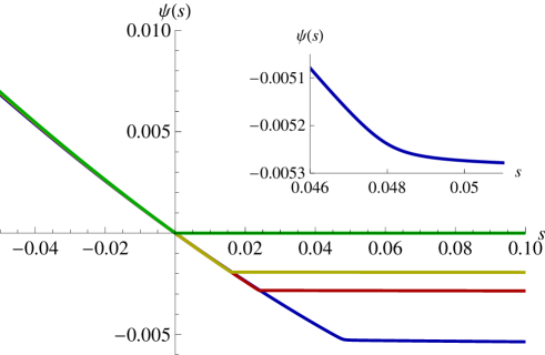
Figure 1: Dynamical free energy ψ(s)𝜓𝑠\psi(s) for c=0.3𝑐0.3c=0.3, L=50𝐿50L=50 (blue), L=100𝐿100L=100 (red), L=150𝐿150L=150 (yellow) and L=𝐿L=\infty (green). By locating numerically the maximum of ψ′′(s)superscript𝜓′′𝑠\psi^{\prime\prime}(s), we estimate that scsubscript𝑠cs_{\rm c} is equal to 0.04790.04790.0479... for L=50𝐿50L=50, 0.023900.023900.02390... for L=100𝐿100L=100 and 0.015910.015910.01591... for L=150𝐿150L=150. The value is close to 1/(2Lc(1c))12𝐿𝑐1𝑐1/(2Lc(1-c)), which takes 0.047620.047620.04762..., 0.023810.023810.02381... and 0.015870.015870.01587... for L=50,100𝐿50100L=50,100, and 150150150, respectively. The L=𝐿L=\infty curve is obtained from the variational formula (58). The inset illustrates the rounding of the cusp due to finite-size, for L=50𝐿50L=50, in the region of the transition.

We present in Fig. 1 the numerical evaluation of the dynamical free energy ψ(s)𝜓𝑠\psi(s) for c=0.3,L=50,100,150formulae-sequence𝑐0.3𝐿50100150c=0.3,L=50,100,150, obtained by solving the largest eigenvalue problem (8) numerically. We observe a remarkable point in each plot where ψ(s)𝜓𝑠\psi(s) presents a cusp, meaning that ψ′′(s)superscript𝜓′′𝑠\psi^{\prime\prime}(s) is sharply peaked. We note that the cusp is rounded in the finite-size systems as shown in the inset of Fig. 1, which becomes sharper as the system size becomes larger. We denote the corresponding s𝑠s by scsubscript𝑠cs_{\rm c}, and call it finite-size critical point:

scArgmaxψ′′(s).subscript𝑠cArgmaxsuperscript𝜓′′𝑠{s_{\rm c}\equiv{\rm Argmax}~{}\psi^{\prime\prime}(s).} (17)

As reported in Refs. [8, 9], scsubscript𝑠cs_{\rm c} deviates from the origin, but goes to zero as L𝐿L\to\infty.

We derive below an upper bound for a scaled critical point

λc=limLLsc.subscript𝜆𝑐subscript𝐿𝐿subscript𝑠c{\lambda_{c}=\lim_{L\to\infty}Ls_{\rm c}.} (18)

By taking s𝑠s\rightarrow\infty in (8), we obtain the asymptotic behavior of ψ(s)𝜓𝑠\psi(s) at large s𝑠s

limsψ(s)=1Lminn>0r(n)=c(L1)/L2.subscript𝑠𝜓𝑠1𝐿subscript𝑛0𝑟𝑛𝑐𝐿1superscript𝐿2\lim_{s\rightarrow\infty}\psi(s)=-\frac{1}{L}\min_{n>0}r(n)=-c(L-1)/L^{2}. (19)

Remarking now from (11) that ψ(s)𝜓𝑠\psi(s) is strictly decreasing, we obtain the inequality

ψ(s)>c(L1)/L2.𝜓𝑠𝑐𝐿1superscript𝐿2\psi(s)>-c(L-1)/L^{2}. (20)

On the other hand, by expanding ψ(s)𝜓𝑠\psi(s) around s=0𝑠0s=0, we obtain that

ψ(s)=reqsL+O(s2)=2(1c)c2s+O(s2).𝜓𝑠subscriptdelimited-⟨⟩𝑟eq𝑠𝐿𝑂superscript𝑠221𝑐superscript𝑐2𝑠𝑂superscript𝑠2\psi(s)=-\left\langle r\right\rangle_{\rm eq}\frac{s}{L}+O(s^{2})=-2(1-c)c^{2}s+O(s^{2}). (21)

Note that this expansion is valid only in the region around λ=0𝜆0\lambda=0 where ψ(s)𝜓𝑠\psi(s) remains analytic in the large size limit. To identify this region and define properly its scaling, let us now introduce the rescaled dynamical free energy [13, 14]

φL(λ)=Lψ(λ/L)subscript𝜑𝐿𝜆𝐿𝜓𝜆𝐿\varphi_{L}(\lambda)=L\psi(\lambda/L) (22)

The transition point scsubscript𝑠cs_{\rm c} now defines a critical value λc=limLLscsubscript𝜆csubscript𝐿𝐿subscript𝑠𝑐\lambda_{\rm c}=\lim_{L\to\infty}Ls_{c} where φ(λ)=limLφL(λ)subscript𝜑𝜆subscript𝐿subscript𝜑𝐿𝜆\varphi_{\infty}(\lambda)=\lim_{L\to\infty}\varphi_{L}(\lambda) presents a non-analyticity. The previous expansion (21) becomes

φL(λ)=2(1c)c2λ+O(λ2/L).subscript𝜑𝐿𝜆21𝑐superscript𝑐2𝜆𝑂superscript𝜆2𝐿\varphi_{L}(\lambda)=-2(1-c)c^{2}\lambda+O(\lambda^{2}/L). (23)

Thus one has φ(λ)=2(1c)c2λsubscript𝜑𝜆21𝑐superscript𝑐2𝜆\varphi_{\infty}(\lambda)=-2(1-c)c^{2}\lambda in the region around λ=0𝜆0\lambda=0 where φ(λ)subscript𝜑𝜆\varphi_{\infty}(\lambda) is analytic, while the inequality (20) yields φ(λ)csubscript𝜑𝜆𝑐\varphi_{\infty}(\lambda)\geq-c for all values of λ𝜆\lambda. This implies that φ(λ)subscript𝜑𝜆\varphi_{\infty}(\lambda) becomes non-analytic at a point λcsubscript𝜆c\lambda_{\rm c} bounded as

λc12c(1c)subscript𝜆c12𝑐1𝑐\lambda_{\rm c}\leq\frac{1}{2c(1-c)} (24)

Interestingly, this expression also gives a good approximation for scsubscript𝑠cs_{\rm c}: The behavior sc1/(2Lc(1c))similar-to-or-equalssubscript𝑠c12𝐿𝑐1𝑐s_{\rm c}\simeq 1/(2Lc(1-c)) can be checked numerically as displayed in Fig. 1. In Appendix A, building on our results, we shall derive the equality sc=1/(2Lc(1c))+O(1/L2)subscript𝑠c12𝐿𝑐1𝑐𝑂1superscript𝐿2s_{\rm c}=1/(2Lc(1-c))+O(1/L^{2}).

Remark last that in finite-dimensional FA models, such an approach also yields an upper bound for λcsubscript𝜆c\lambda_{\rm c} which however is not the value of λcsubscript𝜆c\lambda_{\rm c}, due to the complex interfacial spatial structure of the steady state around λcsubscript𝜆c\lambda_{\rm c} [13, 14].

2.3 The free energy difference at s=sc𝑠subscript𝑠cs=s_{\rm c} and the finite-size correction

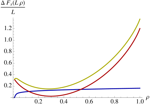
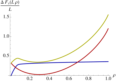
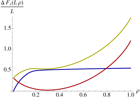
Let us now study numerical examples of the free energy difference for s=0.95sc𝑠0.95subscript𝑠c{s=0.95s_{\rm c}}, s=sc𝑠subscript𝑠cs=s_{\rm c} and s=1.05sc𝑠1.05subscript𝑠cs=1.05\,s_{\rm c}: in each subfigure of Fig. 2 are displayed the free energy difference ΔFs(ρL)/LΔsubscript𝐹𝑠𝜌𝐿𝐿\Delta F_{s}(\rho L)/L, the original free energy logPeq(ρL)/Lsubscript𝑃eq𝜌𝐿𝐿-\log P_{\rm eq}(\rho L)/L, and the modified one logPs(ρL)/Lsuperscript𝑃𝑠𝜌𝐿𝐿-\log P^{s}(\rho L)/L as functions of the density ρ𝜌\rho.

Refer to caption
Refer to caption
Refer to caption
Figure 2: The free energy difference ΔFs(ρL)/LΔsubscript𝐹𝑠𝜌𝐿𝐿\Delta F_{s}(\rho L)/L (blue), the original free energy logPeq(ρL)/Lsubscript𝑃eq𝜌𝐿𝐿-\log P_{\rm eq}(\rho L)/L (red) and the modified one logPs(ρL)/L=logPeq(ρL)/L+ΔFs(ρL)/Lsuperscript𝑃𝑠𝜌𝐿𝐿subscript𝑃eq𝜌𝐿𝐿Δsubscript𝐹𝑠𝜌𝐿𝐿-\log P^{s}(\rho L)/L=-\log P_{\rm eq}(\rho L)/L+\Delta F_{s}(\rho L)/L (yellow) for c=0.3,L=100formulae-sequence𝑐0.3𝐿100c=0.3,L=100. We set s=0.95sc𝑠0.95subscript𝑠cs=0.95s_{\rm c} (top), s=sc𝑠subscript𝑠cs=s_{\rm c} (middle) and s=1.05sc𝑠1.05subscript𝑠cs=1.05s_{\rm c} (bottom). In the L𝐿L\to\infty limit, those functions converge to analytical forms described by (33), (34) and (36), depicted in Fig. 4.

For s=sc𝑠subscript𝑠cs=s_{\rm c}, one observes that the modified free energy reaches its minimum value at the two values of the density ρ=n/L𝜌𝑛𝐿{\rho=n/L} of occupied sites characterizing the inactive (ρ0similar-to-or-equals𝜌0\rho\simeq 0) and the active (ρcsimilar-to-or-equals𝜌𝑐\rho\simeq c) configurations. This indicates that the first order phase transition observed along direction s𝑠s at s=sc𝑠subscript𝑠cs=s_{\rm c} also reflects itself in a first order coexistence in the density ρ𝜌\rho: precisely at s=sc𝑠subscript𝑠cs=s_{\rm c}, the two competing phases have the same weight. In this subsection, we consider the analytical expression of the free energy (difference). First, we derive the analytical expression of the free energy fs(ρ)limL1LlogPeqs(ρL)/Lsubscript𝑓𝑠𝜌subscript𝐿1𝐿subscriptsuperscript𝑃𝑠eq𝜌𝐿𝐿f_{s}(\rho)\equiv-\lim_{L\rightarrow\infty}\frac{1}{L}\log P^{s}_{\rm eq}(\rho L)/L at s=sc𝑠subscript𝑠𝑐s=s_{c}, which describes the distribution of particle occupation at the transition point in the infinite-size limit. Then, we derive the finite-size correction of these expressions, which will be used for deriving the scaling behavior of this first order phase transition in the next section.

We start with the eigenvalue equation (8). Since we focus on s=sc𝑠subscript𝑠𝑐s=s_{c}, we can set

Lψ(sc)=c+O(1/L),𝐿𝜓subscript𝑠c𝑐𝑂1𝐿L\psi(s_{\rm c})=-c+O(1/L), (25)

which leads to

ΦL(n+1)cnL(Ln)esc+ΦL(n1)(1c)Ln(n1)escsubscriptΦL𝑛1𝑐𝑛𝐿𝐿𝑛superscriptesubscript𝑠csubscriptΦL𝑛11𝑐𝐿𝑛𝑛1superscriptesubscript𝑠c\displaystyle\Phi_{\rm L}(n+1)\frac{cn}{L}(L-n){\rm e}^{-s_{\rm c}}+\Phi_{\rm L}(n-1)\frac{(1-c)}{L}n(n-1){\rm e}^{-s_{\rm c}}
ΦL(n)[cnL(Ln)+(1c)nL(n1)c+O(1/L)]=0.subscriptΦL𝑛delimited-[]𝑐𝑛𝐿𝐿𝑛1𝑐𝑛𝐿𝑛1𝑐𝑂1𝐿0\displaystyle-\Phi_{\rm L}(n)\left[c\frac{n}{L}(L-n)+(1-c)\frac{n}{L}(n-1)-c+O(1/L)\right]=0. (26)

Now, we assume the large deviation principle of ΦL(n)subscriptΦL𝑛\Phi_{\rm L}(n),

ΦL(n)=eLΔfsc(n/L)/2,subscriptΦL𝑛superscripte𝐿Δsubscript𝑓subscriptsc𝑛𝐿2{\Phi_{\rm L}(n)={\rm e}^{-L\Delta f_{\rm s_{\rm c}}(n/L)/2},} (27)

which defines ΔfscΔsubscript𝑓subscriptsc\Delta f_{\rm s_{\rm c}}. By substituting ΦL(n)subscriptΦL𝑛\Phi_{\rm L}(n) in (26) by the large deviation expression and evaluating the leading order with an assumption of differentiability of Δfsc(ρ)Δsubscript𝑓subscriptsc𝜌\Delta f_{\rm s_{\rm c}}(\rho), we obtain an equation for determining Δfsc(ρ)Δsubscript𝑓subscriptsc𝜌\Delta f_{\rm s_{\rm c}}(\rho). That is,

e(1/2)Δfsc(ρ)/ρcρ(1ρ)+e(1/2)Δfsc(ρ)/ρ(1c)ρ2superscripte12Δsubscript𝑓subscriptsc𝜌𝜌𝑐𝜌1𝜌superscripte12Δsubscript𝑓subscriptsc𝜌𝜌1𝑐superscript𝜌2\displaystyle{\rm e}^{-(1/2)\partial\Delta f_{\rm s_{\rm c}}(\rho)/\partial\rho}c\rho(1-\rho)+{\rm e}^{(1/2)\partial\Delta f_{\rm s_{\rm c}}(\rho)/\partial\rho}(1-c)\rho^{2}
[cρ(1ρ)+(1c)ρ2]=0.delimited-[]𝑐𝜌1𝜌1𝑐superscript𝜌20\displaystyle-\left[c\rho(1-\rho)+(1-c)\rho^{2}\right]=0. (28)

By solving this equation, we obtain two expressions of Δfsc(ρ)/ρΔsubscript𝑓subscriptsc𝜌𝜌\partial\Delta f_{\rm s_{\rm c}}(\rho)/\partial\rho as

Δfsc(ρ)/ρ=0Δsubscript𝑓subscriptsc𝜌𝜌0\partial\Delta f_{\rm s_{\rm c}}(\rho)/\partial\rho=0 (29)

and

Δfsc(ρ)/ρ=2log[(1c)ρc(1ρ)]=2fe(ρ)ρ,Δsubscript𝑓subscriptsc𝜌𝜌21𝑐𝜌𝑐1𝜌2subscript𝑓e𝜌𝜌\partial\Delta f_{\rm s_{\rm c}}(\rho)/\partial\rho=-2\log\left[\frac{(1-c)\rho}{c(1-\rho)}\right]=-2\frac{\partial f_{\rm e}(\rho)}{\partial\rho}, (30)

which leads to

Δfsc(ρ)=const.Δsubscript𝑓subscriptsc𝜌const\Delta f_{\rm s_{\rm c}}(\rho)=\rm const. (31)

and

Δfsc(ρ)=2fe(ρ)+const.Δsubscript𝑓subscriptsc𝜌2subscript𝑓e𝜌const\Delta f_{\rm s_{\rm c}}(\rho)=-2f_{\rm e}(\rho)+\rm const. (32)

We connect these two functions. We call the connecting point ρcsuperscriptsubscript𝜌c\rho_{\rm c}^{\infty}. By referring the numerical result in Fig. 2, we conjecture that Δfsc(ρ)Δsubscript𝑓subscriptsc𝜌\Delta f_{\rm s_{\rm c}}(\rho) becomes

Δfsc(ρ)=2fe(ρ)+2fe(0).Δsubscript𝑓subscriptsc𝜌2subscript𝑓e𝜌2subscript𝑓e0\Delta f_{\rm s_{\rm c}}(\rho)=-2f_{\rm e}(\rho)+2f_{\rm e}(0). (33)

for ρρc𝜌superscriptsubscript𝜌𝑐\rho\leq\rho_{c}^{\infty} and

Δfsc(ρ)=2fe(ρc)+2fe(0).Δsubscript𝑓subscriptsc𝜌2subscript𝑓esuperscriptsubscript𝜌c2subscript𝑓e0\Delta f_{\rm s_{\rm c}}(\rho)=-2f_{\rm e}(\rho_{\rm c}^{\infty})+2f_{\rm e}(0). (34)

for ρ>ρc𝜌superscriptsubscript𝜌c\rho>\rho_{\rm c}^{\infty}. Here, ρcsuperscriptsubscript𝜌c\rho_{\rm c}^{\infty} is determined from the condition of first order phase transition expressing here that the inactive (ρ0similar-to-or-equals𝜌0\rho\simeq 0) and the active (ρcsimilar-to-or-equals𝜌𝑐\rho\simeq c) configurations have the same weight

fe(c)+Δfsc(c)=fe(0)+Δfsc(0),subscript𝑓e𝑐Δsubscript𝑓subscriptsc𝑐subscript𝑓e0Δsubscript𝑓subscriptsc0f_{\rm e}(c)+\Delta f_{\rm s_{\rm c}}(c)=f_{\rm e}(0)+\Delta f_{\rm s_{\rm c}}(0), (35)

which leads to

2[(1ρc)log1ρc1c+ρclogρcc]=log(1c).2delimited-[]1superscriptsubscript𝜌c1superscriptsubscript𝜌c1𝑐superscriptsubscript𝜌csuperscriptsubscript𝜌𝑐𝑐1𝑐2\left[(1-\rho_{\rm c}^{\infty})\log\frac{1-\rho_{\rm c}^{\infty}}{1-c}+\rho_{\rm c}^{\infty}\log\frac{\rho_{c}^{\infty}}{c}\right]=-\log(1-c). (36)

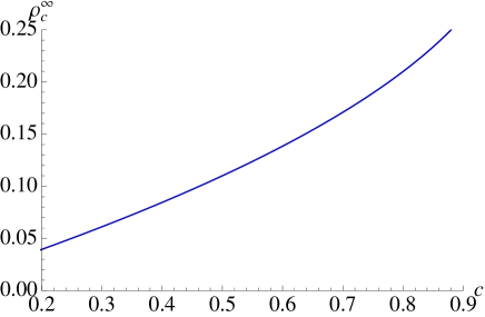
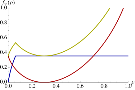
In Fig. 3, we plot ρcsuperscriptsubscript𝜌c\rho_{\rm c}^{\infty} as a function of c𝑐c. Also, in Fig. 4, we plot the obtained Δfsc(ρ)Δsubscript𝑓subscriptsc𝜌\Delta f_{\rm s_{\rm c}}(\rho) with fe(ρ)+Δfsc(ρ)subscript𝑓e𝜌Δsubscript𝑓subscriptsc𝜌f_{\rm e}(\rho)+\Delta f_{\rm s_{\rm c}}(\rho) and fe(ρ)subscript𝑓e𝜌f_{\rm e}(\rho) for c=0.3𝑐0.3c=0.3. From the figure, we understand that ρcsuperscriptsubscript𝜌c\rho_{\rm c}^{\infty} is a point of non-analyticity for the free energies: the distribution of the density ρ𝜌\rho of occupied sites in the system is naturally divided into two domains, namely, an active (ρ>ρc𝜌superscriptsubscript𝜌c\rho>\rho_{\rm c}^{\infty}) and an inactive (ρ<ρc𝜌superscriptsubscript𝜌c\rho<\rho_{\rm c}^{\infty}) domain.

Refer to caption
Figure 3: Connecting point ρcsuperscriptsubscript𝜌c\rho_{\rm c}^{\infty} in the infinite-size limit, as a function of c𝑐c, obtained from solving (36).
Refer to caption
Figure 4: The free energy fe(ρ)+Δfsc(ρ)subscript𝑓e𝜌Δsubscript𝑓subscriptsc𝜌f_{\rm e}(\rho)+\Delta f_{\rm s_{\rm c}}(\rho) (yellow) for s=sc𝑠subscript𝑠𝑐s=s_{c} and the modifying free energy Δfsc(ρ)Δsubscript𝑓subscriptsc𝜌\Delta f_{\rm s_{\rm c}}(\rho) (blue) for s=sc𝑠subscript𝑠𝑐s=s_{c} and the unbiased free energy fe(ρ)subscript𝑓e𝜌f_{\rm e}(\rho) (red). The point ρ=ρc𝜌superscriptsubscript𝜌c\rho=\rho_{\rm c}^{\infty} of non-analyticity of the two first functions is provided by the solution of equation (36).

Now, we consider the finite-size correction of the free energy. Those will be crucial to understand the finite-size scaling of the large deviation function, as explained in subsection 2.6. For this, we conjecture that the kink-like behavior of Δfsc(ρ)Δsubscript𝑓subscriptsc𝜌\Delta f_{\rm s_{\rm c}}(\rho) appears faster than O(1/L)𝑂1𝐿O(1/L) as suggested by the numerics presented in Fig. 7. From this, even for finite-size systems, we can define the active and the inactive regions. We denote the finite-size connecting point by ρcLsuperscriptsubscript𝜌𝑐𝐿\rho_{c}^{L}. Precisely, ρcLsuperscriptsubscript𝜌c𝐿\rho_{\rm c}^{L} is defined as

nncLPs(n)=n>ncLPs(n),subscript𝑛superscriptsubscript𝑛c𝐿superscript𝑃𝑠𝑛subscript𝑛superscriptsubscript𝑛c𝐿superscript𝑃𝑠𝑛\sum_{n\leq n_{\rm c}^{L}}P^{s}(n)=\sum_{n>n_{\rm c}^{L}}P^{s}(n), (37)

with the definition of nc=LρcLsubscript𝑛c𝐿superscriptsubscript𝜌c𝐿n_{\rm c}=\lfloor L\rho_{\rm c}^{L}\rfloor. Here, as shown in what follows, the distribution function Ps(n)superscript𝑃𝑠𝑛P^{s}(n) itself has a ρcLsuperscriptsubscript𝜌𝑐𝐿\rho_{c}^{L} dependence, so that the equation (37) can give a non-integer value for ρcLsuperscriptsubscript𝜌𝑐𝐿\rho_{c}^{L}. In order to obtain the next order correction of Δfsc(ρ)Δsubscript𝑓subscriptsc𝜌\Delta f_{\rm s_{\rm c}}(\rho) for each active and inactive region, we use a perturbation analysis. That is, for each region, we assume the following scaling

ΦL(n)=exp{(L/2)[Δfsc(n/L)+(1/L)Δfsc(1)(n/L)]}.subscriptΦL𝑛𝐿2delimited-[]Δsubscript𝑓subscript𝑠c𝑛𝐿1𝐿Δsuperscriptsubscript𝑓subscript𝑠c1𝑛𝐿\Phi_{\rm L}(n)=\exp\left\{-(L/2)\left[\Delta f_{s_{\rm c}}(n/L)+(1/L)\Delta f_{s_{\rm c}}^{(1)}(n/L)\right]\right\}. (38)

Expanding in powers of L𝐿L for large L𝐿L, we obtain the correction Δfsc(1)(n/L)Δsuperscriptsubscript𝑓subscript𝑠c1𝑛𝐿\Delta f_{s_{\rm c}}^{(1)}(n/L) as

Δfsc(1)(ρ)=logρ(1ρ)(cr)2ρ(12c)c(1c)+const.Δsuperscriptsubscript𝑓subscript𝑠c1𝜌𝜌1𝜌superscript𝑐𝑟2𝜌12𝑐𝑐1𝑐const\Delta f_{s_{\rm c}}^{(1)}(\rho)=-\log\frac{\rho(1-\rho)}{(c-r)^{2}}-\frac{\rho(1-2c)}{c(1-c)}+\rm const. (39)

for ρρcL𝜌superscriptsubscript𝜌c𝐿\rho\leq\rho_{\rm c}^{L}, and

Δfsc(1)(ρ)=2[ρ(2c1)2c(1c)logρ]+const.Δsuperscriptsubscript𝑓subscript𝑠c1𝜌2delimited-[]𝜌2𝑐12𝑐1𝑐𝜌const\Delta f_{s_{\rm c}}^{(1)}(\rho)=-2\left[\frac{\rho(2c-1)}{2c(1-c)}-\log\rho\right]+\rm const. (40)

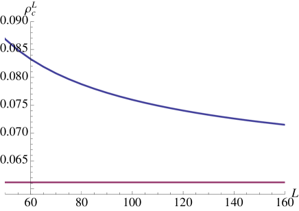
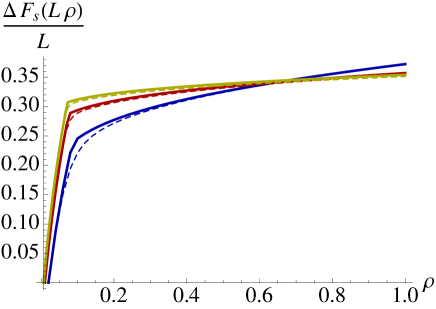
for ρ>ρcL𝜌superscriptsubscript𝜌𝑐𝐿\rho>\rho_{c}^{L}. See Appendix B for the derivation of these expressions. The two constants in (39) and (40) are determined from the conditions Δfsc(1)(1/L)=0Δsuperscriptsubscript𝑓subscript𝑠c11𝐿0\Delta f_{s_{\rm c}}^{(1)}(1/L)=0, and limρρcLΔfsc(1)(ρ)=limρρcLΔfsc(1)(ρ)subscript𝜌superscriptsubscript𝜌c𝐿Δsuperscriptsubscript𝑓subscript𝑠c1𝜌subscript𝜌superscriptsubscript𝜌c𝐿Δsuperscriptsubscript𝑓subscript𝑠c1𝜌\lim_{\rho\rightarrow\rho_{\rm c}^{L}}\Delta f_{s_{\rm c}}^{(1)}(\rho)=\lim_{\rho\rightarrow\rho_{\rm c}^{L}}\Delta f_{s_{\rm c}}^{(1)}(\rho). We note that the latter constant depends on ρcLsuperscriptsubscript𝜌c𝐿\rho_{\rm c}^{L}. In Fig. 5, we plot numerical examples of ρcLsuperscriptsubscript𝜌c𝐿\rho_{\rm c}^{L} obtained from (37-40) as a function of L𝐿L, together with the limiting value ρcsuperscriptsubscript𝜌c\rho_{\rm c}^{\infty}, which is the solution of (36). In Fig. 6, we compare our finite-size free energy with the numerical results obtained by direct diagonalization, for c=0.3𝑐0.3c=0.3, s=sc𝑠subscript𝑠cs=s_{\rm c}, L=50,100,150𝐿50100150L=50,100,150. The agreement of both results improves as L𝐿L increases.

Refer to caption
Figure 5: Numerical example illustrating the importance of finite-size corrections for ρcLsuperscriptsubscript𝜌c𝐿\rho_{\rm c}^{L} (in blue), compared to its infinite-size limit ρcsuperscriptsubscript𝜌c\rho_{\rm c}^{\infty} (in purple) for c=0.3𝑐0.3c=0.3.
Refer to caption
Figure 6: The finite-size correction of the free energy difference for c=0.3𝑐0.3c=0.3, s=sc𝑠subscript𝑠cs=s_{\rm c}, L=50𝐿50L=50 (in blue), L=100𝐿100L=100 (red) and L=150𝐿150L=150 (yellow). We plot analytical finite-size free energy difference obtained from (39) and (40) as solid lines. We also plot the exact numerical results as dashed lines. One observes the emergence of the non-analytic point at ρcLsuperscriptsubscript𝜌c𝐿\rho_{\rm c}^{L} as L𝐿L becomes large.

2.4 Scaling function around s=sc𝑠subscript𝑠cs=s_{\rm c}

As seen in the previous section, the system also displays a phase coexistence in the density ρ=n/L𝜌𝑛𝐿\rho=n/L of occupied sites, which plays a role similar to the mean magnetization in the Ising model. For the equilibrium ferromagnet model, the scaling functions describing finite-size scaling around the first order phase transition point have been determined [16, 17]. However, even though our system presents a first order phase transition, it is not trivial to determine such scaling functions because of the asymmetry of the scalings in the active and inactive phases. In what follows, we study the finite-size scaling behavior in our system.

To do so, we start by considering the statistical properties of the mean occupation n/L𝑛𝐿n/L. We denote by ρ(s)𝜌𝑠\rho(s) its expectation value

ρ(s)=n(n/L)Ps(n),𝜌𝑠subscript𝑛𝑛𝐿superscript𝑃𝑠𝑛\rho(s)=\sum_{n}(n/L)P^{s}(n), (41)

and by χ(s)𝜒𝑠\chi(s) its variance

χ(s)=Ln(n/Lρ(s))2Ps(n).𝜒𝑠𝐿subscript𝑛superscript𝑛𝐿𝜌𝑠2superscript𝑃𝑠𝑛\chi(s)=L\sum_{n}(n/L-\rho(s))^{2}P^{s}(n). (42)

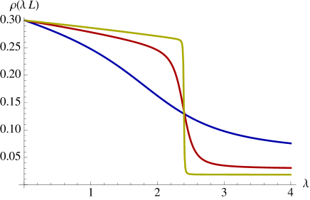
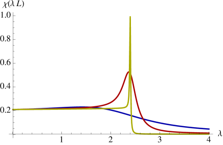
Examples of these functions are shown in Fig. 7, and the latter illustrate how the first order transition materializes around s=sc𝑠subscript𝑠cs=s_{\rm c}.

Refer to caption
Refer to caption
Figure 7: The expectation value ρ(λL)𝜌𝜆𝐿\rho(\lambda L) (41) (top) and the variance (42) χ(λL)𝜒𝜆𝐿\chi(\lambda L) (bottom) of the mean occupation n/L𝑛𝐿n/L in the s𝑠s-modified equilibrium state, plotted as a function of the rescaled variable λ=s/L𝜆𝑠𝐿\lambda=s/L. We set c=0.3𝑐0.3c=0.3 and L=20𝐿20L=20 (blue), L=40𝐿40L=40 (red) and L=60𝐿60L=60 (yellow). The position of the peak of χ(s)𝜒𝑠\chi(s) defines the value of scsubscript𝑠cs_{\rm c}, which appears on the graphs as a function of λ𝜆\lambda at a value close to the critical λc=1/(2c(1c))subscript𝜆c12𝑐1𝑐\lambda_{\rm c}=1/(2c(1-c)) derived in Section 2.2. For example, the peak occurs approximately at λ=2.398𝜆2.398\lambda=2.398... for L=60𝐿60L=60, which is close to the corresponding λc2.381similar-to-or-equalssubscript𝜆c2.381\lambda_{\rm c}\simeq 2.381...

One observes in particular that the width of the first order coexistence region shrinks as the system size L𝐿L becomes large. To estimate this dependence in L𝐿L, we define a scaling ratio κ𝜅\kappa as

κ=ρ(s)/s|s=sc,𝜅evaluated-at𝜌𝑠𝑠𝑠subscript𝑠c\kappa=-\partial\rho(s)/\partial s|_{s=s_{\rm c}}, (43)

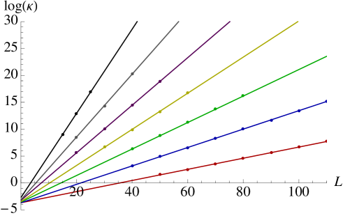
which is inversely proportional to the width of the first order coexistence region, and diverges as L𝐿L\to\infty. The logarithm of κ𝜅\kappa for various values c𝑐c is represented as a function of L𝐿L in Fig. 8.

Refer to caption
Figure 8: The logarithm of the scaling ratio κ𝜅\kappa defined in (43) as a function of L𝐿L for c=0.2𝑐0.2c=0.2 (red), c=0.3𝑐0.3c=0.3 (blue), c=0.4𝑐0.4c=0.4 (green), c=0.5𝑐0.5c=0.5 (yellow), c=0.6𝑐0.6c=0.6 (purple), c=0.7𝑐0.7c=0.7 (gray) and c=0.8𝑐0.8c=0.8 (black). Dots were obtained by solving the eigenvalue equation (8) numerically. Solid lines are linear fits.

We find that these logarithms are increasing linear functions of L𝐿L. It indicates that the width of the first order coexistence region (illustrated in Fig. 7) shrinks exponentially with the system size L𝐿L.

Next, we seek for the scaling functions of ρ(s)𝜌𝑠\rho(s) and χ(s)𝜒𝑠\chi(s) in the coexistence region. For this purpose, we introduce a scaling variable x𝑥x as

x=κ(ssc).𝑥𝜅𝑠subscript𝑠cx=\kappa(s-s_{\rm c}). (44)

Correspondingly, the rescaled expectation value and variance are defined as

ρ~(x)=ρ(xκ1+sc)~𝜌𝑥𝜌𝑥superscript𝜅1subscript𝑠c\tilde{\rho}(x)=\rho(x\kappa^{-1}+s_{\rm c}) (45)

and

χ~(x)=χ(xκ1+sc)/χ(sc),~𝜒𝑥𝜒𝑥superscript𝜅1subscript𝑠c𝜒subscript𝑠c\tilde{\chi}(x)=\chi(x\kappa^{-1}+s_{\rm c})/\chi(s_{\rm c}), (46)

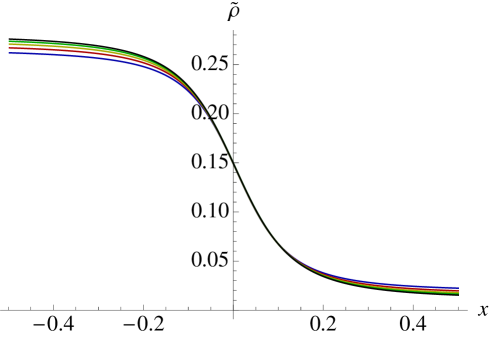
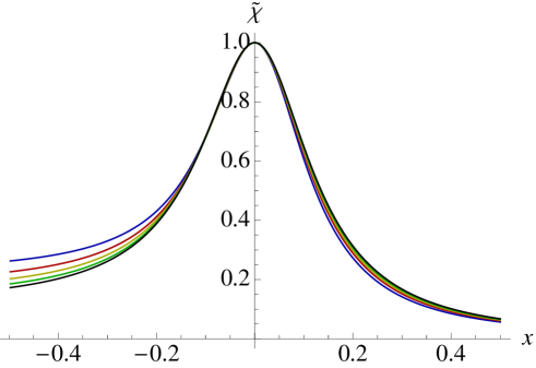
respectively. These functions are plotted for large values of L𝐿L in Fig. 9, thus illustrating their expected collapse as L𝐿L becomes large.

Refer to caption
Refer to caption
Figure 9: The scaling functions ρ~(x)=ρ(xκ1+sc)~𝜌𝑥𝜌𝑥superscript𝜅1subscript𝑠c\tilde{\rho}(x)=\rho(x\kappa^{-1}+s_{\rm c}) (top) and χ~(x)=χ(xκ1+sc)/χ(sc)~𝜒𝑥𝜒𝑥superscript𝜅1subscript𝑠c𝜒subscript𝑠c\tilde{\chi}(x)=\chi(x\kappa^{-1}+s_{\rm c})/\chi(s_{\rm c}) (bottom) for c=0.3𝑐0.3c=0.3 and for various L𝐿L. The blue, red, green, yellow, and black lines correspond to L=60,70,80,90𝐿60708090L=60,70,80,90, and L=100𝐿100L=100, respectively.

2.5 A variational formula in the infinite system-size limit

In the previous section, we found numerically that the scaling functions are well-defined with an exponential rescaling with the system size. Hereafter, we discuss how to derive those scaling properties analytically. With this purpose in mind, we consider the variational principle (10). We introduce a variational function Φ~L(n)subscript~ΦL𝑛\tilde{\Phi}_{\rm L}(n) as

Φ~L(n)=Φ0(n)Peq(n)1/2.subscript~ΦL𝑛superscriptΦ0𝑛subscript𝑃eqsuperscript𝑛12\tilde{\Phi}_{\rm L}(n)=\Phi^{0}(n)P_{\rm eq}(n)^{-1/2}. (47)

By changing the variational parameter Φ0superscriptΦ0\Phi^{0} to Φ~Lsubscript~ΦL\tilde{\Phi}_{\rm L}, we rewrite (10) as

Lψ(s)=maxΦ~L>0nP~(n)nΦ~L(n)Wn,nΦ~L(n)1,𝐿𝜓𝑠subscriptsubscript~ΦL0subscriptsuperscript𝑛~𝑃superscript𝑛subscript𝑛subscript~ΦL𝑛subscript𝑊𝑛superscript𝑛subscript~ΦLsuperscriptsuperscript𝑛1L\psi(s)=\max_{\tilde{\Phi}_{\rm L}>0}\sum_{n^{\prime}}\widetilde{P}(n^{\prime})\sum_{n}\tilde{\Phi}_{\rm L}(n)W_{n,n^{\prime}}\tilde{\Phi}_{\rm L}(n^{\prime})^{-1}, (48)

where the distribution function P~(n)~𝑃𝑛\widetilde{P}(n) is defined as

P~(n)=Peq(n)Φ~L(n)2n~Peq(n~)Φ~L(n~)2.~𝑃𝑛subscript𝑃eq𝑛subscript~ΦLsuperscript𝑛2subscript~𝑛subscript𝑃eq~𝑛subscript~ΦLsuperscript~𝑛2\widetilde{P}(n)=\frac{P_{\rm eq}(n)\tilde{\Phi}_{\rm L}(n)^{2}}{\sum_{\tilde{n}}P_{\rm eq}(\tilde{n})\tilde{\Phi}_{\rm L}(\tilde{n})^{2}}. (49)

We note that since, in (10), the optimal Φ~Lsubscript~ΦL\tilde{\Phi}_{\rm L} corresponds to the largest eigenvector ΦLsubscriptΦL\Phi_{\rm L}, the optimal distribution function P~~𝑃\widetilde{P} is equal to the modified equilibrium distribution function (15). Extensions of such variational principle are valid not only for equilibrium dynamics but also for nonequilibrium dynamics that violate the detailed balance condition. We refer the reader to Ref. [29] for details. In this section, before considering the finite-size scaling properties, we start by considering the L𝐿L\rightarrow\infty limit by assuming a large deviation principle in the optimal modified system holds.

Let us now introduce, similarly to (16), a variational function ΔF~Δ~𝐹\Delta\widetilde{F} as

ΔF~(n)=2logΦ~L(n),Δ~𝐹𝑛2subscript~ΦL𝑛\Delta\widetilde{F}(n)=-2\log\tilde{\Phi}_{\rm L}(n), (50)

and change the variational parameter Φ~Lsubscript~ΦL\tilde{\Phi}_{\rm L} to ΔF~Δ~𝐹\Delta\widetilde{F}. We note that the optimal ΔF~Δ~𝐹\Delta\widetilde{F} is equal to the free energy difference ΔFsΔsubscript𝐹𝑠\Delta F_{s} defined in (16). The extremalization principle (48) can be rewritten as

ψ(s)=1LmaxΔF~nP~(n)[r~(n)r(n)],𝜓𝑠1𝐿subscriptΔ~𝐹subscript𝑛~𝑃𝑛delimited-[]~𝑟𝑛𝑟𝑛\psi(s)=\frac{1}{L}\max_{\Delta\widetilde{F}}\sum_{n}\widetilde{P}(n)\left[\tilde{r}(n)-r(n)\right], (51)

where r~(n)~𝑟𝑛\tilde{r}(n) is defined as

r~(n)~𝑟𝑛\displaystyle\tilde{r}(n) =\displaystyle= nc(1nL)e12[ΔF~(n+1)ΔF~(n)]s𝑛𝑐1𝑛𝐿superscripte12delimited-[]Δ~𝐹𝑛1Δ~𝐹𝑛𝑠\displaystyle nc\left(1-\frac{n}{L}\right){\rm e}^{-\frac{1}{2}[\Delta\widetilde{F}(n+1)-\Delta\widetilde{F}(n)]-s} (52)
+n(1c)(nL1L)e12[ΔF~(n1)ΔF~(n)]s.𝑛1𝑐𝑛𝐿1𝐿superscripte12delimited-[]Δ~𝐹𝑛1Δ~𝐹𝑛𝑠\displaystyle\ +n(1-c)\left(\frac{n}{L}-\frac{1}{L}\right){\rm e}^{-\frac{1}{2}[\Delta\widetilde{F}(n-1)-\Delta\widetilde{F}(n)]-s}.

Now, we assume that the optimal modified distribution P~~𝑃\widetilde{P} scales, in the large L𝐿L asymptotics, by following the large deviation form

P~(n)eL[fe(n/L)+f~(n/L)],similar-to~𝑃𝑛superscripte𝐿delimited-[]subscript𝑓e𝑛𝐿~𝑓𝑛𝐿\widetilde{P}(n)\sim{\rm e}^{-L\left[f_{\rm e}(n/L)+\tilde{f}(n/L)\right]}, (53)

where f~(ρ)~𝑓𝜌\tilde{f}(\rho) is an unknown function we determine below. This indicates that the variational function ΔF~(n)Δ~𝐹𝑛\Delta\widetilde{F}(n) scales as Lf~(ρ)𝐿~𝑓𝜌L\tilde{f}(\rho) with ρ=n/L𝜌𝑛𝐿\rho=n/L, as L𝐿L\to\infty. From these assumptions, (52) is rewritten as

r~(Lρ)L=es[ρc(1ρ)e12f~(ρ)+ρ2(1c)e12f~(ρ)]+O(1/L)~𝑟𝐿𝜌𝐿superscripte𝑠delimited-[]𝜌𝑐1𝜌superscripte12superscript~𝑓𝜌superscript𝜌21𝑐superscripte12superscript~𝑓𝜌𝑂1𝐿\frac{\tilde{r}(L\rho)}{L}={\rm e}^{-s}\left[\rho c\left(1-\rho\right){\rm e}^{-\frac{1}{2}{\tilde{f}}^{\prime}\!(\rho)}+\rho^{2}(1-c){\rm e}^{\frac{1}{2}{\tilde{f}}^{\prime}\!(\rho)}\right]+O(1/L) (54)

where f~(ρ)=f~(ρ)ρsuperscript~𝑓𝜌~𝑓𝜌𝜌{\tilde{f}}^{\prime}\!(\rho)=\frac{\partial\tilde{f}(\rho)}{\partial\rho}. By substituting this into (51) and evaluating the summation within the saddle point approximation, we obtain, up to terms in O(1/L)𝑂1𝐿O(1/L)

ψ(s)𝜓𝑠\displaystyle\psi(s)
=maxf~>0𝑑ρ{es[ρc(1ρ)e12f~(ρ)+ρ2(1c)e12f~(ρ)]r(Lρ)/L}eL[fe(ρ)+f~(ρ)]𝑑ρeL[fe(ρ)+f~(ρ)]absentsubscript~𝑓0differential-d𝜌superscripte𝑠delimited-[]𝜌𝑐1𝜌superscripte12superscript~𝑓𝜌superscript𝜌21𝑐superscripte12superscript~𝑓𝜌𝑟𝐿𝜌𝐿superscripte𝐿delimited-[]subscript𝑓e𝜌~𝑓𝜌differential-d𝜌superscripte𝐿delimited-[]subscript𝑓e𝜌~𝑓𝜌\displaystyle=\max_{\tilde{f}>0}\frac{\displaystyle\int\!d\rho\,\Big{\{}{\rm e}^{-s}\Big{[}\rho c\big{(}1-\rho\big{)}{\rm e}^{-\frac{1}{2}{\tilde{f}}^{\prime}\!(\rho)}+\rho^{2}(1-c){\rm e}^{\frac{1}{2}{\tilde{f}}^{\prime}\!(\rho)}\Big{]}-r(L\rho)/L\Big{\}}{\rm e}^{-L[f_{\rm e}(\rho)+\tilde{f}(\rho)]}}{\displaystyle\int\!d\rho\,{\rm e}^{-L[f_{\rm e}(\rho)+\tilde{f}(\rho)]}} (55)

Here fe(ρ)subscript𝑓e𝜌f_{\rm e}(\rho) is the large deviation function (6). We now evaluate the integrals over ρ𝜌\rho through the saddle-point method. From (54), we read that the exponential dependence in L𝐿L of the numerator and the denominator of (55) is the same. Assuming that the optimal function fe(ρ)+f~(ρ)subscript𝑓e𝜌~𝑓𝜌f_{\rm e}(\rho)+\tilde{f}(\rho) reaches its minimum at a unique point ρ0superscript𝜌0\rho^{0}, we have that the numerator and the denominator of (55) are both dominated by ρ=ρ0𝜌superscript𝜌0\rho=\rho^{0}. With the condition

f~(ρ0)+fe(ρ0)=0,superscript~𝑓superscript𝜌0superscriptsubscript𝑓esuperscript𝜌00{\tilde{f}}^{\prime}\!(\rho^{0})+{f_{\rm e}}^{\prime}(\rho^{0})=0, (56)

this leads to the variational principle

ψ(s)=max0ρ01{es[ρ0c(1ρ0)e12f~(ρ0)+(ρ0)2(1c)e12f~(ρ0)]r(Lρ0)/L}𝜓𝑠subscript0superscript𝜌01superscripte𝑠delimited-[]superscript𝜌0𝑐1superscript𝜌0superscripte12superscript~𝑓superscript𝜌0superscriptsuperscript𝜌021𝑐superscripte12superscript~𝑓superscript𝜌0𝑟𝐿superscript𝜌0𝐿\psi(s)=\max_{0\leq\rho^{0}\leq 1}\Big{\{}{\rm e}^{-s}\Big{[}\rho^{0}c\big{(}1-\rho^{0}\big{)}{\rm e}^{-\frac{1}{2}{\tilde{f}}^{\prime}\!(\rho^{0})}+(\rho^{0})^{2}(1-c){\rm e}^{\frac{1}{2}{\tilde{f}}^{\prime}\!(\rho^{0})}\Big{]}-r(L\rho^{0})/L\Big{\}} (57)

Finally, by substituting (56) into (57) and using the definition (6) of fe(ρ)subscript𝑓e𝜌f_{\rm e}(\rho), we arrive at

ψ(s)=max0ρ1{2esρ3(1ρ)c(1c)[ρc(1ρ)+(1c)ρ2]}+O(1/L)𝜓𝑠subscript0𝜌12superscripte𝑠superscript𝜌31𝜌𝑐1𝑐delimited-[]𝜌𝑐1𝜌1𝑐superscript𝜌2𝑂1𝐿\psi(s)=\max_{0\leq\rho\leq 1}\left\{2{\rm e}^{-s}\sqrt{\rho^{3}(1-\rho)c(1-c)}-\left[\rho c(1-\rho)+(1-c)\rho^{2}\right]\right\}+O(1/L) (58)

Such variational formula describes the large-size behavior of large deviation of a wide class of stochastic models on the complete graph [24, 8, 9] or quantum annealing models [22]. In Fig. 1, the obtained limLψ(s)subscript𝐿𝜓𝑠\lim_{L\to\infty}\psi(s), whose transitions occurs at sc=0superscriptsubscript𝑠c0s_{\rm c}^{\infty}=0, is compared to finite-size results obtained by numerical diagonalization.

We now discuss how to extend the discussion presented in this subsection so as to obtain the finite-size scaling. A blunt perturbation in 1/L1𝐿1/L around (58) cannot be performed directly, since for instance it cannot describe how the O(L0)𝑂superscript𝐿0O(L^{0}) discontinuity of K(s)𝐾𝑠K(s) at sc=0superscriptsubscript𝑠𝑐0s_{c}^{\infty}=0 is rounded at large but finite L𝐿L. More generically, the free energy difference ΔFsΔsubscript𝐹𝑠\Delta F_{s} defined in (16), which allows one to recover ψ(s)𝜓𝑠\psi(s), is exactly 0 at s=0𝑠0s=0. One could thus expect that ΔFs/L=O(1/L)Δsubscript𝐹𝑠𝐿𝑂1𝐿\Delta F_{s}/L=O(1/L) at the transition point, using that sc=O(1/L)subscript𝑠c𝑂1𝐿s_{\rm c}=O(1/L) (Section 2.2). However, because of the non-analyticity of ΔFs/LΔsubscript𝐹𝑠𝐿\Delta F_{s}/L with respect to s𝑠s around the transition point scsubscript𝑠cs_{\rm c}, one has in fact ΔFs/L=O(1)Δsubscript𝐹𝑠𝐿𝑂1\Delta F_{s}/L=O(1), as discussed in Section 2.3. This explains the breakdown of a 1/L1𝐿1/L expansion of (58). In the next section, we propose a new method to overcome those difficulties without relying on a perturbative approach.

2.6 Analytical expressions for the scaling functions

Let us first consider the coexistence point s=sc𝑠subscript𝑠cs=s_{\rm c}. We use the finite-size correction of the free energy obtained in Section 2.3. We first define the finite-size free energy difference for each region as

fi(ρ)=Δfsc(ρ)+1LΔfsc(1)(ρ)subscript𝑓i𝜌Δsubscript𝑓subscript𝑠c𝜌1𝐿Δsuperscriptsubscript𝑓subscriptsc1𝜌f_{\rm i}(\rho)=\Delta f_{s_{{\rm c}}}(\rho)+\frac{1}{L}\Delta f_{\rm s_{c}}^{(1)}(\rho) (59)

for ρρcL𝜌superscriptsubscript𝜌c𝐿\rho\leq\rho_{\rm{\rm c}}^{L}

fa(ρ)=Δfsc(ρ)+1LΔfsc(1)(ρ)subscript𝑓a𝜌Δsubscript𝑓subscript𝑠c𝜌1𝐿Δsuperscriptsubscript𝑓subscriptsc1𝜌f_{\rm a}(\rho)=\Delta f_{s_{{\rm c}}}(\rho)+\frac{1}{L}\Delta f_{\rm s_{c}}^{(1)}(\rho) (60)

for ρ>ρcL𝜌superscriptsubscript𝜌c𝐿\rho>\rho_{\rm{\rm c}}^{L}. Then, the corresponding distribution function is

Psc(n)=Pi(n) 1nncL+Pa(n) 1n>ncL,superscript𝑃subscript𝑠c𝑛subscript𝑃i𝑛subscript1𝑛superscriptsubscript𝑛c𝐿subscript𝑃a𝑛subscript1𝑛superscriptsubscript𝑛c𝐿P^{s_{\rm c}}(n)=P_{\rm i}(n)\,\mathbf{1}_{n\leq n_{\rm c}^{L}}+P_{\rm a}(n)\,\mathbf{1}_{n>n_{\rm c}^{L}}, (61)

where Pi(n)subscript𝑃i𝑛P_{\rm i}(n) and Pa(n)subscript𝑃a𝑛P_{\rm a}(n) are defined as

Pi(n)=1Zi+ZaPeq(n)eLfi(n/L)subscript𝑃i𝑛1subscript𝑍isubscript𝑍asubscript𝑃eq𝑛superscripte𝐿subscript𝑓i𝑛𝐿P_{\rm i}(n)=\frac{1}{Z_{\rm i}+Z_{\rm a}}P_{\rm eq}(n){\rm e}^{-Lf_{\rm i}(n/L)} (62)
Pa(n)=1Zi+ZaPeq(n)eLfa(n/L)subscript𝑃a𝑛1subscript𝑍isubscript𝑍asubscript𝑃eq𝑛superscripte𝐿subscript𝑓a𝑛𝐿P_{\rm a}(n)=\frac{1}{Z_{\rm i}+Z_{\rm a}}P_{\rm eq}(n){\rm e}^{-Lf_{\rm a}(n/L)} (63)

with the normalization constant

Zi=nncPeq(n)eLfi(n/L),subscript𝑍isubscript𝑛subscript𝑛csubscript𝑃eq𝑛superscripte𝐿subscript𝑓i𝑛𝐿Z_{{\rm i}}=\sum_{n\leq n_{\rm c}}P_{\rm eq}(n){\rm e}^{-Lf_{\rm i}(n/L)}, (64)
Za=n>ncPeq(n)eLfa(n/L).subscript𝑍asubscript𝑛subscript𝑛csubscript𝑃eq𝑛superscripte𝐿subscript𝑓a𝑛𝐿Z_{{\rm a}}=\sum_{n>n_{\rm c}}P_{\rm eq}(n){\rm e}^{-Lf_{\rm a}(n/L)}. (65)

Here, we note Zi=Zasubscript𝑍isubscript𝑍aZ_{\rm i}=Z_{\rm a} from the definition (37) of ρcLsuperscriptsubscript𝜌c𝐿\rho_{\rm c}^{L}. In this system, there naturally arise two regions, nnc𝑛subscript𝑛cn\leq n_{\rm c} and n>nc𝑛subscript𝑛cn>n_{\rm c}, which represent inactive phase and active phase, respectively. As seen below, this separation plays an important role in the exponentially fast scaling of Section 2.4.

By using the result at s=sc𝑠subscript𝑠cs=s_{\rm c}, we consider the region around scsubscript𝑠cs_{\rm c} (sscsimilar-to𝑠subscript𝑠cs\sim s_{\rm c}). Here, we propose an Ansatz. That is, the distribution function around scsubscript𝑠cs_{\rm c} is written as

Ps(n)=[1+a(s)]δnncPi(n)+[1a(s)]δn>ncPa(n),superscript𝑃𝑠𝑛delimited-[]1superscript𝑎𝑠subscript𝛿𝑛subscript𝑛csubscript𝑃i𝑛delimited-[]1superscript𝑎𝑠subscript𝛿𝑛subscript𝑛csubscript𝑃a𝑛P^{s}(n)=[1+a^{*}(s)]\delta_{n\leq n_{\rm c}}P_{\rm i}(n)+[1-a^{*}(s)]\delta_{n>n_{\rm c}}P_{\rm a}(n), (66)

where a(s)superscript𝑎𝑠a^{*}(s) is a ‘mixing function’ to determine. This Ansatz is inspired by the mathematically-proved description of static and classical equilibrium first-order transitions in the coexistence region as described in [16, 17] based on a Gibbs distribution picture. We should mention that in contrast to [16, 17], our full distribution Ps(n)superscript𝑃𝑠𝑛P^{s}(n) does not describe a superposition between two elementary distributions, but a separation of the space of occupation number n𝑛n into two regions presenting distributions of different nature. Also, we stress that the main difference between our method and their method appears in the mixing function a(s)superscript𝑎𝑠a^{*}(s), which is be determined by a variational principle as shown below. The dynamical thermodynamic formalism has a variational principle which determines the stationary state, in contrast to the equilibrium thermodynamics. The mixing function a(s)superscript𝑎𝑠a^{*}(s) reflects this inevitable difference between these two thermodynamics.

To our knowledge, the Ansatz (66) has not been used up to now in the dynamical approach we follow. In physical terms, the Ansatz (66) allows to handle the difficulty at the core of the extension of the infinite-size method presented in Section 2.5. In the infinite-size limit, the variational maximum (48) is dominated by the most probable value of the occupation density ρ𝜌\rho, yielding (58). In finite-size this image however breaks down in the vicinity of s=sc𝑠subscript𝑠cs=s_{\rm c}, where the active and inactive densities ρ0similar-to-or-equals𝜌0\rho\simeq 0 and ρcsimilar-to-or-equals𝜌𝑐\rho\simeq c are in competition, and finer details than the mere maximum of the distribution of ρ𝜌\rho have to be taken into account at large but finite L𝐿L. The Ansatz (66) describes the continuous transition, as s𝑠s increases, from the active to the inactive distribution of density.

The distribution function (66) satisfies the normalization condition because Zi=Zasubscript𝑍isubscript𝑍aZ_{\rm i}=Z_{\rm a}. From this expression and the relation (15), we obtain ΦL(n)subscriptΦL𝑛\Phi_{\rm L}(n) (or the free energy difference ΔFs(n)Δsubscript𝐹𝑠𝑛\Delta F_{s}(n)) as

ΦL(n)δnnc1+a(s)eLfi(n/L)/2+δn>nc1a(s)eLfa(n/L)/2,proportional-tosubscriptΦL𝑛subscript𝛿𝑛subscript𝑛c1superscript𝑎𝑠superscripte𝐿subscript𝑓i𝑛𝐿2subscript𝛿𝑛subscript𝑛c1superscript𝑎𝑠superscripte𝐿subscript𝑓a𝑛𝐿2\Phi_{\rm L}(n)\propto\delta_{n\leq n_{\rm c}}\sqrt{1+a^{*}(s)}{\rm e}^{-Lf_{\rm i}(n/L)/2}+\delta_{n>n_{\rm c}}\sqrt{1-a^{*}(s)}{\rm e}^{-Lf_{\rm a}(n/L)/2}, (67)

and the expectation values ρ(s)𝜌𝑠\rho(s), χ(s)𝜒𝑠\chi(s) around scsubscript𝑠cs_{\rm c} as

ρ(s)=ρi2[1+a(s)]+ρa2[1a(s)],𝜌𝑠subscriptdelimited-⟨⟩𝜌i2delimited-[]1superscript𝑎𝑠subscriptdelimited-⟨⟩𝜌a2delimited-[]1superscript𝑎𝑠\rho(s)=\frac{\left\langle\rho\right\rangle_{\rm i}}{2}\left[1+a^{*}(s)\right]+\frac{\left\langle\rho\right\rangle_{\rm a}}{2}\left[1-a^{*}(s)\right], (68)
χ(s)=L{ρ2i2[1+a(s)]+ρ2a2[1a(s)]ρ(s)2},𝜒𝑠𝐿subscriptdelimited-⟨⟩superscript𝜌2i2delimited-[]1superscript𝑎𝑠subscriptdelimited-⟨⟩superscript𝜌2a2delimited-[]1superscript𝑎𝑠𝜌superscript𝑠2\chi(s)=L\left\{\frac{\left\langle\rho^{2}\right\rangle_{\rm i}}{2}\left[1+a^{*}(s)\right]+\frac{\left\langle\rho^{2}\right\rangle_{\rm a}}{2}\left[1-a^{*}(s)\right]-\rho(s)^{2}\right\}, (69)

where isubscripti\left\langle\ \right\rangle_{\rm i} and asubscripta\left\langle\ \right\rangle_{\rm a} are the expectation values in the active and the inactive phases defined as gi=2nncPi(n)g(n)subscriptdelimited-⟨⟩𝑔i2subscript𝑛subscript𝑛csubscript𝑃i𝑛𝑔𝑛\left\langle g\right\rangle_{\rm i}=2\sum_{n\leq n_{\rm c}}P_{\rm i}(n)g(n) and ga=2n>ncPa(n)g(n)subscriptdelimited-⟨⟩𝑔a2subscript𝑛subscript𝑛csubscript𝑃a𝑛𝑔𝑛\left\langle g\right\rangle_{\rm a}=2\sum_{n>n_{\rm c}}P_{\rm a}(n)g(n) respectively. When we know a(s)superscript𝑎𝑠a^{*}(s), we thus can calculate every scaling property around scsubscript𝑠cs_{\rm c}.

For determining a(s)superscript𝑎𝑠a^{*}(s), we use the variational principle (51). We consider the variational function Ψ(a)Ψ𝑎\Psi(a) defined as

Ψ(a)=1LnPs(n)[r~(n)r(n)],Ψ𝑎1𝐿subscript𝑛superscript𝑃𝑠𝑛delimited-[]~𝑟𝑛𝑟𝑛\Psi(a)=\frac{1}{L}\sum_{n}P^{s}(n)\left[\tilde{r}(n)-r(n)\right], (70)

with

r~(n)=nc(1nL)ΦL(n+1)ΦL(n)es+n(1c)(nL1L)ΦL(n1)ΦL(n)es,~𝑟𝑛𝑛𝑐1𝑛𝐿subscriptΦL𝑛1subscriptΦL𝑛superscripte𝑠𝑛1𝑐𝑛𝐿1𝐿subscriptΦL𝑛1subscriptΦL𝑛superscripte𝑠\tilde{r}(n)=nc\left(1-\frac{n}{L}\right)\frac{\Phi_{\rm L}(n+1)}{\Phi_{\rm L}(n)}{\rm e}^{-s}+n(1-c)\left(\frac{n}{L}-\frac{1}{L}\right)\frac{\Phi_{\rm L}(n-1)}{\Phi_{\rm L}(n)}{\rm e}^{-s}, (71)

where Pssuperscript𝑃𝑠P^{s} and ΦLsubscriptΦL\Phi_{\rm L} in these expressions are (66) and (67) with the replacement of the mixing function a(s)superscript𝑎𝑠a^{*}(s) by a mixing parameter a𝑎a. We determine a(s)superscript𝑎𝑠a^{*}(s) from the condition

Ψ(a)/a|a=a(s)=0.evaluated-atΨ𝑎𝑎𝑎superscript𝑎𝑠0\partial\Psi(a)/\partial a|_{a=a^{*}(s)}=0. (72)

For evaluating the variational function, we divide the region of the summation in (70) into three parts, (i) n<nc𝑛subscript𝑛cn<n_{\rm c}, (ii) n>nc+1𝑛subscript𝑛c1n>n_{\rm c}+1, and (iii) n=nc𝑛subscript𝑛cn=n_{\rm c}, nc+1subscript𝑛c1n_{\rm c}+1. For this, we define functions

Ψ<(a)=(1/L)n<ncPs(n)[r~(n)r(n)],subscriptΨ𝑎1𝐿subscript𝑛subscript𝑛csuperscript𝑃𝑠𝑛delimited-[]~𝑟𝑛𝑟𝑛\Psi_{<}(a)=(1/L)\sum_{n<n_{\rm c}}P^{s}(n)\left[\tilde{r}(n)-r(n)\right], (73)
Ψ>(a)=(1/L)n>ncPs(n)[r~(n)r(n)],subscriptΨ𝑎1𝐿subscript𝑛subscript𝑛csuperscript𝑃𝑠𝑛delimited-[]~𝑟𝑛𝑟𝑛\Psi_{>}(a)=(1/L)\sum_{n>n_{\rm c}}P^{s}(n)\left[\tilde{r}(n)-r(n)\right], (74)
Ψ=(a)=(1/L)n=nc,nc+1Ps(n)[r~(n)r(n)].subscriptΨ𝑎1𝐿subscript𝑛subscript𝑛csubscript𝑛c1superscript𝑃𝑠𝑛delimited-[]~𝑟𝑛𝑟𝑛\Psi_{=}(a)=(1/L)\sum_{n=n_{\rm c},n_{\rm c}+1}P^{s}(n)\left[\tilde{r}(n)-r(n)\right]. (75)

For (i) and (ii), one can easily find that the dependence in the mixing parameter a𝑎a is linear because r~(n)~𝑟𝑛\tilde{r}(n) is an independent function of a𝑎a. Indeed, we obtain

Ψ<(a)=(1+a)Ω<,subscriptΨ𝑎1𝑎subscriptΩ\Psi_{<}(a)=(1+a)\Omega_{<}, (76)
Ψ>(a)=(1a)Ω>,subscriptΨ𝑎1𝑎subscriptΩ\Psi_{>}(a)=(1-a)\Omega_{>}, (77)

where Ω<subscriptΩ\Omega_{<} and Ω>subscriptΩ\Omega_{>} are constants defined as

Ω<=12Lr~iesri,subscriptΩ12𝐿subscriptdelimited-⟨⟩subscript~𝑟isuperscripte𝑠𝑟i\Omega_{<}=\frac{1}{2L}\left\langle\tilde{r}_{\rm i}{\rm e}^{-s}-r\right\rangle_{\rm i}, (78)
Ω>=12Lr~aesra,subscriptΩ12𝐿subscriptdelimited-⟨⟩subscript~𝑟asuperscripte𝑠𝑟a\Omega_{>}=\frac{1}{2L}\left\langle\tilde{r}_{\rm a}{\rm e}^{-s}-r\right\rangle_{\rm a}, (79)

with the definition of r~i,a(n)subscript~𝑟ia𝑛\tilde{r}_{\rm i,a}(n) as

r~i,a(n)=subscript~𝑟ia𝑛absent\displaystyle\tilde{r}_{\rm i,a}(n)= nc(1nL)eLfi,a((n+1)/L)/2eLfi,a(n/L)/2𝑛𝑐1𝑛𝐿superscripte𝐿subscript𝑓ia𝑛1𝐿2superscripte𝐿subscript𝑓ia𝑛𝐿2\displaystyle nc\left(1-\frac{n}{L}\right)\frac{{\rm e}^{-Lf_{\rm i,a}((n+1)/L)/2}}{{\rm e}^{-Lf_{\rm i,a}(n/L)/2}} (80)
+n(1c)(nL1L)eLfi,a((n1)/L)/2eLfi,a(n/L)/2.𝑛1𝑐𝑛𝐿1𝐿superscripte𝐿subscript𝑓ia𝑛1𝐿2superscripte𝐿subscript𝑓ia𝑛𝐿2\displaystyle+n(1-c)\left(\frac{n}{L}-\frac{1}{L}\right)\frac{{\rm e}^{-Lf_{\rm i,a}((n-1)/L)/2}}{{\rm e}^{-Lf_{\rm i,a}(n/L)/2}}.

Different from these parts, however, Ψ=(a)subscriptΨ𝑎\Psi_{=}(a) does not depend linearly on the mixing parameter a𝑎a. Because of this fact, we have to consider this part in spite of it being exponentially small compared with Ψ>(a)subscriptΨ𝑎\Psi_{>}(a) and Ψ<(a)subscriptΨ𝑎\Psi_{<}(a). Ψ=(a)subscriptΨ𝑎\Psi_{=}(a) is

Ψ=(a)=subscriptΨ𝑎absent\displaystyle\Psi_{=}(a)= ncLc(1ncL)ΦL(nc+1)ΦL(nc)Ps(nc)essubscript𝑛c𝐿𝑐1subscript𝑛c𝐿subscriptΦLsubscript𝑛c1subscriptΦLsubscript𝑛csuperscript𝑃𝑠subscript𝑛csuperscripte𝑠\displaystyle\frac{n_{\rm c}}{L}c(1-\frac{n_{\rm c}}{L})\frac{\Phi_{\rm L}(n_{\rm c}+1)}{\Phi_{\rm L}(n_{\rm c})}P^{s}(n_{\rm c}){\rm e}^{-s} (81)
+(nc+1)L(1c)ncLΦL(nc)ΦL(nc+1)Ps(nc+1)es+,subscript𝑛𝑐1𝐿1𝑐subscript𝑛c𝐿subscriptΦLsubscript𝑛csubscriptΦLsubscript𝑛c1superscript𝑃𝑠subscript𝑛c1superscripte𝑠\displaystyle+\frac{(n_{c}+1)}{L}(1-c)\frac{n_{\rm c}}{L}\frac{\Phi_{\rm L}(n_{\rm c})}{\Phi_{\rm L}(n_{\rm c}+1)}P^{s}(n_{\rm c}+1){\rm e}^{-s}+\cdots,

where \cdots stands for the terms that are proportional to a𝑎a. The non-linear dependence in the mixing parameter a𝑎a is crucial (without it, the variational principle (72) would be of no use) and arises from the finite-size correction to the free energy difference obtained at the end of Section 2.3.

By using Ps(n+1)ΦL(n)/ΦL(n+1)=Ps(n)ΦL(n+1)Peq(n+1)/(ΦL(n)Peq(n))superscript𝑃𝑠𝑛1subscriptΦL𝑛subscriptΦL𝑛1superscript𝑃𝑠𝑛subscriptΦL𝑛1subscript𝑃eq𝑛1subscriptΦL𝑛subscript𝑃eq𝑛P^{s}(n+1)\Phi_{\rm L}(n)/\Phi_{\rm L}(n+1)=P^{s}(n)\Phi_{\rm L}(n+1)P_{\rm eq}(n+1)/(\Phi_{\rm L}(n)P_{\rm eq}(n)), we find that the first term and the second term in the right hand side of (81) are equal. We thus have

Ψ=(a)=21a2ncLc(1ncL)Pi(nc)eLfa((nc+1)/L)/2eLfi(nc/L)/2es+.subscriptΨ𝑎21superscript𝑎2subscript𝑛c𝐿𝑐1subscript𝑛c𝐿subscript𝑃isubscript𝑛csuperscripte𝐿subscript𝑓asubscript𝑛c1𝐿2superscripte𝐿subscript𝑓isubscript𝑛c𝐿2superscripte𝑠\Psi_{=}(a)=2\sqrt{1-a^{2}}\frac{n_{\rm c}}{L}c(1-\frac{n_{\rm c}}{L})P_{\rm i}(n_{\rm c})\frac{{\rm e}^{-Lf_{\rm a}((n_{\rm c}+1)/L)/2}}{{\rm e}^{-Lf_{\rm i}(n_{\rm c}/L)/2}}{\rm e}^{-s}+\cdots. (82)

By defining constants

Ω==2ncLc(1ncL)Pi(nc)eLfa((nc+1)/L)/2eLfi(nc/L)/2es,subscriptΩ2subscript𝑛c𝐿𝑐1subscript𝑛c𝐿subscript𝑃isubscript𝑛csuperscripte𝐿subscript𝑓asubscript𝑛c1𝐿2superscripte𝐿subscript𝑓isubscript𝑛c𝐿2superscripte𝑠\Omega_{=}=2\frac{n_{\rm c}}{L}c(1-\frac{n_{\rm c}}{L})P_{\rm i}(n_{\rm c})\frac{{\rm e}^{-Lf_{\rm a}((n_{\rm c}+1)/L)/2}}{{\rm e}^{-Lf_{\rm i}(n_{\rm c}/L)/2}}{\rm e}^{-s}, (83)

we obtain an expression of Ψ(a)Ψ𝑎\Psi(a) that represents the a𝑎a dependence. That is,

Ψ(a)=Ω<+Ω>+a(Ω<Ω>)+1a2Ω=.Ψ𝑎subscriptΩsubscriptΩ𝑎subscriptΩsubscriptΩ1superscript𝑎2subscriptΩ\Psi(a)=\Omega_{<}+\Omega_{>}+a(\Omega_{<}-\Omega_{>})+\sqrt{1-a^{2}}\Omega_{=}. (84)

Thus, by maximizing Ψ(a)Ψ𝑎\Psi(a) with respect to a𝑎a, we arrive at the expression of a(s)superscript𝑎𝑠a^{*}(s) as

a(s)=A1+A2,superscript𝑎𝑠𝐴1superscript𝐴2a^{*}(s)=\frac{A}{\sqrt{1+A^{2}}}, (85)

where A𝐴A is

A=(Ω<Ω>)/Ω=.𝐴subscriptΩsubscriptΩsubscriptΩA=(\Omega_{<}-\Omega_{>})/\Omega_{=}. (86)

Now, by using (85) and (86), we discuss the scaling properties. First, we focus on the scaling ratio κ𝜅\kappa defined in (43). We know that a(sc)=0superscript𝑎subscript𝑠c0a^{*}(s_{\rm c})=0 by definition. From (78), (79), (85) and (86), we thus obtain an equation for scsubscript𝑠cs_{\rm c} as

1Lr~iescri=1Lr~aescra.1𝐿subscriptdelimited-⟨⟩subscript~𝑟isuperscriptesubscript𝑠c𝑟i1𝐿subscriptdelimited-⟨⟩subscript~𝑟asuperscriptesubscript𝑠c𝑟a\frac{1}{L}\left\langle\tilde{r}_{\rm i}{\rm e}^{-s_{\rm c}}-r\right\rangle_{\rm i}=\frac{1}{L}\left\langle\tilde{r}_{\rm a}{\rm e}^{-s_{\rm c}}-r\right\rangle_{\rm a}. (87)

Then, we expand A𝐴A around s=sc𝑠subscript𝑠cs=s_{\rm c} by using this condition. By denoting Ω=|s=scevaluated-atsubscriptΩ𝑠subscript𝑠c\Omega_{=}|_{s=s_{\rm c}} by Ω=csuperscriptsubscriptΩc\Omega_{=}^{\rm c}, we obtain

A=sscΩ=c[r2Lir2La]+O((ssc)2),𝐴𝑠subscript𝑠csuperscriptsubscriptΩcdelimited-[]subscriptdelimited-⟨⟩𝑟2𝐿isubscriptdelimited-⟨⟩𝑟2𝐿a𝑂superscript𝑠subscript𝑠c2A=-\frac{s-s_{\rm c}}{\Omega_{=}^{\rm c}}\left[\left\langle\frac{r}{2L}\right\rangle_{\rm i}-\left\langle\frac{r}{2L}\right\rangle_{\rm a}\right]+O((s-s_{\rm c})^{2}), (88)

from which, with (68) and (85), we find the scaling ratio κ=ρ(s)/s|s=sc𝜅evaluated-at𝜌𝑠𝑠𝑠subscript𝑠c\kappa=-\partial\rho(s)/\partial s|_{s=s_{\rm c}} as

κ=1Ω=c[ρ2iρ2a][r2Lir2La].𝜅1superscriptsubscriptΩcdelimited-[]subscriptdelimited-⟨⟩𝜌2isubscriptdelimited-⟨⟩𝜌2adelimited-[]subscriptdelimited-⟨⟩𝑟2𝐿isubscriptdelimited-⟨⟩𝑟2𝐿a\kappa=\frac{1}{\Omega_{=}^{\rm c}}\left[\left\langle\frac{\rho}{2}\right\rangle_{\rm i}-\left\langle\frac{\rho}{2}\right\rangle_{\rm a}\right]\left[\left\langle\frac{r}{2L}\right\rangle_{\rm i}-\left\langle\frac{r}{2L}\right\rangle_{\rm a}\right]. (89)

Here, we note that the L𝐿L dependence in κ𝜅\kappa mainly comes from Pi(nc)subscript𝑃isubscript𝑛cP_{\rm i}(n_{\rm c}) in Ω=csuperscriptsubscriptΩc\Omega_{=}^{\rm c} because each of the other terms converges to each corresponding value in the L𝐿L\rightarrow\infty limit. That is, when L𝐿L is large, logκlogPi(nc)+const.𝜅subscript𝑃isubscript𝑛cconst\log\kappa\rightarrow-\log P_{\rm i}(n_{\rm c})+\rm const. By using the large deviation property of Pi(nc)subscript𝑃isubscript𝑛cP_{\rm i}(n_{\rm c}), we thus arrive at

1Llogκfsc(ρc)=12log(1c)as L.formulae-sequence1𝐿𝜅subscript𝑓subscript𝑠csuperscriptsubscript𝜌c121𝑐as L\frac{1}{L}\log\kappa\longrightarrow f_{s_{\rm c}}(\rho_{\rm c}^{\infty})=-\frac{1}{2}\log(1-c)\qquad\textnormal{as $\quad L\to\infty$}. (90)

We note that the slope of the straight lines in Fig. 8 is the height of the large deviation function from bottom to the connecting point (ρ=ρc𝜌superscriptsubscript𝜌c\rho=\rho_{\rm c}^{\infty}). This reminds us the instantonic approach used in [21]. Along a similar vein, Bapst and Semerjian derived a formula determining the exponentially small gap in the quantum ferromagnet [22]. In the next section, by using our approach, we will re-derive this formula.

Next, we obtain the expression of the scaling function. By combining the definition of x𝑥x in (44) with (88) and (89), we know

A=2xρaρi+O(κ1).𝐴2𝑥subscriptdelimited-⟨⟩𝜌asubscriptdelimited-⟨⟩𝜌i𝑂superscript𝜅1A=\frac{2x}{\left\langle\rho\right\rangle_{\rm a}-\left\langle\rho\right\rangle_{\rm i}}+O(\kappa^{-1}). (91)

From this with (68), (69) and (85), we find the analytical expression of ρ~(x)~𝜌𝑥\tilde{\rho}(x) and χ~(x)~𝜒𝑥\tilde{\chi}(x) as

ρ~(x)=12[ρi+ρa2x1+4x2[ρiρa]2],~𝜌𝑥12delimited-[]subscriptdelimited-⟨⟩𝜌isubscriptdelimited-⟨⟩𝜌a2𝑥14superscript𝑥2superscriptdelimited-[]subscriptdelimited-⟨⟩𝜌isubscriptdelimited-⟨⟩𝜌a2\tilde{\rho}(x)=\frac{1}{2}\left[\left\langle\rho\right\rangle_{\rm i}+\left\langle\rho\right\rangle_{\rm a}-\frac{2x}{\sqrt{1+4x^{2}\left[\left\langle\rho\right\rangle_{\rm i}-\left\langle\rho\right\rangle_{\rm a}\right]^{-2}}}\right], (92)
χ~(x)~𝜒𝑥\displaystyle\tilde{\chi}(x) =1ρ2i+ρ2a[ρi+ρa]2/2absent1subscriptdelimited-⟨⟩superscript𝜌2isubscriptdelimited-⟨⟩superscript𝜌2asuperscriptdelimited-[]subscriptdelimited-⟨⟩𝜌isubscriptdelimited-⟨⟩𝜌a22\displaystyle=\frac{1}{\left\langle\rho^{2}\right\rangle_{\rm i}+\left\langle\rho^{2}\right\rangle_{\rm a}-\left[\left\langle\rho\right\rangle_{\rm i}+\left\langle\rho\right\rangle_{\rm a}\right]^{2}/2} (93)
×[ρ2i+ρ2a2x[ρ2iρ2a][ρiρa]11+4x2[ρiρa]22ρ~(x)2],absentdelimited-[]subscriptdelimited-⟨⟩superscript𝜌2isubscriptdelimited-⟨⟩superscript𝜌2a2𝑥delimited-[]subscriptdelimited-⟨⟩superscript𝜌2isubscriptdelimited-⟨⟩superscript𝜌2asuperscriptdelimited-[]subscriptdelimited-⟨⟩𝜌isubscriptdelimited-⟨⟩𝜌a114superscript𝑥2superscriptdelimited-[]subscriptdelimited-⟨⟩𝜌isubscriptdelimited-⟨⟩𝜌a22~𝜌superscript𝑥2\displaystyle\times\left[\left\langle\rho^{2}\right\rangle_{\rm i}+\left\langle\rho^{2}\right\rangle_{\rm a}-\frac{2x\left[\left\langle\rho^{2}\right\rangle_{\rm i}-\left\langle\rho^{2}\right\rangle_{\rm a}\right]\left[\left\langle\rho\right\rangle_{\rm i}-\left\langle\rho\right\rangle_{\rm a}\right]^{-1}}{\sqrt{1+4x^{2}\left[\left\langle\rho\right\rangle_{\rm i}-\left\langle\rho\right\rangle_{\rm a}\right]^{-2}}}-2\tilde{\rho}(x)^{2}\right],

where we omit the exponentially small deviation O(κ1)𝑂superscript𝜅1O(\kappa^{-1}). The only parameters appearing in these expressions are the expectation value and the variance of ρ𝜌\rho in each of the active and inactive phases. They can still bear a finite-size dependency, which is important for numerical analysis at large but finite L𝐿L, as illustrated in Fig. 11. Because these parameters converge in the L𝐿L\rightarrow\infty limit, each of the expressions (92) and (93) also converge to a limit function. Indeed, from the modified free energy (33) and (34), we obtain limLρi=0subscript𝐿subscriptdelimited-⟨⟩𝜌i0\lim_{L\rightarrow\infty}\left\langle\rho\right\rangle_{\rm i}=0 and limLρa=csubscript𝐿subscriptdelimited-⟨⟩𝜌a𝑐\lim_{L\rightarrow\infty}\left\langle\rho\right\rangle_{\rm a}=c. This leads to the following infinite-size scaling functions:

ρ~(x)=limLρ~(x)=12[c2x1+4x2c2],subscript~𝜌𝑥subscript𝐿~𝜌𝑥12delimited-[]𝑐2𝑥14superscript𝑥2superscript𝑐2\tilde{\rho}_{\infty}(x)=\lim_{L\rightarrow\infty}\tilde{\rho}(x)=\frac{1}{2}\left[c-\frac{2x}{\sqrt{1+4x^{2}c^{-2}}}\right], (94)
χ~(x)=limLχ~(x)=c2c2+4x2.subscript~𝜒𝑥subscript𝐿~𝜒𝑥superscript𝑐2superscript𝑐24superscript𝑥2\tilde{\chi}_{\infty}(x)=\lim_{L\rightarrow\infty}\tilde{\chi}(x)=\frac{c^{2}}{c^{2}+4x^{2}}. (95)

We stress that for the derivation of (90), (92) and (93), we haven’t used the details of this system, e.g. r(n)𝑟𝑛r(n), fi(ρ)subscript𝑓i𝜌f_{\rm i}(\rho), fa(ρ)subscript𝑓a𝜌f_{\rm a}(\rho). It indicates that the scaling results (90), (92) and (93) should also hold in other systems. We will see an example of such extension to other systems in part 3, for a mean-field quantum ferromagnet.

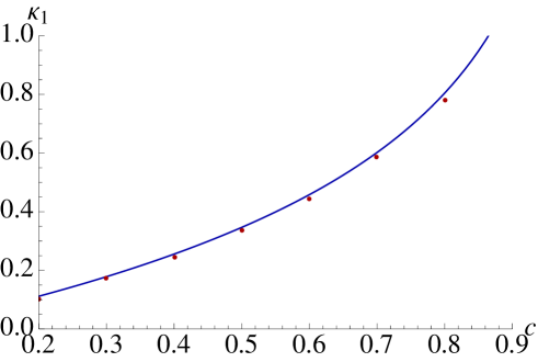
Finally, we numerically check the obtained results (90), (92), and (93). From Fig. 8, we estimate the slopes of the straight lines of logκ𝜅\log\kappa. We denote it by κ1subscript𝜅1\kappa_{1}. We plot κ1subscript𝜅1\kappa_{1} for c=0.2,0.3,,0.8𝑐0.20.30.8c=0.2,0.3,\dots,0.8 in Fig. 10 (red dots) and at the same time we also draw (1/2)log(1c)121𝑐(-1/2)\log(1-c) as a function of c𝑐c (blue line), which is (90). We can see how they coincide.
Refer to caption
Figure 10: κ1subscript𝜅1\kappa_{1} (the exponent in the exponential behavior of κeκ1Lsimilar-to𝜅superscript𝑒subscript𝜅1𝐿\kappa\sim e^{\kappa_{1}L}). We estimated κ1subscript𝜅1\kappa_{1} for c=0.2,0.3,,0.8𝑐0.20.30.8c=0.2,0.3,\dots,0.8 from Fig. 8 for finite L𝐿L and plot those as the red dots. Also, we draw the analytical result 12log(1c)121𝑐-\frac{1}{2}\log(1-c) (blue line) expected in the infinite L𝐿L limit, see (90). The small discrepancy corresponds to finite-size effects, see (96).

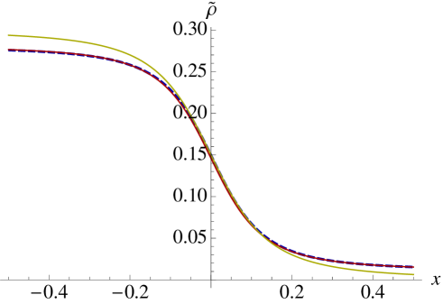
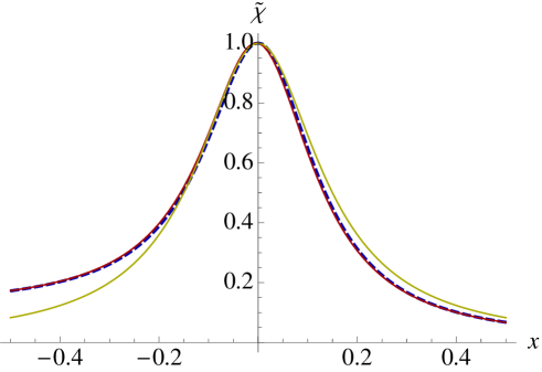
Next, in Fig. 11, we plot the analytical expressions (92), (93) and the corresponding numerical results, as blue dotted lines and red solid lines, respectively.
Refer to caption
Refer to caption
Figure 11: Analytical results for the scaling functions ρ~(x)=ρ(xκ1+sc)~𝜌𝑥𝜌𝑥superscript𝜅1subscript𝑠c\tilde{\rho}(x)=\rho(x\kappa^{-1}+s_{\rm c}) (up) and χ(x)=χ(xκ1+sc)/χ(sc)𝜒𝑥𝜒𝑥superscript𝜅1subscript𝑠c𝜒subscript𝑠c\chi(x)=\chi(x\kappa^{-1}+s_{\rm c})/\chi(s_{\rm c}) (down) for c=0.3𝑐0.3c=0.3 for L=100𝐿100L=100. The solid red lines are the analytical results (92) and (93). The dashed blue lines are the numerical results, which are the same as in Fig. 9. We also plot the infinite-size scaling functions (94) and (95) as the yellow lines, which illustrate the importance of large but finite-size contributions.

The accuracy of the coincidence between the numerical and the analytical results is amazing. On the same figure, we also plot the infinite-size scaling functions (94) and (95) in yellow lines. One can see the deviation between the infinite ones and the finite ones. This indicates that larger system sizes are required to observe the convergence to the infinite-size scaling functions. It is worth mentioning that even for the relatively small system sizes, the finite-size scaling formulæ (92) and (93) show good agreement with the numerical lines. Because the numerical diagonalization becomes harder as the system size becomes larger, the finite-size scaling functions (92) and (93) make the check of the validity of our formulation easier. Furthermore, we also evaluate scsubscript𝑠cs_{\rm c} by using (87). The result is

sc=1/(2Lc(1c))+O(1/L2),subscript𝑠c12𝐿𝑐1𝑐𝑂1superscript𝐿2s_{\rm c}=1/(2Lc(1-c))+O(1/L^{2}), (96)

which is checked numerically in Fig. 1. See Appendix A for the details of the evaluation. This tells us that the upper bound in (24) is actually saturated.

2.7 Scaling function of ψ(s)/s𝜓𝑠𝑠\partial\psi(s)/\partial s

So far, we have focused on the scaling property of ρ(s)𝜌𝑠\rho(s) and χ(s)𝜒𝑠\chi(s). In the similar vein, in this section, we will show the scaling function of ψ(s)/s𝜓𝑠𝑠\partial\psi(s)/\partial s and 2ψ(s)/s2superscript2𝜓𝑠superscript𝑠2\partial^{2}\psi(s)/\partial s^{2}, which correspond to the expectation value and the susceptibility of the activity in the modified system.

First, the expectation value of the activity in the modified system can be calculated as

ψ(s)s=nnPs(n)w(nn)=nPs(n)r(n),𝜓𝑠𝑠subscript𝑛subscriptsuperscript𝑛superscript𝑃𝑠𝑛𝑤𝑛superscript𝑛subscript𝑛superscript𝑃𝑠𝑛𝑟𝑛-\frac{\partial\psi(s)}{\partial s}=\sum_{n}\sum_{n^{\prime}}P^{s}(n)w(n\rightarrow n^{\prime})=\sum_{n}P^{s}(n)r(n), (97)

where r(n)𝑟𝑛r(n) is the escape rate given as (3). Since only n𝑛n and n2superscript𝑛2n^{2} terms constitute r(n)𝑟𝑛r(n), the expectation value of ψ(s)/s𝜓𝑠𝑠\partial\psi(s)/\partial s can be expressed by using only ρ(s)𝜌𝑠\rho(s) and χ(s)𝜒𝑠\chi(s). Indeed, with relations ρ(s)L=neqs𝜌𝑠𝐿superscriptsubscriptdelimited-⟨⟩𝑛eq𝑠\rho(s)L=\left\langle n\right\rangle_{\rm eq}^{s} and n2eqs=Lχ(s)+L2ρ(s)2superscriptsubscriptdelimited-⟨⟩superscript𝑛2eq𝑠𝐿𝜒𝑠superscript𝐿2𝜌superscript𝑠2\left\langle n^{2}\right\rangle_{\rm eq}^{s}=L\chi(s)+L^{2}\rho(s)^{2}, we obtain

ψ(s)s=ρ(s)(Lc+c1)+ρ(s)2L(12c)+(12c)χ(s).𝜓𝑠𝑠𝜌𝑠𝐿𝑐𝑐1𝜌superscript𝑠2𝐿12𝑐12𝑐𝜒𝑠-\frac{\partial\psi(s)}{\partial s}=\rho(s)(Lc+c-1)+\rho(s)^{2}L(1-2c)+(1-2c)\chi(s). (98)

By substituting these ρ(s)𝜌𝑠\rho(s) and χ(s)𝜒𝑠\chi(s) by (68) and (69), changing the variables to x𝑥x, and using (85) and (91), we rewrite it as

ψ(s)s|s=sc+κ1xevaluated-at𝜓𝑠𝑠𝑠subscript𝑠𝑐superscript𝜅1𝑥\displaystyle-\frac{\partial\psi(s)}{\partial s}\big{|}_{s=s_{c}+\kappa^{-1}x}
=12[ρi+ρa](Lc+c1)+12c2L[ρ2i+ρ2a]absent12delimited-[]subscriptdelimited-⟨⟩𝜌𝑖subscriptdelimited-⟨⟩𝜌𝑎𝐿𝑐𝑐112𝑐2𝐿delimited-[]subscriptdelimited-⟨⟩superscript𝜌2𝑖subscriptdelimited-⟨⟩superscript𝜌2𝑎\displaystyle=\frac{1}{2}\left[\left\langle\rho\right\rangle_{i}+\left\langle\rho\right\rangle_{a}\right]\left(Lc+c-1\right)+\frac{1-2c}{2}L\left[\left\langle\rho^{2}\right\rangle_{i}+\left\langle\rho^{2}\right\rangle_{a}\right] (99)
+2x[ρaρi]11+4x2[ρaρi]22𝑥superscriptdelimited-[]delimited-⟨⟩subscript𝜌𝑎subscriptdelimited-⟨⟩𝜌𝑖114superscript𝑥2superscriptdelimited-[]delimited-⟨⟩subscript𝜌𝑎subscriptdelimited-⟨⟩𝜌𝑖2\displaystyle+\frac{2x\left[\left\langle\rho_{a}\right\rangle-\left\langle\rho\right\rangle_{i}\right]^{-1}}{\sqrt{1+4x^{2}\left[\left\langle\rho_{a}\right\rangle-\left\langle\rho\right\rangle_{i}\right]^{-2}}}
×{12[ρiρa](Lc+c1)+12c2L[ρ2iρ2a].}\displaystyle\times\left\{\frac{1}{2}\left[\left\langle\rho\right\rangle_{i}-\left\langle\rho\right\rangle_{a}\right]\left(Lc+c-1\right)+\frac{1-2c}{2}L\left[\left\langle\rho^{2}\right\rangle_{i}-\left\langle\rho^{2}\right\rangle_{a}\right].\right\} (100)

Finally, from this expression, we arrive at the asymptotic expression of ψ(s)/s𝜓𝑠𝑠\partial\psi(s)/\partial s and 2ψ(s)/s2superscript2𝜓𝑠superscript𝑠2\partial^{2}\psi(s)/\partial s^{2} as

limL1Lψ(s)s|s=sc+κ1x=c2(1c)[12xc11+4x2c2],evaluated-atsubscript𝐿1𝐿𝜓𝑠𝑠𝑠subscript𝑠𝑐superscript𝜅1𝑥superscript𝑐21𝑐delimited-[]12𝑥superscript𝑐114superscript𝑥2superscript𝑐2-\lim_{L\rightarrow\infty}\frac{1}{L}\frac{\partial\psi(s)}{\partial s}\bigg{|}_{s=s_{c}+\kappa^{-1}x}=c^{2}(1-c)\left[1-\frac{2xc^{-1}}{\sqrt{1+4x^{2}c^{-2}}}\right], (101)
limL1Lκ2ψ(s)s2|s=sc+κ1x=2c(1c)1(1+4x2c2)3/2.evaluated-atsubscript𝐿1𝐿𝜅superscript2𝜓𝑠superscript𝑠2𝑠subscript𝑠𝑐superscript𝜅1𝑥2𝑐1𝑐1superscript14superscript𝑥2superscript𝑐232\lim_{L\rightarrow\infty}\frac{1}{L\kappa}\frac{\partial^{2}\psi(s)}{\partial s^{2}}\bigg{|}_{s=s_{c}+\kappa^{-1}x}=2c(1-c)\frac{1}{(1+4x^{2}c^{-2})^{3/2}}. (102)

The results of this subsection are directly related to the ones (94) and (95) on the density and variance of occupied sites, and we believe that this connection is generic. The form (101) and (102) provide us a complete description of the fluctuations of the dynamical activity around the transition point, where the fluctuations of the activity are at the origin of the transition itself.

3 Mean-field quantum ferromagnet and the scaling function

In this section, we apply the method in the previous section to a mean-field quantum ferromagnet. We will show that this system has the same scaling functions as (92) and (93). Furthermore, by applying our method to this model, we re-derive a formula that gives the exponent of an exponentially small gap at the quantum phase transition point [22].

3.1 Set up

Let us consider L𝐿L interacting 1/2 spins. The Hilbert space is spanned by the space {|σ|σ=(σ1,,σL){1,+1}N}conditionalket𝜎𝜎subscript𝜎1subscript𝜎𝐿superscript11𝑁\{|\vec{\sigma}\rangle\>|\>\vec{\sigma}=(\sigma_{1},\cdots,\sigma_{L})\in\{-1,+1\}^{N}\}. We denote the Pauli matrices acting on the i𝑖i-th spin by σ^ixsubscriptsuperscript^𝜎𝑥𝑖\hat{\sigma}^{x}_{i}, σ^iysubscriptsuperscript^𝜎𝑦𝑖\hat{\sigma}^{y}_{i}, and σ^izsubscriptsuperscript^𝜎𝑧𝑖\hat{\sigma}^{z}_{i}. These matrices satisfy σiz|σ=σi|σsuperscriptsubscript𝜎𝑖𝑧ket𝜎subscript𝜎𝑖ket𝜎\sigma_{i}^{z}|\vec{\sigma}\rangle=\sigma_{i}|\vec{\sigma}\rangle, σix|σ=|σ(i)superscriptsubscript𝜎𝑖𝑥ket𝜎ketsuperscript𝜎𝑖\sigma_{i}^{x}|\vec{\sigma}\rangle=|\vec{\sigma}^{(i)}\rangle, where σ(i)superscript𝜎𝑖\vec{\sigma}^{(i)} is the configuration in which the i𝑖i-th spin is flipped. The transverse and the longitudinal magnetizations are defined as

m^x=1Li=1Lσ^ix,superscript^𝑚𝑥1𝐿superscriptsubscript𝑖1𝐿superscriptsubscript^𝜎𝑖𝑥\hat{m}^{x}=\frac{1}{L}\sum_{i=1}^{L}\hat{\sigma}_{i}^{x}, (103)
m^z=1Li=1Lσ^iz.superscript^𝑚𝑧1𝐿superscriptsubscript𝑖1𝐿superscriptsubscript^𝜎𝑖𝑧\hat{m}^{z}=\frac{1}{L}\sum_{i=1}^{L}\hat{\sigma}_{i}^{z}. (104)

The Hamiltonian of the mean-field p𝑝p-spin ferromagnet is defined as

H^=L(m^z)pΓLm^x^𝐻𝐿superscriptsuperscript^𝑚𝑧𝑝Γ𝐿superscript^𝑚𝑥\hat{H}=-L(\hat{m}^{z})^{p}-\Gamma L\hat{m}^{x} (105)

There is a phase transition in this model for a special value of ΓΓ\Gamma. It is known that for the p=2𝑝2p=2 (quantum Curie-Weiss model) the transition is second-order, whereas for the p3𝑝3p\geq 3 the transition is first-order. See Ref. [22] for the details of the thermodynamic properties of this model.

Here, we discuss the eigenvalues of the Hamiltonian H^^𝐻\hat{H}. We denote by |ΦketΦ|\Phi\rangle the eigenstate, and by E𝐸E the eigenvalue. We especially focus on the eigenstates, where the interchanges of two spins are permitted. In other words, we focus on the eigenstates that only depend on mz=(1/L)i=1Lσizsuperscript𝑚𝑧1𝐿superscriptsubscript𝑖1𝐿superscriptsubscript𝜎𝑖𝑧m^{z}=(1/L)\sum_{i=1}^{L}\sigma_{i}^{z}:

σ|Φ=Φ(mz).inner-product𝜎ΦΦsuperscript𝑚𝑧\langle\vec{\sigma}|\Phi\rangle=\Phi(m^{z}). (106)

We note that the ground state of H^^𝐻\hat{H} lies in this symmetric subspace. See Ref. [22] for the proof. By multiplying the eigenvalue equation H^|Φ=E|Φ^𝐻ketΦ𝐸ketΦ\hat{H}|\Phi\rangle=E|\Phi\rangle by σ|bra𝜎\langle\vec{\sigma}| from the left, and using (106), we obtain

L(mz)pΦ(mz)ΓL1Li=1L[1+σiz2Φ(mz2/L)+1σiz2Φ(mz+2/L)]𝐿superscriptsuperscript𝑚𝑧𝑝Φsuperscript𝑚𝑧Γ𝐿1𝐿superscriptsubscript𝑖1𝐿delimited-[]1superscriptsubscript𝜎𝑖𝑧2Φsuperscript𝑚𝑧2𝐿1superscriptsubscript𝜎𝑖𝑧2Φsuperscript𝑚𝑧2𝐿\displaystyle-L(m^{z})^{p}\Phi(m^{z})-\Gamma L\frac{1}{L}\sum_{i=1}^{L}\left[\frac{1+\sigma_{i}^{z}}{2}\Phi(m^{z}-2/L)+\frac{1-\sigma_{i}^{z}}{2}\Phi(m^{z}+2/L)\right]
=EΦ(mz),absent𝐸Φsuperscript𝑚𝑧\displaystyle=E\Phi(m^{z}), (107)

which leads to an eigenvalue equation for the symmetric space,

mHm,mΦ(m)=ELΦ(m),subscriptsuperscript𝑚subscript𝐻𝑚superscript𝑚Φsuperscript𝑚𝐸𝐿Φ𝑚\sum_{m^{\prime}\in\mathcal{M}}H_{m,m^{\prime}}\Phi(m^{\prime})=\frac{E}{L}\Phi(m), (108)

where ={1,1+2/L,,12/L,1}112𝐿12𝐿1\mathcal{M}=\{-1,-1+2/L,\cdots,1-2/L,1\} and

Hm,m=(m)pδm,mΓ[1+m2δm2/L,m+1m2δm+2/L,m].subscript𝐻𝑚superscript𝑚superscript𝑚𝑝subscript𝛿𝑚superscript𝑚Γdelimited-[]1𝑚2subscript𝛿𝑚2𝐿superscript𝑚1𝑚2subscript𝛿𝑚2𝐿superscript𝑚H_{m,m^{\prime}}=-(m)^{p}\delta_{m,m^{\prime}}-\Gamma\left[\frac{1+m}{2}\delta_{m-2/L,m^{\prime}}+\frac{1-m}{2}\delta_{m+2/L,m^{\prime}}\right]. (109)

Thanks to the symmetry of the eigenstate, the dimension of the eigenvalue problem is reduced to L+1𝐿1L+1. We note that the matrix Hm,msubscript𝐻𝑚superscript𝑚H_{m,m^{\prime}} is not symmetric although the Hamiltonian H^^𝐻\hat{H} is Hermitian. Here, we define the number of the state p(m)𝑝𝑚p(m) by

p(m)σδmz(σ),m=L!((1+m)L/2)!((1m)L/2)!12L.𝑝𝑚subscript𝜎subscript𝛿superscript𝑚𝑧𝜎𝑚𝐿1𝑚𝐿21𝑚𝐿21superscript2𝐿p(m)\equiv\sum_{\vec{\sigma}}\delta_{m^{z}(\vec{\sigma}),m}=\frac{L!}{((1+m)L/2)!((1-m)L/2)!}\frac{1}{2^{L}}. (110)

With this function, we may calculate the expectation value of a function g(m^z)𝑔superscript^𝑚𝑧g(\hat{m}^{z}) in these symmetric eigenstates from

Φ|g(m^z)|ΦΦ|Φ=mg(m)pΓ(m),quantum-operator-productΦ𝑔superscript^𝑚𝑧Φinner-productΦΦsubscript𝑚𝑔𝑚superscript𝑝Γ𝑚\frac{\langle\Phi|g(\hat{m}^{z})|\Phi\rangle}{\langle\Phi|\Phi\rangle}=\sum_{m}g(m)p^{\Gamma}(m), (111)

where the distribution function pΓ(m)superscript𝑝Γ𝑚p^{\Gamma}(m) is defined as

pΓ(m)=p(m)|Φ(m)|2mp(m)|Φ(m)|2.superscript𝑝Γ𝑚𝑝𝑚superscriptΦ𝑚2subscript𝑚𝑝𝑚superscriptΦ𝑚2p^{\Gamma}(m)=\frac{p(m)|\Phi(m)|^{2}}{\sum_{m}p(m)|\Phi(m)|^{2}}. (112)

Hereafter, we focus on the ground state of the system. The expectation value and the variance of m^zsuperscript^𝑚𝑧\hat{m}^{z} for the ground state is also denoted by m(Γ)𝑚Γm(\Gamma) and σ(Γ)𝜎Γ\sigma(\Gamma), which are calculated as

m(Γ)=mmpΓ(m),𝑚Γsubscript𝑚𝑚superscript𝑝Γ𝑚m(\Gamma)=\sum_{m}mp^{\Gamma}(m), (113)

and

σ(Γ)=Lm(mm(Γ))2pΓ(m).𝜎Γ𝐿subscript𝑚superscript𝑚𝑚Γ2superscript𝑝Γ𝑚\sigma(\Gamma)=L\sum_{m}(m-m(\Gamma))^{2}p^{\Gamma}(m). (114)

The ground state is determined by a variational principle. That is, the ground state energy E𝐸E satisfies

E=min|ΨΨ|H^|ΨΨ|Ψ,𝐸subscriptketΨquantum-operator-productΨ^𝐻Ψinner-productΨΨE=\min_{|\Psi\rangle}\frac{\langle\Psi|\hat{H}|\Psi\rangle}{\langle\Psi|\Psi\rangle}, (115)

where the optimum is reached at the ground state |ΦketΦ|\Phi\rangle. Because the ground state is in the symmetric space [22], we know that |ΦketΦ|\Phi\rangle satisfies (106). This allows us to rewrite (115) as

EL=minΦ~>0mp~(m)mΦ~(m)1Hm,mΦ~(m),𝐸𝐿subscript~Φ0subscript𝑚~𝑝𝑚subscriptsuperscript𝑚~Φsuperscript𝑚1subscript𝐻𝑚superscript𝑚~Φsuperscript𝑚\frac{E}{L}=\min_{\tilde{\Phi}>0}\sum_{m}\tilde{p}(m)\sum_{m^{\prime}}\tilde{\Phi}(m)^{-1}H_{m,m^{\prime}}\tilde{\Phi}(m^{\prime}), (116)

where p~(m)~𝑝𝑚\tilde{p}(m) is defined as

p~(m)=p(m)Φ~(m)2mp(m)Φ~(m)2.~𝑝𝑚𝑝𝑚~Φsuperscript𝑚2subscript𝑚𝑝𝑚~Φsuperscript𝑚2\tilde{p}(m)=\frac{p(m)\tilde{\Phi}(m)^{2}}{\sum_{m}p(m)\tilde{\Phi}(m)^{2}}. (117)

The optimal p~~𝑝\tilde{p} is equal to the ground state distribution function pΓsuperscript𝑝Γp^{\Gamma}. The variational principle has the same structure as (48). The modified distribution for the FA model (49) (or (15)) corresponds to the ground state of the quantum system (117) (or (112)). This correspondence indicates that we might use the same technique as previously to approach the finite-size properties for the quantum system – which we indeed implement in the following subsections.

3.2 Results in infinite-size limit

By assuming the large deviation property for the ground state, we first show a variational principle for the ground state energy in L𝐿L\rightarrow\infty and determine the magnetization and the transverse field corresponding to the first order phase transition.

In the variational principle (48), we assume a large deviation principle for p~(m)~𝑝𝑚\tilde{p}(m): p~(m)eLf~(m)similar-to~𝑝𝑚superscripte𝐿~𝑓𝑚\tilde{p}(m)\sim{\rm e}^{-L\tilde{f}(m)} with a large deviation function f~(m)~𝑓𝑚\tilde{f}(m). This indicates that Φ~(m)~Φ𝑚\tilde{\Phi}(m) also satisfies Φ~eLϕ~(m)/2similar-to~Φsuperscripte𝐿~italic-ϕ𝑚2\tilde{\Phi}\sim{\rm e}^{-L\tilde{\phi}(m)/2} with a large deviation function ϕ~(m)~italic-ϕ𝑚\tilde{\phi}(m). From the large deviation property of p(m)𝑝𝑚p(m), we have the relationship between f~(m)~𝑓𝑚\tilde{f}(m) and ϕ~(m)~italic-ϕ𝑚\tilde{\phi}(m) as

f~(m)=ϕ~(m)+1+m2log(1+m)+1m2log(1m).~𝑓𝑚~italic-ϕ𝑚1𝑚21𝑚1𝑚21𝑚\tilde{f}(m)=\tilde{\phi}(m)+\frac{1+m}{2}\log(1+m)+\frac{1-m}{2}\log(1-m). (118)

The saddle point equation for m𝑚m is f~(m)/m=0~𝑓𝑚𝑚0\partial\tilde{f}(m)/\partial m=0, which leads to

ϕ~(m)m=12log1+m1m.~italic-ϕ𝑚𝑚121𝑚1𝑚\frac{\partial\tilde{\phi}(m)}{\partial m}=\frac{1}{2}\log\frac{1+m}{1-m}. (119)

By evaluating the variational principle (48) with the saddle point approximation, and using (119) in it, we obtain

EL=minm[mpΓ1m2].𝐸𝐿subscript𝑚superscript𝑚𝑝Γ1superscript𝑚2\frac{E}{L}=\min_{m}\left[-m^{p}-\Gamma\sqrt{1-m^{2}}\right]. (120)

This variational formula is well-known. See Ref. [22], for example. By solving this variational formula, we obtain an equation determining the expectation value of the magnetization msuperscript𝑚m^{*}, which is

mΓ=p(m)p11(m)2.xformulae-sequencesuperscript𝑚Γ𝑝superscriptsuperscript𝑚𝑝11superscriptsuperscript𝑚2𝑥m^{*}\Gamma=p\left(m^{*}\right)^{p-1}\sqrt{1-\left(m^{*}\right)^{2}}.x (121)

For p3𝑝3p\geq 3, the system has the first order phase transition [22] with a special value of ΓΓ\Gamma, which we denote ΓcsuperscriptsubscriptΓc\Gamma_{\rm c}^{\infty}. At the transition point, there are two solutions to the variational problem (120), corresponding to the paramagnetic solution mpa=0subscriptsuperscript𝑚pa0m^{\rm pa}_{\infty}=0 and the ferromagnetic solution mfesubscriptsuperscript𝑚fem^{\rm fe}_{\infty}. ΓcsuperscriptsubscriptΓc\Gamma_{\rm c}^{\infty} and mfesubscriptsuperscript𝑚fem^{\rm fe}_{\infty} are determined from the conditions

[mpΓc1m2]|mpa=0=[mpΓc1m2]|m=mfeevaluated-atdelimited-[]superscript𝑚𝑝superscriptsubscriptΓc1superscript𝑚2subscriptsuperscript𝑚pa0evaluated-atdelimited-[]superscript𝑚𝑝superscriptsubscriptΓc1superscript𝑚2𝑚subscriptsuperscript𝑚fe\left[-m^{p}-\Gamma_{\rm c}^{\infty}\sqrt{1-m^{2}}\right]\bigg{|}_{m^{\rm pa}_{\infty}=0}=\left[-m^{p}-\Gamma_{\rm c}^{\infty}\sqrt{1-m^{2}}\right]\bigg{|}_{m=m^{\rm fe}_{\infty}} (122)

and (121) with the replacement of ΓΓ\Gamma and msuperscript𝑚m^{*} by ΓcsuperscriptsubscriptΓc\Gamma_{\rm c}^{\infty} and mfesubscriptsuperscript𝑚fem^{\rm fe}_{\infty}.

In Fig. 12, we plot numerical examples of E/L𝐸𝐿E/L and of the corresponding optimal m𝑚m for p=3𝑝3p=3 obtained from the variational principle (120). At the same time, we also plot the numerical examples of E/L𝐸𝐿E/L, m(Γ)𝑚Γm(\Gamma), and σ(Γ)𝜎Γ\sigma(\Gamma) obtained from the direct diagonalization of the matrix (109) for finite-size systems.
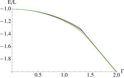
Refer to caption
Refer to caption
Refer to caption
Figure 12: The ground state energy E/L𝐸𝐿E/L (the black line on the upper figure) and the corresponding msuperscript𝑚m^{*} (the black line on the center figure) in the variational principle (120). At the same time, we also plot E/L𝐸𝐿E/L (upper), m(Γ)𝑚Γm(\Gamma) (center) and σ(Γ)𝜎Γ\sigma(\Gamma) (lower) obtained by the numerical diagonalization of the matrix (109). Blue, red, yellow and green lines correspond to L=50,40,30𝐿504030L=50,40,30, and 202020, respectively.

We can see the fist order phase transition around Γc1.3similar-to-or-equalssuperscriptsubscriptΓc1.3\Gamma_{\rm c}^{\infty}\simeq 1.3 in the figure. Also, we can see the finite-size correction of magnetization and susceptibility, which is the next target we consider.

3.3 finite-size structure – scaling functions

Now, we ask how to determine the finite-size structure shown in Fig. 12. For this purpose, we introduce the transition point ΓcLsuperscriptsubscriptΓc𝐿\Gamma_{\rm c}^{L} for the finite-size system as

ΓcL=ArgmaxΓσ(Γ),superscriptsubscriptΓc𝐿subscriptArgmaxΓ𝜎Γ\Gamma_{\rm c}^{L}={\rm Argmax}_{\Gamma}\sigma(\Gamma), (123)

which depends on L𝐿L. Then we define the scaling ratio κ𝜅\kappa by m(ΓcL)/Γ𝑚superscriptsubscriptΓc𝐿Γ-\partial m(\Gamma_{\rm c}^{L})/\partial\Gamma. By using these quantities, we define scaling functions

m~(x)=m(ΓcL+xκ1),~𝑚𝑥𝑚superscriptsubscriptΓc𝐿𝑥superscript𝜅1\tilde{m}(x)=m(\Gamma_{\rm c}^{L}+x\kappa^{-1}), (124)

and

σ~(x)=σ(ΓcL+xκ1)σ(ΓcL).~𝜎𝑥𝜎superscriptsubscriptΓc𝐿𝑥superscript𝜅1𝜎superscriptsubscriptΓc𝐿\tilde{\sigma}(x)=\frac{\sigma(\Gamma_{\rm c}^{L}+x\kappa^{-1})}{\sigma(\Gamma_{\rm c}^{L})}. (125)

The question is how we determine the analytical expression of those scaling functions. For this, we apply the same method as the previous section for the KCM. First, we consider the distribution function pΓ(m)superscript𝑝Γ𝑚p^{\Gamma}(m) at the transition point. We assume that the distribution function is divided into two regions, the paramagnetic region Pp(m)subscript𝑃p𝑚P_{\rm p}(m) and the ferromagnetic region Pf(m)subscript𝑃f𝑚P_{\rm f}(m):

pΓcL(m)=δmmcPp(m)+δm>mcPf(m),superscript𝑝superscriptsubscriptΓc𝐿𝑚subscript𝛿𝑚subscript𝑚csubscript𝑃p𝑚subscript𝛿𝑚subscript𝑚csubscript𝑃f𝑚p^{\Gamma_{\rm c}^{L}}(m)=\delta_{m\leq m_{\rm c}}P_{\rm p}(m)+\delta_{m>m_{\rm c}}P_{\rm f}(m), (126)

where mcsubscript𝑚cm_{\rm c} is the boundary of these two regions, which may be defined as the valley between two peaks for logPp(m)subscript𝑃p𝑚\log P_{\rm p}(m). We note that Pp(m)subscript𝑃p𝑚P_{\rm p}(m) and Pf(m)subscript𝑃f𝑚P_{\rm f}(m) satisfy the condition of first-order phase transitions

mmcPp(m)=m>mcPf(m)=1/2.subscript𝑚subscript𝑚csubscript𝑃p𝑚subscript𝑚subscript𝑚csubscript𝑃f𝑚12\sum_{m\leq m_{\rm c}}P_{\rm p}(m)=\sum_{m>m_{\rm c}}P_{\rm f}(m)=1/2. (127)

Next, for the region around ΓcLsuperscriptsubscriptΓc𝐿\Gamma_{\rm c}^{L}, we assume that pΓsuperscript𝑝Γp^{\Gamma} is written as

pΓ(m)=(1+a(Γ))δmmcPp(m)+(1a(Γ))δm>mcPf(m),superscript𝑝Γ𝑚1superscript𝑎Γsubscript𝛿𝑚subscript𝑚csubscript𝑃p𝑚1superscript𝑎Γsubscript𝛿𝑚subscript𝑚csubscript𝑃f𝑚p^{\Gamma}(m)=(1+a^{*}(\Gamma))\delta_{m\leq m_{\rm c}}P_{\rm p}(m)+(1-a^{*}(\Gamma))\delta_{m>m_{\rm c}}P_{\rm f}(m), (128)

where a(Γ)superscript𝑎Γa^{*}(\Gamma) is a mixing function of ΓΓ\Gamma. We note that the normalization condition is satisfied due to (127). From the distribution function, we can calculate m(Γ)𝑚Γm(\Gamma), σ(Γ)𝜎Γ\sigma(\Gamma) as

m(Γ)=mp2[1+a(Γ)]+mf2[1a(Γ)],𝑚Γsubscriptdelimited-⟨⟩𝑚p2delimited-[]1superscript𝑎Γsubscriptdelimited-⟨⟩𝑚f2delimited-[]1superscript𝑎Γm(\Gamma)=\frac{\left\langle m\right\rangle_{\rm p}}{2}\left[1+a^{*}(\Gamma)\right]+\frac{\left\langle m\right\rangle_{\rm f}}{2}\left[1-a^{*}(\Gamma)\right], (129)
σ(Γ)=L{m2p2[1+a(Γ)]+m2f2[1a(Γ)]m(Γ)2},𝜎Γ𝐿subscriptdelimited-⟨⟩superscript𝑚2p2delimited-[]1superscript𝑎Γsubscriptdelimited-⟨⟩superscript𝑚2f2delimited-[]1superscript𝑎Γ𝑚superscriptΓ2\sigma(\Gamma)=L\left\{\frac{\left\langle m^{2}\right\rangle_{\rm p}}{2}\left[1+a^{*}(\Gamma)\right]+\frac{\left\langle m^{2}\right\rangle_{\rm f}}{2}\left[1-a^{*}(\Gamma)\right]-m(\Gamma)^{2}\right\}, (130)

where psubscriptp\left\langle\ \right\rangle_{\rm p} and fsubscriptf\left\langle\ \right\rangle_{\rm f} are the expectation values in the paramagnetic phase and the ferromagnetic phase, respectively, which are defined as gp=2mmcPp(m)g(m)subscriptdelimited-⟨⟩𝑔p2subscript𝑚subscript𝑚csubscript𝑃p𝑚𝑔𝑚\left\langle g\right\rangle_{\rm p}=2\sum_{m\leq m_{\rm c}}P_{\rm p}(m)g(m) and gf=2m>mcPf(m)g(m)subscriptdelimited-⟨⟩𝑔f2subscript𝑚subscript𝑚csubscript𝑃f𝑚𝑔𝑚\left\langle g\right\rangle_{\rm f}=2\sum_{m>m_{\rm c}}P_{\rm f}(m)g(m). For the determination of a(Γ)superscript𝑎Γa^{*}(\Gamma), we use the variational principle (116). Indeed, from (128) with (112), we have Φ(m)Φ𝑚\Phi(m). By substituting the obtained Φ(m)|a(Γ)=aevaluated-atΦ𝑚superscript𝑎Γ𝑎\Phi(m)|_{a^{*}(\Gamma)=a} and pΓ(m)|a(Γ)=aevaluated-atsuperscript𝑝Γ𝑚superscript𝑎Γ𝑎p^{\Gamma}(m)|_{a^{*}(\Gamma)=a} into the variational functional of (116) and maximizing it with respect to a𝑎a, we obtain the optimal asuperscript𝑎a^{*}, which corresponds to a(Γ)superscript𝑎Γa^{*}(\Gamma). The result is

a(Γ)=x[mpmf]11+4x2[mpmf]2+O(κ1).superscript𝑎Γ𝑥superscriptdelimited-[]subscriptdelimited-⟨⟩𝑚psubscriptdelimited-⟨⟩𝑚f114superscript𝑥2superscriptdelimited-[]subscriptdelimited-⟨⟩𝑚psubscriptdelimited-⟨⟩𝑚f2𝑂superscript𝜅1a^{*}(\Gamma)=\frac{x\left[\left\langle m\right\rangle_{\rm p}-\left\langle m\right\rangle_{\rm f}\right]^{-1}}{\sqrt{1+4x^{2}\left[\left\langle m\right\rangle_{\rm p}-\left\langle m\right\rangle_{\rm f}\right]^{-2}}}+O(\kappa^{-1}). (131)

with x=κ(ΓΓc)𝑥𝜅ΓsubscriptΓcx=\kappa(\Gamma-\Gamma_{\rm c}). Combining it with (129) and (130), we obtain

m~(x)=12[mp+mf2x1+4x2[mpmf]2],~𝑚𝑥12delimited-[]subscriptdelimited-⟨⟩𝑚psubscriptdelimited-⟨⟩𝑚f2𝑥14superscript𝑥2superscriptdelimited-[]subscriptdelimited-⟨⟩𝑚psubscriptdelimited-⟨⟩𝑚f2\tilde{m}(x)=\frac{1}{2}\left[\left\langle m\right\rangle_{\rm p}+\left\langle m\right\rangle_{\rm f}-\frac{2x}{\sqrt{1+4x^{2}\left[\left\langle m\right\rangle_{\rm p}-\left\langle m\right\rangle_{\rm f}\right]^{-2}}}\right], (132)
σ~(x)=~𝜎𝑥absent\displaystyle\tilde{\sigma}(x)=
1C[m2p+m2f2x[m2pm2f][mpmf]11+4x2[mpmf]22m~(x)2],1𝐶delimited-[]subscriptdelimited-⟨⟩superscript𝑚2psubscriptdelimited-⟨⟩superscript𝑚2f2𝑥delimited-[]subscriptdelimited-⟨⟩superscript𝑚2psubscriptdelimited-⟨⟩superscript𝑚2fsuperscriptdelimited-[]subscriptdelimited-⟨⟩𝑚psubscriptdelimited-⟨⟩𝑚f114superscript𝑥2superscriptdelimited-[]subscriptdelimited-⟨⟩𝑚psubscriptdelimited-⟨⟩𝑚f22~𝑚superscript𝑥2\displaystyle\;\frac{1}{C}\left[\left\langle m^{2}\right\rangle_{\rm p}+\left\langle m^{2}\right\rangle_{\rm f}-\frac{2x\left[\left\langle m^{2}\right\rangle_{\rm p}-\left\langle m^{2}\right\rangle_{\rm f}\right]\left[\left\langle m\right\rangle_{\rm p}-\left\langle m\right\rangle_{\rm f}\right]^{-1}}{\sqrt{1+4x^{2}\left[\left\langle m\right\rangle_{\rm p}-\left\langle m\right\rangle_{\rm f}\right]^{-2}}}-2\tilde{m}(x)^{2}\right], (133)

where C𝐶C is

C=m2p+m2f2m~(0)2.𝐶subscriptdelimited-⟨⟩superscript𝑚2psubscriptdelimited-⟨⟩superscript𝑚2f2~𝑚superscript02C=\left\langle m^{2}\right\rangle_{\rm p}+\left\langle m^{2}\right\rangle_{\rm f}-2\tilde{m}(0)^{2}. (134)

These expressions are equivalent to the relations (92) and (93) that we obtained in our study of the KCM. Noticing that limLmp=limLm2p=0subscript𝐿subscriptdelimited-⟨⟩𝑚psubscript𝐿subscriptdelimited-⟨⟩superscript𝑚2p0\lim_{L\rightarrow\infty}\left\langle m\right\rangle_{\rm p}=\lim_{L\rightarrow\infty}\left\langle m^{2}\right\rangle_{\rm p}=0, limLmf=mfesubscript𝐿subscriptdelimited-⟨⟩𝑚fsuperscriptsubscript𝑚fe\lim_{L\rightarrow\infty}\left\langle m\right\rangle_{\rm f}=m_{\infty}^{\rm fe}, and limLm2f=(mfe)2subscript𝐿subscriptdelimited-⟨⟩superscript𝑚2fsuperscriptsuperscriptsubscript𝑚fe2\lim_{L\rightarrow\infty}\left\langle m^{2}\right\rangle_{\rm f}=(m_{\infty}^{\rm fe})^{2}, we also obtain the infinite-size scaling functions:

m~(x)=limLm~(x)=12[mfe2x1+4x2(mfe)2],subscript~𝑚𝑥subscript𝐿~𝑚𝑥12delimited-[]superscriptsubscript𝑚fe2𝑥14superscript𝑥2superscriptsuperscriptsubscript𝑚fe2\tilde{m}_{\infty}(x)=\lim_{L\rightarrow\infty}\tilde{m}(x)=\frac{1}{2}\left[m_{\infty}^{\rm fe}-\frac{2x}{\sqrt{1+4x^{2}(m_{\infty}^{\rm fe})^{-2}}}\right], (135)
σ~(x)=limLσ~(x)=(mfe)2(mfe)2+4x2,subscript~𝜎𝑥subscript𝐿~𝜎𝑥superscriptsuperscriptsubscript𝑚fe2superscriptsuperscriptsubscript𝑚fe24superscript𝑥2\tilde{\sigma}_{\infty}(x)=\lim_{L\rightarrow\infty}\tilde{\sigma}(x)=\frac{(m_{\infty}^{\rm fe})^{2}}{(m_{\infty}^{\rm fe})^{2}+4x^{2}}, (136)

which correspond to (94) and (95). We check the obtained results in Fig. 13, from which one can see that (132) and (133) (solid red lines) show good agreement with the numerical results from direct diagonalization (blue dotted lines). As the same as the previous section, we also note that large system sizes are required to observe the convergence to the infinite-size scaling functions (135) and (136).
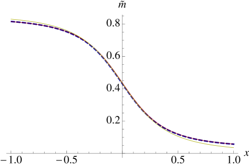
Refer to caption
Refer to caption
Figure 13: The scaling functions m~(x)~𝑚𝑥\tilde{m}(x) (up) and σ~(x)~𝜎𝑥\tilde{\sigma}(x) (down) for p=3𝑝3p=3 and L=100𝐿100L=100. The solid red lines are the analytical results (132) and (133). The dashed blue lines are the numerical results obtained from the direct diagonalization of (109) for each x𝑥x (or Γ)\Gamma). For (132) and (133), we need the distribution function PP(m)subscript𝑃P𝑚P_{\rm P}(m) and Pf(m)subscript𝑃f𝑚P_{\rm f}(m) at Γ=ΓcLΓsuperscriptsubscriptΓc𝐿\Gamma=\Gamma_{\rm c}^{L}. To obtain the distribution function, here, we evaluated the corresponding eigenvector for x=0𝑥0x=0 (or Γ=ΓcLΓsuperscriptsubscriptΓc𝐿\Gamma=\Gamma_{\rm c}^{L}), numerically. We also plot the infinite-size scaling functions (135) and (136) as solid yellow lines.

3.4 finite-size structure – scaling factor and exponentially small gap

Finally, we derive the exponent of the scaling factor κ𝜅\kappa, which is equivalent to the exponentially small gap derived in [22].

We first define the free energy for the ground state at the transition point ΓcsuperscriptsubscriptΓc\Gamma_{\rm c}^{\infty} by

fΓc(m)=limL1LlogpΓc(m).subscript𝑓superscriptsubscriptΓc𝑚subscript𝐿1𝐿superscript𝑝superscriptsubscriptΓc𝑚f_{\Gamma_{\rm c}^{\infty}}(m)=-\lim_{L\rightarrow\infty}\frac{1}{L}\log p^{\Gamma_{\rm c}^{\infty}}(m). (137)

Then, using the same argument as for (90), we obtain the exponent κ𝜅\kappa

limL1Llogκ=fΓc(mc),subscript𝐿1𝐿𝜅subscript𝑓superscriptsubscriptΓcsuperscriptsubscript𝑚c\lim_{L\rightarrow\infty}\frac{1}{L}\log\kappa=f_{\Gamma_{\rm c}^{\infty}}(m_{\rm c}^{\infty}), (138)

where mc=limLmcsuperscriptsubscript𝑚csubscript𝐿subscript𝑚cm_{\rm c}^{\infty}=\lim_{L\rightarrow\infty}m_{\rm c} represents the connecting point between the paramagnetic and the ferromagnetic regions in the infinite system size limit.

Next, we determine the free energy. We start from the ground state of the eigenvalue equation for Γ=ΓcΓsuperscriptsubscriptΓc\Gamma=\Gamma_{\rm c}^{\infty},

mpΓc[1+m2Φ(m2/L)Φ(m)+1m2Φ(m+2/L)Φ(m)]=EL,superscript𝑚𝑝superscriptsubscriptΓcdelimited-[]1𝑚2Φ𝑚2𝐿Φ𝑚1𝑚2Φ𝑚2𝐿Φ𝑚𝐸𝐿-m^{p}-\Gamma_{\rm c}^{\infty}\left[\frac{1+m}{2}\frac{\Phi(m-2/L)}{\Phi(m)}+\frac{1-m}{2}\frac{\Phi(m+2/L)}{\Phi(m)}\right]=\frac{E}{L}, (139)

which is obtained from (108). Now, we assume a large deviation principle. That is, we set Φ(m)=e(L/2)ϕ(m)Φ𝑚superscript𝑒𝐿2italic-ϕ𝑚\Phi(m)=e^{-(L/2)\phi(m)} in (139). The leading term of (139) is

mpΓc[1+m2eϕ/m+1m2eϕ/m]=ec,superscript𝑚𝑝superscriptsubscriptΓcdelimited-[]1𝑚2superscript𝑒italic-ϕ𝑚1𝑚2superscript𝑒italic-ϕ𝑚subscriptsuperscript𝑒c-m^{p}-\Gamma_{\rm c}^{\infty}\left[\frac{1+m}{2}e^{\partial\phi/\partial m}+\frac{1-m}{2}e^{-\partial\phi/\partial m}\right]=e^{\infty}_{\rm c}, (140)

where we define limLE/L|Γ=Γcecevaluated-atsubscript𝐿𝐸𝐿ΓsuperscriptsubscriptΓcsubscriptsuperscript𝑒c\lim_{L\rightarrow\infty}E/L|_{\Gamma=\Gamma_{\rm c}^{\infty}}\equiv e^{\infty}_{\rm c}. By solving this equation, we obtain two solutions for the expression ϕ(m)/mitalic-ϕ𝑚𝑚\partial\phi(m)/\partial m as

ϕ(m)+const.italic-ϕ𝑚const\displaystyle\phi(m)+{\rm const.}
=ϕ±(m)absentsubscriptitalic-ϕplus-or-minus𝑚\displaystyle=\phi_{\pm}(m)
0m𝑑m~log[m~p+ec(1+m~)Γc±(m~p+ec(1+m~)Γc)21m~1+m~]absentsuperscriptsubscript0𝑚differential-d~𝑚plus-or-minussuperscript~𝑚𝑝subscriptsuperscript𝑒c1~𝑚superscriptsubscriptΓcsuperscriptsuperscript~𝑚𝑝subscriptsuperscript𝑒c1~𝑚superscriptsubscriptΓc21~𝑚1~𝑚\displaystyle\equiv\int_{0}^{m}d\tilde{m}\log\left[-\frac{\tilde{m}^{p}+e^{\infty}_{\rm c}}{(1+\tilde{m})\Gamma_{\rm c}^{\infty}}\pm\sqrt{\left(\frac{\tilde{m}^{p}+e^{\infty}_{\rm c}}{(1+\tilde{m})\Gamma_{\rm c}^{\infty}}\right)^{2}-\frac{1-\tilde{m}}{1+\tilde{m}}}\right] (141)

By using these two functions, we also define free energies as

f±(m)subscript𝑓plus-or-minus𝑚\displaystyle f_{\pm}(m) ϕ±(m)+1+m2log(1+m)+1m2log(1m)absentsubscriptitalic-ϕplus-or-minus𝑚1𝑚21𝑚1𝑚21𝑚\displaystyle\equiv\phi_{\pm}(m)+\frac{1+m}{2}\log(1+m)+\frac{1-m}{2}\log(1-m) (142)
=0m𝑑m~log[m~p+ec1m~2Γc±(m~p+ec1m~2Γc)21]absentsuperscriptsubscript0𝑚differential-d~𝑚plus-or-minussuperscript~𝑚𝑝subscriptsuperscript𝑒c1superscript~𝑚2superscriptsubscriptΓcsuperscriptsuperscript~𝑚𝑝subscriptsuperscript𝑒c1superscript~𝑚2superscriptsubscriptΓc21\displaystyle=\int_{0}^{m}d\tilde{m}\log\left[-\frac{\tilde{m}^{p}+e^{\infty}_{\rm c}}{\sqrt{1-\tilde{m}^{2}}\Gamma_{\rm c}^{\infty}}\pm\sqrt{\left(\frac{\tilde{m}^{p}+e^{\infty}_{\rm c}}{\sqrt{1-\tilde{m}^{2}}\Gamma_{\rm c}^{\infty}}\right)^{2}-1}\right]

The free energy fΓc(m)subscript𝑓superscriptsubscriptΓc𝑚f_{\Gamma_{\rm c}^{\infty}}(m) is given as the combination of f+(m)subscript𝑓𝑚f_{+}(m) and f(m)subscript𝑓𝑚f_{-}(m). Here, we notice

fΓc(0)=fΓc(mfe)=0.subscript𝑓superscriptsubscriptΓc0subscript𝑓superscriptsubscriptΓcsuperscriptsubscript𝑚fe0f_{\Gamma_{\rm c}^{\infty}}(0)=f_{\Gamma_{\rm c}^{\infty}}(m_{\rm fe}^{\infty})=0. (143)

Also, we can easily check

f+(m)m|m=0>0evaluated-atsubscript𝑓𝑚𝑚𝑚00\frac{\partial f_{+}(m)}{\partial m}\bigg{|}_{m=0}>0 (144)
f(m)m|m=0<0.evaluated-atsubscript𝑓𝑚𝑚𝑚00\frac{\partial f_{-}(m)}{\partial m}\bigg{|}_{m=0}<0. (145)

From (143), (144) and (145), we can construct the free energy fΓc(m)subscript𝑓superscriptsubscriptΓc𝑚f_{\Gamma_{\rm c}^{\infty}}(m) as

fΓc(m)=f+(m)subscript𝑓superscriptsubscriptΓc𝑚subscript𝑓𝑚f_{\Gamma_{\rm c}^{\infty}}(m)=f_{+}(m) (146)

for mmc𝑚superscriptsubscript𝑚cm\leq m_{\rm c}^{\infty}

fΓc(m)=f(m)+const.subscript𝑓superscriptsubscriptΓc𝑚subscript𝑓𝑚constf_{\Gamma_{\rm c}^{\infty}}(m)=f_{-}(m)+\rm const. (147)

for m>mc𝑚superscriptsubscript𝑚cm>m_{\rm c}^{\infty}. The constant and mcsuperscriptsubscript𝑚cm_{\rm c}^{\infty} is determined from (143) and the continuity condition

limmmc+0fΓc(m)=limmmc0fΓc(m).subscript𝑚subscript𝑚c0subscript𝑓superscriptsubscriptΓc𝑚subscript𝑚subscript𝑚c0subscript𝑓superscriptsubscriptΓc𝑚\lim_{m\rightarrow m_{\rm c}+0}f_{\Gamma_{\rm c}^{\infty}}(m)=\lim_{m\rightarrow m_{\rm c}-0}f_{\Gamma_{\rm c}^{\infty}}(m). (148)

By using the parameters ΓcsuperscriptsubscriptΓc\Gamma_{\rm c}^{\infty}, ecsubscriptsuperscript𝑒ce^{\infty}_{\rm c}, and mfesuperscriptsubscript𝑚fem_{\rm fe}^{\infty} obtained from (120), (121) and (122), we can calculate the gap given by (138) in principle. Here, however, by using a relation

f+(m)=f(m)+const.,subscript𝑓𝑚subscript𝑓𝑚constf_{+}(m)=-f_{-}(m)+\rm const., (149)

which can be derived from the direct substitution, we will show that the gap can be expressed as a simple formula. Indeed, from this relation, we can derive

f+(mc)=12f+(mfe).subscript𝑓superscriptsubscript𝑚c12subscript𝑓superscriptsubscript𝑚fef_{+}(m_{\rm c}^{\infty})=\frac{1}{2}f_{+}(m_{\rm fe}^{\infty}). (150)

Thus, we arrive at

limL1Llogκsubscript𝐿1𝐿𝜅\displaystyle\lim_{L\rightarrow\infty}\frac{1}{L}\log\kappa
=12f+(mfe)absent12subscript𝑓superscriptsubscript𝑚fe\displaystyle=\frac{1}{2}f_{+}(m_{\rm fe}^{\infty})
=0mfe𝑑mlog[mp+ec1m2Γc+(mp+ec1m2Γc)21]absentsuperscriptsubscript0superscriptsubscript𝑚fedifferential-d𝑚superscript𝑚𝑝subscriptsuperscript𝑒c1superscript𝑚2superscriptsubscriptΓcsuperscriptsuperscript𝑚𝑝subscriptsuperscript𝑒c1superscript𝑚2superscriptsubscriptΓc21\displaystyle=\int_{0}^{m_{\rm fe}^{\infty}}dm\log\left[-\frac{m^{p}+e^{\infty}_{\rm c}}{\sqrt{1-m^{2}}\Gamma_{\rm c}^{\infty}}+\sqrt{\left(\frac{m^{p}+e^{\infty}_{\rm c}}{\sqrt{1-m^{2}}\Gamma_{\rm c}^{\infty}}\right)^{2}-1}\right] (151)

This formula is equivalent to the formula obtained by Bapst and Semerjian, Eq. (62) in Ref. [22]. In order to see the equivalence, we just use a basic mathematical fact that the following equations coshx=A𝑥𝐴\cosh x=A and ex=A±A21superscript𝑒𝑥plus-or-minus𝐴superscript𝐴21e^{x}=A\pm\sqrt{A^{2}-1} are equivalent.

4 Conclusions

Our goal in this work was to identify the characteristic features of finite-size scaling at a first-order dynamical transition, as can be found generically in KCMs. As we have shown, these are akin to characteristic features of a first-order quantum transition. We have been able, in particular, to determine in an explicit fashion the scaling variables and the scaling functions governing the variation of the order parameter across the transition. For the particular mean-field KCM that we have been considering here, a precise characterization of a size-dependent critical point was provided and the finite-size rounding off of the transition was fully captured by our study. Interestingly, the phenomenology of our dynamical transition – which is identical to that of quantum transitions, but now capturing finite-size scaling – also agrees with that of classical first order transitions, as our variational formulation in terms of the mixing function a(s)superscript𝑎𝑠a^{*}(s) confirms.

We also note that after the submission of our work, Campostrini and collaborators presented results in a recent preprint [31] on the finite-size scaling of first-order quantum phase transition. Close to the critical point, scaling functions for their order parameter take the same form as presented in our approach, with a derivation based on a two-level effective model. Further connections between our work and this approach (and also with the two-level effective model of [21] used for an instantonic computation of the gap) are worth studying.

The mean-field version being now fully understood, a more challenging program awaits ahead of us. Finite-dimensional systems of course display a richer phenomenology [13] with, for instance, the existence of surface tension and nucleating droplets. It is in principle possible to extend our analysis for the density large deviation function to a space varying field, by means of field theoretic methods à la Doi-Peliti [32, 33], for example. When studying dynamical transitions, some authors [10] work at fixed system size, but they perform a finite time analysis (which would be mimicked by a finite temperature analysis in quantum phase transition). It would certainly be of interest to quantify in a similar way finite-time corrections, though the phase transition itself is indeed a collective effect captured only at large N𝑁N. These issues are currently under investigation.

Acknowledgments – we would like to thank an anonymous referee for pointing out an error in a previous version of subsection 2.2. This work was supported by JSPS Core-to-Core program “Non-equilibrium dynamics of soft matter and information” and by the “LaBS” PEPS CNRS project.

A Determination of scsubscript𝑠𝑐s_{c}

In this appendix, we derive sc=1/(2Lc(1c))+O(1/L2)subscript𝑠c12𝐿𝑐1𝑐𝑂1superscript𝐿2s_{\rm c}=1/(2Lc(1-c))+O(1/L^{2}). We evaluate (87) up to O(1/L)𝑂1𝐿O(1/L) by using the explicit expressions of r𝑟r, r~isubscript~𝑟i\tilde{r}_{\rm i}, and r~asubscript~𝑟a\tilde{r}_{\rm a}. From a saddle point approximation, we rewrite the left-hand side of (87) as

1L(r~iescr)|n=1+O(1/L2)=cLesceLfi(2/L)/2eLfi(1/L)/2cL+O(1/L2).evaluated-at1𝐿subscript~𝑟isuperscriptesubscript𝑠c𝑟𝑛1𝑂1superscript𝐿2𝑐𝐿superscriptesubscript𝑠csuperscripte𝐿subscript𝑓i2𝐿2superscripte𝐿subscript𝑓i1𝐿2𝑐𝐿𝑂1superscript𝐿2\frac{1}{L}\left(\tilde{r}_{\rm i}{\rm e}^{-s_{\rm c}}-r\right)\Big{|}_{n=1}+O(1/L^{2})=\frac{c}{L}{\rm e}^{-s_{\rm c}}\frac{{\rm e}^{-Lf_{\rm i}(2/L)/2}}{{\rm e}^{-Lf_{\rm i}(1/L)/2}}-\frac{c}{L}+O(1/L^{2}). (152)

Here, the first term is O(1/L2)𝑂1superscript𝐿2O(1/L^{2}) since

eLfi(2/L)/2eLfi(1/L)/2=O(1/L).superscripte𝐿subscript𝑓i2𝐿2superscripte𝐿subscript𝑓i1𝐿2𝑂1𝐿\frac{{\rm e}^{-Lf_{\rm i}(2/L)/2}}{{\rm e}^{-Lf_{\rm i}(1/L)/2}}=O(1/L). (153)

Thus, the left-hand side of (87) is c/L+O(1/L2)𝑐𝐿𝑂1superscript𝐿2-c/L+O(1/L^{2}). On the other hand, the right-hand side of (87) is evaluated by saddle point approximation as

1L(r~aescr)|n=Lc+O(1/L2)evaluated-at1𝐿subscript~𝑟asuperscriptesubscript𝑠c𝑟𝑛𝐿𝑐𝑂1superscript𝐿2\displaystyle\frac{1}{L}\left(\tilde{r}_{\rm a}{\rm e}^{-s_{\rm c}}-r\right)\Big{|}_{n=Lc}+O(1/L^{2})
=c2(1c)[e12fa(ρ)ρ|ρ=csc+e12fa(ρ)ρ|ρ=csc2]+O(1/L2).absentsuperscript𝑐21𝑐delimited-[]superscripteevaluated-at12subscript𝑓𝑎𝜌𝜌𝜌𝑐subscript𝑠csuperscripteevaluated-at12subscript𝑓𝑎𝜌𝜌𝜌𝑐subscript𝑠c2𝑂1superscript𝐿2\displaystyle=c^{2}(1-c)\left[{\rm e}^{-\frac{1}{2}\frac{\partial f_{a}(\rho)}{\partial\rho}|_{\rho=c}-s_{\rm c}}+{\rm e}^{\frac{1}{2}\frac{\partial f_{a}(\rho)}{\partial\rho}|_{\rho=c}-s_{\rm c}}-2\right]+O(1/L^{2}). (154)

By noticing that fa(ρ)/ρ|ρ=cevaluated-atsubscript𝑓𝑎𝜌𝜌𝜌𝑐\partial f_{a}(\rho)/\partial\rho|_{\rho=c} and scsubscript𝑠cs_{\rm c} are O(1/L)𝑂1𝐿O(1/L), we rewrite (154) as

2scc2(1c)+O(1/L2).2subscript𝑠csuperscript𝑐21𝑐𝑂1superscript𝐿2-2s_{\rm c}\,c^{2}(1-c)+O(1/L^{2}). (155)

Therefore, by equating the left-hand side of (87) to the right-hand side of (87), we arrive at

sc=12Lc(1c)+O(1/L2).subscript𝑠c12𝐿𝑐1𝑐𝑂1superscript𝐿2s_{\rm c}=\frac{1}{2Lc(1-c)}+O(1/L^{2}). (156)

B Finite-size corrections to the free energy difference

In this appendix, we derive the finite-size correction Δfsc(1)(ρ)Δsuperscriptsubscript𝑓subscript𝑠c1𝜌\Delta f_{s_{\rm c}}^{(1)}(\rho) given in (39) and (40). We first focus on the region ρ>ρcL𝜌superscriptsubscript𝜌c𝐿\rho>\rho_{\rm c}^{L}. From (26) with (38), we find that ΦL(n)subscriptΦL𝑛\Phi_{\rm L}(n) doesn’t satisfy the large deviation principle. Then, we define Φ~L(ρ)=ΦL(ρL)subscript~ΦL𝜌subscriptΦL𝜌𝐿\tilde{\Phi}_{\rm L}(\rho)=\Phi_{\rm L}(\rho L). From the fact ΦL(n)subscriptΦL𝑛\Phi_{\rm L}(n) doesn’t satisfy the large deviation scaling, we can assume Φ~L(ρ)subscript~ΦL𝜌\tilde{\Phi}_{\rm L}(\rho) is differentiable:

Φ~L(ρ±1/L)=Φ~L(ρ)±Φ~Lρ1L+O(1/L2).subscript~ΦLplus-or-minus𝜌1𝐿plus-or-minussubscript~ΦL𝜌subscript~ΦL𝜌1𝐿𝑂1superscript𝐿2\tilde{\Phi}_{\rm L}(\rho\pm 1/L)=\tilde{\Phi}_{\rm L}(\rho)\pm\frac{\partial\tilde{\Phi}_{\rm L}}{\partial\rho}\frac{1}{L}+O(1/L^{2}). (157)

By rewriting the left-hand side of (26) by using this scaling, we obtain a differential equation for determining Φ~L(ρ)subscript~ΦL𝜌\tilde{\Phi}_{\rm L}(\rho).

Φ~L(ρ){s~cρ[c+(12c)ρ]+c}+Φ~L(ρ)ρρ(cρ)+O(1/L2)=0,subscript~ΦL𝜌subscript~𝑠c𝜌delimited-[]𝑐12𝑐𝜌𝑐subscript~ΦL𝜌𝜌𝜌𝑐𝜌𝑂1superscript𝐿20\tilde{\Phi}_{\rm L}(\rho)\left\{-\tilde{s}_{\rm c}\rho\left[c+(1-2c)\rho\right]+c\right\}+\frac{\partial\tilde{\Phi}_{\rm L}(\rho)}{\partial\rho}\rho(c-\rho)+O(1/L^{2})=0, (158)

where we defined s~csLsubscript~𝑠𝑐𝑠𝐿\tilde{s}_{c}\equiv sL. By solving this differential equation, we obtain

2logΦ~L(ρ)2subscript~ΦL𝜌\displaystyle-2\log\tilde{\Phi}_{\rm L}(\rho)
=2[s~cρ(2c1)logρ+(s~c2c(1c)+1)log|cρ|]+const.absent2delimited-[]subscript~𝑠c𝜌2𝑐1𝜌subscript~𝑠c2𝑐1𝑐1𝑐𝜌const\displaystyle=-2\left[\tilde{s}_{\rm c}\rho(2c-1)-\log\rho+(-\tilde{s}_{\rm c}2c(1-c)+1)\log|c-\rho|\right]+\rm const. (159)

Finally with a relation s~c=1/(2c(1c))+O(1/L)subscript~𝑠c12𝑐1𝑐𝑂1𝐿\tilde{s}_{\rm c}=1/(2c(1-c))+O(1/L), we can omit the last term. The result leads to

2logΦ~L(ρ)=Δfsc(1)(ρ)=2[ρ(2c1)2c(1c)logρ]+const.2subscript~ΦL𝜌Δsuperscriptsubscript𝑓subscript𝑠c1𝜌2delimited-[]𝜌2𝑐12𝑐1𝑐𝜌const\displaystyle-2\log\tilde{\Phi}_{\rm L}(\rho)=\Delta f_{s_{\rm c}}^{(1)}(\rho)=-2\left[\frac{\rho(2c-1)}{2c(1-c)}-\log\rho\right]+\rm const. (160)

Next, we focus on the region ρρcL𝜌superscriptsubscript𝜌c𝐿\rho\leq\rho_{\rm c}^{L}. By using the explicit expression of ΔfscΔsubscript𝑓subscript𝑠c\Delta f_{s_{\rm c}} in this region, we evaluate the equation (26) up to O(1/L)𝑂1𝐿O(1/L). First, ΦL(n+1)/ΦL(n)subscriptΦL𝑛1subscriptΦL𝑛\Phi_{\rm L}(n+1)/\Phi_{\rm L}(n) is evaluated as

ΦL(n+1)ΦL(n)subscriptΦL𝑛1subscriptΦL𝑛\displaystyle\frac{\Phi_{\rm L}(n+1)}{\Phi_{\rm L}(n)} =efe/ρ+1/(2L)2fe/ρ21/(2L)Δfsc(1)/ρabsentsuperscript𝑒subscript𝑓e𝜌12𝐿superscript2subscript𝑓esuperscript𝜌212𝐿Δsuperscriptsubscript𝑓subscript𝑠c1𝜌\displaystyle=e^{\partial f_{\rm e}/\partial\rho+1/(2L)\partial^{2}f_{\rm e}/\partial\rho^{2}-1/(2L)\partial\Delta f_{s_{{\rm c}}}^{(1)}/\partial\rho} (161)
=(1c)ρc(1ρ)e(1/(2Lρ(1ρ)))e1/(2L)Δfsc(1)/ρ.absent1𝑐𝜌𝑐1𝜌superscript𝑒12𝐿𝜌1𝜌superscript𝑒12𝐿Δsuperscriptsubscript𝑓subscript𝑠c1𝜌\displaystyle=\frac{(1-c)\rho}{c(1-\rho)}e^{(1/(2L\rho(1-\rho)))}e^{-1/(2L)\partial\Delta f_{s_{{\rm c}}}^{(1)}/\partial\rho}.

Then, we obtain an equation for determining Δfsc(1)Δsuperscriptsubscript𝑓subscript𝑠c1\Delta f_{s_{{\rm c}}}^{(1)} as

Δfsc(1)(ρ)ρΔsuperscriptsubscript𝑓subscript𝑠c1𝜌𝜌\displaystyle\frac{\partial\Delta f_{s_{{\rm c}}}^{(1)}(\rho)}{\partial\rho} =2ρ2cρ+[(1c)ρ+c(1ρ)][12ρ(1ρ)12c(1c)](1c)ρ+c(1ρ)absent2𝜌2𝑐𝜌delimited-[]1𝑐𝜌𝑐1𝜌delimited-[]12𝜌1𝜌12𝑐1𝑐1𝑐𝜌𝑐1𝜌\displaystyle=\frac{2}{\rho}-2\frac{\frac{c}{\rho}+\left[(1-c)\rho+c(1-\rho)\right]\left[\frac{1}{2\rho(1-\rho)}-\frac{1}{2c(1-c)}\right]}{-(1-c)\rho+c(1-\rho)} (162)
=1ρ+11ρ2cρ12cc(1c),absent1𝜌11𝜌2𝑐𝜌12𝑐𝑐1𝑐\displaystyle=-\frac{1}{\rho}+\frac{1}{1-\rho}-\frac{2}{c-\rho}-\frac{1-2c}{c(1-c)},

which leads to

Δfsc(1)(ρ)=logρ(1ρ)(cρ)2ρ(12c)c(1c)+const.Δsuperscriptsubscript𝑓subscript𝑠c1𝜌𝜌1𝜌superscript𝑐𝜌2𝜌12𝑐𝑐1𝑐const\Delta f_{s_{{\rm c}}}^{(1)}(\rho)=-\log\frac{\rho(1-\rho)}{(c-\rho)^{2}}-\frac{\rho(1-2c)}{c(1-c)}+\rm const. (163)

C Table of notations

Quantity Notation Defining equation
transition rates w(nn)𝑤𝑛superscript𝑛w(n\rightarrow n^{\prime}) (1)
equilibrium distribution Peq(n)subscript𝑃eq𝑛P_{\rm eq}(n) (5)
equilibrium free energy fe(ρ)subscript𝑓e𝜌f_{\rm e}(\rho) (6)
dynamical free energy or cumulant generating function ψ(s)𝜓𝑠\psi(s) (7)
matrix of evolution W𝑊W (9)
left eigenvector of W𝑊W for the eigenvalue Lψ(s)𝐿𝜓𝑠L\psi(s) ΦLsubscriptΦL\Phi_{\rm L} (8)
transition rates of the modified dynamics ws(nn)subscript𝑤𝑠𝑛superscript𝑛w_{s}(n\to n^{\prime}) (14)
equilibrium distribution for the modified dynamics Ps(n)superscript𝑃𝑠𝑛P^{s}(n) (15)
free energy difference ΔFs(n)Δsubscript𝐹𝑠𝑛\Delta F_{s}(n) (16)
finite-size critical point scsubscript𝑠cs_{\rm c} (17)
scaled critical point λcsubscript𝜆c\lambda_{\rm c} (18)
rescaled dynamical free energy φL(λ)subscript𝜑𝐿𝜆\varphi_{L}(\lambda) (22)
density of free energy difference Δfs(ρ)Δsubscript𝑓s𝜌\Delta f_{\rm s}(\rho) (27)
infinite-size connecting point ρcsuperscriptsubscript𝜌c\rho_{\rm c}^{\infty} (36)
finite-size connecting point ρcLsuperscriptsubscript𝜌c𝐿\rho_{\rm c}^{L} (37)
first order correction (in powers of L𝐿L) to Δfs(ρ)Δsubscript𝑓s𝜌\Delta f_{\rm s}(\rho) Δfs(1)(ρ)Δsubscriptsuperscript𝑓1s𝜌\Delta f^{(1)}_{\rm s}(\rho) (38)
mean occupation number ρ(s)𝜌𝑠\rho(s) (41)
variance of the occupation number χ(s)𝜒𝑠\chi(s) (42)
scaling ratio κ𝜅\kappa (43)
scaling variable x𝑥x (44)
rescaled ρ(s)𝜌𝑠\rho(s) ρ~(x)~𝜌𝑥\tilde{\rho}(x) (45)
rescaled χ(s)𝜒𝑠\chi(s) χ~(x)~𝜒𝑥\tilde{\chi}(x) (46)
variational function for determining ΦLsubscriptΦ𝐿\Phi_{L} Φ~L(n)subscript~ΦL𝑛\tilde{\Phi}_{\rm L}(n) (47)
variational distribution P~(n)~𝑃𝑛\widetilde{P}(n) (49)
variational function for the free energy difference ΔF~(n)Δ~𝐹𝑛\Delta\widetilde{F}(n) (50)
variational function for the density of free energy difference f~(ρ)~𝑓𝜌\tilde{f}(\rho) (53)
finite-size free energy difference in inactive region fi(ρ)subscript𝑓i𝜌f_{\rm i}(\rho) (59)
finite-size free energy difference in active region fa(ρ)subscript𝑓a𝜌f_{\rm a}(\rho) (60)
distribution in inactive region at the transition point Pi(n)subscript𝑃i𝑛P_{\rm i}(n) (62)
distribution in active region at the transition point Pa(n)subscript𝑃a𝑛P_{\rm a}(n) (63)
mixing function a(s)superscript𝑎𝑠a^{*}(s) (66)
variational function with mixing parameter a𝑎a Ψ(a)Ψ𝑎\Psi(a) (70)
infinite-size scaling function of ρ~(x)~𝜌𝑥\tilde{\rho}(x) ρ~(x)subscript~𝜌𝑥\tilde{\rho}_{\infty}(x) (94)
infinite-size scaling function of χ~(x)~𝜒𝑥\tilde{\chi}(x) χ~(x)subscript~𝜒𝑥\tilde{\chi}_{\infty}(x) (95)
Hamiltonian of the mean-field p𝑝p-spin ferromagnet H^^𝐻\hat{H} (105)
eigenvector of the Hamiltonian with interchange symmetry Φ(mz)Φsuperscript𝑚𝑧\Phi(m^{z}) (106)
number of the state p(m)𝑝𝑚p(m) (110)
distribution of magnetization with transverse field ΓΓ\Gamma pΓ(m)superscript𝑝Γ𝑚p^{\Gamma}(m) (112)
ground state mean magnetization with transverse field ΓΓ\Gamma m(Γ)𝑚Γm(\Gamma) (113)
ground state susceptibility with transverse field ΓΓ\Gamma σ(Γ)𝜎Γ\sigma(\Gamma) (114)
transverse field at the transition point in infinite-size limit ΓcsuperscriptsubscriptΓc\Gamma_{\rm c}^{\infty} (122)
ground state mean magnetization at Γ=ΓcΓsuperscriptsubscriptΓc\Gamma=\Gamma_{\rm c}^{\infty} in infinite-size limit mfesuperscriptsubscript𝑚fem_{\infty}^{\rm fe} (122)
transverse field at the transition point for a finite-size system ΓcLsuperscriptsubscriptΓc𝐿\Gamma_{\rm c}^{L} (123)
rescaled m(Γ)𝑚Γm(\Gamma) m~(x)~𝑚𝑥\tilde{m}(x) (124)
rescaled σ(Γ)𝜎Γ\sigma(\Gamma) σ~(x)~𝜎𝑥\tilde{\sigma}(x) (125)
finite-size connecting point mcsubscript𝑚cm_{\rm c} (126)
mixing function for the case of quantum ferromagnet a(Γ)superscript𝑎Γa^{*}(\Gamma) (128)
infinite-size scaling function for m~(x)~𝑚𝑥\tilde{m}(x) m~(x)subscript~𝑚𝑥\tilde{m}_{\infty}(x) (135)
infinite-size scaling function for σ~(x)~𝜎𝑥\tilde{\sigma}(x) σ~(x)subscript~𝜎𝑥\tilde{\sigma}_{\infty}(x) (136)
free energy density for the quantum ferromagnet fΓ(m)subscript𝑓Γ𝑚f_{\Gamma}(m) (137)
infinite-size connecting point mcsuperscriptsubscript𝑚cm_{\rm c}^{\infty} (138)
mean energy density for the ground state at Γ=ΓcΓsuperscriptsubscriptΓc\Gamma=\Gamma_{\rm c}^{\infty} ecsuperscriptsubscript𝑒ce_{\rm c}^{\infty} (140)

References

References