The M 4 Core Project with HST– III. Search for variable stars in the primary field

Abstract

We present the results of a photometric search for variable stars in the core of the Galactic globular cluster M 4. The input data are a large and unprecedented set of deep Hubble Space Telescope WFC3 images (large program GO-12911; 120 orbits allocated), primarily aimed at probing binaries with massive companions by detecting their astrometric wobbles. Though these data were not optimised to carry out a time-resolved photometric survey, their exquisite precision, spatial resolution and dynamic range enabled us to firmly detect 38 variable stars, of which 20 were previously unpublished. They include 19 cluster-member eclipsing binaries (confirming the large binary fraction of M 4), RR Lyrae, and objects with known X-ray counterparts. We improved and revised the parameters of some among published variables.

1 Introduction

Messier 4 (M 4), also known as NGC 6121 is the closest Galactic globular cluster (GC) at 1.86 kpc, having the second smallest apparent distance modulus after NGC 6397: $(m-M)_{V}=12.68$ (Bedin et al., 2009). It is known to show no evidence for any central brightness cusp, despite being significantly older than its dynamical relaxation time (Trager, King & Djorgovski, 1995). Further, the photometric binary fraction in the core of M 4 is among the highest measured for a GC, reaching 15% in the core region (Milone et al. 2012; compare with 2% for NGC 6397). The fine details of the role played by dynamical interactions between binary stars in the delay of cluster “core collapse” are still debated, with different competing theories proposed to explain them (see Heggie & Hut 2003 for a review). As M 4 appears to be a perfect case to test those theories, we proposed a Hubble Space Telescope (HST) large program entitled “A search for binaries with massive companions in the core of the closest globular cluster M 4” (GO-12911, PI: Bedin), which has been awarded 120 orbits and has already been successfully completed. The main aim of our project is to probe that fraction of binary population which is undetectable by means of usual photometric techniques, viz. the fraction that is made up of binaries composed of a main-sequence (MS) star and a massive, faint evolved companion (e.g., black hole, white dwarf, neutron star). The employed technique is an astrometric search for wobbles due to the motion of the bright component around the system barycentre. In support of this program, a set of 720 WFC3/UVIS (Wide Field Camera 3, Ultraviolet and VISual channel) images have been gathered over a baseline of about one year. The UVIS $162^{\prime\prime}\times 162^{\prime\prime}$ field of view (FOV) covers the whole core of M 4 (whose radius is $r_{c}\simeq 70^{\prime\prime}$; Harris 1996) at every roll angle. Of course, such a massive data set can be exploited for a large number of tasks other than the primary one. We will refer the reader to Paper I (Bedin et al., 2013) for a detailed description of the program and for a discussion about other possible collateral science.

M 4 is a cluster which has some desirable properties for photometric searches of variables among population II stars, viz. both its proximity and relatively low density core. For this reason it has been intensively targeted since the beginning of the photographic and photoelectric era (Leavitt & Pickering, 1904; Sawyer, 1931; Greenstein, 1939; de Sitter, 1947) up to more recent works which employed CCD photometry, either ground-based (Kaluzny, Thompson & Krzeminski, 1997; Kaluzny et al., 2013b) or space-based (Ferdman et al., 2004). Besides a large number of known RR Lyrae (53, according to the online database compiled by C. Clement), eclipsing binaries and other ordinary variables, M 4 also hosts other less common objects of interest, including an exotic planetary system made of a pulsar, a white dwarf, and a 2.5-$M_{\mathrm{jup}}$ planet (Sigurdsson et al., 2003) and many X-ray sources (Bassa et al., 2004) whose optical counterparts show both periodic or irregular photometric variability (Kaluzny et al., 2012).

In this study we exploit the GO-12911 data set to extract 9 410 light curves of every well-measured, point-like source in the M 4 core, spanning from the horizontal branch (HB) down to the lower main sequence (MS). We aim at discovering new variable stars and at refining the parameters of some others that were previously published; this includes the firm identification of a few objects for which the physical nature and/or the cluster membership was classified as “uncertain” in the past. We describe in Section 2 the criteria adopted to select the input list, the procedures to correct the light curves by means of differential local photometry, and the specific algorithms employed to perform the search for periodic and irregular variability and to sift the most significant candidates. Then, in Section 3, we present our list of 38 high-confidence variables, along with a discussion of some notable individual cases. The overall statistics of our set, and in particular about its completeness limits and biases, is eventually discussed in the Section 4.

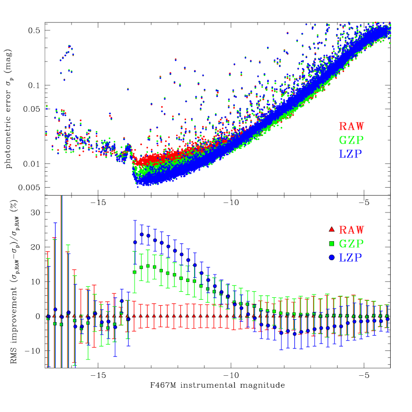
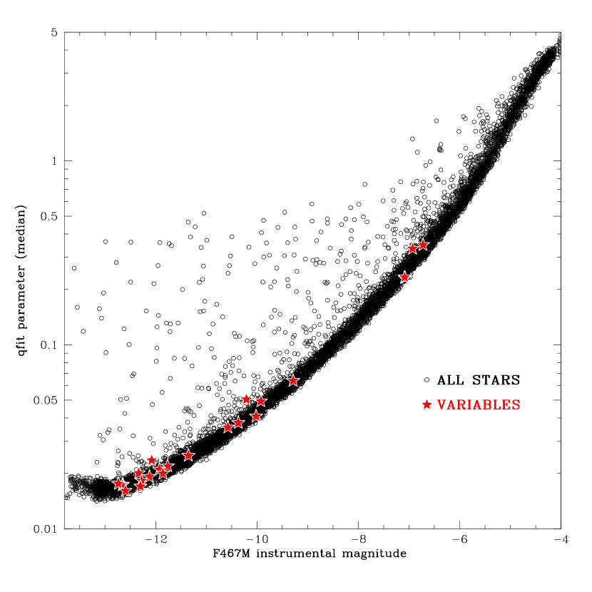
Figure 1: Left, upper panel: Photometric error $\sigma_{p}$ as a function of instrumental magnitude F467M, measured on all stars with three different correction algorithms: none (“RAW”, red points), global zero-point (“GZP”, green) and local zero-point (“LZP”, blue). Saturation occurs at $\mathrm{F467M}\simeq-13.75$. Left, lower panel: “improvement” as a function of F467M, i.e., the percent reduction of RMS compared to raw light curves, averaged on 0.25-mag bins. Colours are coded as above. Right: median value of the fit quality parameter qfit as a function of F467M, all light curves (black circles). Variable stars found by our study (Table 1) are marked with red stars.

2 Data analysis

The full GO-12911 data set was gathered during 120 HST orbits, arranged in 12 epochs made of 10 HST visits each, where each visit is one orbit. Each orbit is filled with five $392$-$396$ s exposures in the blue filter F467M (except for eleven isolated frames for which the F467M exposure time was set to 366 s), and one additional 20-s exposure through a red F775W filter at the beginning of the orbit. The choice of such unorthodox filters was driven by the astrometric requirements of our project. The intermediate-band F467M yields a more monochromatic-like point spread function (PSF), less prone to colour-dependent systematic errors. For the same reason, the Sloan $i^{\prime}$-like F775W filter was preferred over the more commonly used F814W thanks to its better characterised astrometric solution. Its $\sim$$1000$ $\AA$ cut on the red tail does not imply a significant flux loss, because there the total transmission is very low. The F467M filter also has the advantage of suppressing the contaminating light of PSF halos from red giants.

The first visit occurred on 2012 Oct 9, followed by a 100 d gap and then by eleven other visits regularly spaced at a $\sim$24-day cadence. In this work we will focus on a homogeneous subset of 589 “deep” ($392$-$396$ s) F467M images, in order to take advantage of a denser sampling and smaller flux contamination from giants. Data reduction was carried out by modelling an effective PSF (ePSF; Anderson & King 2000) tailored on each frame. Details about the ePSF approaches can be found in Paper I and references therein. Proper motions were derived by matching our data with ACS astrometry by Sarajedini et al. (2007) (GO-10775, PI: Sarajedini), over a baseline of about six years.

It is worth noting that the codes employed are able to extract acceptable photometry even on stars brighter than saturation by collecting the charge bled along the columns of the detector (Gilliland, 2004; Anderson et al., 2008). This is possible thanks to the excellent capability of WFC3/UVIS to conserve the flux even after the pixel full-well is exceeded (Gilliland, Rajan & Deustua, 2010). Each unsaturated star in each exposure was measured by adding up the flux within its central $5\times 5$ pixels, then dividing by the fraction of the star’s light that should have fallen within the aperture (based on the PSF model and the PSF-fitted position of the stars within its central pixel). The aperture for saturated stars started with this $5\times 5$ aperture, but we also had to include all contiguous pixels that were either saturated or neighboring saturated pixels. The total flux was then the flux of the star through the aperture divided by the fraction of the PSF determined to lie within the aperture. In this way, we were able to determine the photometry of the saturated and unsaturated stars in the same system. Fig. 1 shows that the absolute precision of the saturated stars is not as good as that for the unsaturated stars, since the LZP and GZP are constructed to correspond to the $5\times 5$-pixel aperture, not the variable aperture for saturated stars. Nevertheless, the smoothness of our color-magnitude diagram (CMD; Fig. 3) across the F467M saturation boundary at $-13.75$ indicates that there are no systematic differences between photometry for the saturated and unsaturated stars. The reliability of this approach is shown by the quality of the light curves for the 13 RR Lyrae stars (see Sect. 3.1 for details).

Our initial input list was constructed by requiring the detection for each given source in at least 100 out of 589 frames, in order to get light curves spanning a phase coverage large enough to extract a meaningful period analysis from them. This constraint left us with 9 410 sources, all brighter than instrumental magnitude $\mathrm{F467M}\simeq-4$, corresponding to about 40 detected photoelectrons. On the bright side, the most luminous stars reach $\mathrm{F467M}\simeq-17.5$ (corresponding to $V\simeq 12.5$: Fig. 1, upper left panel). This means that the dynamic range of our data set spans more than 13 magnitudes, enabling us to measure stars which are usually saturated and neglected in most surveys.

Most sources among our detections are single, point-like sources belonging to M 4. A small fraction of the sample, however, is made of galaxies, extended objects, unresolved stellar blends and instrumental artefacts. These can be identified by looking at the qfit parameter, a diagnostic value that is related to the goodness of the ePSF fit (Anderson et al., 2008). As the mean $\langle\texttt{qfit}\rangle$ of a light curve is a monotonically increasing function of magnitude (Fig. 1, right panel), a reliable way to identify badly-measured outliers is to compare it with its median value evaluated over magnitude bins. We anticipate that, after the vetting procedure, all the variable stars discussed here are high-confidence point-like sources.

The observing strategy behind the GO-12911 program was optimised for performing high precision astrometry. In order to model and correct all the distortion terms of the astrometric solution, the images were gathered by setting a large-dither pattern of 50 points and changing the telescope roll angle within each astrometric epoch. Stars fall on completely different physical pixels on most frames. While this is a winning choice for the main goal of program, it poses some issues when trying to extract accurate time-resolved photometry. Even when the PSFs are carefully modelled, this approach amplifies the effect of flat field residual errors, intrapixel and pixel-to-pixel inhomogeneities, and other position-dependent effects. As a consequence, subtle second-order systematics are introduced in our photometry, as is evident by examining the raw light curves which share common trends whose shape and amplitude depend on the sky region analysed. A similar behaviour was also observed on data from the ACS/WFC (Advanced Camera for Surveys, Wide Field Channel) in our previous work on NGC 6397 (Nascimbeni et al., 2012). Our approach to minimise such systematics is based on correcting differential light curves by subtracting a local zero-point (LZP), evaluated individually for each target star and each frame.

2.1 Global differential photometry

Before performing a LZP correction, an intermediate and straightforward step is applying a global zero-point correction (GZP). In what follows, we index the individual frames with variable $i$, the 9 410 target stars with the variable $k$ and the subset of sources chosen as comparison stars with $j$. Individual data points from target/reference light curves will be then identified by $m_{i,k}$ and $m_{i,j}$, respectively. The notation $\langle x\rangle_{y}$ represents the averaging of $x$ over the index $y$. Unless otherwise noted, averaging is done by evaluating the median and setting as the associated scatter $\sigma_{\langle x\rangle}$ the $68.27^{\mathrm{th}}$ percentile of the absolute residuals.

As a first step, we chose a common set of reference sources. These are required to be bright, non-saturated ($-13.75<F467M<-10$), point-like and well-fitted (qfit within 2$\sigma$ from the median qfit of all the stars having similar magnitude; this ensures that extended sources and blends are discarded). We also required that they are detected and measured on a minimum number of frames $N_{\mathrm{min}}=500$ over 589, as a reasonable compromise between completeness and FOV coverage. This left us with 1 485 reference stars. For each of them we computed the median raw magnitude $\langle m_{i,j}\rangle_{i}$ by iteratively clipping outliers at $2\sigma$; then each reference raw light curve $m_{i,j}$ was normalised by subtracting $\langle m_{i,j}\rangle_{i}$ from it. A global “trend” $\tau_{i}$ was calculated for each frame $i$ by taking the 2-$\sigma$ clipped median of all available $m_{i,j}-\langle m_{i,j}\rangle_{i}$. The quantity $\tau_{i}$ is the GZP correction to be applied to each point $m_{i,k}$ belonging to target light curves:

$$m^{\prime}_{i,k}=m_{i,k}-\tau_{i}=m_{i,k}-\langle m_{i,j}-\langle m_{i,j}\rangle_{i}\rangle_{j}\textrm{ .}$$ (1)

The pre-normalisation procedure enables us to estimate $\tau_{i}$ without biases, even if a small subset of reference stars is lacking from a given frame. On the other hand, median statistics, as opposed to arithmetic means and RMS, proved to be robust enough against outliers.

If one plots the photometric scatter $\sigma_{\langle m\rangle}$ and $\sigma_{\langle m^{\prime}\rangle}$ as a function of magnitude (Fig. 1, upper left panel, red vs. green points), it is clear that $\sigma_{\langle m^{\prime}\rangle}<\sigma_{\langle m\rangle}$ especially on bright stars ($-13.5<\mathrm{F467M}<-10$). The average decrease in RMS is up to 15% at $\mathrm{F467M}\simeq-13$ (Fig. 1, lower left panel). GZP-correction is therefore effective when compared to raw photometry. Still, upon visual inspection spatial- and magnitude-dependent systematics are still present on the bright side of our sample and require a more sophisticated correction.

2.2 Local differential photometry

In order to build a set of suitable reference light curves to evaluate a LZP correction, one needs to trim down the list of comparison stars by rejecting variables and badly-behaved sources. First we considered the distribution of GZP-corrected scatter $\sigma_{\langle m^{\prime}\rangle}$ as a function of $\langle m^{\prime}_{i,j}\rangle_{i}$, evaluating its median and scatter over magnitude bins; then each star more than $4\sigma$ off the median $\sigma_{\langle m^{\prime}\rangle}$ was discarded from the reference set. The “loose” $4\sigma$ threshold is justified by the need of not rejecting stars which could share common systematics with respect to other target stars; in that case their inclusion in the reference set would be the only way to correct such systematics.

For each pair of target star $k$ and reference star $j$, we constructed a differential light curve by subtracting their raw magnitudes $m_{i,k}$ and $m_{i,j}$ on each frame $i$ where both stars are detected. Then we considered the distribution of the absolute residuals around $\langle m_{i,k}-m_{i,j}\rangle_{i}$, and define the scatter $\sigma_{jk}$ as the $68.27^{\mathrm{th}}$ percentile of such residuals. The quantity $\sigma_{jk}$ is an empirical estimate of how much the reference star $j$ is a “good” reference for the target $k$. We can then assume the quantities $w_{jk}=1/\sigma^{2}_{jk}$ as initial weights to compute a more accurate ZP correction for a given target $k$.

Since we want the correction to be local, we also multiply the weights by a factor $D_{jk}$ which is dependent on the relative on-sky position $\varrho^{2}_{jk}=(x_{j}-x_{k})^{2}+(y_{j}-y_{k})^{2}$ between the reference star ($x_{j}$, $y_{j}$) and the target star ($x_{k}$, $y_{k}$). To avoid using a reference star too close to the target, which could therefore be blended or contaminated, $D_{jk}$ is forced to zero within $r_{0}$. Outside $r_{0}$, we chose to parametrise $D_{jk}$ as a unitary factor up to a inner radius $r_{\mathrm{in}}$, and then as a smooth function which decreases exponentially from one to zero with a $r_{\mathrm{out}}-r_{\mathrm{in}}$ scale radius (i.e., the factor $D_{jk}$ is $1/\mathrm{e}$ at $r_{\mathrm{out}}$):

$$D_{jk}=\left\{\begin{array}[]{cl}0&\textrm{if }\;\varrho_{jk}<r_{0}\\ 1&\textrm{if }\;r_{0}\leq\varrho_{jk}\leq r_{\mathrm{in}}\\ \exp\left[-\left(\frac{\varrho_{jk}-r_{\mathrm{in}}}{r_{\mathrm{out}}-r_{\mathrm{in}}}\right)^{2}\right]&\textrm{if }\;\varrho_{jk}>r_{\mathrm{in}}\textrm{ .}\\ \end{array}\right.$$ (2)

A similar weight factor $M_{jk}$ is imposed on the magnitude difference $\phi_{jk}=|m_{j}-m_{k}|$, as we expect that systematics due to non-linearity and background estimation are magnitude-dependent. The flux boundaries are $f_{\mathrm{in}}$ and $f_{\mathrm{out}}$, respectively:

$$M_{jk}=\left\{\begin{array}[]{cl}1&\textrm{ if }\;\phi_{jk}\leq f_{\mathrm{in}}\\ \exp\left[-\left(\frac{\phi_{jk}-f_{\mathrm{in}}}{f_{\mathrm{out}}-f_{\mathrm{in}}}\right)^{2}\right]&\textrm{ if }\;\phi_{jk}>f_{\mathrm{in}}\textrm{ .}\\ \end{array}\right.$$ (3)

Summarising, the final weights are given by multiplying the above factors:

$$W_{jk}=\left(1/\sigma^{2}_{jk}\right)\cdot D_{jk}\cdot M_{jk}\textrm{ .}$$ (4)

The LZP correction $\tau^{\prime}_{i}$ is evaluated as for the GZP correction (Eq. 1), but this time using the weighted mean of magnitudes of our set of reference stars instead of an unweighted median, where the weights are assigned as $W_{jk}$. A 3$\sigma$ clip is applied on each image $i$ to improve robustness.

Our approach gives larger weights to reference stars which 1) produce a smaller scatter on the target light curve; 2) are geometrically closer to the target as projected on the sky; 3) have a magnitude similar to that of the target. Of course this approach could be easily generalised by introducing weights based on other external parameters, such as colour or background level, for instance.

The five input parameters $r_{0}$, $r_{\mathrm{in}}$, $r_{\mathrm{out}}$, $f_{\mathrm{in}}$, $f_{\mathrm{out}}$ have to be chosen empirically. After some iterations, we set $r_{0}=20$ pix, $r_{\mathrm{in}}=200$ pix, $r_{\mathrm{out}}=300$ pix, $f_{\mathrm{in}}=1.0$ mag, $f_{\mathrm{out}}=1.75$ mag. The improvement of the LZP correction over the GZP one is shown in the left panel of Fig. 1. In the bright, non-saturated end of our sample ($\mathrm{F467M}\simeq-13$) the RMS is lowered by 10-25% on average when compared to GZP-corrected and raw photometry, respectively. On the faintest targets, GZP performs slightly better than LZP because photon noise dominates and GZP is not forced to discard very bright stars as LZP does. For each target, we chose to apply an optimal correction which outputs the light curve having the lowest scatter among the raw one and the GZP- or LZP-corrected ones. From here on all procedures are carried out on such optimal light curves.

2.3 Variable-searching procedures

A battery of software tools to detect both periodic and non-periodic photometric variability was applied to all $9\,410$ corrected light curves. These tools included period-searching algorithms such as the classical Lomb & Scargle periodogram (LS; Lomb 1976; Scargle 1982) and its generalised version GLS (Zechmeister & Kürster, 2009); the Analysis of Variance periodogram (AoV; Schwarzenberg-Czerny 1989); the Box-fitting Least-Squares periodogram (BLS; Kovács, Zucker & Mazeh 2002). The latter is the most sensitive to eclipse-like event, such as those expected from detached eclipsing binaries and planetary transits. A second class of diagnostics was exploited to search for more general types of variability: the alarm variability statistic as described by Tamuz, Mazeh & Zucker (2005), the overall scatter (based on robust median statistics as defined at the beginning of Sect. 2.1) as a function of magnitude, and the RMS after each of the 12 astrometric epochs has been averaged on a single bin, to catch the effects of long-term variability.

Figure 2: Noise-free window function computed over the temporal baseline of our data set; the injected periods are $P_{\mathrm{inj}}=0.3$ days (upper panel) and $P_{\mathrm{inj}}=4.0$ days (lower panel).

We already mentioned that our data set is not optimised to search for periodic variability. One of the most limiting factors is the non-regular cadence, as each astrometric epoch is separated by 24 days. These temporal gaps introduce many spurious frequencies in the periodograms, making the recovery of the true (astrophysical) period problematic, especially for signals at $P<24$ d where most of the variables are expected to be. We illustrate this by injecting noise-free sinusoids over the 589-images time baseline of our WFC3 data set, and then recovering the signal through a GLS periodogram on the synthetic light curve (Fig. 2). In both cases at $P_{\mathrm{inj}}=0.3$ and 4.0 days, we get a “comb” of periodogram peaks instead of a sharp spike, as it would be expected in an optimal sampling regime. When random noise and systematic errors are accounted for, period recovering gets harder, and the 24-day alias induced by sampling becomes the most significant period. For this reason we split our search over two period ranges: 0.1-20 and 20-200 days, analysing each set independently.

To visually supervise all the individual outputs of the analysis described above on more than 9 000 targets would be much too time-consuming and prone to biases. Instead, we selected a shortlist of candidate variables by running the very same analysis on a set of synthetic light curves, sampled at the same epochs as the real data but after having randomly shuffled the magnitude values. In this way, noise and sampling cadence are preserved, while phase coherence is broken: the resulting “synthetic” analysis represents the expected output when an intrinsic signal is not present. We focused on the distribution of diagnostics such as:

1. the periodogram power for the LS, GLS and AoV algorithm (as defined in the original papers, i.e., $P_{X}$ by Scargle 1982, $p(\omega)$ by Zechmeister & Kürster 2009, and $\Theta$ by Schwarzenberg-Czerny 1989, respectively);

2. the SN and SDE statistics (Kovács, Zucker & Mazeh, 2002) and the signal-to-pink noise ratio (as defined by Pont, Zucker & Queloz 2006 and implemented by Hartman et al. 2008) for the BLS periodogram;

3. the alarm index $\mathcal{A}$ (Tamuz, Mazeh & Zucker, 2005) and the visit-binned and unbinned RMS as a function of magnitude, defined as above.

For each of the above diagnostics, the output distribution from the real data was compared with the results from the synthetic light curves, selecting all targets which fall at least 3-$\sigma$ outside the latter distribution. This gave us a list of 401 candidates which were individually inspected. Most of them turned out to be spurious, due to the target being blended, contaminated, or part of an extended source. Very often false positives came from sources with bad photometry on a single visit due to the star falling on a bad pixel or too close to the detector edges. The latter case was the most frequent cause of false positives detected at periods around the 12- or 24-day alias.

3 Results

After the vetting process, only 38 variables survived. They are listed in Table 1. All of them appear to be isolated, point-like sources, following a visual inspection of the images. This is also confirmed by their qfit diagnostic, which is perfectly consistent with the median qfit of well-measured stars of similar magnitude (Fig. 1, right plot; variables are marked with red stars). Their detected periods are clearly distinct from the typical periods due to aliasing or instrumental effects, such as the 96-min orbital period of HST or the 24-day separation between consecutive visits. For the reasons above, we can identify all those 38 stars as genuine astrophysical variables. In Table 1 we also report the Johnson $V$-band magnitude of each variable (obtained by cross-matching our catalogue with that by Sarajedini et al. 2007) and we identify which stars are matched within a 2-$\sigma$ error ellipse with an X-ray source from the Bassa et al. (2004) catalogue. We stress out that the reported $V$ magnitudes represent the average of the values obtained by Sarajedini et al., not an intensity-weighted average throughout the phase of our light curves.

The membership of our variables with respect to M 4 can be assessed with a very high level of confidence by inspecting the proper motion vector-point diagram (VPD), where stars belonging to the cluster and those in the general field appear extremely well separated (Fig. 3, upper left plot). To our purposes the VPD does not need to be calibrated in physical units (${}^{\prime\prime}/\mathrm{yr}$ proper motion); instead, we simply plot the displacement in pixels measured over the baseline between the WFC3 observations and the first astrometric ACS epoch ($\sim$6 years). We found that nearly all variables are cluster members with the only exceptions being ID# 3407 and 3708. As expected, most variables found at magnitudes fainter than the cluster turnoff turned out to be eclipsing binaries, both of contact (cEB) and detached (dEB) subtypes. On most cases this classification is also supported by their position on the CMD, which is shifted up to $\sim$0.75 mag upwards with respect to single, unblended main sequence stars (Fig. 3). A discussion of individual cases follows.

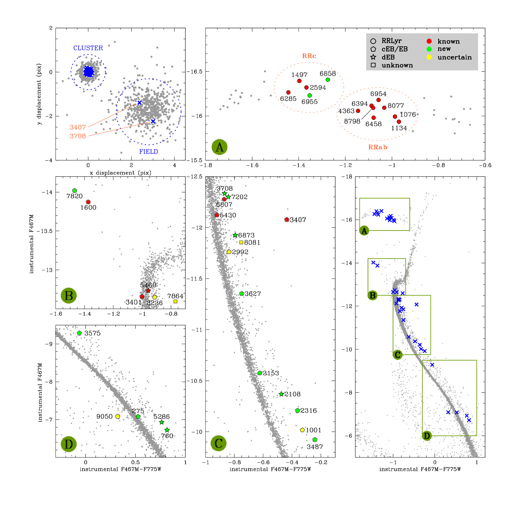
Figure 3: Proper motion vector–point and colour–magnitude diagrams (VPD, CMDs) of M 4 where the detected variables have been highlighted. Upper left: $x$ and $y$ proper motion displacements in physical pixels, for each analysed star (grey dots) and detected variables (blue crosses). Among the latter, only ID#3407 and 3708 appear to not be cluster members. Lower right: instrumental F467M, F775W CMD of M 4 from our data set. Variables are marked with blue crosses. Regions within green boxes ($A$, $B$, $C$, $D$) are zoomed and displayed in the corresponding remaining panels, and labelled according to the legend.

3.1 Notes on individual objects

Known RR Lyrae: ID# 1076, 1134, 1497, 2594, 4363, 6285, 6394, 6458, 6954, 8077, 8798. These are RR Lyr variables known since a long time (Greenstein 1939; re-identified by Shokin & Samus 1996), but whose periods are here determined with much more precision given the 1-yr temporal baseline. The discrimination between RRab (ID# 1076, 1134, 4363, 6394, 6458, 6954, 8077, 8798) and RRc (1497, 2594, 6285) subtypes is obvious. Our classification is confirmed by their position in the CMD (Fig. 3, right panels), with RRab and RRc member being clearly separated by the RR Lyrae gap. The amplitudes of ID# 6285 and 8077 change significantly through the series, due possibly to the Blazhko effect (Kovács, 2009).

New RR Lyrae: ID# 6858, 6955. These are two very close ($1.6^{\prime\prime}$) RR Lyr variables having similar magnitude ($V=13.24$ vs. $13.39$). Such an unusual pair is mostly blended on ground-based images, so it is not surprising that it was classified by Greenstein (1939) as a single RR Lyr with a problematic light curve (C40) and a poorly-constrained period. Other studies recognised it as a visual binary but failed at discovering the true nature of both sources (de Sitter, 1947); therefore C40 has been neglected in many follow-up works on RR Lyrae. We identified both stars as RRc subtypes with periods $P\simeq 0.39$ and $0.29$ d, respectively.

Blue stragglers: ID# 1600 and 7820 are without any doubt cluster members based on their proper motions, and are located in the “blue straggler” region of the CMD. ID# 1600 was already known as a short-period, near equal-mass contact eclipsing binary (Kaluzny, Thompson & Krzeminski, 1997). ID# 7820 also is a contact binary, reported here for the first time. Its periodic modulation at $P\simeq 0.66$ d is detected at high significance. Its primary and secondary minima, showing very unequal depths, suggest a much lower mass ratio than ID# 1600.

Known contact EBs. ID# 3401, 3407, 5430, 6807 are already listed in the Clement et al. (2001) catalogue. They are located close to the turnoff region, with very well defined primary and secondary minima and periods spanning 0.26-0.30 d. Among these, ID# 3407 is the only field star, clearly separated from the cluster in the PM diagram; also it is an X-ray source catalogued as CX13 by Bassa et al. (2004).

Detached EBs: ID# 760, 2108, 3708, 5286, 5460, 6873, 7202 are detached eclipsing binaries, all identified as cluster members by PMs with the only exception of ID# 3708. Among them only ID# 5460 was previously published (as K66, by Kaluzny et al. 2013b). All of them lie in the upper part of the binary main sequence, i.e., are systems with high mass ratios ($q\approx 1$). For that reason their phased light curves are expected to show two eclipses of similar depth between phases 0 and 1. But the period-search algorithms does not know this and therefore might find periods of half the true duration with light curves showing only one eclipse between phases 0 and 1. In some cases, such as for ID# 2108, we have no way of knowing the true period with the current data because of holes in the phased light curves where an eclipse might be happening. In other cases, such as for ID# 5286, the phase coverage seems sufficient to rule out the presence of a second eclipse at the period found, which suggests that the true period is twice as long. Based on such considerations, we give the most likely true periods in Table 1. ID# 2108 also is an X-ray source (CX 28; Bassa et al. 2004), but its light curve shows no sign of stellar activity or interaction. We set the period of ID# 3708 as a lower limit ($P>6.47$ d) since only one eclipse is detectable in our series.

New contact and generic EBs: ID# 2316, 3153, 3487, 3575. The light curves of ID# 2316 and 3153 show an anomalous amount of scatter despite being isolated and well-measured (low qfit); this could be ascribed to starspot-induced variability by one or both components of the eclipsing binary. ID# 3487 is a much fainter EB in the lower MS, observed at low S/N but with recognisable minima and maxima.

Probable EBs: ID# 1001, 2992, 3236, 3627. ID# 1001 shows a sharp $\sim$0.1-mag eclipse overimposed on a pseudo-sinusoidal modulation. If the modulation is interpreted as caused by a “hot spot” or persistent active region then the eclipse appears to be out of phase by about 0.25 (assuming circular orbits, and spin-orbit alignment). No secondary minimum is detected. Light curves of ID# 2992, 3236, 3627 share similar amplitudes (0.05-0.1 mag) and an excess of photometric scatter, but their position in the CMD makes a cEB/dEB classification plausible. ID# 3236 (=CX3) and 3627 (=CX20) are also matched to X-ray sources.

Unclassified/uncertain: ID# 275, 7864, 8081, 9050. The light curve of ID# 275 is clearly periodic with a “double-wave” shape and minima of similar depths. Anyway, its period $P\simeq 0.18$ d is smaller than the usual $\sim$0.22 d cut-off found for MS+MS eclipsing binaries (Norton et al., 2011) and its position on the CMD is very close to the MS ridge, disproving the presence of companions with high $q$. On the other hand, ID# 275 could be a new member of the recently discovered class of ultra-short period M dwarf binaries, first introduced by Nefs et al. (2012). ID# 7864 is a known variable and X-ray source (K52; CX8), and is much brighter than the upper binary sequence envelope, revealing itself as an interacting and/or higher-multiplicity system. This is confirmed by its light curve, showing a strong $P\simeq 0.77$ d periodicity but also a heavily disturbed signal, as already noticed by Kaluzny et al. (2013b). A similar light curve is detected at $P\simeq 0.97$ d on the previously uncatalogued ID# 8081, also a X-ray source (CX11). ID# 9050 is even more peculiar: just as ID # 275, the signal is a clean “double-wave” at $P\simeq 0.18$ d, again an unusually short period for a cEB, but furthermore its position on the CMD is slightly bluer than the MS, suggesting a possible binarity with a bright WD. Only a targeted follow-up could reveal more about the nature of this target.

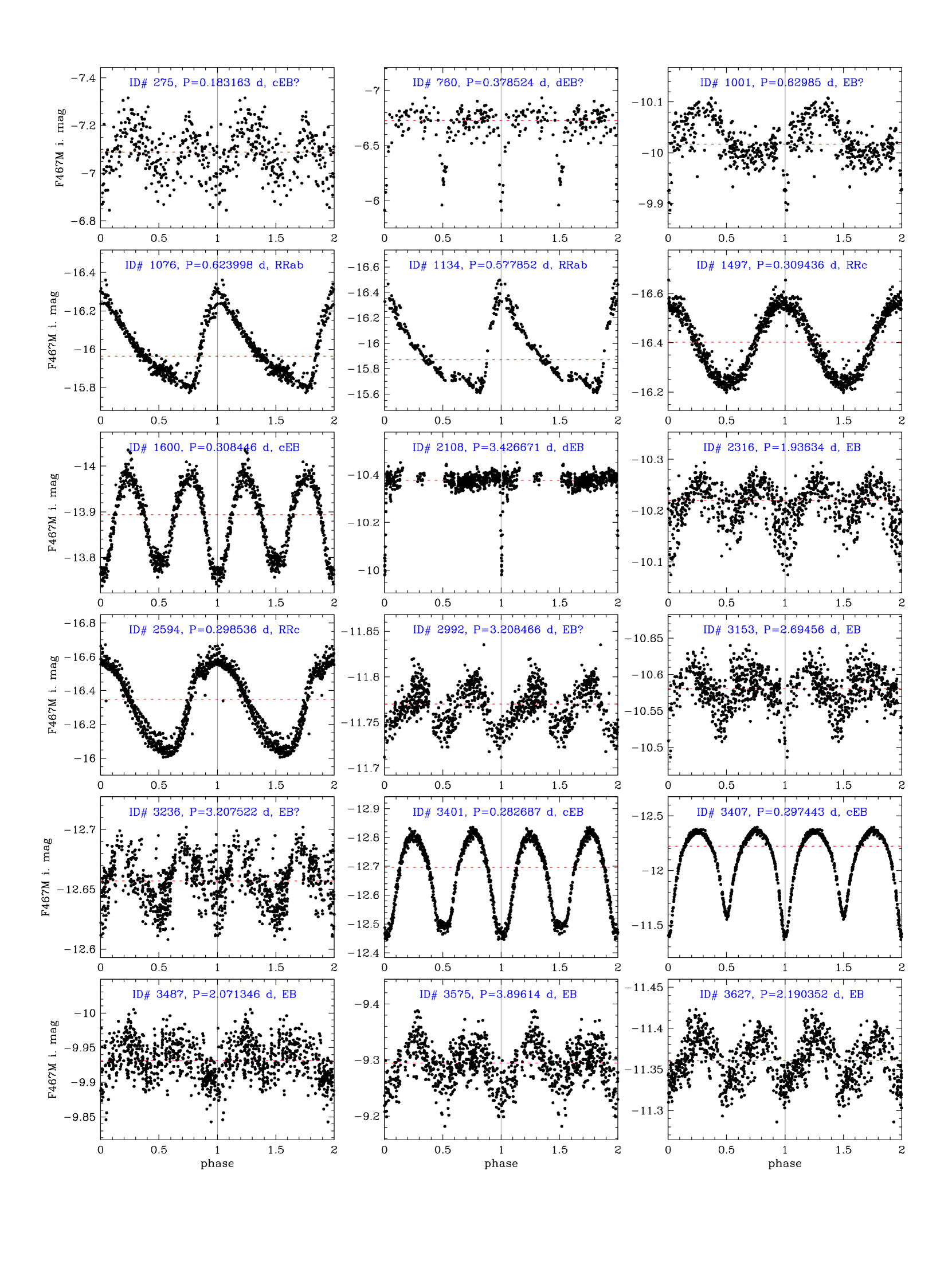
Figure 4: Light curves of variables detected on our data set, folded on the most significant period found by periodograms (figure 1 of 2). Data points are repeated twice over phase for clarity. Target are sorted by ID# code. See Table 1 for coordinates and cross-referencing.

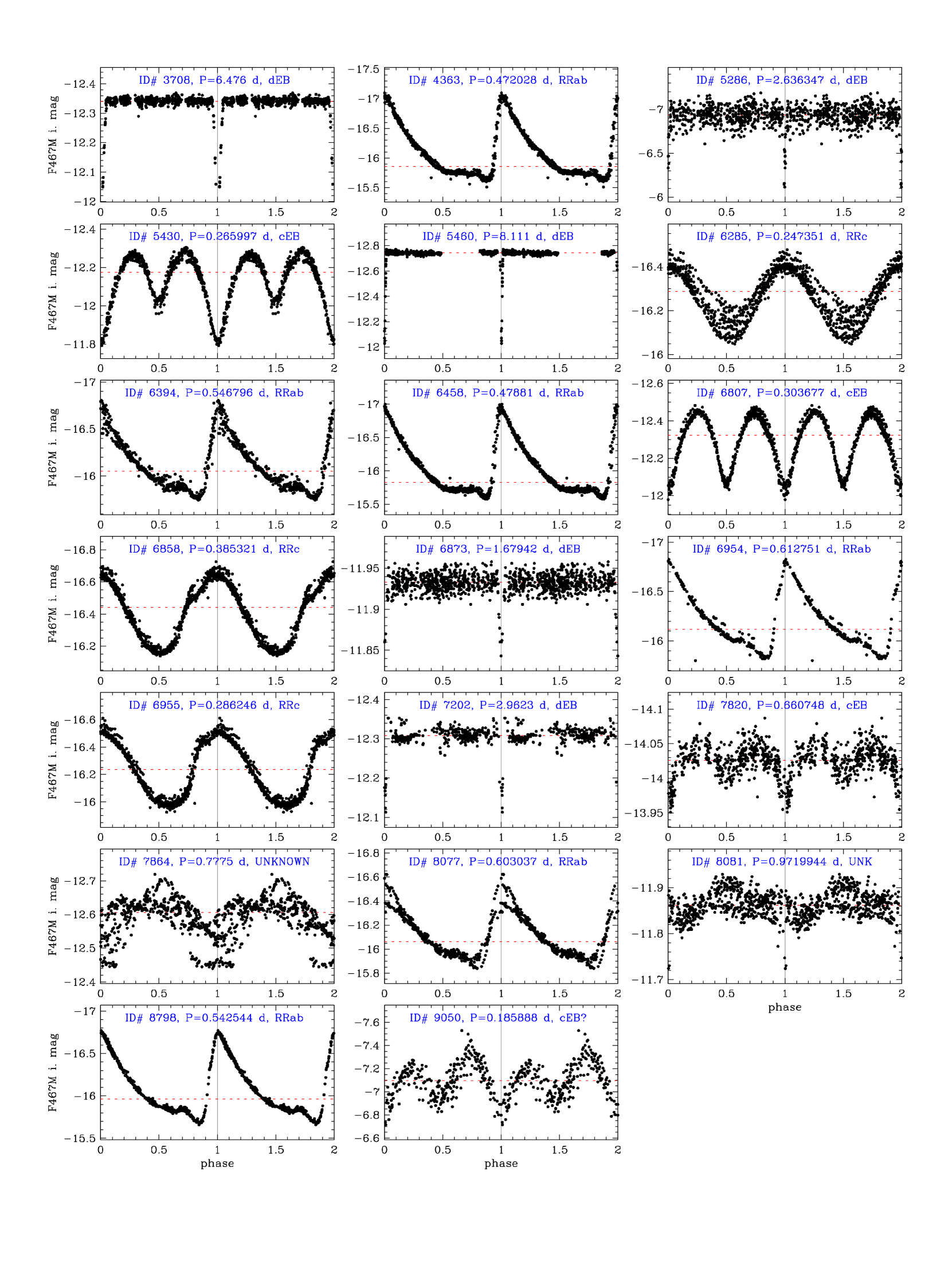
Figure 5: Light curves of variables detected on our data set, folded on the most significant period found by periodograms (figure 2 of 2). Data points are repeated twice over phase for clarity. Target are sorted by ID# code. See Table 1 for coordinates and cross-referencing.

Table 1: Variables found and their characteristics.

$N$	ID#	$\alpha$ (J2000)	$\delta$ (J2000)	F467M	$V$	M	Type	$P$ (days)	X-ref	Notes
1	275	245.90461	$-$26.55051	$-$7.08	21.77	Y	cEB	0.183163	–	MS
2	760	245.88814	$-$26.55350	$-$6.65	22.03	Y	dEB	0.378524	–	BSEQ
3	1001	245.92283	$-$26.53479	$-$10.02	19.30	Y	EB?	0.62985	–	BSEQ
4	1076	245.89437	$-$26.54783	$-$16.00	13.56	Y	RRab	0.623998	C39	HB
5	1134	245.88684	$-$26.55099	$-$15.94	13.91	Y	RRab	0.577852	C38	HB
6	1497	245.89738	$-$26.54333	$-$16.40	13.30	Y	RRc	0.309436	C20	HB
7	1600	245.91036	$-$26.53634	$-$13.88	15.74	Y	cEB	0.308446	C72=K53	BSS
8	2108	245.89580	$-$26.54005	$-$10.36	18.96	Y	dEB	$6.853342^{\ddagger?}$	–	BSEQ; CX28
9	2316	245.88963	$-$26.54161	$-$10.21	19.17	Y	EB	1.93634	–	BSEQ; CX25
10	2594	245.90545	$-$26.53228	$-$16.32	13.05	Y	RRc	0.298536	C23	HB
11	2992	245.89616	$-$26.53445	$-$11.76	17.64	Y	EB?	3.208466	–	MS/BSEQ
12	3153	245.89446	$-$26.53451	$-$10.57	18.91	Y	EB	2.69456	–	MS/BSEQ; CX21
13	3236	245.90870	$-$26.52718	$-$12.65	16.89	Y	EB?	3.207522	–	BSEQ/TO; CX3
14	3401	245.90329	$-$26.52891	$-$12.66	16.79	Y	cEB	0.282687	C67=K48	TO; CX15
15	3407	245.89302	$-$26.53385	$-$12.08	16.98	N	cEB	0.297443	C68=K49	NM; CX13
16	3487	245.90270	$-$26.52871	$-$9.93	19.30	Y	EB	2.071346	–	BSEQ
17	3575	245.91544	$-$26.52222	$-$9.29	19.85	Y	EB	3.89614	–	BSEQ
18	3627	245.90375	$-$26.52755	$-$11.36	18.09	Y	EB	2.190352	–	MS/BSEQ; CX20
19	3708	245.90634	$-$26.52592	$-$12.33	17.17	N	dEB	$>$6.476	–	NM; one eclipse
20	4363	245.89960	$-$26.52604	$-$15.97	13.70	Y	RRab	0.472028	C21	HB
21	5286	245.89808	$-$26.52231	$-$6.92	21.87	Y	dEB	$5.272694^{\ddagger}$	–	BSEQ
22	5430	245.88048	$-$26.53014	$-$12.13	17.53	Y	cEB	0.265997	C69=K50	MS
23	5460	245.88432	$-$26.52812	$-$12.73	16.80	Y	dEB	8.111	K66	TO
24	6285	245.88155	$-$26.52519	$-$16.27	13.60	Y	RRc	0.247351	C37	HB
25	6394	245.90840	$-$26.51161	$-$16.12	13.36	Y	RRab	0.546796	C24	HB
26	6458	245.89448	$-$26.51795	$-$15.92	13.72	Y	RRab	0.47881	C18	HB
27	6807	245.88831	$-$26.51917	$-$12.28	17.08	Y	cEB	0.303677	C70=K51	BSEQ
28	6858	245.90195	$-$26.51230	$-$16.41	13.24	Y	RRc	0.385321	C40$\dagger$	HB
29	6873	245.89321	$-$26.51636	$-$11.93	17.56	Y	dEB	$3.358846^{\ddagger}$	–	BSEQ
30	6954	245.91415	$-$26.50592	$-$16.18	13.07	Y	RRab	0.612751	C25	HB
31	6955	245.90169	$-$26.51190	$-$16.23	13.39	Y	RRc	0.286246	C40$\dagger$	HB
32	7202	245.86887	$-$26.52611	$-$12.30	17.20	Y	dEB	$5.925962^{\ddagger?}$	–	BSEQ
33	7820	245.90261	$-$26.50605	$-$14.02	15.76	Y	cEB	0.660748	–	BSS
34	7864	245.88111	$-$26.51606	$-$12.58	16.92	Y	UNK	—	C71=K52	above BSEQ; CX8
35	8077	245.90387	$-$26.50362	$-$16.09	13.17	Y	RRab	0.603037	C22	HB
36	8081	245.88501	$-$26.51263	$-$11.86	17.65	Y	UNK	0.971994	–	BSEQ; CX11
37	8798	245.88532	$-$26.50639	$-$16.09	13.55	Y	RRab	0.542544	C16	HB
38	9050	245.89351	$-$26.49984	$-$7.09	21.95	Y	cEB?	0.185888	–	under the MS

Notes. The columns give: a progressive number $N$, the ID code of the source according to our catalogue, the equatorial coordinates $\alpha$ and $\delta$ at epoch 2000.0, the instrumental magnitude in F467M and the standard Johnson $V$ magnitude from Sarajedini et al. (2007), a membership flag derived from the VPD, the variability class assigned by our study, the most probable photometric period $P$ (where detectable), the cross-references to the variable catalogues by Kaluzny et al. (2013b) (letter K) and Clement et al. (2001) (letter C), and some notes. Notes are codified as follows: MS = main sequence star, BSEQ = binary sequence star (between fiducial MS and MS+0.75 mag), HB = horizontal branch, BSS = blue straggler star, CX = X-ray source from the catalogue by Bassa et al. (2004), TO = turn-off star, NM = not a cluster member. A few periods of dEBs, marked with a $\ddagger$, have been doubled with respect to the best-fit periodogram solution, following astrophysical arguments (see Sec. 3.1 for details); two cases are ambiguous, and marked with an additional question mark. The two variables marked by $\dagger$ in the X-ref field were once classified as a single, atypical RR Lyr (Clement et al. 2001 and references therein).

Table 2: Light curves of the variables found.

ID#	BJD(TDB)	F467M	$\Delta$F467M	$x$	$y$	qfit
1001	2456209.701194	-10.0180	0.0168	2653.966	2571.443	0.037
1001	2456209.740334	-10.0160	0.0168	2653.973	2571.472	0.046
1001	2456209.746422	-10.0060	0.0168	2653.999	2571.477	0.032
1001	2456209.752509	-10.0130	0.0168	2653.973	2571.466	0.039
1001	2456209.764684	-9.9920	0.0168	2653.994	2571.487	0.031
1001	2456209.806845	-10.0040	0.0168	2654.001	2571.439	0.033
1001	2456209.812933	-10.0110	0.0168	2653.990	2571.455	0.037
1001	2456209.819020	-10.0080	0.0168	2653.991	2571.449	0.039
1001	2456209.825108	-10.0200	0.0168	2653.965	2571.461	0.037
1001	2456209.831195	-10.0035	0.0168	2653.963	2571.475	0.048

Notes. Table 2 is published in its entirety as a machine-readable table in the online version of this article and the Centre de Donees Strasbourg (CDS). A portion is shown here for guidance regarding its form and content. The columns give: the ID code of the source according to our catalogue (see Table 1), the mid-exposure time in the BJD-TDB time standard (Eastman, Siverd & Gaudi, 2010), the instrumental magnitude in F467M and the associated photometric error, the $x$ and $y$ centroid position on the chip, and the qfit quality parameter.

4 Discussion and Conclusions

In the previous sections we described how we performed a search for photometric variability among a sample of 9410 stars in a field imaged by HST on the core of the globular cluster M 4. Such a search yielded 38 variable stars; all but two are cluster members, and 20 are reported here for the first time. Quite surprisingly, two newly (re-)classified sources are a pair of bright but blended RR Lyrae, whose true nature has been unveiled by the superior angular resolution of space-based imaging. A few candidates cannot be assigned to standard variability classes, being aperiodic, multiperiodic, or lying in unusual regions of the CMD.

We did not detect any signal which could be interpreted as a transit by planet-sized objects orbiting around solar-type stars (i.e., box-shaped eclipses having photometric depth smaller than 0.03 mag). Many intrinsic factors in our data set are strongly limiting a transit search, above all sparse temporal sampling (which decreases phase coverage, and worsens the effects of long-term stellar variability) and large-scale dithering (which boosts position-dependent systematic errors). As only planets among the relatively rare “hot Jupiter” class are within reach of such a search, the statistical significance of our null detection is probably very low. We will investigate this further in a forthcoming paper of the “M 4 core project” series focused on transit search, which will also analyse time-series photometry from the parallel ACS fields.

The overall completeness level of our search is difficult to quantify without posing very special assumptions about the shape and period of the photometric signal to be recovered. However, we note that we firmly detected variables having photometric amplitudes on the order of a few hundredths of magnitude even in the fainter half of our sample (such as ID# 1001, 3487, 3575, 5286). Even though periodograms are aliased at some characteristic frequencies by the particular sampling cadence of our data (Fig. 2), phase coverage is complete up to periods of about six days. Merging the picture, this means that eclipsing contact binaries should be detectable with a completeness factor close to one, with only rare exceptions expected from very grazing systems, or from binaries with mass ratios $q$ much smaller than one.

About half of the reported variables (21, of which 19 are high-confidence cluster members) are certain or probable eclipsing binaries. As we detected 19 EBs among 5 488 MS stars with $-12.75<\textrm{F467M}<-7.0$, or –restricting the magnitude range to brighter targets– 16 EBs among 4 080 MS stars with $-12.75<\mathrm{F467M}<-9.0$, we estimate an observed EBs fraction of about 0.3-0.4%. This value is approximately consistent with the measured photometric binary fraction in the core of $14.8\%\pm 1.4\%$ (Milone et al. 2012), when allowance is made for the low fraction of binaries which are expected to exhibit eclipses. Using population synthesis, Söderhjelm & Dischler (2005) show that the fraction of all F and G stars exhibiting eclipses with a depth of a few tenths of a magnitude and a period of a day is about 3%. The population they studied had a binary fraction of 80%, however, and so the corresponding result for the core of M 4 would be expected to be about 0.5%, i.e., close to our results. A more precise discussion depends on several factors, such as the details of the period distribution of the observed binaries, dynamical erosion of the binary population, and the initial binary distributions assumed in the population synthesis. Indeed the observations reported in this paper are likely to be a useful constraint on our future dynamical modelling of M 4.

As a final remark, we note that the dEBs that are cluster members can potentially be used for obtaining precise cluster parameters, insights into multiple-populations of the cluster and stellar evolution tests in general (paper I, Brogaard et al. 2012, Milone et al. 2014). This requires however that the dEBs are bright enough for spectroscopic measurements. Based on our experience from dEBs in the open cluster NGC6791, four of the dEBs we identify in M 4 (ID# 5460, 7202, 6873, and 2108) are within reach of current spectroscopic facilities such as UVES at the Very Large Telescope. Adding also the additional dEBs found and analysed by Kaluzny et al. (2013a) makes a sample of six dEBs in the turn-off and upper MS of M 4 with great potential for improved cluster insights. The two low-mass dEB systems found on the lower main sequence ($V\simeq 22$; ID# 760 and 5286) are too faint for current spectroscopic facilities, but interesting potential targets for a future ELT. We note that M 4 will be in one of the fields of the K2 mission (Howell et al., 2014), and that observing these six dEBs with K2 would solve period ambiguities and provide full-coverage light curves valuable for their analysis.

References

- Anderson & King (2000) Anderson J., King I. R., 2000, PASP, 112, 1360
- Anderson et al. (2008) Anderson J. et al., 2008, AJ, 135, 2055
- Bassa et al. (2004) Bassa C. et al., 2004, ApJ, 609, 755
- Bedin et al. (2013) Bedin L. R. et al., 2013, Astronomische Nachrichten, 334, 1062
- Bedin et al. (2009) Bedin L. R., Salaris M., Piotto G., Anderson J., King I. R., Cassisi S., 2009, ApJ, 697, 965
- Brogaard et al. (2012) Brogaard K. et al., 2012, A&A, 543, A106
- Clement et al. (2001) Clement C. M. et al., 2001, AJ, 122, 2587
- de Sitter (1947) de Sitter A., 1947, Bull. Astron. Inst. Netherlands, 10, 287
- Eastman, Siverd & Gaudi (2010) Eastman J., Siverd R., Gaudi B. S., 2010, PASP, 122, 935
- Ferdman et al. (2004) Ferdman R. D. et al., 2004, AJ, 127, 380
- Gilliland (2004) Gilliland R. L., 2004, ACS CCD Gains, Full Well Depths, and Linearity up to and Beyond Saturation. Tech. rep.
- Gilliland, Rajan & Deustua (2010) Gilliland R. L., Rajan A., Deustua S., 2010, WFC3 UVIS Full Well Depths, and Linearity Near and Beyond Saturation. Tech. rep.
- Greenstein (1939) Greenstein J. L., 1939, ApJ, 90, 387
- Harris (1996) Harris W. E., 1996, AJ, 112, 1487
- Hartman et al. (2008) Hartman J. D., Gaudi B. S., Holman M. J., McLeod B. A., Stanek K. Z., Barranco J. A., Pinsonneault M. H., Kalirai J. S., 2008, ApJ, 675, 1254
- Heggie & Hut (2003) Heggie D., Hut P., 2003, The Gravitational Million-Body Problem: A Multidisciplinary Approach to Star Cluster Dynamics
- Howell et al. (2014) Howell S. B. et al., 2014, ArXiv e-prints
- Kaluzny et al. (2012) Kaluzny J., Rozanska A., Rozyczka M., Krzeminski W., Thompson I. B., 2012, ApJ, 750, L3
- Kaluzny, Thompson & Krzeminski (1997) Kaluzny J., Thompson I. B., Krzeminski W., 1997, AJ, 113, 2219
- Kaluzny et al. (2013a) Kaluzny J. et al., 2013a, AJ, 145, 43
- Kaluzny et al. (2013b) Kaluzny J., Thompson I. B., Rozyczka M., Krzeminski W., 2013b, Acta Astron., 63, 181
- Kovács (2009) Kovács G., 2009, in American Institute of Physics Conference Series, Vol. 1170, American Institute of Physics Conference Series, Guzik J. A., Bradley P. A., eds., pp. 261–272
- Kovács, Zucker & Mazeh (2002) Kovács G., Zucker S., Mazeh T., 2002, A&A, 391, 369
- Leavitt & Pickering (1904) Leavitt H. S., Pickering E. C., 1904, Harvard College Observatory Circular, 90, 1
- Lomb (1976) Lomb N. R., 1976, Ap&SS, 39, 447
- Milone et al. (2014) Milone A. P. et al., 2014, MNRAS, 439, 1588
- Milone et al. (2012) Milone A. P. et al., 2012, A&A, 540, A16
- Nascimbeni et al. (2012) Nascimbeni V., Bedin L. R., Piotto G., De Marchi F., Rich R. M., 2012, A&A, 541, A144
- Nefs et al. (2012) Nefs S. V. et al., 2012, MNRAS, 425, 950
- Norton et al. (2011) Norton A. J. et al., 2011, A&A, 528, A90
- Pont, Zucker & Queloz (2006) Pont F., Zucker S., Queloz D., 2006, MNRAS, 373, 231
- Sarajedini et al. (2007) Sarajedini A. et al., 2007, AJ, 133, 1658
- Sawyer (1931) Sawyer H. B., 1931, Harvard College Observatory Circular, 366, 1
- Scargle (1982) Scargle J. D., 1982, ApJ, 263, 835
- Schwarzenberg-Czerny (1989) Schwarzenberg-Czerny A., 1989, MNRAS, 241, 153
- Shokin & Samus (1996) Shokin Y. A., Samus N. N., 1996, Astronomy Letters, 22, 761
- Sigurdsson et al. (2003) Sigurdsson S., Richer H. B., Hansen B. M., Stairs I. H., Thorsett S. E., 2003, Science, 301, 193
- Söderhjelm & Dischler (2005) Söderhjelm S., Dischler J., 2005, A&A, 442, 1003
- Tamuz, Mazeh & Zucker (2005) Tamuz O., Mazeh T., Zucker S., 2005, MNRAS, 356, 1466
- Trager, King & Djorgovski (1995) Trager S. C., King I. R., Djorgovski S., 1995, AJ, 109, 218
- Zechmeister & Kürster (2009) Zechmeister M., Kürster M., 2009, A&A, 496, 577