Bistable protein distributions in rod-shaped bacteria

Abstract

The distributions of many proteins in rod-shaped bacteria are far from homogenous. Often they accumulate at the cell poles or in the cell center. At the same time, the copy number of proteins in a single cell is relatively small making the patterns noisy. To explore limits to protein patterns due to molecular noise, we studied a generic mechanism for spontaneous polar protein assemblies in rod-shaped bacteria, which is based on cooperative binding of proteins to the cytoplasmic membrane. For mono-polar assemblies, we find that the switching time between the two poles increases exponentially with the cell length and with the protein number.

I Introduction

Though usually small in size, bacteria display a remarkable degree of spatial order Shapiro:2009bj ; kruse12 . In the simplest case, proteins are in a controlled way unevenly distributed between the two halves of rod-shaped bacteria like Escherichia coli or Bacillus subtilis. Examples for asymmetric distributions are provided by the accumulation of chemotactic receptors at the poles of E. coli Maddock:1993tu , the localisation of Spo0J/Soj proteins close to the poles of B. subtilis Quisel:1999uh ; Marston:1999uj , or the Min proteins in E. coli, which periodically switch between the two cell halves Raskin:1999vr . More refined structures are the Z-ring that localises at the site of cell division Bi:1991fr , the localisation as a string of pearls of magnetosomes involved in bacterial magnetotaxis Bazylinski:2004jx , and the distribution of flagella of various motile bacteria Chevance:2008bq .

Typically, the spatial distribution of proteins is linked to their function. Tom Duke was among the first to realise the importance of spatial structures for signalling. In the context of bacterial chemotaxis, he argued that the formation of receptor complexes increases sensitivity Duke:1999td . Another example is provided by the Min-protein oscillations that are used to select the site of cell division Loose:2011dd . To give just one more example, the linear arrangement of magnetosomes produces a strong enough magnetic dipole moment for bacteria to orient along the field lines of the geomagnetic field Bazylinski:2004jx .

As a consequence of their functional importance, these spatial structures need to be maintained for a proper working of the cell. However, usually, the relatively small copy number of proteins in a cell, which typically ranges between less than ten to a few thousands, implies that molecular noise may severely restrict their life-time. In some cases, noise does not seem to be a problem. For example, the Spo0J/Soj proteins stochastically switch between the two nucleoids without impairing the fitness of B. subtilis Quisel:1999uh ; Marston:1999uj . In other cases, molecular mechanisms assure the stability of protein patterns. For instance, numerical analysis of the Min-protein dynamics has revealed that the oscillatory pattern is robust against molecular noise Kerr:2006bh ; Fange:2006ii ; Arjunan:2010fd . So, we face the question of how noise affects spatial protein distributions.

The influence of molecular noise on bacterial processes has intensively been studied during recent years Eldar:2010kk . In this context, a particular focus has been put on bistable systems Balazsi:2011bw . Spatially extended systems have received less attention, though. One example is provided by the Spo0J/Soj system mentioned above Quisel:1999uh ; Marston:1999uj ; Doubrovinski:2005cm . Also the Min proteins in E. coli were studied in this context and found to stochastically switch between the two cell halves in sufficiently small cells after moderate over-expression FischerFriedrich:2010hv ; Sliusarenko:2011cz ; Bonny:2013gt .

The spatial structures mentioned above have in common that the proteins in question assemble on a support, for example, the membrane or the nucleoid. Consequently, spatial cues on these scaffolds might underlie the formation of the protein aggregates. In an extreme case, the proteins would not interact with each other but rather move in a potential landscape imposed by the spatial cues on the scaffold. An alternative is protein self-organisation kruse12 . Mechanisms for self-organisation have been proposed for Spo0J/Soj Doubrovinski:2005cm and the Min proteins Howard:2005dd . For the latter, the possibility of self-organisation has been demonstrated in reconstitution experiments Loose:2008ca ; Zieske:2013fi .

In this work, we study the switching between two self-organised states of a spatially extended system in the weak-noise limit. In this case, typically, one cannot use Kramers rate theory, which relies on the existence of a potential. Instead, a generalisation of Kramers’ theory based on a pseudo-potential method can be employed BENJACOB:1982vo ; KUPFERMAN:1992wy ; Maier:1993vv . In a biological context, this method has been applied to bistable genetic switches Roma:2005jj ; Assaf:2011iw and to bidirectional transport of molecular motors Guerin:2011ed ; Guerin:2011bk . Our study is motivated by the heterogenous protein distributions in rod-shaped bacteria described above. Heterogeneity of the distributions results from cooperative protein attachment to the membrane, which is motivated by studies of the Spo0J/Soj dynamics Doubrovinski:2005cm and the Min system Huang:2003bc . The molecular origin of cooperative binding remains to be understood, but has been very successful in these contexts. After defining the model, we will first perform stochastic simulations. To get further insight, we will perform a mean-field analysis and then follow the approach in Hildebrand:1996ck to establish the corresponding Fokker-Planck equation for the dominant modes. Employing a WKB ansatz, we will solve the Fokker-Planck equation and obtain the switching time as in Ref. Maier:1993vv . The work concludes with some remarks about possible generalisations.

II Stochastic dynamics for molecules forming membrane clusters

II.1 The Chemical Master Equation

In the following, we consider the following processes: 1) Cytoplasmic molecules can bind to the membrane, with binding being favoured in regions, where membrane-bound molecules are already present; 2) spontaneous detachment of membrane-bound molecules; 3) diffusion of cytoplasmic and membrane-bound molecules, see Fig. 1. We will consider the dynamics in rod-like bacteria like E. coli and approximate the shape by a cylinder of length $L$ and radius $R$, where we assume the top and the bottom to be unavailable for binding. Furthermore, we will restrict attention to situations where the protein distribution is invariant with respect to rotations around the cylinder axis. Possible consequences of these assumptions are discussed below. In direction of the long axis, the membrane is decomposed into compartments of length $\ell$. We will assume that particles within a compartment are well-mixed. This implies that we consider processes on time-scales that are larger or on the order of $\ell^{2}/D_{\mathrm{m}}$, where $D_{\mathrm{m}}$ is the diffusion constant of membrane-bound molecules. For cytoplasmic molecules, we assume a compartment that extends from the membrane to the cell center and again, we will consider it to be well-mixed. This implies that we are restricted to time-scales larger or of the order of $\tau\approx R^{2}/D_{\mathrm{c}}$, where $D_{\mathrm{c}}$ is the cytosolic diffusion constant. For $R\approx 0.5\mu\mathrm{m}$ and $D_{\mathrm{c}}\approx 15\mu\mathrm{m}^{2}/\mathrm{s}$ we get $\tau\approx 20\mathrm{ms}$.

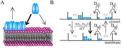
Figure 1: Illustration of the system dynamics and geometry. A) Illustration of the molecular processes considered in this work. They comprise spontaneous and cooperative attachment to as well as spontaneous detachment from the membrane. B) Schematic of the geometry considered. The system consists of two linear arrays of bins of length $\ell$ that are assumed to be well mixed. The two arrays, respectively, represent the cytoplasm and the membrane. The rates for the different processes are indicated.

The rate of spontaneous attachment to the membrane is denoted by $\omega_{\mathrm{a}}$, whereas the rate of spontaneous detachment is $\omega_{\mathrm{d}}$. The rate of co-operative membrane-binding in compartment $i$ is given by $\omega_{\mathrm{c}}n_{\mathrm{m},i}(n_{\mathrm{m},i}-1)/(\Omega^{2}\ell^{2})$. In this expression, $n_{\mathrm{m},i}$ is the number of membrane-bound molecules in compartment $i$ – the corresponding number of cytosolic molecules will be denoted by $n_{\mathrm{c},i}$ – and $\Omega$ is the total number of molecules in the system. We make the scaling of the co-operative binding term with the compartment size and the total molecule number explicit, because we will later consider the limit of large molecule numbers $\Omega\to\infty$ and the continuum limit $\ell\to 0$.

The corresponding Chemical Master Equation for the evolution of the joint probability $P(\{n_{\mathrm{c},i}\}_{i=1,\ldots,N},\{n_{\mathrm{m},i}\}_{i=1,\ldots,N};t)$ can be written as

$$\frac{dP}{dt} =\sum_{i}\omega_{\mathrm{a}}\big{(}\mathbb{E}_{\mathrm{c},i}^{+}\mathbb{E}_{\mathrm{m},i}^{-}-1\big{)}n_{\mathrm{c},i}P+\sum_{i}\frac{\omega_{\mathrm{c}}}{\Omega^{2}\ell^{2}}\big{(}\mathbb{E}_{\mathrm{c},i}^{+}\mathbb{E}_{\mathrm{m},i}^{-}-1\big{)}n_{\mathrm{c},i}n_{\mathrm{m},i}(n_{\mathrm{m},i}-1)P+\sum_{i}\omega_{\mathrm{d}}\big{(}\mathbb{E}_{\mathrm{c},i}^{-}\mathbb{E}_{\mathrm{m},i}^{+}-1\big{)}n_{\mathrm{m},i}P$$

$$+\sum_{i}\frac{D_{\mathrm{c}}}{\ell^{2}}\mathbb{E}_{\mathrm{c},i}^{-}\mathbb{E}_{\mathrm{c},i+1}^{+}n_{\mathrm{c},i+1}P+\sum_{i}\frac{D_{\mathrm{c}}}{\ell^{2}}\mathbb{E}_{\mathrm{c},i}^{-}\mathbb{E}_{\mathrm{c},i-1}^{+}n_{\mathrm{c},i-1}P-2\sum_{i}\frac{D_{\mathrm{c}}}{\ell^{2}}n_{\mathrm{c},i}P$$

$$+\sum_{i}\frac{D_{\mathrm{m}}}{\ell^{2}}\mathbb{E}_{\mathrm{m},i}^{-}\mathbb{E}_{\mathrm{m},i+1}^{+}n_{\mathrm{m},i+1}P+\sum_{i}\frac{D_{\mathrm{m}}}{\ell^{2}}\mathbb{E}_{\mathrm{m},i}^{-}\mathbb{E}_{\mathrm{m},i-1}^{+}n_{\mathrm{m},i+1}P-2\sum_{i}\frac{D_{\mathrm{m}}}{\ell^{2}}n_{\mathrm{m},i}P$$ (1)

In this expression $\mathbb{E}_{\mathrm{c},i}^{\pm}$ denote the particle creation and annihilation operators in compartment $i$ such that, for example, $\mathbb{E}_{\mathrm{c},i}^{+}f(\{n_{\mathrm{c},j}\}_{j=1,\ldots,N},\{n_{\mathrm{m},j}\}_{j=1,\ldots,N})=f(\ldots,n_{\mathrm{c},i}+1,\ldots,\{n_{\mathrm{m},j}\}_{j=1,\ldots,N})$. The corresponding operators for membrane bound compartments are denoted by $\mathbb{E}_{\mathrm{m},i}^{\pm}$. The terms in the first line of the Chemical Master Equation account for attachment to and detachment from the membrane, the next two lines capture diffusion of cytoplasmic and membrane-bound molecules.

II.2 Numerical solution of the chemical Master equation

We numerically analyse the Chemical Master Equation by combining the Gillespie algorithm with the next subvolume method Elf:2004fv . Explicitly, in a given state, we determine for each compartment $j$ the total rate of a change in the number of either the bound or unbound particles. For each compartment, we then draw a random number to determine the time at which the next event occurs and perform the corresponding action for the compartment with the shortest waiting time. We then go back and update the total rates of all compartments and continue as before.

In Figure 2 we present the results of a simulation for a system length of 5.2$\mu$m. The kymograph in Fig. 2A shows that the particles accumulate in the vicinity of one end or “cell pole”. At random times, the particles switch to the opposite pole. The distribution of switching times has a mean value $\langle\tau\rangle=4965$s and is rather broad, see Fig. 2C, with a standard deviation $\sigma_{\tau}=5487$s. The time-averaged profile of particles in one cell half agrees well with the profile obtained from the mean-field equations (15) and (16), see Fig. 2B, which will be introduced and discussed below. It should be noted that, as for all continuum theories, the agreement between the mean-field theory and the stochastic simulations depends on the choice of $\ell$ in the stochastic simulations. Each bin should contain on average a sufficiently large number of molecules such that a continuum approach is appropriate. At the same time $\ell$ should be small compared to spatial features of the protein distribution.

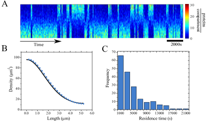
Figure 2: Stochastic dynamics of membrane clustering. A) Colour-coded protein distribution as a function of time. B) Time-averaged profile of proteins residing in one cell half (blue dots) and mean field profile (black line). C) Distribution of residence times. Parameters are $D_{\mathrm{c}}=10\mu$m²s^-1, $D_{\mathrm{c}}=0.1\mu$m²s^-1, $\omega_{\mathrm{a}}=0.1$s^-1, $\omega_{\mathrm{d}}=0.1$s^-1, $\omega_{\mathrm{c}}=1\mu$m²s^-1, $L=5.2\mu$m, $\ell=0.2\mu$m, $\Omega=187$ (A,C), and $\Omega=260$ (B).

III The functional Fokker-Planck equation

In order to go beyond the numerical analysis of the system, we will in this section derive a functional Fokker-Planck Equation from the Chemical Master Equation (1). To this end will perform in a first step an expansion in terms of the inverse molecule number $1/\Omega$, which is a form of van Kampen’s system size expansion. In a second step, we will take the continuum limit $\ell\to 0$. The resulting equation will first be analysed in the deterministic limit $\Omega\to\infty$. Then, we will use a Galerkin ansatz to obtain an equation that is amenable to analysis of the influence of molecular noise on the system behaviour, which will be carried out in the next section.

III.1 System size expansion and continuum limit

Let us consider the case of $\Omega\gg 1$. In each compartment with large occupancies, $n_{\mathrm{c},i}\gg 1$ and $n_{\mathrm{m},i}\gg 1$, we can approximate the creation and annihilation operators of cytosolic and membrane-bound molecules, $\mathbb{E}_{\mathrm{c},i}^{\pm}$ and $\mathbb{E}_{\mathrm{m},i}^{\pm}$, respectively, by

$$\mathbb{E}_{\mathrm{c},i}^{\pm} \approx 1\pm\frac{\partial}{\partial n_{\mathrm{c},i}}+\frac{1}{2}\frac{\partial^{2}}{\partial n_{\mathrm{c},i}^{2}}$$ (2)

$$\mathbb{E}_{\mathrm{m},i}^{\pm} \approx 1\pm\frac{\partial}{\partial n_{\mathrm{m},i}}+\frac{1}{2}\frac{\partial^{2}}{\partial n_{\mathrm{m},i}^{2}}\quad.$$ (3)

Formally, this corresponds to an expansion in the inverse molecule number up to second order. For large but finite values of $\Omega$, the above condition might not be fulfilled for all compartments at all times and higher orders of the approximation should in principle be taken into account. Still, we will see that the ensuing equations give a quantitative account of the system behaviour. In the same spirit, we will also replace from now on the factor $n_{\mathrm{m},i}-1$ in the co-operative binding term by $n_{\mathrm{m},i}$. Explicitly, the Fokker-Planck Equation resulting from the Chemical Master Equation (1) reads

$$\frac{dP}{dt}= -\sum_{i}\frac{\partial}{\partial n_{\mathrm{c},i}}\left\{D_{\mathrm{c}}\partial_{x}^{2}n_{\mathrm{c},j}-\omega_{\mathrm{a}}n_{\mathrm{c},i}+\frac{\omega_{\mathrm{c}}}{\Omega^{2}\ell^{2}}n_{\mathrm{c},i}n_{\mathrm{m},i}^{2}-\omega_{\mathrm{d}}n_{\mathrm{m},i}\right\}P$$

$$-\sum_{i}\frac{\partial}{\partial n_{\mathrm{m},i}}\left\{D_{\mathrm{m}}\partial_{x}^{2}n_{\mathrm{m},i}+\omega_{\mathrm{a}}n_{\mathrm{c},i}+\frac{\omega_{\mathrm{c}}}{\Omega^{2}\ell^{2}}n_{\mathrm{c},i}n_{\mathrm{m},i}^{2}-\omega_{\mathrm{d}}n_{\mathrm{m},i}\right\}P$$

$$+\sum_{i}\frac{\partial^{2}}{\partial n_{\mathrm{c},i}^{2}}\left\{D_{\mathrm{c}}\partial_{x}^{2}n_{\mathrm{c},j}+\omega_{\mathrm{a}}n_{\mathrm{c},i}+\frac{\omega_{\mathrm{c}}}{\Omega^{2}\ell^{2}}n_{\mathrm{c},i}n_{\mathrm{m},i}^{2}+\omega_{\mathrm{d}}n_{\mathrm{m},i}\right\}P$$

$$+\sum_{i}\frac{\partial^{2}}{\partial n_{\mathrm{m},i}^{2}}\left\{D_{\mathrm{m}}\partial_{x}^{2}n_{\mathrm{m},j}+\omega_{\mathrm{a}}n_{\mathrm{c},i}+\frac{\omega_{\mathrm{c}}}{\Omega^{2}\ell^{2}}n_{\mathrm{c},i}n_{\mathrm{m},i}^{2}+\omega_{\mathrm{d}}n_{\mathrm{m},i}\right\}P$$

$$-\sum_{i}\frac{\partial^{2}}{\partial n_{\mathrm{c},i}\partial n_{\mathrm{m},i}}\left\{\omega_{\mathrm{a}}n_{\mathrm{c},i}+\frac{\omega_{\mathrm{c}}}{\Omega^{2}\ell^{2}}n_{\mathrm{c},i}n_{\mathrm{m},i}^{2}+\omega_{\mathrm{d}}n_{\mathrm{m},i}\right\}P$$ (4)

We will not use the Fokker-Planck Equation in this form, but rather go on by taking the continuum limit $\ell\to 0$. To this end, we introduce the densities $c_{i}=n_{\mathrm{c},i}/(\Omega\ell)$ and $m_{i}=n_{\mathrm{m},i}/(\Omega\ell)$ for $i=1,\dots,N$. They give the fraction of all molecules that are cytosolic or membrane-bound in compartment $i$, such that $\sum_{i=1}^{N}\left(c_{i}+m_{i}\right)\ell=1$. Note, that $c_{i}$ like $m_{i}$ is a line-density, because we assume uniformity of the distribution in radial direction of the cell.

In the limit $\ell\to 0$, the densities can be replaced by continuous functions $c$ and $m$ with $c(i\ell)=c_{i}$ and $m(i\ell)=m_{i}$. Correspondingly, sums in Eq. (4) are replaced by integrals, $\sum_{i=1}^{N}\ell f_{i}\to\int_{0}^{L}dxf(x)$, and partial derivatives by functional derivatives according to

$$\frac{\partial f}{\partial n_{\mathrm{c},i}} =\frac{1}{\Omega\ell}\frac{\partial f}{\partial c_{i}}\to\frac{1}{\Omega}\frac{\delta f}{\delta c(i\ell)}$$ (5)

$$\frac{\partial^{2}f}{\partial n_{\mathrm{c},i}\partial n_{\mathrm{c},i}} =\frac{1}{\Omega^{2}\ell^{2}}\frac{\partial^{2}f}{\partial c_{i}\partial c_{j}}\to\frac{1}{\Omega^{2}}\frac{\delta^{2}f}{\delta c(i\ell)\delta c(j\ell)}$$ (6)

and analogously for the other partial derivatives.

The resulting functional Fokker-Planck Equation for the probability functional $P[c(x),m(x),t]$ reads:

$$\frac{\partial P}{\partial t}= -\int_{0}^{L}dx\left\{\frac{\delta}{\delta c(x)}A_{\mathrm{c}}+\frac{\delta}{\delta m(x)}A_{\mathrm{m}}\right\}P$$ (7)

$$+\frac{1}{2\Omega}\int_{0}^{L}dx\int_{0}^{L}dy\left\{\frac{\delta^{2}}{\delta c(x)\delta c(y)}B_{\mathrm{cc}}+2\frac{\delta^{2}}{\delta c(x)\delta m(y)}B_{\mathrm{cm}}+\frac{\delta^{2}}{\delta m(x)\delta m(y)}B_{\mathrm{mm}}\right\}P$$

with

$$A_{\mathrm{c}} =D_{\mathrm{c}}\partial_{x}^{2}c(x)+\omega$$ (8)

$$A_{\mathrm{m}} =D_{\mathrm{m}}\partial_{x}^{2}m(x)-\omega$$ (9)

$$B_{\mathrm{cc}} =\left\{D_{\mathrm{c}}\partial_{x}\partial_{y}c(x)+\bar{\omega}\right\}\delta(x-y)$$ (10)

$$B_{\mathrm{mm}} =\left\{D_{\mathrm{m}}\partial_{x}\partial_{y}m(x)+\bar{\omega}\right\}\delta(x-y)$$ (11)

$$B_{\mathrm{cm}} =-2\bar{\omega}\delta(x-y),$$ (12)

where

$$\omega =\omega_{\mathrm{a}}c+\omega_{\mathrm{c}}cm^{2}-\omega_{\mathrm{d}}m$$ (13)

$$\bar{\omega} =\omega_{\mathrm{a}}c+\omega_{\mathrm{c}}cm^{2}+\omega_{\mathrm{d}}m.$$ (14)

The terms containing $A_{\mathrm{c}}$ and $A_{\mathrm{m}}$ describe the “convective” or deterministic part, whereas the “diffusion” terms containing $B_{\mathrm{cc}}$, $B_{\mathrm{cm}}$, $B_{\mathrm{mc}}$, and $B_{\mathrm{mm}}$ account for the influence of noise. Note, that the latter are proportional to the inverse total molecule number $1/\Omega$. In the limit $\Omega\to\infty$, we get $P[c(x),m(x),t]=P_{0}[c(x,t),m(x,t)]$, where $c(x,t)$ and $m(x,t)$ obey the time evolution equations in the deterministic limit $\partial_{t}c=-A_{\mathrm{c}}$ and $\partial_{t}m=-A_{\mathrm{m}}$, and where $P_{0}[c(x),m(x)]=P[c(x),m(x),t=0]$.

III.2 The deterministic limit

We start the analysis of the functional Fokker-Planck equation by considering the deterministic limit. Explicitly, the dynamic equations for the particle densities $c$ and $m$ read

$$\partial_{t}c =D_{\mathrm{c}}\partial^{2}_{x}c-(\omega_{\mathrm{a}}+\omega_{\mathrm{c}}m^{2})c+\omega_{\mathrm{d}}m$$ (15)

$$\partial_{t}m =D_{\mathrm{m}}\partial^{2}_{x}m+(\omega_{\mathrm{a}}+\omega_{\mathrm{c}}m^{2})c-\omega_{\mathrm{d}}m\quad.$$ (16)

They are complemented by no-flux boundary conditions on the diffusion currents $-D_{\mathrm{c}}\partial_{x}c=0$ and $-D_{\mathrm{m}}\partial_{x}m=0$ at $x=0$ and $x=L$.

Introducing the dimensionless time $t^{\prime}=t\omega_{\mathrm{a}}$ and space $x^{\prime}=x/\lambda$ with $\lambda^{2}=D_{\mathrm{c}}/\omega_{\mathrm{a}}$ and dimensionless densities $c^{\prime}$ and $m^{\prime}$ through $c=c^{\prime}/\sqrt{\omega_{\mathrm{c}}/\omega_{\mathrm{a}}}$ and $m=m^{\prime}/\sqrt{\omega_{\mathrm{c}}/\omega_{\mathrm{a}}}$, the dynamic equations can be written in the dimensionless form

$$\partial_{t}c =\phantom{D}\partial^{2}_{x}c-(1+m^{2})c+km$$ (17)

$$\partial_{t}m =D\partial^{2}_{x}m+(1+m^{2})c-km\quad,$$ (18)

where we have dropped the primes for the ease of notation. The dimensionless diffusion constant is $D=D_{\mathrm{m}}/D_{\mathrm{c}}$ and the dimensionless detachment rate $k=\omega_{\mathrm{d}}/\omega_{\mathrm{a}}$. Note, that also the system size $L$ is now measured in units of $\lambda$.

For a total density $C_{\mathrm{tot}}=\frac{1}{L}\int_{0}^{L}dx(c+m)$, the deterministic equations have a stationary homogenous solution $c=C_{0}=const$ and $m=M_{0}=const$ that are determined by $C_{0}=C_{\mathrm{tot}}-M_{0}$ and

$$M_{0}^{3}-C_{\mathrm{tot}}M_{0}^{2}+(1+k)M_{0}+C_{\mathrm{tot}} =0.$$ (19)

For the parameter values used in this work, there is only one real solution to this equation.

For a linear stability analysis of the homogenous stationary solution, we expand the densities

$$c(x,t) =\sum_{n=0}^{\infty}C_{n}(t)\cos(n\pi x/L)$$ (20)

$$m(x,t) =\sum_{n=0}^{\infty}M_{n}(t)\cos(n\pi x/L)$$ (21)

and keep only linear terms in $C_{n}$ and $M_{n}$, $n=1,2,\ldots$ in the dynamic equations

$$\frac{d}{dt}\left(\begin{array}[]{c}C_{n}\\ M_{n}\end{array}\right) =\left(\begin{array}[]{cc}-q_{n}^{2}-1-M_{0}^{2}&-2C_{0}M_{0}+k\\ 1+M_{0}^{2}&-Dq_{n}^{2}+2C_{0}M_{0}-k\end{array}\right)\left(\begin{array}[]{c}C_{n}\\ M_{n}\end{array}\right),$$ (28)

where $q_{n}=n\pi/L$ and $n=1,2,\ldots$

The homogenous state is stable for $k_{c,1}\geq k\geq k_{c,2}$ with some critical values $k_{c,1}$ and $k_{c,2}$. In between these two values, there is a critical system length $L_{\mathrm{c}}(k)$ beyond which the homogenous distribution becomes unstable through a pitchfork bifurcation, see Fig. 3A. The first mode to become unstable is the one with $n=1$ corresponding to situations in which the molecules accumulate at a pole. As the system is invariant under the transformation $x\to L-x$, there co-exist two mirror-symmetric solutions. One of them is chosen by spontaneous symmetry breaking, see Fig. 3B.

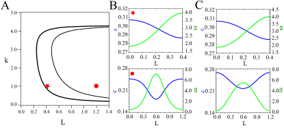
Figure 3: System behaviour in the deterministic limit. A) State diagram as a function of the dimensionless system length $L$ and the dimensionless detachment rate $k$. B) Steady states of the dynamic equations (17) and (18). C) Steady states of the reduced equations (54)-(59) where $C_{0}$, $C_{1}$, $C_{2}$, and $M_{0}$ have been adiabatically eliminated. Parameter values for $k$ and $L$ in (B) and (C) are indicated by the symbols in (A), $D=0.01$, and $C_{\mathrm{tot}}=\sqrt{10}$ .

Increasing the system length beyond $L_{\mathrm{c}}$, there is a second bifurcation at $L=L_{c,2}(k)$ through which two new solutions appear. They correspond to states, where the proteins either pile up in the cell center or accumulate at both poles. Numerical integration of the deterministic equations (17) and (18) indicates that only the state with proteins clustering in the center is stable, see Fig. 3B.

We can make a Galerkin ansatz and truncate the series (20) and (21) at a finite value of $n$. The dynamic equations resulting after insertion of the truncated series in Eqs. (17) and (18) are given in Appendix A. It turns out that for $L\lesssim L_{c,2}$ a series with $n=2$ gives a faithful description of the system dynamics, see Fig. 3C. Furthermore, the modes $C_{0}$, $C_{1}$, $C_{2}$, and $M_{0}$ relax on faster time scales than the modes $M_{1}$ and $M_{2}$, such that we can make an adiabatic approximation and express the former in terms of the latter. The dynamic equations thus only depend on $M_{1}$ and $M_{2}$.

In Figure 4, we present the flow field for the dynamic equations for $M_{1}$ and $M_{2}$ after adiabatic elimination of $C_{0}$, $C_{1}$, $C_{2}$, and $M_{0}$. For $L_{\mathrm{c}}\leq L\leq L_{c,2}$, the system has two symmetric stable and one hyperbolic fixed point, see Fig. 4A. The hyperbolic fixed point is at $(0,0,0,0)$ and corresponds to the homogenous state. The symmetric fixed points have $|M_{2}|\ll|M_{1}|$ such that they correspond to protein accumulations at either of the two poles. As soon as $L>L_{c,2}$ two new fixed points appear. These hyperbolic fixed points have $M_{1}=0$ and correspond to symmetric protein distribution with, respectively, accumulation in the center and simultaneous accumulation at both poles. Further increase of $L$ leads to two new hyperbolic fixed points. At the same time, the fixed point with $M_{1}<0$ becomes stable. It should be noted, though, that the corresponding symmetric distribution is not observed in the stochastic simulations, indicating that this fixed point remains hyperbolic if higher modes are taken into account. The two new hyperbolic fixed points are connected to the stable fixed points by heteroclinic orbits, see Fig. 4B.

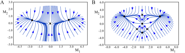
Figure 4: Flow field for the modes $M_{1}$ and $M_{2}$ in the deterministic limit for $L_{\mathrm{c}}\leq L\leq L_{c,2}$ (A) and $L_{c,2}\leq L$ (B). Black dots indicate stable and unstable fixed points, black crosses hyperbolic fixed points. Parameters are as in Fig. 3 and $L=0.52$ (A) and $L=1.2$ (B).

III.3 Galerkin approximation for the Fokker-Planck equation

We will now exploit the findings of the previous subsection and use the Galerkin approximation for the Fokker-Planck Equation (7). We will use the same dimensionless parameters and densities as above. Employing Equations (20) and (21), we can transform the functional $P[c(x),m(x);t]$ into a function of the coefficients $C_{n}$ and $M_{n}$, $n=0,1,2,\ldots$ The corresponding Fokker-Planck Equation can be derived from Eq. (7). To this end, we first express the functional derivatives with respect to $c(x)$ and $m(x)$ in terms of partial derivatives with respect to $C_{n}$ and $M_{n}$, $n=0,1,2,\ldots$ Considering a variation $\delta C_{n}$ of mode $n$ of membrane-bound molecules yields $\delta c(x)=\delta C_{n}\cos(n\pi x/L)$. If $\bar{F}$ denotes the function of $C_{n}$ and $M_{n}$ corresponding to a functional $F[c(x),m(x)]$, then

$$\frac{\partial\bar{F}}{\partial C_{n}} =\int_{0}^{L}dx\frac{\delta F}{\delta c(x)}\cos\left(\frac{n\pi x}{L}\right)$$ (29)

and analogously for the derivatives $\partial\bar{F}/\partial M_{n}$. Note, that variations of $C_{0}$ and $M_{0}$ are not independent as $C_{0}+M_{0}=1/L$. From the above expression follows that

$$\frac{\delta F}{\delta c(x)} =\frac{2}{L}\sum_{n=0}^{\infty}\frac{\partial\bar{F}}{\partial C_{n}}\cos\left(\frac{n\pi x}{L}\right)$$ (30)

$$\frac{\delta F}{\delta m(x)} =\frac{2}{L}\sum_{n=0}^{\infty}\frac{\partial\bar{F}}{\partial M_{n}}\cos\left(\frac{n\pi x}{L}\right)$$ (31)

and similarly

$$\frac{\delta^{2}F}{\delta c(x)\delta c(y)} =\frac{4}{L^{2}}\sum_{n,m=0}^{\infty}\frac{\partial^{2}\bar{F}}{\partial C_{n}\partial C_{m}}\cos\left(\frac{n\pi x}{L}\right)\cos\left(\frac{m\pi x}{L}\right)$$ (32)

$$\frac{\delta^{2}F}{\delta c(x)\delta m(y)} =\frac{4}{L^{2}}\sum_{n,m=0}^{\infty}\frac{\partial^{2}\bar{F}}{\partial C_{n}\partial M_{m}}\cos\left(\frac{n\pi x}{L}\right)\cos\left(\frac{m\pi x}{L}\right)$$ (33)

$$\frac{\delta^{2}F}{\delta m(x)\delta m(y)} =\frac{4}{L^{2}}\sum_{n,m=0}^{\infty}\frac{\partial^{2}\bar{F}}{\partial M_{n}\partial M_{m}}\cos\left(\frac{n\pi x}{L}\right)\cos\left(\frac{m\pi x}{L}\right).$$ (34)

Inserting the expansions (20) and (21) into Eq. (7), using the expressions for the functional derivatives just derived, and performing the integrals, we obtain a Fokker-Planck Equation for the probability density $P(\{C_{n}\}_{n=0,1,\ldots},\{M_{n}\}_{n=0,1,\ldots};t)$, where again $C_{0}+M_{0}=1/L$. It is of the form

$$\frac{\partial P}{\partial t}= -\sum_{n=0}^{\infty}\left\{\frac{\partial}{\partial C_{n}}\bar{A}_{\mathrm{c},n}+\frac{\partial}{\partial M_{n}}\bar{A}_{\mathrm{m},n}\right\}P$$ (35)

$$+\frac{1}{2\Omega}\sum_{n,m=0}^{\infty}\left\{\frac{\partial^{2}}{\partial C_{n}\partial C_{m}}\bar{B}_{\mathrm{cc},nm}+2\frac{\partial^{2}}{\partial C_{n}\partial M_{m}}\bar{B}_{\mathrm{cm},nm}+\frac{\partial^{2}}{\partial M_{n}\partial M_{m}}\bar{B}_{\mathrm{mm},nm}\right\}P.$$

We will now apply the Galerkin approximation and truncate the series at $n,m=2$. Furthermore, we will make the adiabatic approximation and express $C_{0}$, $C_{1}$, $C_{2}$, and $M_{0}$ in terms of $M_{1}$ and $M_{2}$ by using the deterministic equations (54)-(57) in steady state. Eventually, we arrive at

$$\partial_{t}P =-\partial_{k}u_{k}P+\frac{1}{2\Omega L^{\prime}}\partial_{k}\partial_{l}D_{kl}P,$$ (36)

where the probability distribution $P\equiv P(M_{1},M_{2};t)$ now depends only on $M_{1}$ and $M_{2}$ and where $\partial_{k}\equiv\partial/\partial M_{k}$ with $k=1,2$. Furthermore, $L^{\prime}=L\sqrt{D_{\mathrm{c}}/\omega_{\mathrm{c}}}$ and summation over repeating indices is understood. The expressions for the drift velocity $u_{k}=\dot{M}_{k}$ are those given above in the deterministic limit, Eqs. (58) and (59). The expressions for the diffusion matrix $\mathsf{D}$ are given in Appendix A. Note, that the elements $D_{kl}$ depend on $M_{1}$ and $M_{2}$.

In the next section, we will use the Fokker-Planck Equation (36) to determine the average switching time.

IV Estimation of the switching time in the weak noise limit

The switching time can equivalently be interpreted as the mean first-passage time (MFPT) of a multi-dimensional escape problem. However, in contrast to most cases studied in the literature, the deterministic dynamics is in the present case not determined by a potential, so that we cannot use Kramers (or Eyring) rate theory. Instead, we will employ a generalised framework developed by Maier and Stein Maier:1993vv . In a first step, we will present the necessary expressions and then compare their solution to data obtained from stochastic simulations. We continue to use the dimensionless parameters introduced above.

IV.1 Probability flux across the separatrix

As we had seen above, in the deterministic case there is a region in parameter space, where two stable mirror-symmetric distributions co-exist. The two basins of attraction are separated by a separatrix along $M_{1}=0$, which contains another fixed point, namely the homogenous state $M_{1}=M_{2}=0$. It is a hyperbolic fixed point for which the stable manifold coincides with the separatrix. The aim is now to calculate the MFPT $\tau$ in the limit of weak noise.

To this end, we consider the Fokker-Planck equation (36) with absorbing boundary conditions along the separatrix. We will calculate the total probability current across the separatrix associated with the eigenfunction $P_{1}$ of the Fokker-Planck operator that decays most slowly. Normalising this current to the total probability to find a particle on one side of the separatrix yields

$$\tau=\frac{-\int_{-\infty}^{\infty}\frac{1}{2\Omega L^{\prime}}\partial_{k}D_{1k}P(0,M_{2})dM_{2}}{\int_{0}^{\infty}\int_{-\infty}^{\infty}P(M_{1},M_{2})dM_{2}dM_{1}},$$ (37)

where summation with respect to the index $k$ is understood. Note, that $\tau$ is just the characteristic time on which the eigenfunction $P_{1}$ relaxes, that is, it is the inverse of the corresponding eigenvalue. In lowest order in $1/\Omega$, the eigenfunction $P_{1}$ can be replaced by the solution $P_{\mathrm{s}}$ to the steady-state Fokker-Planck Equation Naeh:1990up .

The steady state of Eq. (36) cannot be calculated exactly. Instead, we will make a Wentzel-Kramers-Brillouin ansatz and write the steady state probability distribution as

$$P_{\mathrm{s}}(M_{1},M_{2}) =K(M_{1},M_{2})\exp\{-\Omega L^{\prime}S(M_{1},M_{2})\}$$ (38)

with the classical action (or quasi-potential) $S$. The equation for the action is obtained by inserting the WKB ansatz into Eq. (36) and by considering the terms of first order in $1/\Omega$. We get an equation of the form of a Hamilton-Jacobi Equation $H(M_{1},M_{2},\partial_{1}S,\partial_{2}S)=0$ with the Hamiltonian

$$H =u_{k}p_{k}+\frac{1}{2}D_{kl}p_{k}p_{l},$$ (39)

where $p_{k}=\partial_{k}S$ is the momentum conjugated to $M_{k}$, $k=1,2$. The action is then obtained from solving first the canonical dynamic equations, which in our case read

$$\dot{M}_{k} =u_{k}+D_{kl}p_{l}$$ (40)

$$\dot{p}_{k} =-(\partial_{k}u_{l})p_{l}-\frac{1}{2}(\partial_{k}D_{lm})p_{l}p_{m},$$ (41)

and then the dynamic equation

$$\dot{S} =D_{kl}p_{k}p_{l}+u_{k}p_{k}.$$ (42)

It remains to determine the pre-factor $K$ in Eq. (38), which can be obtained from the terms of second order in $1/\Omega$ in Eq. (36). Explicitly,

$$\dot{K} =-\left[\partial_{k}(u_{k}+D_{kl}p_{l})+\frac{1}{2}W_{kl}D_{kl}\right]K.$$ (43)

In this expression $\mathsf{W}$ denotes the Hessian of the action $S$, that is, $W_{kl}=\partial_{k}\partial_{l}S$. It can be determined without knowledge of the action by solving its time evolution equation, which follows a (generalised) Riccati equation

$$\dot{W_{kl}}=-W_{km}D_{mn}W_{nl}-\left(\partial_{k}\dot{M}_{n}\right)W_{nl}-\left(\partial_{l}\dot{M}_{n}\right)W_{nk}+\frac{1}{2}\left(\partial_{l}\dot{p}_{k}+\partial_{k}\dot{p}_{l}\right).$$ (44)

In Figure 5, we present the steady state probability distribution corresponding to the phase portraits displayed on Fig. 4A. The probability is maximal in the vicinity of the stable fixed points. In the hyperbolic fixed point at $(0,0,0,0)$ the probability distribution has a saddle point (slight deviations are due to interpolation errors) and the heteroclinic orbit indicated in blue follows the ridge of probability distribution.

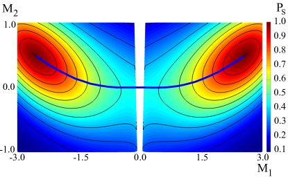
Figure 5: Steady state probability distribution in the WKB approximation. The blue curve indicates the heteroclinic orbit between the two stable fixed points passing through the hyperbolic fixed point at $(0,0,0,0)$. Parameters are as in Fig. 3 with $L=0.52$ and $\Omega=30$.

We can exploit the form of the probability distribution to further simplify Eq. (37). The integrand in the denominator of the above expression for $\tau$ is obviously dominated by the region around the stable fixed point, whereas the integrand in the numerator is dominated by the region around the hyperbolic fixed point $M_{1}=M_{2}=p_{1}=p_{2}=0$. In these regions, we can make a Gaussian approximation of the probability density or, equivalently, use a quadratic approximation of the Hamiltonian (39):

$$H =\lambda_{kl}M_{k}p_{l}+D_{kl}p_{k}p_{l},$$ (45)

where $\lambda_{kl}\equiv\partial_{k}u_{l}$ and where the coefficients are evaluated in the hyperbolic or stable fixed points of Eqs. (58) and (59), respectively. With this approximation, the switching time is estimated as

$$\tau =\frac{\pi}{\lambda^{\mathrm{hyp}}_{11}K^{\mathrm{hyp}}}\sqrt{\frac{|\mathrm{det}\ \mathsf{W}^{\mathrm{hyp}}|}{\mathrm{det}\ \mathsf{W}^{\mathrm{st}}}}\mathrm{exp}\{\Omega L^{\prime}S^{\mathrm{hyp}}\}.$$ (46)

In this expression, the quantities with a superscript ’hyp’ are evaluated in the hyperbolic fixed point, whereas a superscript ’st’ indicates evaluation in the stable fixed point.

Finally, the expression for $\det\mathsf{W}^{\mathrm{st}}$ and $\det\mathsf{W}^{\mathrm{hyp}}$ can be obtained from Eq. (44) by setting the time-derivative equal to zero and using $p_{1}=p_{2}=0$. It yields

$$W_{km}D_{mn}W_{nl}+\left(\partial_{l}u_{n}\right)W_{nk}+\left(\partial_{k}u_{n}\right)W_{nl}=0.$$ (47)

The elements $D_{mn}$ and the partial derivatives $\partial_{m}u_{n}$ again have to be evaluated at the respective fixed point.

We have now given all the elements necessary for estimating the switching time $\tau$.

IV.2 Comparison of the estimated switching time with stochastic simulations

According to Eq. (37), we need to evaluate various quantities in the fixed points of Eqs. (58) and (59). In the hyperbolic fixed point, the approximate Hamiltonian (45) can be obtained analytically. The matrices $\mathsf{\lambda}$ and $\mathsf{D}$ are diagonal with non-zero elements

$$\lambda^{\mathrm{hyp}}_{11} =\frac{\pi^{2}}{L^{2}}\left(\frac{2C_{0}M_{0}-k}{1+M_{0}^{2}+\frac{\pi^{2}}{L^{2}}}-D\right)$$ (48)

$$\lambda^{\mathrm{hyp}}_{22} =\frac{4\pi^{2}}{L^{2}}\left(\frac{2C_{0}M_{0}-k}{1+M_{0}^{2}+\frac{4\pi^{2}}{L^{2}}}-D\right)$$ (49)

$$D^{\mathrm{hyp}}_{11}=D^{\mathrm{hyp}}_{22} =4kM_{0}.$$ (50)

From this we get for the determinant of the Hessian

$$\det\mathsf{W}^{\mathrm{hyp}} =\frac{\lambda^{\mathrm{hyp}}_{11}\lambda^{\mathrm{hyp}}_{22}}{4k^{2}M_{0}^{2}}$$ (51)

The corresponding expressions for the stable fixed point have to be calculated numerically. The values of $K^{\mathrm{hyp}}$ and $S^{\mathrm{hyp}}$ in Eq. (46) require integration of the dynamic equations (40)-(43) along the heteroclinic orbit connecting the stable and the hyperbolic fixed points. Due to the non-linear character of the dynamic equations, these integrations also have to be performed numerically.

To determine the heteroclinic orbit, we used initial conditions such that $M_{1}$ and $M_{2}$ were located in the stable fixed point of Eqs. (58) and (59) and the energy was fixed to zero. These conditions left one of the generalised momenta $p_{1}$ and $p_{2}$ undetermined. Its value was obtained by minimising the distance of the corresponding trajectory to the hyperbolic fixed point at the origin.

In Figure 6, we present the results of our calculation for various cell lengths. The agreement between the simulation results and the approximate expression (37) for the switching time is remarkably good taking into account the various approximations we made along the way. The dependence of the switching time $\tau$ on the total molecule number $\Omega$ is exponential as indicated by Eq. (37). Its dependence on the cell length $L$ is also essentially exponential, suggesting that its dominant contribution of $L$ to $\tau$ is given by the explicit dependence on $L$ in Eq. (37). This result is in line with the observation made in Ref. FischerFriedrich:2010hv , that intracellular fluctuations decrease with increasing cell length.

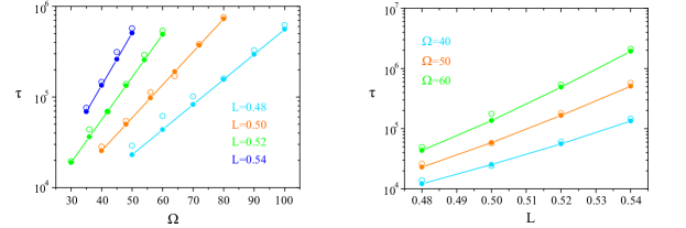
Figure 6: Comparison between the estimated switching time (full circles) and switching times measured in stochastic simulations (open circles) as a function of the total number of molecules $\Omega$ (A) and the dimensionless system length $L$ (B).

V Discussion

In this work, we have studied the influence of molecular noise on the self-organised polar localisation of proteins in rod-shaped bacteria. We found that cooperative attachment to the cell membrane is sufficient to generate asymmetric protein distributions along the bacterial long axis. Using stochastic simulations and an approximate analysis of the weak-noise limit we found that fluctuations in the protein distribution can lead to switches between two mirror-symmetric solutions. The frequency of these switches decreases exponentially with the cell length. This finding is in line with experimental observations on the Min-protein system in E. coli FischerFriedrich:2010hv . It suggests that the stability of spatial patterns in rod-shaped bacteria depends more on the total protein number in the cell than the protein density.

Here, we have restricted attention to the weak-noise limit, which is inherent to the use of a Fokker-Planck equation. It will be interesting to see in future work, whether the approach can be extended to stronger noise. For example, one might use the approach developed in Ref. Wu:2013dx to study the stability of the heterogenous states as a function of the total protein number and estimate the minimal number of molecules needed to achieve polar localisation.

The mechanism of self-organisation we have analysed, is based on cooperative binding of the molecules to a support and their spontaneous unbinding. Other molecular mechanisms might be considered. For example, we looked at the case that membrane-bound proteins exist in two states. Proteins bind in a cooperative manner in one state to the membrane and then transit into a second state in which they can unbind from the membrane. In a cellular context, the transition could be linked to the hydrolysis of ATP. If the transition between the two states occurs spontaneously, then the system behaviour is similar to the one discussed above. If proteins in the second state can induce detachment of proteins in the first state, then the switching time will decrease with increasing protein number and system length. This behaviour is similar to the one found for the Min proteins FischerFriedrich:2010hv ; Bonny:2013gt . Remarkably, if proteins in the second state only catalyse the transition of proteins in state one to state two, then the system can spontaneously oscillate. Additional cooperative effects thus can have a significant influence on the system behaviour.

A possible biological implication of our findings is that (self-organised) protein structures become less sensitive to molecular noise as a cell ages. Indeed, as the cell grows, the number of molecules as well as the stability of molecular assemblies at one of the cell poles increase. Similarly Min-protein oscillations in E. coli were observed to become less noisy with increasing cell length FischerFriedrich:2010hv . It will be interesting to see, whether the techniques used in the present work will allow us to gain a deeper understanding of this phenomenon, too.

Appendix A The dynamic equations in the Galerkin approximation

As indicated in the main text, we can stop the expansion in Eqs. (20) and (21) at $n=2$,

$$c(x,t) =C_{0}(t)+C_{1}(t)\cos(\pi x/L)+C_{2}(t)\cos(2\pi x/L)$$ (52)

$$m(x,t) =M_{0}(t)+M_{1}(t)\cos(\pi x/L)+M_{2}(t)\cos(2\pi x/L),$$ (53)

and still capture the essential features of the system dynamics. Inserting these expressions in Eqs. (17) and (18) and integrating with respect to $x$, we obtain

$$\dot{C}_{0} =-\left(1+M_{0}^{2}+\frac{1}{2}M_{1}^{2}+\frac{1}{2}M_{2}^{2}\right)C_{0}-\left(M_{0}M_{1}+\frac{1}{2}M_{1}M_{2}\right)C_{1}-\left(M_{0}M_{2}+\frac{1}{4}M_{1}^{2}\right)C_{2}+kM_{0}$$ (54)

$$\dot{C}_{1} =-\left(\frac{\pi}{L}\right)^{2}C_{1}-\left(2M_{0}M_{1}+M_{1}M_{2}\right)C_{0}-\left(1+M_{0}^{2}+M_{0}M_{2}+\frac{3}{4}M_{1}^{2}+\frac{1}{2}M_{2}^{2}\right)C_{1}-\left(M_{0}M_{1}+M_{1}M_{2}\right)C_{2}+kM_{1}$$ (55)

$$\dot{C}_{2} =-\left(\frac{2\pi}{L}\right)^{2}C_{2}-\left(2M_{0}M_{2}+\frac{1}{2}M_{1}^{2}\right)C_{0}-\left(M_{0}M_{1}+M_{1}M_{2}\right)C_{1}-\left(1+M_{0}^{2}+\frac{1}{2}M_{1}^{2}+\frac{3}{4}M_{2}^{2}\right)C_{2}+kM_{2}$$ (56)

$$\dot{M}_{0} =\left(1+M_{0}^{2}+\frac{1}{2}M_{1}^{2}+\frac{1}{2}M_{2}^{2}\right)C_{0}+\left(M_{0}M_{1}+\frac{1}{2}M_{1}M_{2}\right)C_{1}+\left(M_{0}M_{2}+\frac{1}{4}M_{1}^{2}\right)C_{2}-kM_{0}$$ (57)

$$\dot{M}_{1} =-D\left(\frac{\pi}{L}\right)^{2}M_{1}+\left(2M_{0}M_{1}+M_{1}M_{2}\right)C_{0}+\left(1+M_{0}^{2}+M_{0}M_{2}+\frac{3}{4}M_{1}^{2}+\frac{1}{2}M_{2}^{2}\right)C_{1}+\left(M_{0}M_{1}+M_{1}M_{2}\right)C_{2}-kM_{1}$$ (58)

$$\dot{M}_{2} =-D\left(\frac{2\pi}{L}\right)^{2}M_{2}+\left(2M_{0}M_{2}+\frac{1}{2}M_{1}^{2}\right)C_{0}+\left(M_{0}M_{1}+M_{1}M_{2}\right)C_{1}+\left(1+M_{0}^{2}+\frac{1}{2}M_{1}^{2}+\frac{3}{4}M_{2}^{2}\right)C_{2}-kM_{2}$$ (59)

The coefficients of the diffusion matrix $\mathsf{D}$ in Eq. (36) then read

$$D_{11}= \left(2+2M_{0}^{2}+\frac{3}{2}M_{1}^{2}+M_{2}^{2}+2M_{0}M_{2}\right)C_{0}+\left(3M_{0}M_{1}+2M_{1}M_{2}\right)C_{1}$$

$$+\left(1+M_{0}^{2}+M_{1}^{2}+\frac{3}{4}M_{2}^{2}+2M_{0}M_{2}\right)C_{2}+2kM_{0}+\left(k-4\frac{\pi^{2}}{L^{2}}D\right)M_{2}$$ (60)

$$D_{12}=D_{21}= \left(2M_{0}M_{1}+2M_{1}M_{2}\right)C_{0}+\left(1+M_{0}^{2}+M_{1}^{2}+\frac{3}{4}M_{2}^{2}+2M_{0}M_{2}\right)C_{1}$$

$$+\left(2M_{0}M_{1}+\frac{3}{2}M_{1}M_{2}\right)C_{2}+\left(k-4\frac{\pi^{2}}{L^{2}}D\right)M_{1}$$ (61)

$$D_{22}= \left(2+2M_{0}^{2}+M_{1}^{2}+\frac{3}{2}M_{2}^{2}\right)C_{0}+\left(2M_{0}M_{1}+\frac{3}{2}M_{1}M_{2}\right)C_{1}$$

$$+\left(\frac{3}{4}M_{1}^{2}+3M_{0}M_{2}\right)C_{2}+2kM_{0},$$ (62)

where $M_{0}$, $C_{0}$, $C_{1}$, and $C_{2}$ are expressed in terms of $M_{1}$ and $M_{2}$ by solving Eqs. (54)-(57) in steady state.

References

- (1) Shapiro L, McAdams HH, Losick R. Why and how bacteria localize proteins. Science (New York, NY). 2009 Nov;326(5957):1225–1228.
- (2) Kruse K. Bacterial Organization in Space and Time. In: Wirtz D, editor. E.H. Egelman, editor: Comprehensive Biophysics, Vol 7, Cell Biophysics. Academic Press, Oxford; 2012. p. 208–221.
- (3) Maddock JR, Shapiro L. Polar location of the chemoreceptor complex in the Escherichia coli cell. Science. 1993 Mar;259(5102):1717–1723.
- (4) Quisel JD, Lin DC, Grossman AD. Control of development by altered localization of a transcription factor in B. subtilis. Mol Cell. 1999 Nov;4(5):665–672.
- (5) Marston AL, Errington J. Dynamic movement of the ParA-like Soj protein of B. subtilis and its dual role in nucleoid organization and developmental regulation. Mol Cell. 1999 Nov;4(5):673–682.
- (6) Raskin DM, de Boer PAJ. Rapid pole-to-pole oscillation of a protein required for directing division to the middle of Escherichia coli. Proc Natl Acad Sci USA. 1999 Apr;96(9):4971–4976.
- (7) Bi EF, Lutkenhaus J. FtsZ ring structure associated with division in Escherichia coli. Nature. 1991 Nov;354(6349):161–164.
- (8) Bazylinski DA, Frankel RB. Magnetosome formation in prokaryotes. Nat Rev Microbiol. 2004 Mar;2(3):217–230.
- (9) Chevance FFV, Hughes KT. Coordinating assembly of a bacterial macromolecular machine. Nat Rev Microbiol. 2008 Jun;6(6):455–465.
- (10) Duke TA, Bray D. Heightened sensitivity of a lattice of membrane receptors. Proc Natl Acad Sci USA. 1999 Aug;96(18):10104–10108.
- (11) Loose M, Kruse K, Schwille P. Protein self-organization: lessons from the min system. Annu Rev Biophys. 2011 Jun;40:315–336.
- (12) Kerr RA, Levine H, Sejnowski TJ, Rappel WJ. Division accuracy in a stochastic model of Min oscillations in Escherichia coli. Proc Natl Acad Sci USA. 2006 Jan;103(2):347–352.
- (13) Fange D, Elf J. Noise-induced Min phenotypes in E. coli. PLoS Comput Biol. 2006 Jun;2(6):e80.
- (14) Arjunan SNV, Tomita M. A new multicompartmental reaction-diffusion modeling method links transient membrane attachment of E. coli MinE to E-ring formation. Syst Synth Biol. 2010 Mar;4(1):35–53.
- (15) Eldar A, Elowitz MB. Functional roles for noise in genetic circuits. Nature. 2010 Sep;467(7312):167–173.
- (16) Balázsi G, van Oudenaarden A, Collins JJ. Cellular Decision Making and Biological Noise: From Microbes to Mammals. Cell. 2011 Mar;144(6):910–925.
- (17) Doubrovinski K, Howard M. Stochastic model for Soj relocation dynamics in Bacillus subtilis. Proc Natl Acad Sci USA. 2005 Jul;102(28):9808–9813.
- (18) Fischer-Friedrich E, Meacci G, Lutkenhaus J, Chaté H, Kruse K. Intra- and intercellular fluctuations in Min-protein dynamics decrease with cell length. Proc Natl Acad Sci USA. 2010 Apr;107(14):6134–6139.
- (19) Sliusarenko O, Heinritz J, Emonet T, Jacobs-Wagner C. High-throughput, subpixel precision analysis of bacterial morphogenesis and intracellular spatio-temporal dynamics. Mol Microbiol. 2011 May;80(3):612–627.
- (20) Bonny M, Fischer-Friedrich E, Loose M, Schwille P, Kruse K. Membrane Binding of MinE Allows for a Comprehensive Description of Min-Protein Pattern Formation. PLoS Comput Biol. 2013 Dec;9(12):e1003347.
- (21) Howard M, Kruse K. Cellular organization by self-organization: mechanisms and models for Min protein dynamics. J Cell Biol. 2005 Feb;168(4):533–536.
- (22) Loose M, Fischer-Friedrich E, Ries J, Kruse K, Schwille P. Spatial regulators for bacterial cell division self-organize into surface waves in vitro. Science. 2008 May;320(5877):789–792.
- (23) Zieske K, Schwille P. Reconstitution of pole-to-pole oscillations of min proteins in microengineered polydimethylsiloxane compartments. Angew Chem Int Ed Engl. 2013 Jan;52(1):459–462.
- (24) Ben-Jacob E, Bergman DJ, Matkowsky BJ, Schuss Z. Lifetime of Oscillatory Steady-States. Physical Review A. 1982;26(5):2805–2816.
- (25) Kupferman R, Kaiser M, Schuss Z, Ben-Jacob E. WKB Study of Fluctuations and Activation in Nonequilibrium Dissipative Steady-States. Physical Review A. 1992;45(2):745–756.
- (26) Maier RS, Stein DL. Escape problem for irreversible systems. Phys Rev E. 1993;48(2):931.
- (27) Roma DM, O’Flanagan RA, Ruckenstein AE, Sengupta AM, Mukhopadhyay R. Optimal path to epigenetic switching. Physical review E, Statistical physics, plasmas, fluids, and related interdisciplinary topics. 2005 Jan;71(1).
- (28) Assaf M, Roberts E, Luthey-Schulten Z. Determining the Stability of Genetic Switches: Explicitly Accounting for mRNA Noise. Phys Rev Lett. 2011;106(24).
- (29) Guérin T, Prost J, Joanny JF. Motion Reversal of Molecular Motor Assemblies due to Weak Noise. Physical Review Letters. 2011 Feb;106(6):068101.
- (30) Guérin T, Prost J, Joanny JF. Bidirectional motion of motor assemblies and the weak-noise escape problem. Phys Rev E. 2011 Oct;84(4):041901.
- (31) Huang KC, Meir Y, Wingreen NS. Dynamic structures in Escherichia coli: Spontaneous formation of MinE rings and MinD polar zones. Proc Natl Acad Sci USA. 2003;100(22):12724–12728.
- (32) Hildebrand M, Mikhailov AS. Mesoscopic Modeling in the Kinetic Theory of Adsorbates. J Phys Chem. 1996 Jan;100(49):19089–19101.
- (33) Elf J, Ehrenberg M. Spontaneous separation of bi-stable biochemical systems into spatial domains of opposite phases. Syst Biol. 2004;1(2):230–236.
- (34) Naeh T, Klosek MM, Matkowsky BJ, Schuss Z. A Direct Approach to the Exit Problem. Siam Journal on Applied Mathematics. 1990 Apr;50(2):595–627.
- (35) Wu W, Wang J. Potential and flux field landscape theory. I. Global stability and dynamics of spatially dependent non-equilibrium systems. The Journal of chemical physics. 2013;139(12):121920.