BRST-Symmetry Breaking and Bose-Ghost Propagator
in Lattice Minimal Landau Gauge

Abstract

The Bose-ghost propagator has been proposed as a carrier of the confining force in Yang-Mills theories in minimal Landau gauge. We present the first numerical evaluation of this propagator, using lattice simulations for the SU(2) gauge group in the scaling region. Our data are well described by a simple fitting function, which is compatible with an infrared-enhanced Bose-ghost propagator. This function can also be related to a massive gluon propagator in combination with an infrared-free (Faddeev-Popov) ghost propagator. Since the Bose-ghost propagator can be written as the vacuum expectation value of a BRST-exact quantity and should therefore vanish in a BRST-invariant theory, our results provide the first numerical manifestation of BRST-symmetry breaking due to restriction of gauge-configuration space to the Gribov region.

The study of color confinement in Yang-Mills theories in minimal Landau gauge is an active area of research Greensite:2011zz . Let us recall that, in this case, the gauge condition is implemented (see for example Vandersickel:2012tz and references therein) by restricting the functional integral over gauge-field configurations to the so-called Gribov region $\Omega$. This restriction can be achieved by adding a nonlocal term $S_{\mathrm{h}}$, the horizon function, to the usual Landau gauge-fixed Yang-Mills action $S_{\mathrm{YM}}+S_{\mathrm{gf}}$. One thus obtains the Gribov-Zwanziger (GZ) action $S_{\mathrm{GZ}}=S_{\mathrm{YM}}+S_{\mathrm{gf}}+\gamma^{4}S_{\mathrm{h}}$. The massive parameter $\gamma$, known as the Gribov parameter, is dynamically determined (in a self-consistent way) through the so-called horizon condition.

In order to localize the GZ action Vandersickel:2012tz one introduces a pair of complex-conjugate bosonic fields $(\overline{\phi}^{ac}_{\mu},\phi^{ac}_{\mu})$ and a pair of Grassmann complex-conjugate fields $(\overline{\omega}^{ac}_{\mu},\omega^{ac}_{\mu})$. Then, the GZ action can be written as $S_{\mathrm{GZ}}=S_{\mathrm{YM}}+S_{\mathrm{gf}}+S_{\mathrm{aux}}+S_{\gamma}$, where

$$\!\!\!\!\!\!\!\!\!\!S_{\mathrm{aux}} = \int\mathrm{d}^{\rm 4}x\,\Bigl{[}\overline{\phi}_{\mu}^{ac}\,\partial_{\nu}\left(D_{\nu}^{ab}\phi^{bc}_{\mu}\right)-\overline{\omega}_{\mu}^{ac}\,\partial_{\nu}\left(D_{\nu}^{ab}\omega^{bc}_{\mu}\right)$$ (1)

$$\;\;\;\qquad\qquad-g_{0}\left(\partial_{\nu}\overline{\omega}_{\mu}^{ac}\right)f^{abd}\,D_{\nu}^{be}\eta^{e}\phi_{\mu}^{dc}\Bigr{]}$$

$$\!\!\!\!\!\!\!\!\!\!S_{\gamma} = \int\mathrm{d}^{\rm 4}x\,\Bigl{[}\gamma^{2}D^{ba}_{\nu}\Bigl{(}\phi_{\nu}^{ab}+\overline{\phi}_{\nu}^{ab}\Bigr{)}-4\left(N_{c}^{2}-1\right)\gamma^{4}\Bigr{]}\,.$$ (2)

Here, $a,\,b,\,c,\,d$ and $e$ are color indices in the adjoint representation of the SU($N_{c}$) gauge group, $\mu$ and $\nu$ are Lorentz indices. Also, $g_{0}$ is the bare coupling constant, (${\overline{\eta}}^{b}$, $\eta^{b}$) are the Faddeev-Popov (FP) ghost fields, $D^{ab}_{\nu}=\delta^{ab}\partial_{\nu}+g_{0}f^{acb}A_{\nu}^{c}$ is the covariant derivative, $f^{abd}$ are the structure constants of the gauge group and repeated indices are always implicitly summed over. At the classical level, the total derivatives $\partial_{\nu}(\phi_{\nu}^{aa}+\overline{\phi}_{\nu}^{aa})$ in the definition of $S_{\gamma}$ can be neglected Vandersickel:2012tz ; Zwanziger:2009je .

Under the nilpotent BRST variation $s$ Baulieu:1983tg , the four auxiliary fields form two BRST doublets, i.e. $s\,\phi^{ac}_{\mu}=\omega^{ac}_{\mu}$, $s\,\omega^{ac}_{\mu}=0$, $s\,\overline{\omega}^{ac}_{\mu}=\overline{\phi}^{ac}_{\mu}$ and $s\,\overline{\phi}^{ac}_{\mu}=0$, giving rise to a BRST quartet. At the same time, one can check that the localized GZ theory is not BRST-invariant. Indeed, while $s\,(S_{\mathrm{YM}}+S_{\mathrm{gf}}+S_{\mathrm{aux}})=0$, one finds that $s\,S_{\gamma}\propto\gamma^{2}\neq 0$. Since a nonzero value for the Gribov parameter $\gamma$ is related to the restriction of the functional integration to the Gribov region $\Omega$, it is clear that BRST-symmetry breaking is a direct consequence of this restriction, as investigated in several works (see e.g. Zwanziger:2009je ; brst ; Sorella:2009vt ; Zwanziger:2010iz and references therein).

In order to study numerically the effect of the BRST-breaking term $S_{\gamma}$, one can consider the expectation value of a BRST-exact quantity. One such possibility is the correlation function

$$Q^{abcd}_{\mu\nu}(x,y)\,=\,\braket{\,\omega^{ab}_{\mu}(x)\,\overline{\omega}^{cd}_{\nu}(y)\,+\,\phi^{ab}_{\mu}(x)\,\overline{\phi}^{cd}_{\nu}(y)\,}\,,$$ (3)

which can be written as $\braket{\,s(\,\phi^{ab}_{\mu}(x)\,\overline{\omega}^{cd}_{\nu}(y))\,}$. Of course, while the above expectation value should be zero for a BRST-invariant theory, it does not necessarily vanish if BRST symmetry is broken (see, for example, the discussion in Ref. Sorella:2009vt ). Indeed, at tree level (and in momentum space) one finds Vandersickel:2012tz ; Gracey:2010df

$$Q^{abcd}_{\mu\nu}(p,p^{\prime})\,=\,\frac{\left(2\pi\right)^{4}\delta^{(4)}\left(p+p^{\prime}\right)\,g_{0}^{2}\,\gamma^{4}f^{abe}f^{cde}P_{\mu\nu}(p)}{p^{2}\,\left(p^{4}+2g_{0}^{2}N_{c}\gamma^{4}\right)}\,,$$ (4)

where $P_{\mu\nu}(p)$ is the usual transverse projector. Thus, this propagator is proportional to the Gribov parameter $\gamma$, i.e. its nonzero value is clearly related to the breaking of the BRST symmetry in the GZ theory.

On the lattice one does not have direct access to the auxiliary fields $(\overline{\phi}^{ac}_{\mu},\phi^{ac}_{\mu})$ and $(\overline{\omega}^{ac}_{\mu},\omega^{ac}_{\mu})$. On the other hand, by 1) adding suitable sources to the GZ action, 2) explicitly integrating over the four auxiliary fields —which enter the action at most quadratically— and 3) taking the usual functional derivatives with respect to the sources, one can verify that Zwanziger:2009je

$$\!\!\!\!\!\!\!\!Q^{abcd}_{\mu\nu}(x-y)\,=\,\gamma^{4}\,\left\langle\,R^{ab}_{\mu}(x)\,R^{cd}_{\nu}(y)\,\right\rangle\,,$$ (5)

where

$$R^{ac}_{\mu}(x)=\int\mathrm{d}^{\rm 4}z\,({\cal M}^{-1})^{ae}(x,z)\,B^{ec}_{\mu}(z)$$ (6)

and $B^{bc}_{\nu}(x)=g_{0}\,f^{bec}\,A^{e}_{\nu}(x)$. We remark that the notations used in Refs. Vandersickel:2012tz and Zwanziger:2009je are slightly different. Also, our $Q^{abcd}_{\mu\nu}(x,y)$ propagator corresponds to the $F$-term of the $V$-propagator in equations (72) and (75) of Ref. Zwanziger:2009je . Thus, the behavior of this propagator depends only on the bosonic fields $(\overline{\phi}^{ac}_{\mu},\phi^{ac}_{\mu})$. Finally, one should recall that this Bose-ghost propagator has been proposed as a carrier of long-range confining force in minimal Landau gauge Zwanziger:2009je ; Furui:2009nj ; Zwanziger:2010iz .

We evaluate the Bose-ghost propagator as defined in Eq. (5) above —modulo the global factor $\gamma^{4}$— using numerical simulations in the SU(2) case. In order to check discretization effects, we considered three different values of the lattice coupling $\beta$, i.e. $\beta=2.2$, $2.34940204$ and $2.43668228$, respectively corresponding Bloch:2003sk to a lattice spacing $a$ of about $0.210\,fm$, $0.140\,fm$ and $0.105\,fm$. For $\beta=2.2$ and $2.34940204$ we used five different lattice volumes, i.e. $V=16^{4}$, $24^{4}$, $32^{4}$, $40^{4}$, $48^{4}$ in the former case and $V=24^{4}$, $36^{4}$, $48^{4}$, $60^{4}$, $72^{4}$ in the latter case. These two sets yield (approximately) the same set of physical volumes, ranging from about $(3.366\,fm)^{4}$ to $(10.097\,fm)^{4}$. For $\beta=2.43668228$ we considered only the lattice volume $V=96^{4}$, which also corresponds to a physical volume of about $(10.097\,fm)^{4}$. Thermalized configurations have been gauge-fixed to lattice minimal Landau gauge using the stochastic-overrelaxation algorithm Cucchieri:1995pn , with a stopping criterion $(\partial_{\mu}\vec{A}_{\mu})^{2}\leq 10^{-14}$ (after averaging over the lattice volume and the three color components).

In order to evaluate the Bose-ghost propagator, we invert the FP matrix ${\cal M}^{ab}(x,y)$ for the sources $B^{bc}_{\mu}(x)$, after removing their zero modes. As for the lattice gauge field $A_{\mu}(x)$, corresponding to $ag_{0}A_{\mu}(x)$ in the continuum, we employ the usual unimproved definition $[U_{\mu}(x)-U^{\dagger}_{\mu}(x)]/(2i)$, where $U_{\mu}(x)$ are the lattice link variables entering the Wilson action. The inversion of the FP matrix is performed using a conjugate-gradient method, accelerated by even/odd preconditioning. If we indicate with $\widetilde{R}^{ac}_{\mu}(k)=V^{-1/2}\sum_{x}R^{ac}_{\mu}(x)\,\exp{(2\pi ik\cdot x/N)}$ the Fourier transform of the outcome $R^{ac}_{\mu}(x)$ of the numerical inversion [see Eq. (6)], then it is clear that we can evaluate the Bose-ghost propagator [see Eq. (5)] in momentum space by considering $\,Q^{abcd}_{\mu\nu}(k)\equiv\Re\{\,\widetilde{R}^{ab}_{\mu}(k)\widetilde{R}^{cd}_{\nu}(-k)\,\}$. In the above equations, $N$ is the lattice side, $k$ is the wave vector with components $k_{\mu}=0,1,\ldots,N-1$ and $\Re$ indicates the real part of the expression within brackets. Then, by contracting the $b$ and $d$ indices, we can write [see Eq. (4)]

$$Q^{ac}(k)\,\equiv\,Q^{abcb}_{\mu\mu}(k)\,\equiv\,\delta^{ac}N_{c}\,P_{\mu\mu}(k)\,Q(k^{2})\,,$$ (7)

due to global color invariance.

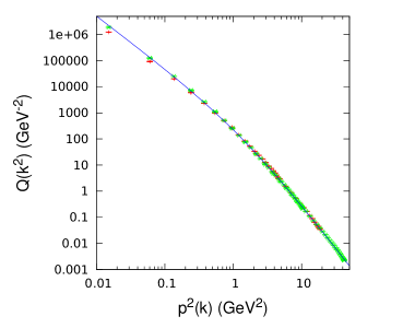
Figure 1: The Bose-ghost propagator $Q(k^{2})$, defined in Eq. (7), as a function of the improved momentum squared $p^{2}(k)$. We plot data for $\beta=2.2$, $V=48^{4}$ (red, $+$, 500 configurations) and $\beta=2.34940204$, $V=72^{4}$ (green, $\times$, 250 configurations), after applying a matching procedure matching . We also plot, for $V=72^{4}$, a fit using Eq. (8) and the parameters in Table 1, with $c=114(13)$. Note the logarithmic scale on both axes.

Numerical results for the scalar function $Q(k^{2})$, defined in the above equation, are shown in Figs. 1 and 2. In all cases the data points represent averages over gauge configurations and error bars correspond to one standard deviation. (We consider the statistical error only; the number of configurations ranges from 10000, for $V=16^{4}$ at $\beta=2.2$, to 100, for $V=96^{4}$ at $\beta=2.43668228$.) In the plots, all quantities are in physical units and we use the improved definition for the momenta, i.e. $p^{2}(k)=\sum_{\mu}(p_{\mu}^{2}+p_{\mu}^{4}/12)$ with $p_{\mu}=2\sin{(\pi k_{\mu}/N)}$, which makes the behavior of the propagator smoother, allowing a better fit to the data. In our simulations we considered two types of momenta, i.e. wave vectors whose components are $(0,0,0,k)$ and $(k,k,k,k)$, with $k=1,2,\ldots,N/2-1$. This gives $N-2$ different values for the momentum $p$. [Note that the null momentum trivially gives a zero result for the scalar function $Q(k^{2})$, since $\widetilde{R}^{ac}_{\mu}(0)=0$.] We also checked that the extrapolation to the infinite-volume limit is relevant only to clarify the infrared (IR) behavior of the propagator, i.e. finite-size effects —at a given lattice momentum $p$— are essentially negligible. Here, we did not check for possible Gribov-copy effects.

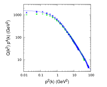
Figure 2: The product $Q(k^{2})p^{4}(k)$, as a function of the improved momentum squared $p^{2}(k)$. We plot data for $\beta=2.34940204$, $V=72^{4}$ (green, $\times$, 250 configurations) and $\beta=2.43668228$, $V=96^{4}$ (blue, $*$, 100 configurations), after applying a matching procedure matching to the former set of data. We also plot, for $V=96^{4}$, a fit using Eq. (8) and the parameters in Table 1, with $c=247(16)$. Note the logarithmic scale on both axes.

In Fig. 1 we show the data at $\beta=2.2$ with $V=48^{4}$ and at $\beta=2.34940204$ with $V=72^{4}$, after rescaling the data at $\beta=2.2$ using the matching technique described in Ref. matching . The data scale quite well, even though small deviations are observable in the IR limit (see also Fig. 2). We also fit the data using the fitting function

$$f(p^{2})\,=\,\frac{c}{p^{4}}\,\frac{p^{2}+s}{p^{4}\,+\,u^{2}p^{2}\,+\,t^{2}}\,.$$ (8)

Following the analysis in Zwanziger:2009je ; Zwanziger:2010iz , i.e. by using the relation (obtained using a cluster decomposition)

$$Q(p^{2})\,\sim\,g_{0}^{2}\,G^{2}(p^{2})\,D(p^{2})\,,$$ (9)

where $D(p^{2})$ is the gluon propagator and $G(p^{2})$ is the ghost propagator, the above fitting function corresponds to considering an infrared-free ghost propagator $G(p^{2})$ and a massive gluon propagator $D(p^{2})$ massive . The fit describes the data quite well (see the $\chi^{2}/\mbox{dof}$ values in Table 1). Let us note that the fitting value for the parameter $c$ is somewhat arbitrary, since one can always fix a renormalization condition foot1 at a given scale $p^{2}=\mu^{2}$, which in turn yields a rescaling of the Bose-ghost propagator by a global factor.

$V=N^{4}$	$\beta$	$t\,(GeV^{2})$	$u\,(GeV)$	$s\,(GeV^{2})$	$\chi^{2}/\mbox{dof}$
$\,48^{4}\,$	2.2	2.2(0.2)	1.5(0.2)	9.9(3.1)	6.28
$\,72^{4}\,$	2.34940204	3.2(0.3)	3.6(0.4)	46(13)	2.40
$\,96^{4}\,$	2.43668228	3.0(0.2)	3.9(0.3)	58.0(9.8)	1.12

Table 1: Parameters $t$, $u$ and $s$ from a fit of $f(x)$ in (8) to the data. Errors in parentheses correspond to one standard deviation. The number of degrees of freedom (dof) is always $N-6$. We also show the reduced chi-squared $\chi^{2}/\mbox{dof}$. Fits have been done using gnuplot.

On the other hand, the parameters $t$, $u$ and $s$ can be related to the analytic structure of the Bose-ghost propagator $Q(p^{2})$. For example, as done in Ref. Cucchieri:2011ig for the gluon propagator, one could try to rewrite the fitting function in terms of a pair of complex-conjugate poles. Then, we find that these poles are actually real and given by $7.6(1.2)\pm 7.0(1.3)$, where we used the data reported in the last line of Table 1. (Errors, shown in parentheses, correspond to one standard deviation and were obtained using propagation of error.) Thus, this fit supports the so-called massive solution of the coupled Yang-Mills Dyson-Schwinger equations of gluon and ghost propagators (see e.g. Ref. Aguilar:2008xm ) and the so-called Refined GZ approach RGZ . However, the values for the fitting parameters do not seem to relate in a simple way to the corresponding values obtained by fitting gluon-propagator data Cucchieri:2011ig .

Even though the simple Ansatz above gives a good description of the data, deviations can be seen in the IR region for momenta below about $1\,GeV$, by plotting the quantity $Q(k^{2})\,p^{4}(k)$ (see Fig. 2). We checked that one can slightly improve our fits, by using more general forms of the propagator. However, in these cases, most of the fitting parameters are determined with very large errors, suggesting that such fitting functions have too many (redundant) parameters. For this reason we do not show these fits here. (A more detailed analysis of the lattice data will be presented elsewhere.)

The above results allow a simple qualitative description of the momentum-space behavior of the Bose-ghost propagator. In particular, we find that its IR behavior is strongly enhanced, given by $p^{-4}$. This result is in agreement with the one-loop analysis carried out in Gracey:2009mj but not with the prediction of Ref. Zwanziger:2009je , where an IR-enhancement of $p^{-6}$ was obtained by considering in Eq. (9) an IR-enhanced ghost propagator and an IR-vanishing gluon propagator (see for example Refs. scaling ). One should stress that, even though a double-pole singularity is suggestive of a long-range interaction, the above result does not imply a linearly-rising potential between quarks. Indeed, when coupled to quarks via the $A-\phi$ propagator —which is nonzero due to the vertex term $\overline{\phi}_{\mu}^{ac}\,gf^{acb}A_{\nu}^{c}\partial_{\nu}\,\phi^{bc}_{\mu}$—, the Bose-ghost propagator gets a momentum factor at each vertex Zwanziger:2009je ; Zwanziger:2010iz , i.e. the effective propagator is given by $p^{-2}$ in the IR limit. This analysis is confirmed by the explicit evaluation of the static potential in Ref. Gracey:2009mj , considering a two-loop topology with the exchange of a Bose-ghost quantum. These results seem to suggest that a linearly rising potential cannot be obtained by a perturbative calculation based on a simple one-particle exchange, but requires a fully non-perturbative analysis. (For a lengthier discussion about this issue, the reader can refer, for example, to the last section in Ref. Gracey:2009mj .)

We conclude by stressing that, even though we did not explicitly evaluate the Gribov parameter $\gamma$ foot2 , our results constitute the first numerical manifestation of BRST-symmetry breaking due to the restriction of the functional integration to the Gribov region $\Omega$ in the GZ approach. This directly affects continuum functional approaches in Landau gauge (see for example bse and references therein), which usually employ lattice results in minimal Landau gauge as an input and/or as a comparison. At the same time, as stressed in Section 8 of the recent QCD review Brambilla:2014aaa , several questions are still open for a clear understanding, at the nonperturbative level, of the GZ approach. In particular, one should understand how a physical positive-definite Hilbert space could be defined in this case.

Acknowledgments: The authors thank S.P. Sorella for useful discussions. A. Cucchieri and T. Mendes acknowledge partial support from FAPESP (grant # 2009/50180-0) and from CNPq. D. Dudal and N. Vandersickel are supported by the Research Foundation-Flanders. We also would like to acknowledge computing time provided on the Blue Gene/P supercomputer supported by the Research Computing Support Group (Rice University) and Laboratório de Computação Científica Avançada (Universidade de São Paulo).

References

- (1) J. Greensite, Lect. Notes Phys. 821, 1 (2011).
- (2) N. Vandersickel and D. Zwanziger, Phys. Rept. 520, 175 (2012).
- (3) D. Zwanziger, arXiv:0904.2380 [hep-th].
- (4) L. Baulieu, Phys. Rept. 129, 1 (1985).
- (5) D. Zwanziger, Nucl. Phys. B412, 657 (1994); L. von Smekal, M. Ghiotti and A. G. Williams, Phys. Rev. D78, 085016 (2008); L. Baulieu and S. P. Sorella, Phys. Lett. B671, 481 (2009); D. Dudal and N. Vandersickel, Phys. Lett. B700, 369 (2011); P. Lavrov, O. Lechtenfeld and A. Reshetnyak, JHEP 1110, 043 (2011); A. Weber, J. Phys. Conf. Ser. 378, 012042 (2012); A. Maas, Mod. Phys. Lett. A27, 1250222 (2012); D. Dudal and S. P. Sorella, Phys. Rev. D86, 045005 (2012); M. A. L. Capri et al., Annals Phys. 339, 344 (2013); A. Reshetnyak, arXiv:1312.2092 [hep-th].
- (6) S. P. Sorella, Phys. Rev. D80, 025013 (2009).
- (7) D. Zwanziger, Phys. Rev. D81, 125027 (2010).
- (8) J. A. Gracey, Eur. Phys. J. C70, 451 (2010).
- (9) S. Furui, PoS LAT 2009, 227 (2009).
- (10) J. C. R. Bloch, A. Cucchieri, K. Langfeld and T. Mendes, Nucl. Phys. B687, 76 (2004).
- (11) A. Cucchieri and T. Mendes, Nucl. Phys. B471, 263 (1996).
- (12) D. B. Leinweber et al. [UKQCD Collaboration], Phys. Rev. D60, 094507 (1999) [Erratum-ibid. D61, 079901 (2000)]; A. Cucchieri, T. Mendes and A. R. Taurines, Phys. Rev. D67, 091502 (2003).
- (13) A. Cucchieri and T. Mendes, Phys. Rev. Lett. 100, 241601 (2008); Phys. Rev. D78, 094503 (2008); P. Boucaud et al., Few Body Syst. 53, 387 (2012).
- (14) From Eqs. (5) and (6) it is clear that the propagator evaluated in this work has a renormalization constant equal to one in the so-called algebraic renormalization scheme Vandersickel:2012tz . This implies that is also finite in any renormalization scheme.
- (15) A. Cucchieri, D. Dudal, T. Mendes and N. Vandersickel, Phys. Rev. D85, 094513 (2012).
- (16) A. C. Aguilar, D. Binosi and J. Papavassiliou, Phys. Rev. D78, 025010 (2008).
- (17) D. Dudal, J. A. Gracey, S. P. Sorella, N. Vandersickel and H. Verschelde, Phys. Rev. D78, 065047 (2008); D. Dudal, S. P. Sorella and N. Vandersickel, Phys. Rev. D84, 065039 (2011).
- (18) J. A. Gracey, JHEP 1002, 009 (2010).
- (19) D. Zwanziger, Phys. Rev. D65, 094039 (2002); C. S. Fischer and R. Alkofer, Phys. Lett. B536, 177 (2002); M. Q. Huber, R. Alkofer, C. S. Fischer and K. Schwenzer, Phys. Lett. B659, 434 (2008).
- (20) One should recall that the parameter is not explicitly introduced on the lattice, since the restriction of the gauge-configuration space to the region is achieved by numerical minimization. Thus, quantities proportional to , such as the Bose-ghost propagator considered here or the horizon function (see, e.g., Cucchieri:1997ns ), are always evaluated modulo the global factor.
- (21) A. Cucchieri, Nucl. Phys. B521, 365 (1998).
- (22) R. Alkofer and L. von Smekal, Phys. Rept. 353, 281 (2001); A. Bashir et al;, Commun. Theor. Phys. 58, 79 (2012).
- (23) N. Brambilla et al., arXiv:1404.3723 [hep-ph].